Most of theelectrical generators are powered by turbines. Turbines are the primemovers of
civilisation. Steam and Gas turbines share in the electrical power generation is about 75%.
About 20% of power is generated by hydraulic turbines and hence thier importance. Rest of 5%
only is by other means of generation. Hydraulic power depends on renewable source and hence
is ever lasting. It is also non polluting in terms of non generation of carbon dioxide.
The main components of hydraulic power plant are (i) The storage system. (ii) Conveying
system (iii) Hydraulic turbine with control system and (iv) Electrical generator
The storage system consists of a reservoir with a dam structure and the water flow
control in terms of sluices and gates etc. The reservoir may be at a high level in the case of
availability of such a location. In such cases the potential energy in the water will be large but
the quantity of water available will be small. The conveying system may consist of tunnels,
channels and steel pipes called penstocks. Tunnels and channels are used for surface conveyance.
Penstocks are pressure pipes conveying the water from a higher level to a lower level under
pressure. The penstock pipes end at the flow control system and are connected to nozzles at
the end. The nozzles convert the potential energy to kinetic energy in free water jets. These
jets by dynamic action turn the turbine wheels. In some cases the nozzles may be replaced by
guide vanes which partially convert potential energy to kinetic energy and then direct the
stream to the turbine wheel, where the remaining expansion takes place, causing a reaction
on the turbine runner. Dams in river beds provide larger quantities of water but with a lower
potential energy.
The reader is referred to books on power plants for details of the components and types
of plants and their relative merits. In this chapter we shall concentrate on the details and
operation of hydraulic turbines.
7.0 INTRODUCTION
7.1 HYDRAULIC POWER PLANT
Chapter-7 Hydraulic Turbines
186
2.
P-2D:N-fluidFlu14-1.pm5
The main classificationdepends upon the type of action of the water on the turbine. These are
(i) Impulse turbine (ii) Reaction Turbine. In the case of impulse turbine all the
potential energy is converted to kinetic energy in the nozzles. The imulse provided by the jets
is used to turn the turbine wheel. The pressure inside the turbine is atmospheric. This type is
found suitable when the available potential energy is high and the flow available is
comparatively low. Some people call this type as tangential flow units. Later discussion will
show under what conditions this type is chosen for operation.
(ii) In reaction turbines the available potential energy is progressively converted in the
turbines rotors and the reaction of the accelerating water causes the turning of the wheel.
These are again divided into radial flow, mixed flow and axial flow machines. Radial flow
machines are found suitable for moderate levels of potential energy and medium quantities of
flow. The axial machines are suitable for low levels of potential energy and large flow rates.
The potential energy available is generally denoted as “head available”. With this terminology
plants are designated as “high head”, “medium head” and “low head” plants.
Hydraulic turbines are mainly used for power generation and because of this these are large
and heavy. The operating conditions in terms of available head and load fluctuation vary
considerably. In spite of sophisticated design methodology, it is found the designs have to be
validated by actual testing. In addition to the operation at the design conditions, the
characteristics of operation under varying in put output conditions should be established. It is
found almost impossible to test a full size unit under laboratory conditions. In case of variation
of the operation from design conditions, large units cannot be modified or scrapped easily. The
idea of similitude and model testing comes to the aid of the manufacturer.
In the case of these machines more than three variables affect the characteristics of the
machine, (speed, flow rate, power, head available etc.). It is rather difficult to test each
parameter’s influence separately. It is also not easy to vary some of the parameters. Dimensional
analysis comes to our aid, for solving this problem. In chapter 8 the important dimension less
parameters in the case of turbomachines have been derived (problem 8.16).
The relevant parameters in the case of hydraulic machines have been identified in that
chapter. These are
1. The head coefficient, gH/N2D2
3
N3D5
1/2(gH)5/4
Consistant sets of units should be used to obtain numerical values. All the four
dimensionless numbers are used in model testing. The last parameter has particular value
when it comes to choosing a particular type under given available inputs and outputs. It has
been established partly by experimentation and partly by analysis that the specific speed to
some extent indicates the possible type of machine to provide the maximum efficiency under
the given conditions. Figure 14.1 illustrates this idea. The representation is qualitative only.
Note that as head decreases for the same power and speed, the specific speed increases.
7.2 CLASSIFICATION OF TURBINES
7.3 SIMILITUDE AND MODEL TESTING
(7.3.1)
2. The flow coefficient, Q/ND (7.3.2)
3. The power coefficient, P/ρ (7.3.3)
4. The specific sheed, N p/ρ
187
3.
P-2D:N-fluidFlu14-1.pm5
Pelton wheel
Francis turbines
Axialflow turbines
0.98
0.94
0.90
0.86
0.82
Efficiency,
h
100
90
80
70
60
50
40
2500
5000
10000
20000
30000
50000
80000
Efficiency
%
Specific speed
Over 50000
15000 to 50000
5000 to 15000
2
000
to
5000
1
0
00
to
2000
5
0
0
t
o
1000
Below
500
/min
l
Axial
Wider radial cshortor
Very narrow radial
0 1 2 3 4
Dimensionless specific speed (radian)
Figure 7.3.1 Variation of efficiency with specific speed.
Figure 7.3.2 gives another information provided by the specific speed. As flow rate
increases for the same specific speed efficiency is found also to increase. For the same flow
rate, there is an increase in efficiency with specific speed.
Figure 7.3.2 Variation of efficiency and flow passage with specific speed.
188
4.
P-2D:N-fluidFlu14-1.pm5
The type offlow passage also varies with specific speed as shown in the figure.
As the flow rate increases, the best shape is chosen for the maximum efficiency at that
flow. The specific speed is obtained from the data available at the location where the plant is
to be installed. Flow rate is estimated from hydrological data. Head is estimated from the
topography.
Power is estimated by the product of head and flow rate. The speed is specified by the
frequency of AC supply and the size. Lower the speed chosen, larger will be the size of the
machine for the same power. These data lead to the calculation of the specific speed for the
plant. The value of the specific speed gives a guidance about the choice of the type of machine.
Worked examples will illustrate the idea more clearly.
Ns =
N p
H5 4
/
where N is in rps, P in W and H in m. This is also shown in Table 14.1.
Table 14.1 provides some guidance about the type of turbine suitable at various ranges
of specific speeds.
Dimensionles Dimensional Type of turbine having the
specific specific speed best efficiency at these values
speed range in SI system
0.015—0.053 8—29 Single jet Pelton turbine
0.047—0.072 26—40 Twin jet Pelton turbine
0.72—0.122 40—67 Multiple jet Pelton turbine
0.122—0.819 67—450 Radial flow turbine Francis type (H < 350m)
0.663—1.66 364—910 Axial flow Kaplan turbine. (H < 60m)
There is considerable variation in the specific speeds indicated by various authors. Speed
N is used as rpm and power in kW by some authors.
Consider the following
N p
gH
ρ1/2 5 4
( ) /
→
1 1/2 1/2
1/2
3 2
1/2
10 4
5 4
S
N m
S
m
kg
s
m
. .
/ /
/
. m5/4
Substituting for Newton N1/2 as kg1/2 m1/2/s the expression will be dimensionless. This
can be checked
NS →
1 1/2 1/2 1/2
1/2
1 5
1/2
s
kg m m
s h
m
kg
s
m
s
. . .
. 2.5
2.5
→ M° L° T°
1 1/2
1
1/2 1/2
1/2
1 5 2 5
1/2 2 5
s
k m
s
m
s
m s
kg m
. . .
.
. .
. → M°L°T°
The expressions given in the equation 7.3.1 to 4 are dimensionless and will give the
same numerical value irrespective of the system of units adopted. In practice dimensional
specific speed is popularly used
Table Best specific Speed Range for Different Type of Hydraulic Turbines
Such use is dimensionly complex and will vary with values given in table 7.1. In the
non dimensional form, speed should be in rps and power should be in W. Then only the value
becomes dimensionless.
189
5.
P-2D:N-fluidFlu14-1.pm5
As a checkfor the dimensional value listed, the omitted quantities in this case are ρ1/2
g1.2
But in the solved problems and examples, these conditions are generally not satisfied. Even
with same actual installation data, the specific speed is found to vary from the listed best
values for the type.
Power estimated 40000 kW, Speed required : 417.5 rpm. Also indicate the suitable type of turbine
Dimensionless specific speed : units to be used :
N → rps, P → W or Nm/s, ρ → kg/m3, g →
m
s2 , H → m
∴ Ns =
417 5
60
40 000000
1000 9 81 900
1/2
1/2 5 4 5 4
. ( , )
. / /
×
× ×
= 0.0163.
Hence single jet pelton turbine is suitable.
Non dimensional specific speed.
Ns =
417 5
60
40 000000
900
1/2
5 4
. ,
/
× = 8.92.
50,000 kW. The sheed chosen is 600 rpm. Determine the specific speed. Indicate what type of
turbine is suitable.
= 549
∴ 0.015 × 549 = 8.24 as in the tabulation.
In the discussions the specific speed values in best efficiency is as given in table 7.1.
Example 1. Determine the specific speed for the data available at a location as given below
(Both dimensionless and dimensional). Head available : 900 m.
Significance of specific speed. Specific speed does not indicate the speed of the
machine. It can be considered to indicate the flow area and shape of the runner. When the
head is large, the velocity when potential energy is converted to kinetic energy will be high.
The flow area required will be just the nozzle diameter. This cannot be arranged in a fully
flowing type of turbine. Hence the best suited will be the impulse turbine. When the flow
increases, still the area required will be unsuitable for a reaction turbine. So multi jet unit is
chosen in such a case. As the head reduces and flow increases purely radial flow reaction
turbines of smaller diameter can be chosen. As the head decreases still further and the flow
increases, wider rotors with mixed flow are found suitable. The diameter can be reduced further
and the speed increased up to the limit set by mechanical design. As the head drops further for
the same power, the flow rate has to be higher. Hence axial flow units are found suitable in
this situation. Keeping the power constant, the specific speed increases with N and decreases
with head. The speed variation is not as high as the head variation. Hence specific speed value
increases with the drop in available head. This can be easily seen from the values listed in
table 7.1.
Agrees with the former value.
Single jet impulse turbine will be suitable.
Example.2 At a location the head available was estimated as 200 m. The power potential was
190
6.
P-2D:N-fluidFlu14-1.pm5
Dimensionless. N →rps, P → W, g →
m
kg
3
, g →
m
s2 , H → m
Ns =
600 40 000000
60 200 9 81 1000
5 4 1/2
,
( . ) /
× × ×
= 0.153.
Hence Francis type of turbine is suitable.
Dimensional. Ns =
600
60
40 000000
200
1/2
5 4
×
( , )
/ = 84.09.
Hence agrees with the previous value.
Dimensionless Ns =
600
60
40 000 000
1000 9 81 50
1/2 5 4
.
, ,
( . ) /
×
= 0.866
Hence axial flow Kaplan turbine is suitable.
Dimensional Ns =
600
60
40 000 000
50
1/2
1 25
×
, ,
. = 475.
It is found not desirable to rely completely on design calculations before manufacturing
a large turbine unit. It is necessary to obtain test results which will indicate the performance
of the large unit. This is done by testing a “homologous” or similar model of smaller size and
predicting from the results the performance of large unit. Similarity conditions are three fold
namely geometric similarity, kinematic similarity and dynamic similarity. Equal ratios of
geometric dimensions leads to geometric similarity.
Similar flow pattern leads to kinematic similarity. Similar dynamic conditions in terms
of velocity, acceleration, forces etc. leads to dynamic similarity. A model satisfying these
conditions is called “Homologous” model. In such case, it can be shown that specific speeds,
head coefficients flow coefficient and power coefficient will be identical between the model and
the large machine called prototype. It is also possible from these experiments to predict
part load performance and operation at different head speed and flow conditions.
The ratio between linear dimensions is called scale. For example an one eight
scale model means that the linear dimensions of the model is 1/8 of the linear dimensions of
the larger machine or the prototype. For kinematic and dynamic similarity the flow directions
and the blade angles should be equal.
Example 3. At a location, the head available was 50 m. The power estimated is 40,000 kW. The
speed chosen is 600 rpm. Determine the specific speed and indicate the suitable type of
turbine.
7.3.1 Model and Prototype
Example 4. At a location investigations yielded the following data for the installation of a
hydro plant. Head available = 200 m, power available = 40,000 kW. The speed chosen was 500 rpm.
A model study was proposed. In the laboratory head available was 20 m. It was proposed to construct
a 1/6 scale model. Determine the speed and dynamo meter capacity to test the model. Also
determine the flow rate required in terms of the prototype flow rate.
191
7.
P-2D:N-fluidFlu14-1.pm5
The dimensional specificspeed of the proposed turbine
Ns =
N P
H5 4
/
=
500
60
40 000 000
2005 4
, ,
/ = 70.0747
The specific speed of the model should be the same. As two unknowns are involved another
parameter has to be used to solve the problem.
Choosing head coefficient, (as both heads are known)
H
N D
m
m m
2 2
=
H
N D
p
p p
2 2 ∴ Nm
2 =
H
H
N
D
D
m
p
p
p
m
. 2
2
F
HG
I
KJ
∴ Nm =
20
200
500 6
2 2
0 5
×
L
NM O
QP
( )
.
= 948.7 rpm
Substituting in the specific speed expression,
70.0747 =
984 7
60 205 4
.
/
Pm
×
Solving Pm = 35062 W = 35.062 kW
∴ The model is to have a capacity of 35.062 kW and run at 948.7 rpm.
The flow rate ratio can be obtained using flow coefficient
Q
N D
m
m m
3
=
Q
N D
p
p p
3
∴
Q
Q
m
p
=
N D
N D
m m
p p
3
3
=
948 7
500
1
63
.
× = 0.08777
or Qm is
1
113
of Qp.
A one sixth scale model is proposed. The test facility has a limited dynamometer capacity of 40 kW
only whereas the speed and head have no limitations. Determine the speed and head required for
the model.
The value of dimensional specific speed of the proposed plant is taken from example 14.4 as 70.0747.
In this case it is preferable to choose the power coefficient
P
N D
m
m m
3 5
=
P
N D
p
p p
3 5 ∴ Nm
3 =
P
P
N
D
D
m
p
p
p
m
× ×
F
HG
I
KJ
3
5
∴ Nm =
40
40 000
500 6
3 5
1/3
,
× ×
L
NM O
QP = 990.6 rpm
Example 5. In example 14.4, the data in the proposed plant is given. These are 200 m, head,
40000 kW power and 500 rpm.
192
8.
P-2D:N-fluidFlu14-1.pm5
Using the specificspeed value (for the model)
70.0747 =
990 6
60
40 000
5 4
. ,
/
×
Hm
or Hm
5/4 =
990.6 40,000
60 70.0747
×
Solving Hm = 21.8 m. Test head required is 21.8 m and test speed is 990.6 rpm.
The flow rate can be obtained using the flow coefficient
Q
Q
m
p
=
N D
N D
m m
p p
3
3
=
990 6
500
1
63
.
× = 0.0916 or 1
109.9
times the flow in prototype.
The specific speed of the proposed plant is 70.0747 and the models should have the same value of
specific speed.
In this case the head coefficient is more convenient for solving the problem.
Hm = Hp
N
N
D
D
m
p
m
p
2
2
2
.
F
HG
I
KJ = 200 ×
1000
500
1
6
2 2
F
HG I
KJ F
HG I
KJ = 22.22 m
Substituting in the specific speed expression,
70.0747 =
1000
60 22 225 4
P
× . / .
Solving P = 41146 W or 40.146 kW
The flow ratio
Q
Q
m
p
=
N
N
D
D
m
p
m
p
.
3
3 =
1000
500
1
63
× = 0.00926
or
1
108
times the prototype flow.
The dimensionless constants can also be used to predict the performance of a
given machine under different operating conditions. As the linear dimension will be the
same, the same will not be taken into account in the calculation. Thus
Head coefficient will now be
H
N D
1
1
2 2 =
H
N D
2
2
2 2 or
H
H
2
1
=
N
N
2
2
1
2
The head will vary as the square of the speed.
The flow coefficient will lead to
Q
N D
1
1
3 =
Q
N D
2
2
3 or
Q
Q
2
1
=
N
N
2
1
Example 6. Use the data for the proposed hydro plant given in example 4. The test facilityhas
only a constant speed dynamometer running at 1000 rpm. In this case determine power of the
model and the test head required.
7.3.2 Unit Quantities
193
9.
P-2D:N-fluidFlu14-1.pm5
Flow will beproportional to N and using the previous relation
Q
Q
2
1
=
H
H
2
1
or
Q
H
= constant for a machine.
The constant is called unit discharge.
Similarly
N
N
2
1
=
H
H
2
1
or
N
H
= constant.
This constant is called unit speed.
Using the power coefficient :
P
N D
1
3 5 =
P
N D
2
3 5 or
P
P
2
1
=
N
N
2
3
1
3 =
H
H
2
1
3 2
F
HG I
KJ
/
or
P
H3/2
= constant. This constant is called unit power.
Hence when H is varied in a machine the other quantities can be predicted by the use of
unit quantities.
3/s producing the power of 17.66 MW. The head available changed to 350 m. It no other corrective
action was taken what would be the speed, flow and power ? Assume efficiency is maintained.
1.
H
N
1
1
2 =
H
N
2
2
2
∴
N
N
2
1
=
350
400
0 5
L
NM O
QP
.
= 0.93541 or N2 = 500 × 0.93541 = 467.7 rpm
2.
Q
N
1
1
=
Q
N
2
2
or
Q
Q
2
1
=
N
N
2
1
=
H
H
2
1
=
350
400
0 5
F
HG I
KJ
.
∴ Q2 = 5 × 0.93531 = 4.677 m3/s
3.
P
P
2
1
=
H
H
2
1
3 2
F
HG
I
KJ
/
∴ P2 = 17.66 ×
350
400
0 5
F
HG I
KJ
.
= 14.45 MW
The head available for hydroelectric plant depends on the site conditions. Gross head is defined
as the difference in level between the reservoir water level (called head race) and the level of
water in the stream into which the water is let out (called tail race), both levels to be observed
at the same time. During the conveyance of water there are losses involved. The difference
between the gross head and head loss is called the net head or effective head. It can be measured
Example 7. A turbine is operating with a head of 400 m and speed of 500 rpm and flow rate of5
m
7.4 TURBINE EFFICIENCIES
194
10.
P-2D:N-fluidFlu14-1.pm5
by the differencein pressure between the turbine entry and tailrace level. The following
efficiencies are generally used.
1. Hydraulic efficiency : It is defined as the ratio of the power produced by the turbine
runner and the power supplied by the water at the turbine inlet.
ηH =
Power produced by the runner
ρ Q g H
where Q is the volume flow rate and H is the net or effective head. Power produced by the
runner is calculated by the Euler turbine equation P = Qρ [u1 Vu1 – u2 Vu2]. This reflects the
runner design effectiveness.
2. Volumetric efficiency : It is possible some water flows out through the clearance
between the runner and casing without passing through the runner.
Volumetric efficiency is defined as the ratio between the volume of water flowing through
the runner and the total volume of water supplied to the turbine. Indicating Q as the volume
flow and ∆Q as the volume of water passing out without flowing through the runner.
ηv =
Q Q
Q
– ∆
To some extent this depends on manufacturing tolerances.
3. Mechanical efficiency : The power produced by the runner is always greater than
the power available at the turbine shaft. This is due to mechanical losses at the bearings,
windage losses and other frictional losses.
ηm =
Power available at the turbine shaft
4. Overall efficiency : This is the ratio of power output at the shaft and power input by
the water at the turbine inlet.
η0 =
Power available at the turbine shaft
ρ QgH
Also the overall efficiency is the product of the other three efficiencies defind
η0 = NH Nm Nv
The fluid velocity at the turbine entry and exit can have three components in the tangential,
axial and radial directions of the rotor. This means that the fluid momentum can have three
components at the entry and exit. This also means that the force exerted on the runner can
have three components. Out of these the tangential force only can cause the rotation of
the runner and produce work. The axial component produces a thrust in the axial direction,
which is taken by suitable thrust bearings. The radial component produces a bending of the
shaft which is taken by the journal bearings.
(7.4.3)
Power produced by the runner
7.5 EULER TURBINE EQUATION
195
11.
P-2D:N-fluidFlu14-1.pm5
Thus it isnecessary to consider the tangential component for the determination of work
done and power produced. The work done or power produced by the tangential force equals the
product of the mass flow, tangential force and the tangential velocity. As the tangential velocity
varies with the radius, the work done also will be vary with the radius. It is not easy to sum up
this work. The help of moment of momentum theorem is used for this purpose. It states that
the torque on the rotor equals the rate of change of moment of momentum of the
fluid as it passes through the runner.
Let u1 be the tangental velocity at entry and u2 be the tangential velocity at exit.
Let Vu1 be the tangential component of the absolute velocity of the fluid at inlet and let
Vu2 be the tangential component of the absolute velocity of the fluid at exit. Let r1 and r2 be the
radii at inlet and exit.
The tangential momentum of the fluid at inlet =
m Vu1
The tangential momentum of the fluid at exit =
m Vu2
The moment of momentum at inlet =
m Vu1 r1
The moment of momentum at exit =
m Vu2 r2
∴ Torque, τ =
m(Vu1 r1 – Vu2 r2
u2 with reference to Vu1, the – sign will become + ve sign.
Power = ωτ and ω =
2
60
π N
where N is rpm.
∴ Power =
m
N
2
60
π
(Vw1 r1 – Vw2 r2
But
2
60
π N
r1 = u1 and
2
60
π N
r2 = u2
∴ Power =
m(Vu1 u1 – Vu2 u2
Inlet Exit
Vu1
Vu1
u1
u1
b1 a1
Vr1
V1
Vu2
Vu2
b2
a2
V2
V 2
r
u2
) (7.5.1)
Depending on the direction of V
) (7.5.3)
7.5.1 Components of Power Produced
) (7.5.4)
Equation is known as Euler Turbine equation.
Figure 7.5.1 Velocity triangles
The power produced can be expressed as due to three effects. These are the dynamic,
centrifugal and acceleration effects. Consider the general velocity triangles at inlet and
exit of turbine runner, shown in figure 7.5.1.
196
12.
P-2D:N-fluidFlu14-1.pm5
V1, V2 Absolutevelocities at inlet and outlet.
Vr1, Vr2 Relative velocities at inlet and outlet.
u1, u2 Tangential velocities at inlet and outlet.
Vu1, Vu2 Tangential component of absolute velocities at inlet and outlet.
From inlet velocity triangle, (Vu1 = V1 cos α1)
Vr1
2 = V1
2 + u1
2 – 2u1 V1 cos α1
or u1 V1 cos α1 = Vu1 u1 =
V u vr
1
2
1
2
1
2
2
+ −
(A)
From outlet velocity triangle (Vu2 = V2 cos α2)
Vr2
2 = V2
2 + u2
2 – 2 u2 V2 cos α2
or u2 V2 cos α2 = u2 Vu2 = (V2
2 – u2
2 + Vr2
2)/2 (B)
Substituting in Euler equation,
Power per unit flow rate (here the Vu2 is in the opposite to Vu1)
m(u1 Vu1 + u2 Vu2) =
m
1
2
[(V1
2 – V2
2) + (u1
2 – u2
2) + (Vr2
2 – Vr1
2)]
V V
1
2
2
2
2
−
is the dynamic component of work done
u u
1
2
2
2
2
−
is the centrifugal component of work and this will be present only in the
radial flow machines
u V
r r
2
2
1
2
2
−
is the accelerating component and this will be present only in the reaction
turbines.
The first term only will be present in Pelton or impulse turbine of tangential flow
type.
In pure reaction turbines, the last two terms only will be present.
In impulse reaction turbines of radial flow type, all the terms will be present. (Francis
turbines is of this type).
In impulse reaction turbines, the degree of reaction is defined by the ratio of energy
converted in the rotor and total energy converted.
R =
( – ) ( – )
( – ) ( – ) ( – )
u u V V
V V u u V V
r r
r r
1
2
2
2
2
2
1
2
1
2
2
2
1
2
2
2
2
2
1
2
+
+ +
The degree of reaction is considered in detail in the case of steam turbines where speed
reduction is necessary. Hydraulic turbines are generally operate of lower speeds and hence
degree of reaction is not generally considered in the discussion of hydraulic turbines.
197
13.
P-2D:N-fluidFlu14-1.pm5
This is theonly type used in high head power plants. This type of turbine was developed and
patented by L.A. Pelton in 1889 and all the type of turbines are called by his name to honour
him.
Brake nozzle
Casing
To main pipe
Pitch circle of
runner bucket
Horizontal
shaft
Spear Jet
Deflector
Nozzle Tail race
Bend
The rotor or runner consists of a circular disc, fixed on suitable shaft, made of cast or
forged steel. Buckets are fixed on the periphery of the disc. The spacing of the buckets is
decided by the runner diameter and jet diameter and is generally more than 15 in number.
These buckets in small sizes may be cast integral with the runner. In larger sizes it is bolted to
the runner disc.
The buckets are also made of special materials and the surfaces are well polished. A
view of a bucket is shown in figure 14.6.2 with relative dimensions indicated in the figure.
Originally spherical buckets were used and pelton modified the buckets to the present shape.
It is formed in the shape of two half ellipsoids with a splilter connecting the two. A cut is made
in the lip to facilitate all the water in the jet to usefully impinge on the buckets. This avoids
interference of the incoming bucket on the jet impinging on the previous bucket. Equations are
available to calculate the number of buckets on a wheel. The number of buckets, Z,
Z = (D/2d) + 15
where D is the runner diameter and d is the jet diameter.
7.6 PELTON TURBINE
A sectional view of a horizontal axis Pelton turbine is shown in figure 7.6.1. The main
components are (1) The runner with the (vanes) buckets fixed on the periphery of the same. (2)
The nozzle assembly with control spear and deflector (3) Brake nozzle and (4) The casing.
Figure 7.6.1 Pelton turbine
198
14.
P-2D:N-fluidFlu14-1.pm5
T
Jet diameter, d
Spillter
C2
U
10to 15°
e
d
d
d
d
B
B
E
E
L
L
I
I
D/d B/d L/d T/d Notch width
14 – 16 2.8 – 4 2.5 – 2.8 0.95 1.1 d + 5 mm
The nozzle and controlling spear and deflector assembly
The head is generally constant and the jet velocity is thus constant. A fixed ratio between
the jet velocity and runner peripheral velocity is to be maintained for best efficiency. The
nozzle is designed to satisfy the need. But the load on the turbine will often fluctuate and some
times sudden changes in load can take place due to electrical circuit tripping. The velocity of
the jet should not be changed to meet the load fluctuation due to frequency requirements. The
quantity of water flow only should be changed to meet the load fluctuation. A governor moves
to and fro a suitably shaped spear placed inside the nozzle assembly in order to change the
flow rate at the same time maintaining a compact circular jet.
When the condition is such that the specific speed indicates more than one jet, a vertical
shaft system will be adopted. In this case the shaft is vertical and a horizontal nozzle ring with
several nozzle is used. The jets in this case should not interfere with each other.
Figure 7.6.2 Pelton turbine bucket
Bucket and wheel dimensions
When load drops suddenly, the water flow should not be stopped suddenly. Such a sudden
action will cause a high pressure wave in the penstock pipes that may cause damage to the
system. To avoid this a deflector as shown in figure 7.6.3 is used to suddenly play out and
deflect the jet so that the jet bypasses the buckets. Meanwhile the spear will move at the safe
rate and close the nozzle and stop the flow. The deflector will than move to the initial position.
Even when the flow is cut off, it will take a long time for the runner to come to rest due to the
high inertia. To avoid this a braking jet is used which directs a jet in the opposite direction and
stops the rotation. The spear assembly with the deflector is shown in figure 7.6.3. Some other
methods like auxiliary waste nozzle and tilting nozzle are also used for speed regulation. The
first wastes water and the second is mechanically complex. In side the casing the pressure is
atmospheric and hence no need to design the casing for pressure. It mainly serves the purpose
of providing a cover and deflecting the water downwards. The casing is cast in two halves for
case of assembly. The casing also supports the bearing and as such should be sturdy enough to
take up the load.
199
15.
P-2D:N-fluidFlu14-1.pm5
Spear
(a)
(b)
Deflector in
normal position
Generallythe turbine directly drives the generator. The speed of the turbine is governed
by the frequency of AC. Power used in the region. The product of the pairs of poles used in the
generator and the speed in rps gives the number of cycles per second. Steam turbines operate
at 3000 rpm or 50 rps in the areas where the AC frequency is 50 cycles per second. Hydraulic
turbines handle heavier fluid and hence cannot run at such speeds. In many cases the speed in
the range to 500 rpm. As the water flows out on both sides equally axial thrust is minimal
and heavy thrust bearing is not required.
The diagram shown is for the conditions Vr2 cos β u, and V2 cos α2 is in the opposite
direction to Vu1 and hence ∆ Vu1 is additive.
In this case the jet direction is parallel to the blade velocity or the tangential velocity of
the runner.
Hence Vu1 = V1 (A)
and Vr1 = V1 – u (B)
In the ideal case Vr2 = Vr1. But due to friction Vr2 = k Vr1 and u2 = u1.
F =
m(Vu1 ± Vu2
m(Vu1 ± Vu2
m(Vu1 ± Vu2
m is given by ρ AV at entry.
Hydraulic efficiency
ηh =
( )
/
m V V u
m V
u u
1 2
1
2
2
±
=
2 1 2
1
2
u V V u
V
u u
Figure 7.6.3 Nozzle assembly
7.6.1 Power Development
The bucket splits the jet into equal parts and changes the direction of the jet by about
165°. The velocity diagram for Pelton turbine is shown in figure 7.6.4.
) (7.6.1)τ
= ) r (7.6.2)
P = ) u (7.6.3)
where
( )
±
(7.6.4)
200
16.
P-2D:N-fluidFlu14-1.pm5
Once the effectivehead of turbine entry is known V1 is fixed given by V1 = C gH
v 2 . For
various values of u, the power developed and the hydraulic efficiency will be different. In fact
the out let triangle will be different from the one shown it u Vr2 cos β. In this case Vu2 will be
in the same direction as Vu1 and hence the equation (14.6.3) will read as
P =
m (Vu1 – Vu2) u
It is desirable to arrive at the optimum value of u for a given value of V1
V = Vu1
1
u
u
Vr1
Vr1 u b2
a2
Vu2
Vr2
Vu2
u
Vr2
V2
b2
Alternate exit triangle
u V cos b2
r2
Vu2
V2
u
u
V2
u1 = V1, Vu2 = Vr2 cos β2 – u = kVr1 cos β2 – u = k(V1 – u) cos β2 – u
∴ Vu1 + Vu2 = V1 + k V1 cos β2 – u cos β2 – u
= V1 (1 + k cos β2) – u(1 + k cos β2)
= (1 + k cos β2) (V1 + u)
Substituting in equation (14.6.4)
ηH =
2
1
2
u
V
× (1 + k cos β2) (V1
= 2(1 + k cos β2) u
V
u
V
1
2
1
2
–
L
NMM
O
QPP
u
V1
is called speed ratio and denoted as φ.
∴ ηH = 2(1 + k cos β2) [φ – φ2
and equated to zero.
d
d
H
η
φ
= 2(1 + k cos β2) (1 – 2 φ)
∴ φ =
u
V1
=
1
2
or u = 0.5 V1
In practice the value is some what lower at u = 0.46 V1
Substituting equation (14.6.6) in (14.6.4a) we get
ηH = 2(1 + k cos β2) [0.5 – 0.52]
. Equation 7.6.4
can be modified by using the following relations.
Figure 7.6.4 Velocity triangles Pelton turbine
V
+ u) (7.6.4a)
] (7.6.5)
To arrive at the optimum value of φ, this expression is differentiated with respect to φ
201
17.
P-2D:N-fluidFlu14-1.pm5
=
1
2
2
+ k cosβ
It may be seen that in the case k = 1 and β = 180°,
ηH = 1 or 100 percent.
But the actual efficiency in well designed units lies between 85 and 90%.
φ
φ
φ
φ determine
the work done 1 kg. Assume β2 = 165° and Cv = 0.97, Vr2 = Vr1.
Vj = 0.97 2 9 81 500
× ×
. = 96 m/s
1. φ
φ
φ
φ
φ = 0.2, u = 19.2, Vr1 = 76.8 m/s = Vr2
Vw2 = (76.8 × cos 15 – 19.2) = 54.98
W = (96 + 54.98) × 19.2 = 2898.8 Nm/kg/s
2. φ
φ
φ
φ
φ = 0.3, u = 28.8, Vr1 = 67.2 = Vπ2
Vw2 = (67.2 × cos 15 – 28.8) = 36.11 m/s
W = (96 + 36.11) × 28.8 = 3804.8 Nm/kg/s
3. φ
φ
φ
φ
φ = 0.4, u = 38.4, Vr1 = Vr2 = 57.6 m/s
Vw2 = (57.6 cos 15 – 38.4) = 17.24
W = (96 + 17.24) × 38.4 = 4348.3 Nm/kg/s
4. φ
φ
φ
φ
φ = 0.45, u = 43.2, Vr1 = Vr2 = 52.8
Vw2 = (52.8 cos 15 – 43.2) = 7.8
W = (96 + 7.8) × 43.2 = 4484 Nm/kg/s
5. φ
φ
φ
φ
φ = 0.5, u = 48, Vr1 = Vr2 = 48
Vw2 = (48 cos 15 – 48) = – 1.64
W = (96 – 1.64) × 48 = 4529 Nm/kg/s
6. φ
φ
φ
φ
φ = 0.6, u = 57.6, Vr1 = Vr2 = 38.4
Vw2 = (38.4 cos 15 – 57.6) = – 20.5
W = (96 – 20.5) × 57.6 = 4348.3 Nm/kg/s
7. φ
φ
φ
φ
φ = 0.7, u = 67.2, Vr1 = Vr2 = 28.8
Vw2 = (28.8 cos 15 – 67.2) = – 39.4
W = (96 – 39.4) × 67.2 = 3804.8 Nm/kg/s
8. φ
φ
φ
φ
φ = 0.8, u = 76.8, Vr1 = Vr2 = 19.2
Vw2 = (19.2 cos 15 – 76.8) = – 58.3
W = (96 – 58.3) × 76.8 = 2898.8 Nm/kg/s
Example 7.8. The head available at a plant location is 500 m.For various values of φ
202
18.
P-2D:N-fluidFlu14-2.pm5
5000
4000
3000
2000
1000
0.1 0.2 0.30.4 0.5 0.6 0.7 0.8 0.9
f
W
u
u
b2
Vr2
V2
( )
a ( )
b
Vr2
V2
Vw2
Vw2
u
u
Vw2
Vw2
The result is shown plotted in Figure 7.6.5.
Figure 7.6.5 Variation of power with variation of φ for constant jet velocity
The shape of the velocity diagram at exit up to φ = 0.45 is given by Fig. 7.6.6 (a) and beyond
φ = 10.4 by Fig 7.6.6 (b)
Figure 7.6.6 Exit velocity diagrams for pelton turbine
203
19.
P-2D:N-fluidFlu14-2.pm5
1 turns
1 turns
00.1 0.2 0.3 0.4 0.5 0.6 0.7 0.8 0.9 1.0
Values of (= u/ 2gh)
f
12
11
10
9
8
7
6
5
4
3
2
1
0
Torque,
N.m
under
30
cm
head
Depends on position
of buckets
Depends on position
of buckets
60 cm pelton wheel
Net brake torque reduced
to values under 30 cm head
60 cm pelton wheel
Net brake torque reduced
to values under 30 cm head
Needle
open
8.48
turns
- ideal torque,
=
0°,
=
180°, k
=
0
a
b
1
2
Needle
open
8.48
turns
- ideal torque,
=
0°,
=
180°, k
=
0
a
b
1
2
Points of maximum
efficiency along
this line
Points of maximum
efficiency along
this line
N
edle ope
e
n 8.48 turns
N
edle ope
e
n 8.48 turns
6 turns
6 turns
2 turns
2 turns
3 turns
3 turns
4 turns
4 turns
It is useful to study the variation torque with speed. Instead of speed the dimensionless
speed ratio φ can be used for generality. In the ideal case the torque will be maximum at u = 0
or φ = 0 and zero at φ = 1, or u = V1
2
2/2) variation with various values of u.
The power variation for constant value of V1
The power can be calculated from the torque curves. In the ideal case power is zero both
at φ = 0 and φ = 1. In the actual case power is zero even at φ is between 0.7 and 0.8. As the
torque versus φ is not a straight line, the actual power curve is not a parabola.
The efficiency variation with speed ratio is similar to power versus speed ratio curve as
the input V1
2/2 is the same irrespective of u/V1. Efficiency is some what higher in larger sizes
as compared to small sizes homologous units. But this does not increase in the same proportion
as the size. At higher heads any unit will operate at a slightly higher efficiency.
It is interesting to observe the variation of efficiency with load at a constant speed
(Figure 14.6.9). Most units operate at a constant speed but at varying loads. The curve is
rather flat and hence impulse turbine can be operated at lower loads with reduced losses.
It can be shown that the specific speed of impulse turbine is dependent on the jet diameter,
(d) wheel diameter (D) ratio or called jet ratio in short.
Figure 7.6.7 Relation between torque and speed ratio at constant head for various nozzle openings.
7.6.2 Torque and Power and Efficiency Variation with Speed Ratio
. The actual variation of torque with speed ratio is
shown in figure 7.6.7. It is noted that the maximum efficiency lies in all cases betweenφ
= 0.4 and 0.5. Also torque is found to be zero at values less than φ = 1. This is done to friction
and exit loss (V
204
20.
P-2D:N-fluidFlu14-2.pm5
0 0.1 0.20.3 0.4 0.5 0.6 0.7 0.8 0.9 1.0
Values of f
24
21
18
15
12
9
6
3
0
Watts
under
30
cm
head
Actual power with
partly opened
needle valve
Actual power with
partly opened
needle valve
Mechanical friction and windage
Mechanical friction and windage
Actual power with
needle valve
wide open
Actual power with
needle valve
wide open
Ideal power (case 1) with
needle valve
wide open
Ideal power (case 1) with
needle valve
wide open
60 cm pelton wheel
power reduced to
values under
30 cm head
60 cm pelton wheel
power reduced to
values under
30 cm head
Power in jet
Power in jet
Power delivered to nozzle
Power delivered to nozzle
s power developed by pelton turbine
Ns ∝
N P
H5 4
/
N ∝
u
D D
V
H
D
∝ ∝
φ φ
1
P ∝ Q H ∝ d2 V1 H ∝ d2
H H ∝ d2 H3/2
P ∝ d H3/4
∴ Ns ∝
φ
φ
H d H
H
d
D
1/2 3 4
5 4
. /
/
∝ = constant φ
d
D
where d is the jet diameter. φ does not vary much and the constant made up of efficiency and
Cv
Figure 7.6.8 Speed ratio V
also does not vary much. Hence specific speed of an impulse turbine is mainly dependent on
the jet diameter wheel diameter ratio. Inversely at the specific speed at which efficiency is
maximum, there is a specific value of jet speed wheel speed ratio. For single nozzle unit, the
best value of diamensional specific speed is about 17 and at that condition the wheel diameter
is about 12 times the jet diameter.
205
21.
P-2D:N-fluidFlu14-2.pm5
Single-nozzle impulse turbine
underconstant head
Single-nozzle impulse turbine
under constant head
20 40 60 80 100 120 140
90
85
80
75
Power output as a percentage of power output at maximum efficiency
Efficiency,
%
Single-nozzle impulse turbines
Single-nozzle impulse turbines
h
d
D
d
D
fe
100
98
96
94
92
90
88
86
84
82
80
78
76
74
0 4 8 12 16 20 24 28 32 36 40
Normal specific speed, n =
s
n bp
h
e
5/4
e
Maximum
efficiency,
%
24
22
20
18
16
14
12
10
8
6
0.50
0.49
0.48
0.47
0.46
0.45
0.44
0.43
0.42
d
D
fe
d
ratio for single jet inpulse turbine
The functioning of reaction turbines differs from impulse turbines in two aspects.
1. In the impulse turbine the potential energy available is completely converted to kinetic
energy by the nozzles before the water enters the runner. The pressure in the runner is constant
at atmospheric level.
In the case of reaction turbine the potential energy is partly converted to kinetic energy
in the stater guide blades. The remaining potential energy is gradually converted to kinetic
energy and absorbed by the runner. The pressure inside the runner varies along the flow.
Figure 7.6.9 Variation of efficiency with load of constant speed for an impulse turbine.
D
Figure 7.6.10 Variation of efficiency at the
7.7 REACTION TURBINES
206
22.
P-2D:N-fluidFlu14-2.pm5
2. In theimpulse turbine only a few buckets are engaged by the jet at a time.
In the reaction turbine as it is fully flowing all blades or vanes are engaged by water at
all the time. The other differences are that reaction turbines are well suited for low and medium
heads (300 m to below) while impulse turbines are well suited for high heads above this value.
Also due to the drop in pressure in the vane passages in the reaction turbine the relative
velocity at outlet is higher compared to the value at inlet. In the case of impulse turbine there
is no drop in pressure in the bucket passage and the relative velocity either decreases due to
surface friction or remains constant. In the case of reaction turbine the flow area between two
blades changes gradually to accomodate the change in static pressure. In the case of impulse
turbine the speed ratio for best efficiency is fixed as about 0.46. As there is no such limitation,
reaction turbines can be run at higher speeds.
Francis turbine is a radial inward flow turbine and is the most popularly used one in the
medium head range of 60 to 300 m. Francis turbine was first developed as a purly radial flow
turbine by James B. Francis, an American engineer in 1849. But the design has gradually
changed into a mixed flow turbine of today.
Shaft
Guide blades
Spiral
casing
Runner
From pen stock
05 to 1D3
2.5 to
3D3
D3
Draft tube
Tail race
Guide wheel
Guide blades
Rotor blades
The main components are (i) The spiral casing (ii) Guide vanes (iii) Runner (iv) Draft
tube and (v) Governor mechanism. Most of the machines are of vertical shaft arrangement
while some smaller units are of horizontal shaft type.
7.7.1 Francis Turbines
Figure 7.7.1 Typical sectional and front view of a modern Francis turbine.
A sectional view of a typical Francis turbine of today is shown in figure 7.7.1.
207
23.
P-2D:N-fluidFlu14-2.pm5
The spiral casingsurrounds the runner completely. Its area of cross section decreases
gradually around the circumference. This leads to uniform distribution of water all along the
circumference of the runner. Water from the penstock pipes enters the spiral casing and is
distributed uniformly to the guide blades placed on the periphery of a circle. The casing should
be strong enough to withstand the high pressure.
Water enters the runner through the guide blades along the circumference. The number
of guide blades are generally fewer than the number of blades in the runner. These should also
be not simple multiples of the runner blades. The guide blades in addition to guiding the water
at the proper direction serves two important functions. The water entering the guide blades
are imparted a tangential velocity by the drop in pressure in the passage of the water through
the blades. The blade passages act as a nozzle in this aspect.
Guide vane
Pivot
Less area
of flow
More area
of flow
The runner is circular disc and has the blades fixed on one side. In high speed runners
in which the blades are longer a circular band may be used around the blades to keep them in
position.
The shape of the runner depends on the specific speed of the unit. These are classified as
(a) slow runner (b) medium speed runner (c) high speed runner and (d) very high speed run-
ner.
The shape of the runner and the corresponding velocity triangles are shown in figure
14.7.3. The development of mixed flow runners was necessitated by the limited power capacity
of the purely radial flow runner. A larger exit flow area is made possible by the change of
shape from radial to axial flow shape. This reduces the outlet velocity and thus increases
efficiency. As seen in the figure the velocity triangles are of different shape for different runners.
It is seen from the velocity triangles that the blade inlet angle β1 changes from acute to obtuse
as the speed increases. The guide vane outlet angle α1 also increases from about 15° to higher
values as speed increases.
7.7.1.1 Spiral Casing
7.7.1.2 Guide Blades
The guide blades rest on pivoted on a ring and can be rotated by the rotation of the ring,
whose movement is controlled by the governor. In this way the area of blade passage is changed
to vary the flow rate of water according to the load so that the speed can be maintained constant.
The variation of area between guide blades is illustrated in Figure 7.7.2. The control mechanism
will be discussed in a later section.
Figure 7.7.2. Guide vanee and giude wheel
7.7.1.3 The Runner
208
24.
P-2D:N-fluidFlu14-2.pm5
D1 u1
15° 25°
1£
£ a
a1 b1
V1
V 1
r
90°
(a) Slow runner
a1
b1
u1
b 90°
1
v 1
r
V1
70 N 120
s
(b) Medium speed runner
u1
a1 b1
V1
v 1
r
120 N 220
s
b 90°
1
(c) High speed runner
220 N 350
s
u1
b1
a1
v 1
r
V1
(d) Very high speed runner
300 N 430
s
180 –
180 –
In all cases, the outlet angle of the blades are so designed that there is no
whirl component of velocity at exit (Vu2 = 0) or absolute velocity at exit is minimum.
B
B D
D
D = D
d t
D = D
d t
n = 81
= 0.70
s
fe
(a)
D
D
B
B
Dt
Dt
Dd
Dd
(b)
n = 304, = 0.8
s fe
Figure 7.7.3 Variation of runner shapes and inlet velocity triangles with specific speed
Figure 7.7.4 Slow speed and highspeed runner shapes.
209
25.
P-2D:N-fluidFlu14-2.pm5
The runner bladesare of doubly curved and are complex in shape. These may be made
separately using suitable dies and then welded to the rotor. The height of the runner along the
axial direction (may be called width also) depends upon the flow rate which depends on the
head and power which are related to specific speed. As specific speed increases the width also
increase accordingly. Two such shapes are shown in figure 7.1.4.
The runners change the direction and magnitute of the fluid velocity and in this process
absorb the momentum from the fluid.
Rotor
Stator
Draft
tube
Patm
HS
Tail race
D2
4°
Straight divergent tube Moody’s bell mouthed tube
Simple elbow
Elbow having square
outlet and circular inlet
7.7.1.4 Draft Tube
The turbines have to be installed a few meters above the flood water level to avoid
innundation. In the case of impulse turbines this does not lead to significant loss of head. In
the case of reaction turbines, the loss due to the installation at a higher level from the tailrace
will be significant. This loss is reduced by connecting a fully flowing diverging tube from the
turbine outlet to be immersed in the tailrace at the tube outlet. This reduces the pressure loss
as the pressure at the turbine outlet will be below atmospheric due to the arrangement. The
loss in effective head is reduced by this arrangement. Also because of the diverging
section of the tube the kinetic energy is converted to pressure energy which adds to
the effective head. The draft tube thus helps (1) to regain the lost static head due to higher
level installation of the turbine and (2) helps to recover part of the kinetic energy that otherwise
may be lost at the turbine outlet. A draft tube arrangement is shown in Figure 7.7.1 (as also
in figure 7.7.5). Different shapes of draft tubes is shown in figure 7.7.6.
Figure 7.7.5 Draft tube Figure 7.7.6 Various shapes of draft tubes
210
26.
P-2D:N-fluidFlu14-2.pm5
The head recoveredby the draft tube will equal the sum of the height of the turbine exit
above the tail water level and the difference between the kinetic head at the inlet and outlet of
the tube less frictional loss in head.
Hd = H + (V1
2 – V2
2)/2g – hf
where Hd is the gain in head, H is the height of turbine outlet above tail water level and hf is
the frictional loss of head.
Different types of draft tubes are used as the location demands. These are (i) Straight
diverging tube (ii) Bell mouthed tube and (iii) Elbow shaped tubes of circular exit or rectangular
exit.
Elbow types are used when the height of the turbine outlet from tailrace is small. Bell
mouthed type gives better recovery. The divergence angle in the tubes should be less than 10°
to reduce separation loss.
The height of the draft tube will be decided on the basis of cavitation. This is discussed
in a later section.
The efficiency of the draft tube in terms of recovery of the kinetic energy is defined us
η =
V V
V
1
2
2
2
1
2
–
where V1 is the velocity at tube inlet and V2 is the velocity at tube outlet.
Vu1
Vu1
u1
u1
V1
V1
b1
a1
b2
u2
a2
V 2
r
V 2
f 2
= V
Generally as flow rate is specified and the flow areas are known, it is directly possible to
calculate Vf1 and Vf2. Hence these may be used as the basis in calculations. By varying the
widths at inlet and outlet suitably the flow velocity may be kept constant also.
7.7.1.5 Energy Transfer and Efficiency
A typical velocity diagrams at inlet and outlet are shown in Figure 7.7.7.
Figure 7.7.7 Velocity diagram for Francis runner
211
27.
P-2D:N-fluidFlu14-2.pm5
From Euler equation,power
P =
m(Vu1 u1 – Vu2 u2)
where
m is the mass rate of flow equal to Q ρ where Q is the volume flow rate. As Q is more
easily calculated from the areas and velocities, Q ρ is used by many authors in placed
m.
In all the turbines to minimise energy loss in the outlet the absolute velocity at outlet is
minimised. This is possible only if V2 = Vf2 and then Vu2 = 0.
∴ P =
mVu1 u1
For unit flow rate, the energy transfered from fluid to rotor is given by
E1 = Vu1 u1
The energy available in the flow per kg is
Ea = g H
where H is the effective head available.
Hence the hydraulic efficiency is given by
ηH =
V u
g H
u1 1
It friction and expansion losses are neglected
W = g H –
V
g
2
2
2
∴ It may be written in this case
η =
gH
V
g
gH
– 2
2
2
= 1 –
V
gH
2
2
2
.
The values of other efficiencies are as in the impulse turbine i.e. volumetric efficiency
and mechanical efficiency and over all efficiency.
Vf1 = Q / π (D1 – zt) b1 Ω Q / π D1b1 (neglecting blade thickness)
Vu1 = u1 + Vf1 / tan β1 = u1 + Vf1 cot β1
=
π D N
1
60
+ Vf1 cot β1
u1 =
π D N
1
60
∴ Vu1 u1 can be obtained from Q1 , D1 , b1 and N1
For other shapes of triangles, the + sign will change to – sign as β2 will become obtuse.
Runner efficiency or Blade efficiency
This efficiency is calculated not considering the loss in the guide blades.
From velocity triangle :
Vu1 = Vf1 cot α1
212
28.
P-2D:N-fluidFlu14-2.pm5
u1 = Vf[cot α1 + cot β1]
∴ u1Vu1 = Vf1
2 cot α1 [cot α1 + cot β1]
Energy supplied to the runner is
u1 Vu1 +
V2
2
2
= u1 Vu1 +
Vf 2
2
2
= u1 Vu1 +
Vf 1
2
2
(Assume Vf2 = Vf1)
∴ ηb=
V
V
V
f
f
f
1
2
1 1 1
1
2
1
2
1 1 1
2
cot [cot cot ]
cot [cot cot ]
α α β
α α β
+
+ +
Multiply by 2 and add and subtract Vf1
2 in the numerator to get
ηb= 1 –
1
1 2 1 1 1
+ +
cot (cot cot )
α α β
In case β
β
β
β
β1 = 90°
ηb= 1 –
1
1
2
2
1
+
tan α
=
2
2 2
1
+ tan α
In this case Vu1 = u1
100
80
60
40
20
0
50
40
30
20
10
0
600
500
400
300
200
100
0
Water
Power
=
Power
Input
(kW)
Value
of
h
(m)
Brake Power = Power output (kW)
0 500
50 100 150 200 250 300 350 400 450
Head
Head
Efficiency
Efficiency
Power input
Power input
n = 600 rpm
n = 600 rpm
The efficiency curve is not as flat as that of impulse turbine. At part loads the efficiency
is relatively low. There is a drop in efficiency after 100% load.
The characteristics of Francis turbine is shown in Figure 7.7.8.
213
29.
P-2D:N-fluidFlu14-2.pm5
Value of φ
Q= Rate of discharge
Q = Rate of discharge
Water power = Power input
Water power = Power input
Torque exerted by wheel
Torque exerted by wheel
Brake
power =
Power output
Brake
power =
Power output
Efficiency
Efficiency
Full gate opening
Full gate opening
rpm
0 100 200 300 400 500 600 700 800 900 1000 1100
0.1 0.2 0.3 0.4 0.5 0.6 0.7 0.8 0.9 1.0 1.1 1.2 1.3
1.4
1.2
1.0
0.8
0.6
0.4
0.2
0
100
80
60
40
20
0
Discharge,
m
/s
3
Efficiency,
%
600
500
400
300
200
100
0
12
10
8
6
4
2
0
Power
(kW)
Torque,
KN.m
The popular axial flow turbines are the Kaplan turbine and propeller turbine. In propeller
turbine the blades are fixed. In the Kaplan turbines the blades are mounted in the boss in
bearings and the blades are rotated according to the flow conditions by a servomechanism
maintaining constant speed. In this way a constant efficiency is achieved in these turbines.
The system is costly and where constant load conditions prevail, the simpler propeller turbines
are installed.
In the discussions on Francis turbines, it was pointed out that as specific speed increases
(more due to increased flow) the shape of the runner changes so that the flow tends towards
axial direction. This trend when continued, the runner becomes purely axial flow type.
The characteristics of Francis turbine at various speeds but at constant head is shown
in figure 7.7.9.
Figure 7.7.9 Francis turbine characteristics at variable speed and constant head
7.8 AXIAL FLOW TURBINES
There are many locations where large flows are available at low head. In such a case the
specific speed increases to a higher value. In such situations axial flow turbines are gainfully
employed. A sectional view of a kaplan turbines in shown in figure 7.8.1. These turbines are
suited for head in the range 5 – 80 m and specific speeds in the range 350 to 900. The water
from supply pipes enters the spiral casing as in the case of Francis turbine. Guide blades direct
the water into the chamber above the blades at the proper direction. The speed governor in
this case acts on the guide blades and rotates them as per load requirements. The flow rate is
changed without any change in head. The water directed by the guide blades enters the runner
which has much fewer blades (3 to 10) than the Francis turbine. The blades are also rotated by
the governor to change the inlet blade angle as per the flow direction from the guide blades, so
214
30.
P-2D:N-fluidFlu14-2.pm5
that entry iswithout shock. As the head is low, many times the draft tube may have to be
elbow type. The important dimensions are the diameter and the boss diameter which will vary
with the chosen speed. At lower specific speeds the boss diameter may be higher.
Shaft Guide blades
Volute casing
Tail race
Rotor blade
Rotor
Draft tube
has to be used. The speed ratio is calculated on the basis of the tip speed as φ = u/ 2gH and
varies from 1.5 to 2.4. The flow ratio lies in the range 0.35 to 0.75.
u1
u1
vu1
v 1
u
a1 b1
V 1
f
V1
u1
u1
vu1
v 1
u
a1 b1
V1
V 1
f
u2
u2
b2
Vr2
V 2
f
2
=
V
Vf2
2
=
V
2
u2
Vr2
b2
( ) At Tip
a ( ) At Hub
b
The number of blades depends on the head available and varies from 3 to 10 for heads
from 5 to 70 m. As the peripheral speed varies along the radius (proportional to the radius) the
blade inlet angle should also vary with the radius. Hence twisted type or Airfoil blade section
Typical velocity diagrams at the tip and at the hub are shown in Figure 7.8.2. The
diagram is in the axial and tangential plane instead of radial and tangential plane as in the
other turbines.
Figure 7.8.2 Typical velocity diagrams for Kaplan turbine
215
31.
P-2D:N-fluidFlu14-2.pm5
Work done =u1 Vu1 (Taken at the mean diameter)
ηH =
u V
g H
u
1 1
All other relations defined for other turbines hold for this type also. The flow velocity
remains constant with radius. As the hydraulic efficiency is constant all along the length of the
blades, u1 Vu1 = Constant along the length of the blades or Vu1 decreases with redius.
Kaplan turbine has a flat characteristics for variation of efficiency with load. Thus the
part load efficiency is higher in this case. In the case of propeller turbine the part load efficiency
suffers as the blade angle at these loads are such that entry is with shock.
Kaplan
Kaplan
Impulse
Impulse
F
r
a
n
c
i
s
F
r
a
n
c
i
s
F
i
x
e
d
b
l
a
d
e
a
x
i
a
l
f
l
o
w
F
i
x
e
d
b
l
a
d
e
a
x
i
a
l
f
l
o
w
Constant rpm under constant pressure
Constant rpm under constant pressure
20 30 40 50 60 70 80 90 100 110
% of rated power
100
90
80
70
60
50
40
Efficiency,
%
If at any point in the flow the pressure in the liquid is reduced to its vapour pressure, the
liquid will then will boil at that point and bubbles of vapour will form. As the fluid flows into a
region of higher pressure the bubbles of vapour will suddenly condense or collapse. This action
produces very high dynamic pressure upon the adjacent solid walls and since the action is
continuous and has a high frequency the material in that zone will be damaged. Turbine runners
and pump impellers are often severely damaged by such action. The process is called cavitation
and the damage is called cavitation damage. In order to avoid cavitation, the absolute pressure
at all points should be above the vapour pressure.
The load efficiency characteristic of the four types of turbines is shown in figure 7.8.3.
Figure 7.8.3 Load efficiency characteristics of hydraulic turbines
7.9 CAVITATION IN HYDRAULIC MACHINES
216
32.
P-2D:N-fluidFlu14-2.pm5
Cavitation can occurin the case of reaction turbines at the turbine exit or draft tube
inlet where the pressure may be below atmospheric level. In the case of pumps such damage
may occur at the suction side of the pump, where the absolute pressure is generally below
atmospheric level.
In addition to the damage to the runner cavitation results in undesirable vibration noise
and loss of efficiency. The flow will be disturbed from the design conditions. In reaction turbines
the most likely place for cavitation damage is the back sides of the runner blades near their
trailing edge. The critical factor in the installation of reaction turbines is the vertical distance
from the runner to the tailrace level. For high specific speed propeller units it may be desirable
to place the runner at a level lower than the tailrace level.
To compare cavitation characteristics a cavitation parameter known as Thoma cavitation
coefficient, σ, is used. It is defined as
σ =
h h z
h
a r
where ha is the atmospheric head hr is the vapour pressure head, z is the height of the runner
outlet above tail race and h is the total operating head. The minimum value of σ at which
cavitation occurs is defined as critical cavitation factor σe. Knowing σc the maximum value of
z can be obtained as
z = ha – hv – σe
c is found to be a function of specific speed. In the range of specific speeds for Francis
turbine σc varies from 0.1 to 0.64 and in the range of specific speeds for Kaplan turbine σc
varies from 0.4 to 1.5. The minimum pressure at the turbine outlet, h0 can be obtained as
h0 = ha – z – σc
There are a number of correlations available for the value of σc in terms of specific
speed, obtained from experiments by Moody and Zowski. The constants in the equations depends
on the system used to calculate specific speed.
For Francis runners σc = 0.006 + 0.55 (Ns/444.6)1.8
c = 0.1 + 0.3 [Ns/444.6]2.5
Francis runner σc = 0.625
Ns
380 78
2
.
L
NM O
QP
For Kaplan runner σc = 0.308 +
1
6 82 380 78
2
. .
Ns
F
HG I
K
z = Pa – Pv – σc h = 8.6 – 0.17 – 0.3 × 20 = 2.43 m.
The turbine outlet can be set at 2.43 m above the tailrace level.
− −
(7.8.1)
h (7.8.2)σ
H (7.8.3)
(7.8.4)
For Kaplan runners σ (7.8.5)
Other empirical corrlations are
J (7.8.7)
Example 7.9. The total head on a Francis turbine is 20 m. The machine is at an elevation where
the atmosphic pressure is 8.6 m. The pressure corresponding to the water temperature of 15° C is
0.17 m. It critical cavitation factor is 0.3, determine the level of the turbine outlet above the tail race.
217
33.
P-2D:N-fluidFlu14-2.pm5
Hydraulic turbines driveelectrical generators in power plants. The frequency of generation
has to be strictly maintained at a constant value. This means that the turbines should run at
constant speed irrespective of the load or power output. It is also possible that due to electrical
tripping the turbine has to be stopped suddenly.
The governing system takes care of maintaining the turbine speed constant
irrespective of the load and also cutting off the water supply completely when
electrical circuits trip.
When the load decreases the speed will tend to rise if the water supply is not reduced.
Similarly when suddenly load comes on the unit the speed will decrease. The governor should
step in and restore the speed to the specified value without any loss of time.
The governor should be sensitive which means that it should be able to act rapidly
even when the change in speed is small. At the same time it should not hunt, which means
that there should be no ups and downs in the speed and stable condition should be maintained
after the restoration of the speed to the rated value. It should not suddenly cut down the flow
completely to avoid damage to penstock pipes.
In hydraulic power plants the available head does not vary suddenly and is almost
constant over a period of time. So governing can be achieved only by changing the
quantity of water that flows into the turbine runner. As already discussed the water
flow in pelton turbines is controlled by the spear needle placed in the nozzle assembly. The
movement of the spear is actuated by the governor to control the speed. In reaction turbines
the guide vanes are moved such that the flow area is changed as per the load requirements.
Hydraulic system is used to move the spear in the nozzle or to change the positions
of the guide blades because the force required is rather high.
The components of governing system are
Pendulum of
actuator
Flyball Fulcrum
Sleeve
Attached to turbine
main
shaft
Oil
pump
P2
P1
P3
a
b
c
P4
P5
Relay or control valve
Roller
Main lever
Bell crank
lever
Fulcrum
Cam
Nozzle
Spear
Deflector
Spear rod
From penstock
Servomotor
Oil sump
7.9 GOVERNING OF HYDRAULIC TURBINES
Figure 7.9.1 Governing system for Pelton turbine
218
34.
P-2D:N-fluidFlu14-2.pm5
(i) The speedsensing element which actuates the system (ii) Hydraulic power pack with
suitable pump and valves. (iii) Distributing valve also called relay valve (iv) Power cylinder
which provides the force required.
In the older systems a centrifugal governor was used as the sensing element. In the
modern system electronic means of frequency detection is used to actuate the system.
The mechanical centrifugal governor is driven by the turbine shaft. The weights carry a
sleeve which can move up and down the drive spindle. When the load decreases the turbine
speeds up and the governor weights fly apart moving the sleeve up. The reverse happens when
load increase on the turbine. The sleeve carries a lever which moves the control value in the
relay cylinder. Oil under pressure is maintained at the central position of the realy cylinder.
The top and bottom are connected on one side to the power cylinder and to the sump on the
other side. Under steady load conditions the value rod closes both inlets to the power cylinder
and the spear remains at a constant position. When the turbine speeds up, the valve rod moves
down connecting the oil supply to the left side of the power cylinder. The piston in the power
cylinder mover to reduce the flow. At the some time the right side of the power cylinder is
connected to the sump so that the oil in the right side can flow out. The opposite movement
takes place when the turbine speed reduces.
As sudden cut off is not desirable, a deflector is actuated by suitable mechanism to
deflect the flow when sudden and rapid increase in speed takes place.
Connected to oil pressure
governor piping
Servomotor
Spiral casing
Regulating rod
Regulating
lever
Regulating
ring
Turbine inlet
The older type of system used in the case of pelton turbine is shown in figure 7.9.1.
In the case of reaction turbines, the power cylinder and the sensing system are the
same. The guide vanes are mounted on a ring and so mounted that these rotate when the ring
rotates. The rotation of the ring is actuated by the power cylinder when the load changes. This
part of the system is shown in figure 7.9.2.
Figure 7.9.2 Reaction turbine governor linkage
219
35.
P-2D:N-fluidFlu14-2.pm5
WORKED EXAMPLES
2.
The flowrate is 1ls on each side.
Calculate the angular speed of rotation and the torque required to hold it stationary.
Neglect friction.
B A
22 cm
22 cm
12 cm
12 cm
–3/10–4 = 10 m/s.
The jets A and B exert forces in the opposite direction. As arm A is longer the sprinkler
will rotate in the clockwise direction. Let it rotate at an angular velocity ω.
The absolute velocity of
Jet A = (10 – 0.22 ω).
The absolute velocity of jet B = 10 + 0.12 ω
As no external torque is applied and as there is no friction, the resultant torque is zero.
∴ (10 – 0.22 ω) 0.22 = (10 + 0.12 ω) 0.12
Solving ω = 15.923 radions/second
ω =
2
60
π N
, Substituting and solving for N
N = 152 rpm
Torque when stationary : (as mass) flow is equal = 1 kg/s
= 1(Va ra – VB rb) = 1(10 × 0.22 – 10 × 0.12)
= 1 Nm.
s
2/ 2g. Determine the diameter of the jet which will result in maximum power.
The energy equation is
90 –
600 0 02
2 0 2
0 05
2
2 2
× ×
×
.
.
–
.
V
g
V
g
p j
=
V
g
j
2
2
90 × 2 × 9.81 –
600 0 02
0 2
× .
.
Vp
2 = 1.05 Vj
2
Vp = Vj Dj
2 / 0.22, Vp
2 = Vj
2 Dj
4 / 0.24 = 625 Vj
2 Dj
4
1765.8 –
600 625 0 02
0 2
× × .
.
. Vj
2 Dj
4 = 1.05 Vj
2
Problem 7.1 A lawn sprinkler is shown in figure. The sectional area at outlet is 1 cm
Figure P. 7.1
The flow velocity is 10
Problem 7.2 A 20 cm pipe 600 m long with friction factor of 0.02 carries water from a
reservoir to a turbine with a difference in head of 90 m. The friction loss in the nozzle is 0.05
V
220
36.
P-2D:N-fluidFlu14-2.pm5
or Vj
2 (1.05+ 37500 Dj
4) = 1765.8
Solving by trial by assuming Dj , power in the jet is determined as
m Vj
2 / 2
Dj, m Vj, m/s
m = (π
π
π
π
π Dj
2/4) Vj × 1000 Power in jet =
m V
2
1
2
/ 1000 kW
0.04 40.92 51.40 kg/s 43.05 kW
0.06 33.90 95.85 50.07
0.08 26.39 132.60 46.19
0.10 19.18 150.64 27.7
Maximum power is around Dj = 0.06 m or 60 mm.
3/s. For convenience
of maintenance it is desired to select two units for the plant. Select turbines.
This is a problem for which there could be a number of solutions. At first sight, the head
will suggest two Francis turbines.
Power = 15 × 103 × 9.81 × 115 = 15230 × 103 W.
In order to calculate the specific speed, the working speed of the turbine is required. Let
us try 250 rpm (for 50 cycle operation, 12 pairs of pole generator)
Ns =
250
60
15230 10 2
115
3
1
× /
.25
= 30.53
This is not a suitable range for Francis turbine. A higher speed of operation say 500 rpm
will give Ns Ω 60. Which is for a narrow rotor, which may not be suitable.
Let us try impulse turbine : operating at 125 rpm.
Ns = 15.26, A single nozzle unit can be selected.
Diameter : Assuming speed ratio of 0.46
u = 0.46 2 9 81 115
× ×
. = 21.85 m/s
∴ D =
2185 60
125
. ×
×
π
= 3.34 m
Doubling the speed will reduce the diameter but Ns also will be doubled and twin nozzle
unit may have to be chosen.
v = 0.97 and efficiency is 88%. If φ = 0.46
determine the pitch diameter of the runner.
Power = η
mgH = η
π
.
Dj
2
4
× Vj g H × ρ
Problem 7.3 At a location selected for installation of a hydro electric plant, the head
available was estimated as 115 m and water flow rate was estimated as 15 m
Problem 7.4 A turbine operates at 500 rpm at a head of 550 m. A jet of 20 cm is used.
Determine the specific speed of the machine. Assume C
221
37.
P-2D:N-fluidFlu14-2.pm5
Vj = 0.972g H
∴ Power = 0.85 ×
π ×
× × × ×
0 2
4
1000 0 97 2 9 81 550
2
.
. . × 9.81 × 550/1000
= 14517.9 kW = 14.518 × 10⁶ W
Ns =
500
60
145178 10
550
6
5 4
×
/ = 11.92
Dimensionless specific speed is = 0.022
A single jet pelton turbine is suitable
Vj = 0.97 2 9 81 550
× ×
. , u = 0.46 Vj
u = 0.46 × 0.97 2 9 81 550
× ×
. = 46.35 m/s
u =
π DN
60
, D =
60 u
N
π
=
60 46 35
500
×
×
.
π
= 1.77 m
v = 0.98, φ = 0.46, Blade velocity coefficient is 0.9. If the bucket
outlet angle proposed is 165° check for the validity of the assumed efficiency
First flow rate is calculated
Q =
15500000
0 86 1000 9 81 335
. .
× × ×
= 5.484 m3/s
Jet velocity is next calculated
Vj = 0.98 2 9 81 335
× ×
. = 79.45 m/s
Blade velocity u = 0.46 × 79.45 = 36.55 m/s
Runner diameter D =
36 55 60
500
. ×
×
π
= 1.4 m
Jet diameter assuming single jet,
d =
Q
Vj
×
F
HG
I
KJ
4
0.5
π
=
5 484 4
79 45
0.5
.
.
×
×
F
HG I
KJ
π
=0.296 m
D
d
=
14
0 296
.
.
= 4.72, not suitable should be at least 10.
Assume 4 jets, then
d =
5 484 4
4 79 45
0.5
.
.
×
× ×
F
HG I
KJ
π
= 0.1482 m,
D
d
= 9.5
Problem 7.5 At a location for a hydroelectric plant, the head available (net) was 335
m. The power availability with an overall efficiency of 86% was 15500 kW. The unit is proposed
to run at 500 rpm. Assume C
222
38.
P-2D:N-fluidFlu14-2.pm5
may be suggested
Perjet, Ns =
500
60
15500000 4
3355 4
/
/ = 11.44
Dimensionless Ns = 0.0208 ∴ acceptable
Such units are in operation in Himachal Pradesh.
Inlet V = V = 79.45
1 u1
V = 43.9
r1
u = 36.55
r
Outlet
V = 0.9 ×
r2 V = 39.51
r1
36.55
15°
38.16
The velocity diagrams are given above
Vu1 = 79.45, Vu2 = 38.16 – 36.55 = 1.61 m/s
∴ W/kg = 36.55(79.45 + 1.61) = 2962.9 Nm/kg
η
η
η
η
ηH = 2962.9 (9.81 × 335) = 0.9 or 90%
Assumed value is lower as it should be because, overall efficiency hydraulic
efficiency.
v = 0.97 and φ = 0.46, Blade
velocity coefficient is 0.9.
The velocity diagram is shown in figure
V = 47.8
r1
V = 47.8
r1
u = 40.8
u = 40.8
V = 88.6 = V
1 u1
V = 88.6 =
1 Vu1
40.8
40.8
Vu2
0.74
15°
43
Vj = Cv 2g H = 0.97 2 9 81 425
× ×
. = 88.6 m/s
u = 0.46 × 88.6 = 40.8 m/s
Vr1 = 88.6 – 40.8 = 47.8 m/s
Vr2 = 0.9 × 47.8 = 43 m/s
Figure P. 7.5
Problem 7.6. A Pleton turbine running at 720 rmp uses 300 kg of water per second. If
the head available is 425 m determine the hydraulic efficiency. The bucket deflect the jet by
165°. Also find the diameter of the runner and jet. Assume C
Figure P. 7.6
223
39.
P-2D:N-fluidFlu14-2.pm5
Vu1 = 88.6m/s
Vu2 = 43 cos 15 – 40.8 = 0.74 m/s
Power = 300 × 40.8 (88.6 + 0.74)/1000 = 1093.5 kW
Hydraulic efficiency =
1093 5 10 2
300 88 6
3
2
.
.
× ×
×
= 0.9286 = 92.86%
D =
u
N
× 60
π
=
40 8 60
720
. ×
×
π
= 1.082 m
d =
4
1
0.5
Q
V
π
F
HG I
KJ =
4 0 3
88 6
0.5
×
×
F
HG I
KJ
.
.
π
= 0.06565 m
D
d
=
1082
0 06565
.
.
= 16.5
Overall efficiency =
1093 5 10
300 9 81 425
3
.
.
×
× ×
= 0.8743 or 87.43%
Ns =
720
60
.
1093.5 10
425
3
5/4
×
= 3.79
3/s. The blade friction coefficient
is 0.9.
V1 = Vu1 = 65 m/s
u = 25 m/s
Vr1 = 65 – 25 = 40 m/s
Vr2 = 0.9 × Vr1 = 36 m/s
As 36 cos 20 = 33.82 25 the shape of the exit triangle
is as in figure.
Vu2 = 36 cos 20 – 25
= 33.83 – 25 = 8.83 m/s
In the opposite direction of Vu1 hence addition
P = 900 × 25 (65 + 8.83) = 1.661 × 10⁶ W
η
η
η
η
ηH =
1661 10 2
900 65
6
2
. × ×
×
= 87.37%
Exit loss = m
V2
2
2
V = 40 m/s
r1
u = 25 m/s
V = V = 65 m/s
1 u1
V =
1 V = 65 m/s
u1
25
25
Vu2
8.83
20°
36
Exit
V2
12.3
Problem 7.7 The jet velocity in a pelton turbine is 65 m/s. The peripheral velocity of
the runner is 25 m/s. The jet is defleted by 160° by the bucket.Determine the power developed
and hydraulic efficiencyof the turbine for a flow rate of 0.9 m
Figure P. 7.7
224
40.
P-2D:N-fluidFlu14-2.pm5
V2
2 = 362+ 252 – 2 × 36 × 25 × cos 20 = 229.55
∴ Exit loss of power =
900 229 35
2
× .
= 103.3 × 10³ W
Assume η0 = 85%, Cv = 0.97, φ = 0.46
Q =
15 10
0 85 1000 9 81 480
6
×
× × ×
. .
= 3.75 m3/s
Vj = 0.97 2 9 81 480
× ×
. = 94.13 m/s
u = 0.46 × 94.13 = 43.3 m/s
D =
43 3 60
500
. ×
×
π
= 1.65 m.
∴ d = 0.165 m
Volume flow in a jet =
π × 0 165
4
2
.
× 94.13 = 2.01 m3/s
Total required = 3.75. ∴ Two jets will be sufficient.
The new diameter of the jets
d ′
′
′
′
′ =
4 3 75
2 94 13
0.5
×
× ×
F
HG I
KJ
.
.
π
= 0.1593 m
Ns =
500
60
15 10
480
6
5 4
. /
×
= 14.37
The specific speed is calculated to determine the number of jets.
Ns =
750
60
20 000 000
15005 4
, ,
/ = 5.99
So a single jet unit will be suitable.
In order to determine the jet diameter, flow rate is to be calculated. The value of overall
efficiency is necessary for the determination. It is assumed as 0.87
20,000,000 = 0.87 × Q × 1000 × 9.81 × 1500
∴ Q = 1.56225 m3/s
Problem 7.8. A Pelton turbine is to produce 15 MW under a head of 480 m when
running at 500 rpm. If D/d = 10, determine the number of jets required.
Problem 7.9. The head available at a location was 1500 m. It is proposed to use a
generator to run at 750 rpm. The power available is estimated at 20,000 kW. Investigate whether
a single jet unit will be suitable. Estimate the number of jets and their diameter. Determine
the mean diameter of the runner and the number of buckets.
225
41.
P-2D:N-fluidFlu14-3.pm5
To determine thejet velocity, the value of Cv is required. It is assumed as 0.97
V = 0.97 2 9 81 1500
× ×
. = 166.4 m/s
∴ 1.56225 =
π d2
4
× 166.4. Solving, d = 0.1093 m
In order to determine the runner diameter, the blade velocity is to be calculated. The
value of φ is assumed as 0.46.
∴ u = 166.4 × 0.46 m/s
π DN
60
= u,
∴
166 4 0 46 60
750
. .
× ×
×
π
= D ∴ D = 1.95 m
The number of buckets = Z .
D
d
2
+ 15 =
195
2 0 1093
.
.
×
+ 15
= 8.9 + 15 24 numbers.
3/s. The plant is located at a distance
of 2 m from the entry to the penstock pipes along the pipes. Two pipes of 2 m diameter are
proposed with a friction factor of 0.029. Additional losses amount to about 1/4th of frictional
loss. Assuming an overall efficiency of 87%, determine how many single jet unit running
at 300 rpm will be required.
The specific speed is to be determined first.
Net head = Head available – loss in head.
Frictional loss = f L Vp
2/ 2g D.
Vp × Ap × number of pipes = Q = 20 m3/s
∴ Vp = 20
2
4
2
2
π
×
F
HG
I
KJ = 3.183 m/s
L = 2000 m, D = 2 m, f = 0.029
∴ hf = 0.029 × 2000 × 3.1832 / 2 × 9.81 × 2 = 14.98 m.
Total loss of head =
5
4
× 14.8 = 18.72 m
∴ Net head = 550 – 18.72 = 531.28 m
Power = η × Q × ρ × g × H = 0.87 × 20 × 1000 × 9.81 × 531.28
= 90.6863 × 10⁶ W
Ns =
300
60
.
90.6863 10
531.28
6
5/4
×
= 18.667
Problem 7.10. At a location selected to install a hydro electric plant, the head is
estimated as 550 m. The flow rate was determined as 20 m
226
42.
P-2D:N-fluidFlu14-3.pm5
Dimensionless specific speed= 0.034
This is within the range for a single jet unit. Discussion of other consideration
follow.
Discussions about suitability of single jet unit.
Vj = Cv 2g H = 0.98 × 2 9 81 53128
× ×
. .
= 100.05 m/s
π d2
4
× Vj = Q ∴ d =
4
0.5
Q
Vj
π
F
HG
I
KJ
Jet diameter, d =
4 20
100 05
0.5
×
×
F
HG I
KJ
π .
= 0.5 m (farily high)
π DN
60
= 0.46 × 100.05, ∴ D =
0 46 100 05 60
300
. .
× ×
π
= 2.93 m
Jet speed ratio =
2 95
0 5
.
.
= 6 too low.
Consider a twin jet unit in which case, d = 0.35 m and Jet speed ratio : 8.3. low side.
If three jets are suggested, then, d = 0.29
Jet speed ratio is about 10. Suitable
In this case Ns =
300
60
90 6863 10 3
53128
6
5 4
.
. /
. /
×
The effective head is 310 m. The generator and turbine efficiencies are 95% and 86% respectively.
The speed ratio is 0.46. Jet ratio is 12. Nozzle velocity coefficient is 0.98. Determine the jet
and runner diameters, the speed and specific speed of the runner.
From the power and efficiencies the flow rate is determined
ηT ηg Qρ gH = 15 × 106
∴ Q =
15 10
0 95 0 86 1000 9 81 310
6
×
× × × ×
. . .
= 6.0372 m3/s
The velocity of the jet is determined from the head and Cv
Vj = 0.98 2 9 81 310
× ×
. = 76.43 m/s
Runner tangential velocity is
u = 0.46 × 76.43 = 35.16 m/s
= 10.77, Dimensionless value = 0.018
Hence a three jet unit can be suggested.
Alternate will be three single jet units.
Problem 7.11.The following data refers to a Pelton turbine. It drives a 15 MW generator.
227
43.
P-2D:N-fluidFlu14-3.pm5
Jet diameter isfound from flow rate and jet velocity.
πd2
4
× Vj = Q, d =
6 0372 4
76 43
0.5
.
.
×
×
L
NM O
QP
π
= 0.3171 m
Jet speed ratio is
D
d
= 12, ∴ D = 12 × 0.3171 = 3.8 m
The turbine rotor speed is determined from the tangential velocity
π DN
60
= u,
N =
u
D
× 60
π
= 35.16 × 60 / π × 3.8 = 176.71 rpm
Ns =
176.61
60
.
15 10
310
6
5/4
×
= 8.764
is 0.2096
d
D
, φ = 0.48, ηo = 90%, Cv = 0.98
Ns =
N P
gH
ρ1/2 5 4
( ) /
, where N is rps.
Q =
π d2
4
× Vj =
π d2
4
× 0.98 [2g H]1/2
= 3.4093 d2 H1/2
P = ηo × ρ g Q H = 0.9 × 1000 × 9.81 × 3.4093 d2 H1/2 × H
= 30100.73 d2 H1.5
N =
u
d
π
, u = 0.48 Vj = 0.48 × 0.98 2g H1/2 = 2.0836 H1/2
∴ N = 0.6632 H1/2 D – 1
∴ Ns =
0 6632 1/2
. H
D
[30100.73 d2H1.5]1/2 / 10001/2 g1.25 H1.25
= 115 068
1
.
.25
dH
D
/ 549 H1.25 = 0.2096
d
D
3/s. Total head is 115 m. For shockless
entry determine the angle of the inlet guide vane. Also find the absolute velocity at entrance, the
Problem 7.12. Show that for the following constants, the dimensionless specific speed
Problem 7.13. The outer diameter of a Francis runner is 1.4 m. The flow velocity at
inlet is 9.5 m/s. The absolute velocity at the exit is 7 m/s. The speed of operation is 430 rpm.
The power developed is 12.25 MW, with a flow rate of 12 m
228
44.
P-2D:N-fluidFlu14-3.pm5
runner blade angleat inlet and the loss of head in the unit. Assume zero whirl at exit. Also fluid
the specific speed.
The runner speed u1 =
π D N
60
=
π × ×
430 14
60
.
= 31.52 m/s
As Vu2 = 0,
Power developed =
m Vu1 u1
12.25 × 106 = 12 × 103 × Vu1 × 31.52
Solving Vu1 = 32.39 m/s
Vu1 u1
∴ The shape of the inlet
Velocity triangle is as given. Guide blade angle αr
tan α1 =
9 5
32 39
.
.
∴ α
α
α
α
α1 = 16.35°
V1 = (Vf1
2 + Vu1
2)0.5 = [9.52 + 32.392]0.5 = 33.75 m/s
Blade inlet angle β1
tan β1 = 9.5 / (32.39 – 31.52)
∴ β
β
β
β
β1 = 84.77°
Total head = 115 m. head equal for Euler work =
m Vu1 u1/g
=
32 39 3152
9 81
. .
.
×
= 104.07 m
Head loss in the absolute velocity at exit
=
7
2 9 81
2
× .
= 2.5 m
∴ Loss of head = 115 – 104.07 – 2.5 = 8.43 m
Ns =
430
60
12 25 10
115
6
1
.
.
.25
×
= 223.12
As the inner diameter is not known blade angle at outlet cannot be determined.
3/s . The exit velocity at the draft tube outlet is 16 m/s. Assuming zero whirl velocity at exit
and neglecting blade thickness determine the overall and hydraulic efficiency and rotor blade
angle at inlet. Also find the guide vane outlet angle :
Overall efficiency =
Power developed
Hydraulic power
=
16120 10
7 1000 9 81 260
3
×
× × ×
.
ηo = 0.9029 or 90.29%
V = 32.39 m/s
u1
V = 32.39 m/s
u1
u = 31.51
1
u = 31.51
1
a1 b1
V = 9.5 m/s
f1
Figure P. 7.13
Problem 7.14. A Francis turbine developing 16120 kW under an a head of 260 m runs
at 600 rpm. The runner outside diameter is 1500 mm and the width is 135 mm. The flow rate is
7 m
229
45.
P-2D:N-fluidFlu14-3.pm5
Assuming no frictionand other losses,
Hydraulic efficiency = H
V
g
H
−
F
HG
I
KJ
2
2
2
/
where V2 is the exit velocity into the tailrace
ηH = (260 – (162/2×9.81) / 260
= 0.9498 or 94.98%
As Vu2 is assumed to be zero,
Vu1 = ηH (gH)/u1
u1 = π DN / 60 =
π × ×
15 600
60
.
= 47.12 m/s
∴ Vu1 = 0.9498 × 9.81 × 260 / 847.12 = 51.4 m/s
Vu1 u
∴ The shape of the velocity triangle is as given. β is the angle taken with the direction
of blade velocity.
Vf1 =
Q
D b
π 1 1
=
7
15 0 135
π × ×
. .
= 11 m/s
tan α1 = 11 / 51.4
∴ α1 = 12.08°
tan β1 = 11/(51.4 – 47.12)
∴ β1 = 68.74°
The specific speed of the unit
=
600
60
16120000
2601.25 = 38.46
It is on the lower side.
v = 0.98,
ηm = 0.97.
The flow rate Q = P / ηo gH
= 2555 × 103 / 0.9 × 9.81 × 25 = 11.58 m3/s
Hydraulic efficiency = Overall efficiency/(Mechanical efficiency × Volumetric efficiency)
∴ η
η
η
η
ηH = 0.9 / 0.98 × 0.97 = 0.9468
= u1 Vu1 / gH
∴ u1 Vu1 = 0.9468 × 9.81 × 25 = 232.2 m
V = 51.4
w1
V = 51.4
w1
u = 47.12
1
u = 47.12
1
a1 b1
V = 11
f1
V1
V 1
r
Figure P. 7.14
Problem 7.15. A small Francis turbine develops 2555 kW working under a head of 25
m. The overall efficiency is 0.9. The diameter and width at inlet are 1310 mm and 380 mm. At
the outlet these are 1100 mm and 730 mm. The runner blade angle at inlet is 135° along the
direction of the blade velocity. The whirl is zero at exit. Determine the runner speed, whirl
velocity at inlet, the guide blade outlet angle and the flow velocity at outlet. Assume η
230
46.
P-2D:N-fluidFlu14-3.pm5
The flow velocityat inlet
Vf1 = 11.55/π × 1.31 × 0.38
= 7.385 m/s
tan (180 – 135) = Vf1 / (u1 – Vu1)
∴ u1 – Vu1 = 7.385 × tan (180 – 135)
= 7.385
u1 (u1 – 7.385) = 232.2
u1
2 – 7.385 u1 – 232.2 = 0
∴ u1 = 19.37 m/s, Vu1 = 11.99 m/s
u1 =
π DN
60
, N = 4 × 60/π D = 19.37 × 60 / π × 1.31 = 282.4 rpm
tan α1 = 7.385 / 11.9 ∴ α
α
α
α
α1 = 31.63°
Vf 2 = 11.58/π × 1.1 × 0.73 = 4.59 m/s = V2
Blade velocity at outlet
u2 =
π D N
2
60
=
π × ×
11 282 4
60
. .
= 16.26 m/s
The exit triangle is right angled
tan (180 – β2) =
4 59
16 26
.
.
∴ 180 – β2 = 15.76°, β
β
β
β
β2 = 164.24°
Specific speed =
N P
H5 4
/
Ns =
282 4 2555000
60 251
.
.25
×
= 134.58.
H = 90%. Determine, power, speed and blade angle at inlet and guide blade angle.
The outlet velocity diagram is a right angled triangle as shown
Vf2 = Vf1 × D1 b1 / D2b2
= 8.1 × 2 × 0.16 / 1.2 × 0.27 = 8 m/s
∴ u2 = 8/tan 16 = 27.9 m/s
π D N
2
60
= u2,
π × ×
12
60
. N
= 27.9.
Solving N = 444 rpm
V = V
2 f2
Vr2
16°
u2
u = 19.37
1
u = 19.37
1
a1
135°
V1
V 1
f 7.385
Vr
V = 11.99
u1
Figure P. 7.15
Problem 7.16. A Francis turbine works under a head of 120 m. The outer diameter
and width are 2 m and 0.16 m. The inner diameter and width are 1.2 m and 0.27 m. The flow
velocity at inlet is 8.1 m/s. The whirl velocity at outlet is zero. The outlet blade angle is 16°.
Assume η
Figure P. 7.16
231
47.
P-2D:N-fluidFlu14-3.pm5
u1 =
π DN
1
60
=
π × ×
2 266 4
60
.
= 46.5 m/s
ηH =
u V
g H
u
1 1
, Vu1 =
0 9 9 81 120
46 5
. .
.
× ×
= 22.8 m/s
u1 Vu1 .
The shape of the inlet triangle is shown.
tan α1 =
V
V
f
u
1
1
=
8 1
22 8
.
.
∴ α
α
α
α
α1 = 19.55°
tan (180 – β1) =
V
u V
f
u
1
1 1
−
=
8 1
46 5 22 8
.
. .
−
∴ β
β
β
β
β1 = 161°
Flow rate = π D1 b1 Vf1 = π × 2 × 0.16 × 8.1 = 8.143 m3/s
Power = 0.9 × 120 × 9.81 × 8.143 × 103 / 103 = 8627 kW
Ns =
444
60
8627 10
120
2
5 4
×
/ = 54.72
3/s runs at 416 rpm. The available head is 81 m. The blade inlet angle is 120 with
the direction of wheel velocity. The flow ratio is 0.2. Hydraulic efficiency is 92%. Determine
runner diameter, the power developed and the speed ratio
Power developed = 0.92 × 81 × 9.81 × 1.67 × 103/103
P = 1220.8 KW
u1 Vu1 = 1220.8 × 103/1.67 × 103 = 731.04 m2/s2
Flow ratio = 0.2 =
V
g H
f 1
2
, ∴ Vf1 = 0.2 2 9 81 81
× ×
. = 7.973 m/s
The shape of the velocity triangle is as shown. β1 90°
Vu1 = u1 –
7 973
60
.
tan
= u1 – 4.6
u1 Vu1 = 731.04 = u1 (u1 – 4.6)
or u1
2 – 4.6 u1 – 731.04 = 0. Solving, u1 = 29.44 m/s
∴ Vu1 = 29.44 – 4.6 = 24.84 m/s
Speed ratio φ =
u
V
1
1
, V1 = (24.842 + 7.9732)1/2 = 26.09 m/s
u1
u1
Vu
Vu
a1
b1
V1
V 1
f
Vr1
Figure P. 7.16
Problem.7.17 An inward flow reaction turbine of the Francis type operates with a flow
rate of 1.67 m
232
48.
P-2D:N-fluidFlu14-3.pm5
∴ φ
φ
φ
φ
φ =
2944
26 09
.
.
= 1.128
π D N
1
60
= 29.44
∴ D = 1.35 m
Ns =
416
60
1220 10
81
3
1
. .25
×
= 31.53
2 = 0.5
D1 and b1 = 0.1 D1. The hydraulic efficiency is 90% and the overall efficiency is 84%.
Vf1 = 0.14 2g H = 0.14 2 9 81 120
× ×
. = 6.79 m/s
From the overall efficiency and power delivered
Q =
3 10
10 9 81 120 0 84
6
3
×
× × ×
. .
= 3.034 m3/s
Q = π D1b1 Vf1 = π D1 × 0.1 D1 × 6.79
Solving D1 = 1.193 m, D2 = 0.5965 m.
b1 = 0.1193 m, b2 = 0.2386 m
u1 =
π D N
1
60
=
π × ×
1193 500
60
.
= 31.23 m/s
∴ u2 = 15.615 m/s
Vf2 = V2
Vr2
b2
u2
Vr
Vu1
Vu1
u1
u1
a1 b1
u2 = 0, assuming Vf2 = Vf1
tan (180 – β2) =
6 79
15 615
.
.
∴ Solving β
β
β
β
β2 = 156.5° (23.5°)
To solve inlet angles, Vu1
is required
0.9 =
u V
g H
u
1 1
u
u
Vu
Vu
a1
V1
Vf
Vr1
120°
Figure P. 7.17
Problem 7.18 Determine the diameters and blade angles of a Francis turbine running
at 500 rpm under a head of 120 m and delivering 3 MW. Assume flow ratio as 0.14 and D
Figure P. 7.18
The outlet triangle is as shown as V
233
49.
P-2D:N-fluidFlu14-3.pm5
∴ Vu1 =
09 9 81 120
3123
. .
.
× ×
= 33.93 m/s
Vu1 u1. ∴ The triangle is as shown
tan α1 =
V
V
f
u
1
1
=
6 79
33 93
.
.
∴ α
α
α
α
α1 = 11.32°
tan β2 =
6 79
33 93 3123
.
. .
−
∴ β
β
β
β
β1 = 68.3°
The velocity diagram is as shown in figure. As no velocity value
Vu = V1 cos 20 = 0.9397 V1 (1)
Vf = V1 sin 20 = 0.3420 V1 (2)
is avaivable, the method adoped is as below.
u = Vu +
Vf
tan 60
= 0.9397 V1 +
0 342
1732
1
.
.
V
= 1.1372 V1 (3)
Work done = headlosses (all expressed as head)
u V
g
u
.
= H –
V
g
f
2
2
11372 0 9397
9 81
. .
.
×
. V1
2 = 10 –
0 342
2 9 81
2
1
2
.
.
V
×
0.10893 V1
2 + 0.00596 V1
2 = 10
∴ V1 =
10
0 1093 0 00596
0.5
. .
+
L
NM O
QP = 9.33 m/s
∴ u = 1.1372 × 9.33 = 10.61 m/s
Vu1 = 0.9397 × 9.33 = 8.767 m/s
ηH =
10 61 8 767
9 81 10
. .
.
×
×
= 0.9482 or 94.82%
u
u
Vu
Vu
V1
Vf
120°
20° 60°
Problem 7.19 In an inward flow reaction turbine the working head is 10 m. The guide
vane outlet angle is 20°. The blade inlet angle is 120°. Determine the hydraulic efficiency
assuming zero whirl at exit and constant flow velocity. Assume no losses other than at exit.
Figure P. 7.18
Problem 7.20 A Francis turbine delivers 16 MW with an overall efficiency of 85 percent
and a hydraulic efficiency of 91 percent, when running at 350 rpm under a head of 100 m.
Assume ID = 0.6 OD and width as 0.10 D. The flow ratio is 0.2 and blade blockage is 8 percent
of flow area at inlet. Assume constant flow velocity and zero whirl at exit. Determine the
runner diameter, and blade angles.
234
50.
P-2D:N-fluidFlu14-3.pm5
Overall efficiency =
Powerdelivered
ρ Q g H
∴ Q =
Power delivered
ρη0 gH
=
16 10
1000 0 85 9 81 100
6
×
× × ×
. .
= 19.1881 m3/s
Q = π D b Vf (1 – 0.08), Flow ratio =
V
g H
f
2
∴ Vf = flow ratio × 2g H = 0.2 2 9 81 100
× ×
. = 8.86 m/s
∴ 19.1881 = π D × 0.1 D × 8.86 × (1 – 0.08)
∴ D2 =
19 1881
0 1 8 86 0 92
.
. . .
π × × ×
∴ D = 2.74 m, b = 0.274 m
ID = 1.64 m
u1 =
πD N
1
60
=
π × ×
2 74 350
60
.
= 50.21 m/s, u2 = 30.13 m/s
ηH =
u V
g H
u
1 1
, 0.91 =
50 21
9 81 100
1
.
.
×
×
Vu
∴ Vu1 = 17.78 m/s
Vu1 u1
∴ The velocity diagram is as in figure
50.21
50.21
8.86
17.78
17.78
a1 b1
Inlet
b2
30.13
8.86
Exit
tan α1 =
8 86
17 78
.
.
∴ Guide blade outlet angle is 26.5°
tan β1 =
8 86
50 12 17 78
.
. .
−
∴ β
β
β
β
β1 = 15.3° (as in figure) or 164.7° (along + ve u)
tan β2 =
8 86
30 13
.
.
Outlet angle β
β
β
β
β2 = 16.4° (as in figure) or 163.6° (with + ve u direction)
Figure P. 7.20
235
51.
P-2D:N-fluidFlu14-3.pm5
The velocity diagramis as shown
tan β1 =
V
u V
f
u
−
=
4
35 26
−
= 0.444
∴ Blade angle at inlet, β1 = 23.96° or 156.04°.
tan α1 =
V
Vu
f
1
4
26
= = 0.1538,
∴ Guide vane outlet angle = 8.75°
As exit whirl is zero
ηH =
u V
g H
u
1 1
∴ H =
u V
g
u
H
1 1
× η
=
35 26
9 81 0 91
×
×
. .
= 101.94 m
1 = 0.1 D1 and blade thickness
occupies 5% of flow area. The constant flow velocity is 15 m/s.
To determine the speed
Ns =
N P
H
60 5 4
. /
∴ N = 95 × 60 × 1805/4 / 45 106
×
= 560.22. Say 560 rpm
not suitable for 50 cycles.
500 rpm can be adopted (with 6 pairs of poles), power capacity cannot be changed.
Ns =
500
60
45 10
180
6
1
. .25
×
= 84.8. May be adopted
Q =
5 10
0 85 1000 9 81 180
6
×
× × ×
. .
= 29.98 m3/s
4
a1 b1
u = 35
u = 35
1
V = 26
u
V = 26
u1
Problem 7.21 An inward low reaction turbine has a flow velocity of 4 m/s while the
pheripheral velocity is 35 m/s. The whirl velocity is 26 m/s. There is no whirl at exit. If the
hydraulic efficiency is 91% determine the head available. Also find the inlet blade angle
and the guide vane outlet angle.
Figure P. 7.21
Problem 7.22 The diameter and blade angles of a Francis turbine with a specific
speed of 95 are to be determined. The power delivered is 45 MW under a head of 180 m. Assume
overall efficiency of 85% and hydraulic efficiency of 90%. Also b
236
52.
P-2D:N-fluidFlu14-3.pm5
Q = πD1 b1 Vf × 0.95 = π × D1 × 0.1 D1 × 15 × 0.95 = 29.98
Solving, D1 = 2.59 m, D2 = 1.295 m
b1 = 0.259 m, b2 = 0.518 m
u1 =
π D N
1
60
=
π × ×
2 59 500
60
.
= 67.8 m/s
u2 = 33.9 m/s
0.9 =
u V
g H
u
1 1
∴ Vu1 =
0 9 9 81 180
67 8
. .
.
× ×
= 23.44 m/s
Velocity triangles are as shown
Vu1
Vu1
u1
u1
a1 b1
V = 15
f1
V1
Vr1
u2
24°
b2
Vr2
15
1 = 15 / 67.8 ∴ α
α
α
α
α1 = 12.48°
tan β1 = 15/ (67.8 – 23.44) ∴ β
β
β
β
β1 = 18.7°
tan (180 – β2) = 15/33.9 ∴ β
β
β
β
β2 = 156° (24°)
This is a special case and the inlet velocity triangle is a right angled triangle.
u = V
1 u1
u1 = Vu1
10 m/s
17°
90 V2
f
=
V 2
u2
Vr2
b2
u1 =
Vf 1
1
tan α
=
10
17
tan °
= 32.7 m/s
Figure P. 7.22
tan α
Problem 7.23. In a Francis turbine the guide blade angle is 17° and the entry to the
runner is in the radial direction. The speed of operation is 400 rpm. The flow velocity remains
constant at 10 m/s. The inner diameter is 0.6 of outer diameter. The width at inlet is 0.12 times
the diameter. Neglecting losses, determine the head, the diameter and power. Also fluid the
angle at blade outlet. The flow area is blocked by vane thickness by 6%.
Figure P. 7.23
The inlet velocity diagram is as shown
237
53.
P-2D:N-fluidFlu14-3.pm5
u2 = u1× 0.6 = 19.63 m/s
D1 =
60 1
×
×
u
N
π
=
60 32 7
400
×
×
.
π
= 1.56 m, b1 = 0.1874 m
D2 = 0.936 m
Neglecting losses head supplied
H =
u V
g
V
g
u
1 1 2
2
2
+ =
32 7
9 81
10
2 9 81
2 2
.
. .
+
×
= 114.1 m
Q = π D1 b1 Vf1 × 0.94 = π × 1.56 × 0.1874 × 10 × 0.94 = 8.633 m3/s
∴ Power P =
8 633 10 32 7
10
3 2
3
. .
× ×
= 9221 kW
From the velocity triangle at outlet
tan (180 – β2) =
10
19 63
.
∴ β2
efficiency =
2
2 tan2
1
+ α
.
The velocity diagram is as shown
tan a1 =
V
u
f 1
1
=
V
V
f
u
1
1
∴ u1 Vu1 = u1
2 =
Vf 1
2
2
1
tan α
Neglecting losses and assuming Vf2 = Vf1
Work input = u1 Vu1 +
Vf 1
2
2
∴ ηH =
V
V V
f
f f
1
2 2
1
1
2
2
1
1
2
2
/ tan
tan
α
α
+
Multiplying by 2 and also tan2 α1 both the numerator and denominator
ηH =
2
2
1
2
1
2
1
2 2
1
V
V V
f
f f
+ tan α
=
2
2 2
1
+ tan α
.
u1 = Vu1
Vf1
a1
V1
Inlet
= 153°
Problem 7.24. Show in the case of a 90° inlet Francis turbine, the hydraulic
Figure P. 7.24
238
54.
P-2D:N-fluidFlu14-3.pm5
In this caseas
D1 b1 = D2 b2,
∴ Vf2 = V2 = Vf1
u1
u1
vu1
v 1
u
V1
V 1
f
Vf2 =
10.58 m/s
u = 21.1 m/s
2
Vr2
b2
85°
18°
V 1
r
To determine the work output
u1, Vu1 are to be calculated
Vu1 = V1 cos 18° = 0.951 V1 (A)
Vf1 = V1 sin 18° = 0.309 V1
u1 = Vu1 – Vf1 / tan 85 = 0.951 V1 – 0.309 V1 / tan 85
= 0.924 V1
∴ u1 Vu1 = 0.951 × 0.924 V1
2 = 0.8787 V1
2, as head =
0.8787 V
g
1
2
Considering the runner inlet and outlet
h1 +
V
g
1
2
2
= h2 +
V
g
2
2
2
+ W + hL
h1 – h2 = 60 m, hL = 0.15 × 60 = 9 m, V2
2 = Vf
2 = 0.3092 V1
2
V2
2 = 0.0955 V1
2
∴ h1 – h2 – hL = − + +
V
g
V
g
V
g
1
2
1
2
1
2
2
0 0955
2
0 8787
. .
51 =
V
g
1
2
1
2
0 0955
2
0 8787
–
.
.
+ +
L
NM O
QP = 0.42645
V
g
1
2
Solving, V1 = 34.25 m/s ∴ u1 = 31.65 m/s, Vu1 = 32.57 m/s
Vf1 = Vf2 = V2 = 10.58 m/s
Problem 7.25. The following details are available about a Francis turbine. Diameters
are 2.25 m and 1.5 m. Widths are 0.25 m and 0.375 m. The guide blade outlet angle is 18°
runner blade angle is 85°. Both angles with the blade velocity direction. Frictional loss is 15%
of the pressure head available between the inlet and outlet of the runner is 60 m. Calculate the
speed and output of the turbine. Also fluid the blade outlet angle. Mechanical efficiency is 92%.
Blade thickness blocks the flow area by 8%.
Figure P. .25
239
55.
P-2D:N-fluidFlu14-3.pm5
29.45
29.45
V = 9
f1
18.59
18.59
Vr1
V1
πD N
1
60
= 34.25, D1 = 2.25 m, ∴ N = 290.7 rpm
Flow rate = π D1 b1 × (1– 0.08) Vf
= π × 2.25 × 0.25 × 0.92 × 10.58 m3/s
Q = 17.2 m3/s
∴ Power developed = 17.2 × 103 × 32.57 × 31.65/1000
= 17730 kW
Power delivered = P × ηmech. = 16312 kW
u2 = u1 × 1.5 / 2.25 = 34.25 × 1.5 / 2.25 = 21.1 m/s
From Exit triangle, V2 = Vf2 = 10.58 m/s
tan (180 – β2) = (10.58 / 21.1)
Solving β
β
β
β
β2 = 153.4° (as in figure)
Runner outlet velocity
u1 =
π D N
60
=
π × ×
15 375
60
.
= 29.45 m/s
To find Vu1,
0.9 =
29 45
9 81 62
1
.
.
×
×
Vu
∴ Vu1 = 18.59 m/s
Head loss upto the exit of guide blades or entry to runner. Denoting these locations
as 1 and 2.
h1 +
V
2g
1
2
+ Zo = h2 +
V
2g
2
2
+ Z2 + hL1
LHS = 62 m, h2 = 35 m, Z2 = 2 m
V1
2 = (18.592 + 92) = 426.6 m2/s2
Substituting, ∴
V
g
1
2
2
= 21.74 m
62 = 35 + 2 +
426 6
2 9 81
.
.
×
+ hL1
Problem 7.26. In a Francis turbine installation the runner inlet is at a mean height of2
m from tailrace while the outlet is 1.7 m from the tailrace. A draft tube is connected at the
outlet. The runner diameter is 1.5 m and runs at 375 rpm. The pressure at runner inlet is 35 m
above atmosphere, while the pressure at exit is 2.2 m below the atmosphere. The flow velocity at
inlet is 9 m/s. At output it is 7 m/s. Available head is 62 m. Hydraulic efficiency is 90%.
Determine the losses before the runner, in the
runner and at exit.
Figure P. 7.26
240
56.
P-2D:N-fluidFlu14-3.pm5
hL1 = 62– 35 – 2 – 21.74 = 3.26 m
Considering the runner inlet and outlet : Denoting as 1 and 2
h1 +
V
2g
1
2
+ Z1 = h2 + Z2 + W +
V
2g
2
2
+ hL2
35 + 21.74 + 2 = – 2.2 + 1.7 +
29 45 18 59
9 81
. .
.
×
+ hL2 +
7
2 9 81
2
× .
= – 2.2 + 1.7 + 55.81 + 2.5 + hL2
∴ hL2 = 0.93 m.
Considering the draft tube
Static head available = 1.7 m
Kinetic head available = 2.5 m
Total = 4.2 m
But actual head at turbine exit = 2.2 m
∴ Loss, hL3 = 2 m
Total loss = 3.26 + 0.93 + 2 = 6.19 m in 6.2 m
10% of the total head. as hydraulic efficiency is 90%.
3/s. The tip diameter of the runner is 7.5 m and the
hub to tip ratio is 0.43. Calculate the specific speed, turbine efficiency, the speed ratio
and flow ratio.
Speed ratio is based on tip speed.
Hub diameter = 0.43 × 7.5 = 3.225 m
Turbine efficiency = P / ρ Q H g
=
30000 10
1000 350 10 9 81
3
×
× × × .
= 0.8737 or 87.37%
Specific speed =
60
60
30 000 10
10
3
1
.
,
.25
×
= 308
Runner tip speed =
π × ×
7 5 60
60
.
= 23.56 m/s
∴ Speed ratio = 23.56/ 2 9 81 10
× ×
. = 1.68
Flow velocity =
350 4
7 5 3 225
2 2
×
−
π ( . . )
= 9.72 m/s
∴ Flow ratio = 9.72 / 2 9 81 10
× ×
. = 0.69.
Problem 7.27. A Kaplan turbine plant develops 3000 kW under a head of 10 m. While
running at 62.5 rpm. The discharge is 350 m
241
57.
P-2D:N-fluidFlu14-4.pm5
H = 90%.
Flowrate Q =
40 10
10 9 81 35 0 87
6
3
×
× × ×
. .
= 133.9 m3/s
u
u
Vf1 Vr1
V1
Vu
Vu
b1
Vf 2
= V
u2
Vr2
b2
Vf =
133 9 4
5 2 5
2 2
.
( . )
×
−
π
= 9.09 m/s
Blade tip velocity =
π × ×
5 167
60
= 43.72 m/s
Hub velocity = 43.72/2 = 21.86 m/s
Velocity at 3.75 m, =
π × ×
3 75 167
60
.
= 32.79 m/s
u1 Vu1 = 0.9 × 9.81 × 35 = 309 m2/s2
= Constant
∴ Vu1 at tip = 309 / 43.72 = 7.07 m/s
Vu1 at hub = 309 / 21.86 = 14.14 m/s
Vu1 at middle = 309 / 32.79 = 9.42 m/s
In all cases u Vu ∴ Shape of triangle is as given
tan β
β
β
β
β1 =
V
u V
f
u
−
At tip tan (180 – β1) =
9 09
43 72 7 07
.
. .
−
∴ β
β
β
β
β1 = (180 – 13.92)° = 166.08°
At 3.75 m Dia, tan (180 – β1) =
9 09
32 79 9 42
.
. .
−
∴ β
β
β
β
β = (180 – 21.25) = 158.75°
Problem 7.28 A Kaplan turbine delivering 40 MW works under a head of 35 m and
runs at 167 rpm. The hub diameter is 2.5 m and runner tip diameter is 5 m. The overall efficiency
is 87%. Determine the blade angles at the hub and tip and also at a diameter of 3.75 m.
Also find the speed ratio and flow ratio based on tip velocity. Assume η
Figure P. 7.28
Assuming no obstruction by blades,
242
58.
P-2D:N-fluidFlu14-4.pm5
At hub tan(180 – β1) =
9 09
2186 14 14
.
. .
−
∴ β
β
β
β
β1 = (180 – 49.66) = 130.34°
The trend is that (as measured with u direction) β1 decreases with radius.
Outlet triangles are similar.
At tip: tan (180 – β2) = 9.09 / 43.72 ∴ β2 = (180 – 11.75)°
At 3.75 m Dia: tan (180 – β2) = 9.09 / 32.79 ∴ β
β
β
β
β2 = (180 – 15.5)°
At hub: tan (180 – β2) = 9.09 / 21.86 ∴ β
β
β
β
β2 = (180 – 22.6)°
The trend may be noted.
At the tip
Speed ratio =
u
g H
2
=
43 72
2 9 81 35
.
.
× ×
= 1.67
Flow ratio =
9 09
2 9 81 35
.
.
× ×
= 0.35
Specific speed =
167 40 10
60 35
6
1
×
× .25 = 206.8
3/s.
ρ Q g H ηo = power delivered
∴ H = 30 × 106 / 1000 × 9.81 × 140 × 0.85 = 25.7 m
Power developed = Power available from fluid × ηH
At midradius =
30
0 85
.
× 106 × 0.93 = 32.82 kW
u = π ×
D N
×
60
=
π × ×
3 5 175
60
.
= 32.07 m/s
mu1 Vu1 = 32.82 × 106 = 140 × 103 × 32.07 × Vu1
∴ Vu1 = 7.14 m/s
(note u1 V1 = constant at all radii)
Vf = 4 × 140 / π (52 – 22) = 8.5 m/s
Vu u,
∴ The velocity diagram is as given
tan (180 – β1) =
V
u V
f
u
−
=
8 5
32 07 7 14
.
. .
−
u
u
Vf
V1
Vu
Vu
b1
a1
Problem 7.29 A Kaplan turbine delivers 30 MW and runs at 175 rpm. Overall efficiency
is 85% and hydraulic efficiency is 91%. The tip diameter 5 m and the hub diameter is 2 m.
Determine the head and the blade angles at the mid radius. The flow rate is 140 m
Figure P. 7.29
243
59.
P-2D:N-fluidFlu14-4.pm5
∴ 180 –β
β
β
β
β = 18.82°,
18.82º with – ve u direction and 161.18° with + ve u direction
Outlet triangle is right angled as Vu2 = 0,
tan (180 – β2) =
8 5
32 07
.
.
, β
β
β
β
β2 = 14.8°
with –ve u direction 165.2° with + ve u direction
tan α1 =
8 5
7 14
.
.
∴ α
α
α
α
α1 = 50°
3/s. The overall efficiency is 90%. Determine the power and specific speed. The
turbine speed is 150 rpm.
Power developed = 0.9 × 170 × 103 × 9.81 × 26.5 W
= 39.77 × 10⁶ W or 39.77 MW
Dimensionless specific speed
=
N P
gH
ρ1/2 5 4
( ) / =
150
60
39 77 10
1000 9 81 26 5
6
1/2 1 1
.
.
. .
.25 .25
×
× ×
= 0.4776 rad
Diamensional specific speed
=
150
60
39 77 10
26 5
6
1
.
.
. .25
×
= 262.22.
The flow rate = Q =
Power
η ρ
o g H
=
30 10
0 89 1000 9 81 42
6
×
× × ×
. .
= 81.81 m3/s
Flow ratio = V gh
f 2 = 0.5.
∴ Vf = 0.5 2 9.81 42
× × = 14.35 m/s.
Q =
π
4
(D2 – d2) Vf
∴ 81.81 =
π
4
D2 (1 – 0.52) 14.35
Solving D = 3.11 m
u = 1.8 2 9 81 42
× ×
. = 51.67 m/s
Problem7.30. A Kaplan turbine works under a head of 26.5 m, the flow rate of water
being 170 m
Problem 7.31. At a location it is proposed to install a Kaplan turbine with an
estimated power of 30 MW at an overall efficiency of 0.89. The head available is 42 m.
Determine thespeed it hub tip ratio is 0.5 and the flow ratio and speed ratio are 0.5 and
1.8.
244
60.
P-2D:N-fluidFlu14-4.pm5
u =
π DN
60
, N =
u
D
× 60
π
=
51.67
3.11
×
×
60
π
= 317.3 rpm
This may not suit 50 cycle operation. The nearest synchronous speed is 333.3 with a 9
pair of poles.
The inlet velocity diagram is shown in the figure.
Flow rate is calculated from power, head and overall efficiency
Q =
10 10
10 25 9 81 0 85
6
3
×
× × ×
. .
= 47.97 m3/s
Vf =
47 97 4
3 12
2 2
.
( . )
×
−
π
= 8.08 m/s
Power developed
u Vu1
m = 10 × 106/ 0.90
m = 47.97 × 10³ kg/s and u = Vu1
∴ 47.97 ×10³ × u1
2 =
10 10
0 9
6
×
.
Solving u1 = 15.22 m/s
∴ tan α1 = Vf1 / u1 =
8 08
15 22
.
.
∴ α
α
α
α
α1 = 28°
At the outlet u2 = u1, Vf2 = Vf1
∴ tan β =
8 08
15 22
.
.
∴ β = 28°
π D N
60
= 15.22
∴ N =
15 22 60
3
. ×
×
π
= 96.9 rpm
Vf = 8.08
V1
u = V = 15.22
u
u = V = 15.22
u
1
a1
Problem 7.32. A Kaplan turbine delivers 10 MW under a head of 25 m. The hub and
tip diameters are 1.2 m and 3 m. Hydraulic and overall efficiencies are 0.90 and 0.85. If both
velocity triangles are right angled triangles, determine the speed, guide blade outlet angle
and blade outlet angle.
Figure P. 7.32
Problem 7.33. In a low head hydro plant, the total head is 7 m. A draft tube is used to
recover a part of the kinetic head. If the velocity at the turbine outlet or the draft tube inlet is
7 m/s and that at the outlet is 5 m/s,7 m/s, 5 m/s, determine the hydraulic efficiency if the
draft tube efficiency is 100% and if the draft tube efficiency to recover kinetic energy is 80%.
What will be the efficiency if all the exit velocity from the turbine is lost. Assume that there are
no other losses.
245
61.
P-2D:N-fluidFlu14-4.pm5
Total head =7 m
Kinetic head at draft tube inlet =
7
2 9 81
2
× .
= 2.5 m
Kinetic head at the draft tube outlet =
5
2 9 81
2
× .
= 1.27 m
When 100% of kinetic head is recovered, head recovered
= 2.5 – 1.27 = 1.23 m
Case 1: The maximum gain : 1.23 m
∴ loss = 2.5 – 1.23 = 1.27
∴ ηH = (7 – 1.27) / 7 = 0.8186 = 81.86%
Case 2: If 80% is recovered : gain = 0.8 (2.5 –1.27) = 0.984 m
Head lost = (2.5 – 0.984) = 1.516
∴ ηH = (7 – 1.516) / 7 = 0.7834 or 78.34%
Case 3: If no recovery is achieved
η
η
η
η
ηH = (7 – 2.5) / 7 = 0.6429 or 64.29%
3/s. Inlet area of the draft tube is 15 m2 while the outside area is 22.5 m2. The turbine runner
outlet or the draft tube inlet is 0.5 m below the tailrace level. If the kinetic head recovered by the
draft tube is 80% determine the pressure head at turbine outlet.
Considering the tailrace level as datum and denoting inlet and outlet by suffix 1 and 2.
h1 +
V
g
1
2
2
+ Z1 = h2 +
V
g
2
2
2
+ Z2 + losses (A)
V1 = 150 / 15 = 10 m/s, V2 = 150 / 22.5 = 6.67 m/s
Z1 = – 0.5 m, Z2 = 0. Also h2 = atmospheric pr = 10 m of water
Losses =
0 2
2
1
2
2
2
. ( )
V V
g
−
Rearranging the equation (A) and substituting the values, pressure at turbine exit is
h1 = 10 + 0.5 +
6 67 10
2 9 81
0 2
10 6 67
2 9 81
2 2 2 2
.
.
.
.
.
−
×
F
HG
I
KJ +
−
×
F
HG
I
KJ
= 10 + 0.5 – 2.83 + 0.57 = 8.24 m absolute or 1.76 m vacuum.
Problem 7.34. In a draft tube arrangement for a propeller turbine the flow rate is 150
m
Problem 7.35. The inlet of a draft tube of a reaction turbine is 2.5 m above the tail race
level. The outlet area is 3 times the inlet area. Velocity at inlet is 8 m/s. Kinetic head recovery is
80%. Considering atmospheric head as 10 m water column, determine the pressure at the draft
tube inlet.
246
62.
P-2D:N-fluidFlu14-4.pm5
Considering tail racelevel as daum and denoting inlet and outlet by suffixes 1 and 2
h1 +
V
g
1
2
2
+ Z1 = h2 +
V
g
2
2
2
+ Z2 + Losses (A)
V1 = 8 m/s, V2 = 8 ×
1
3
= 2.67 m/s
Z1 = 2.5 m, Z2 = 0, h2 = 10 m
Losses = 0.2
V V
g
1
2
2
2
2
−
F
HG
I
KJ
Substituting the values,
h1 = 10 – 2.5 +
2 67 8
2 9 81
0 2
8 2 67
2 9 81
2 2 2 2
.
.
.
.
.
−
×
F
HG
I
KJ +
−
×
F
HG
I
KJ
= 5.18 m absolute or 4.82 m vacuum
Head lost by friction and outlet velocity are
h2 = 0 2
8 2 67
2 9 81
2 67
2 9 81
2 2 2
.
.
.
.
.
−
×
F
HG
I
KJ +
×
= 0.58 + 0.36 = 0.94 m.
REVIEW QUESTIONS
1. Explain how hydraulic turbines are classified.
2. What are the types of turbines suitable under the following conditions : (a) high head and low
discharge (b) medium head and medium discharge and (c) low head and large discharge.
3. What is the advantage gained by diverting the water jet on both sides by the splitter in the
buckets of Pelton wheel.
4. List the range of dimensional and non dimensional specific speeds for the various types of hy-
draulic turbines.
5. For a given power and speed which factor controls the value of specific speed.
6. What are the main advantages of model testing ?
7. Explain why model testing becomes almost mandatory in the case of hydraulic turbines.
8. List the conditions to be satisfied by a model so that it can be considered similar to the prototype.
9. List the dimensionless coefficients used in model testing of hydraulic turbines.
10. Explain how unit quantities are useful in predicting the performance of a given machine under
various input output conditions.
11. Explain why a notch is made in lips of Pelton turbine buckets.
12. Explain why penstock pipes are of larger diameter compared to the jet diameters.
13. What is the advantage and limitations in doubling the diameter of a penstock pipe.
14. What is the function of the casing in the pelton turbines ?
247
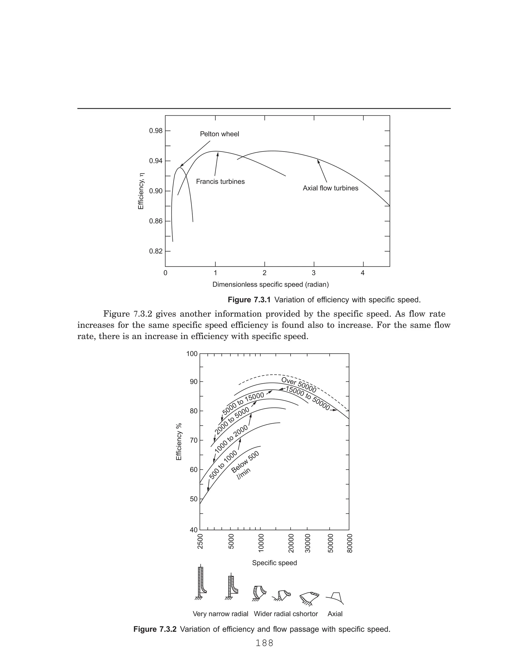
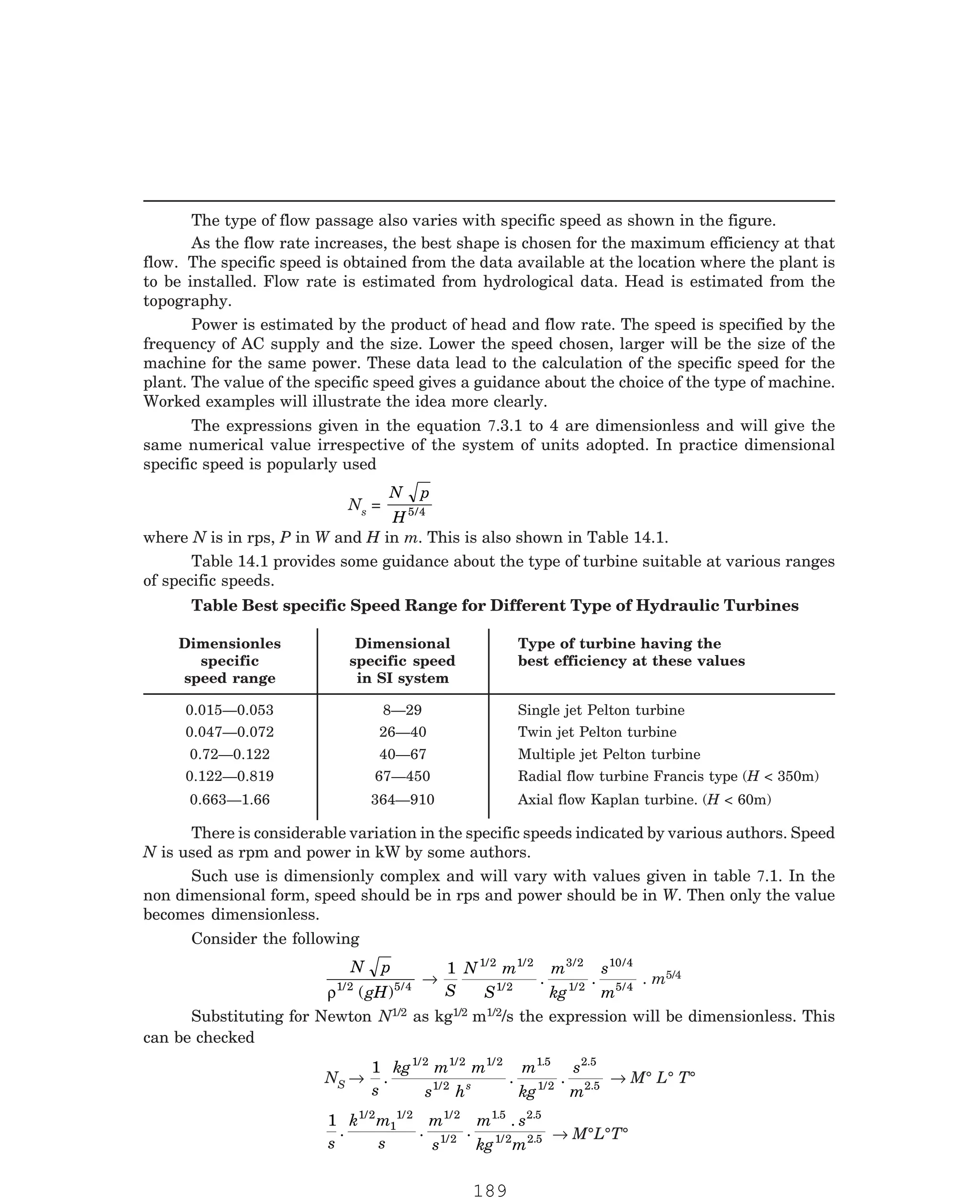
![P-2D:N-fluidFlu14-1.pm5
by the difference in pressure between the turbine entry and tailrace level. The following
efficiencies are generally used.
1. Hydraulic efficiency : It is defined as the ratio of the power produced by the turbine
runner and the power supplied by the water at the turbine inlet.
ηH =
Power produced by the runner
ρ Q g H
where Q is the volume flow rate and H is the net or effective head. Power produced by the
runner is calculated by the Euler turbine equation P = Qρ [u1 Vu1 – u2 Vu2]. This reflects the
runner design effectiveness.
2. Volumetric efficiency : It is possible some water flows out through the clearance
between the runner and casing without passing through the runner.
Volumetric efficiency is defined as the ratio between the volume of water flowing through
the runner and the total volume of water supplied to the turbine. Indicating Q as the volume
flow and ∆Q as the volume of water passing out without flowing through the runner.
ηv =
Q Q
Q
– ∆
To some extent this depends on manufacturing tolerances.
3. Mechanical efficiency : The power produced by the runner is always greater than
the power available at the turbine shaft. This is due to mechanical losses at the bearings,
windage losses and other frictional losses.
ηm =
Power available at the turbine shaft
4. Overall efficiency : This is the ratio of power output at the shaft and power input by
the water at the turbine inlet.
η0 =
Power available at the turbine shaft
ρ QgH
Also the overall efficiency is the product of the other three efficiencies defind
η0 = NH Nm Nv
The fluid velocity at the turbine entry and exit can have three components in the tangential,
axial and radial directions of the rotor. This means that the fluid momentum can have three
components at the entry and exit. This also means that the force exerted on the runner can
have three components. Out of these the tangential force only can cause the rotation of
the runner and produce work. The axial component produces a thrust in the axial direction,
which is taken by suitable thrust bearings. The radial component produces a bending of the
shaft which is taken by the journal bearings.
(7.4.3)
Power produced by the runner
7.5 EULER TURBINE EQUATION
195](https://image.slidesharecdn.com/hydraulicturbines2-251114192057-bc3f4363/75/HYDRAULIC-TURBINES-with-question-and-answer-pdf-10-2048.jpg)
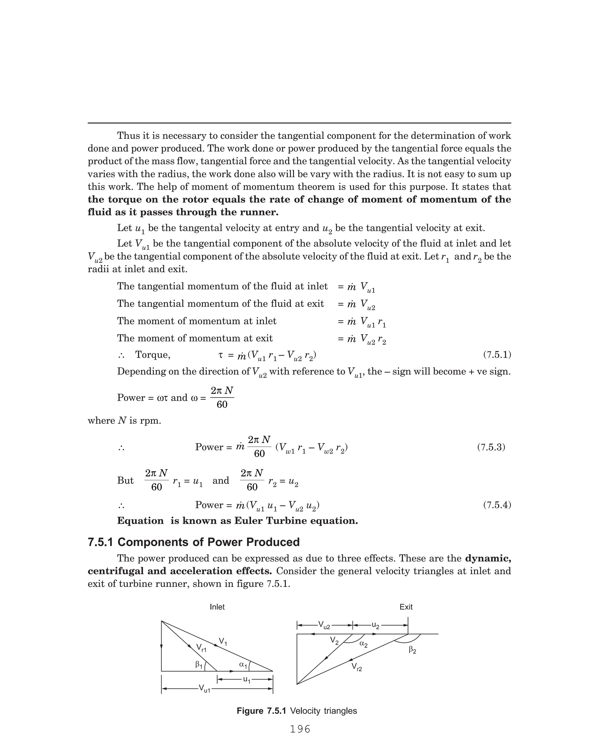
![P-2D:N-fluidFlu14-1.pm5
V1, V2 Absolute velocities at inlet and outlet.
Vr1, Vr2 Relative velocities at inlet and outlet.
u1, u2 Tangential velocities at inlet and outlet.
Vu1, Vu2 Tangential component of absolute velocities at inlet and outlet.
From inlet velocity triangle, (Vu1 = V1 cos α1)
Vr1
2 = V1
2 + u1
2 – 2u1 V1 cos α1
or u1 V1 cos α1 = Vu1 u1 =
V u vr
1
2
1
2
1
2
2
+ −
(A)
From outlet velocity triangle (Vu2 = V2 cos α2)
Vr2
2 = V2
2 + u2
2 – 2 u2 V2 cos α2
or u2 V2 cos α2 = u2 Vu2 = (V2
2 – u2
2 + Vr2
2)/2 (B)
Substituting in Euler equation,
Power per unit flow rate (here the Vu2 is in the opposite to Vu1)
m(u1 Vu1 + u2 Vu2) =
m
1
2
[(V1
2 – V2
2) + (u1
2 – u2
2) + (Vr2
2 – Vr1
2)]
V V
1
2
2
2
2
−
is the dynamic component of work done
u u
1
2
2
2
2
−
is the centrifugal component of work and this will be present only in the
radial flow machines
u V
r r
2
2
1
2
2
−
is the accelerating component and this will be present only in the reaction
turbines.
The first term only will be present in Pelton or impulse turbine of tangential flow
type.
In pure reaction turbines, the last two terms only will be present.
In impulse reaction turbines of radial flow type, all the terms will be present. (Francis
turbines is of this type).
In impulse reaction turbines, the degree of reaction is defined by the ratio of energy
converted in the rotor and total energy converted.
R =
( – ) ( – )
( – ) ( – ) ( – )
u u V V
V V u u V V
r r
r r
1
2
2
2
2
2
1
2
1
2
2
2
1
2
2
2
2
2
1
2
+
+ +
The degree of reaction is considered in detail in the case of steam turbines where speed
reduction is necessary. Hydraulic turbines are generally operate of lower speeds and hence
degree of reaction is not generally considered in the discussion of hydraulic turbines.
197](https://image.slidesharecdn.com/hydraulicturbines2-251114192057-bc3f4363/75/HYDRAULIC-TURBINES-with-question-and-answer-pdf-12-2048.jpg)
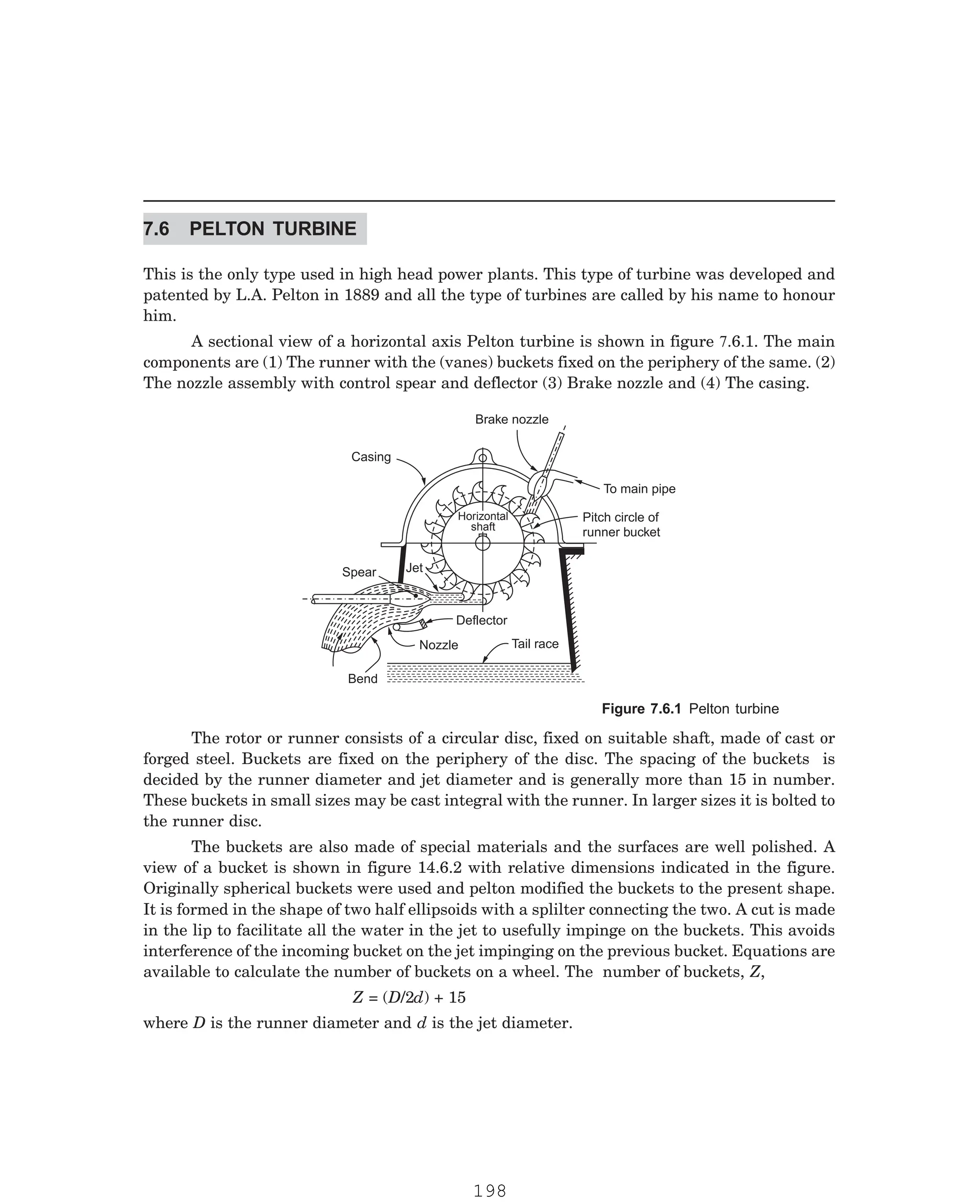
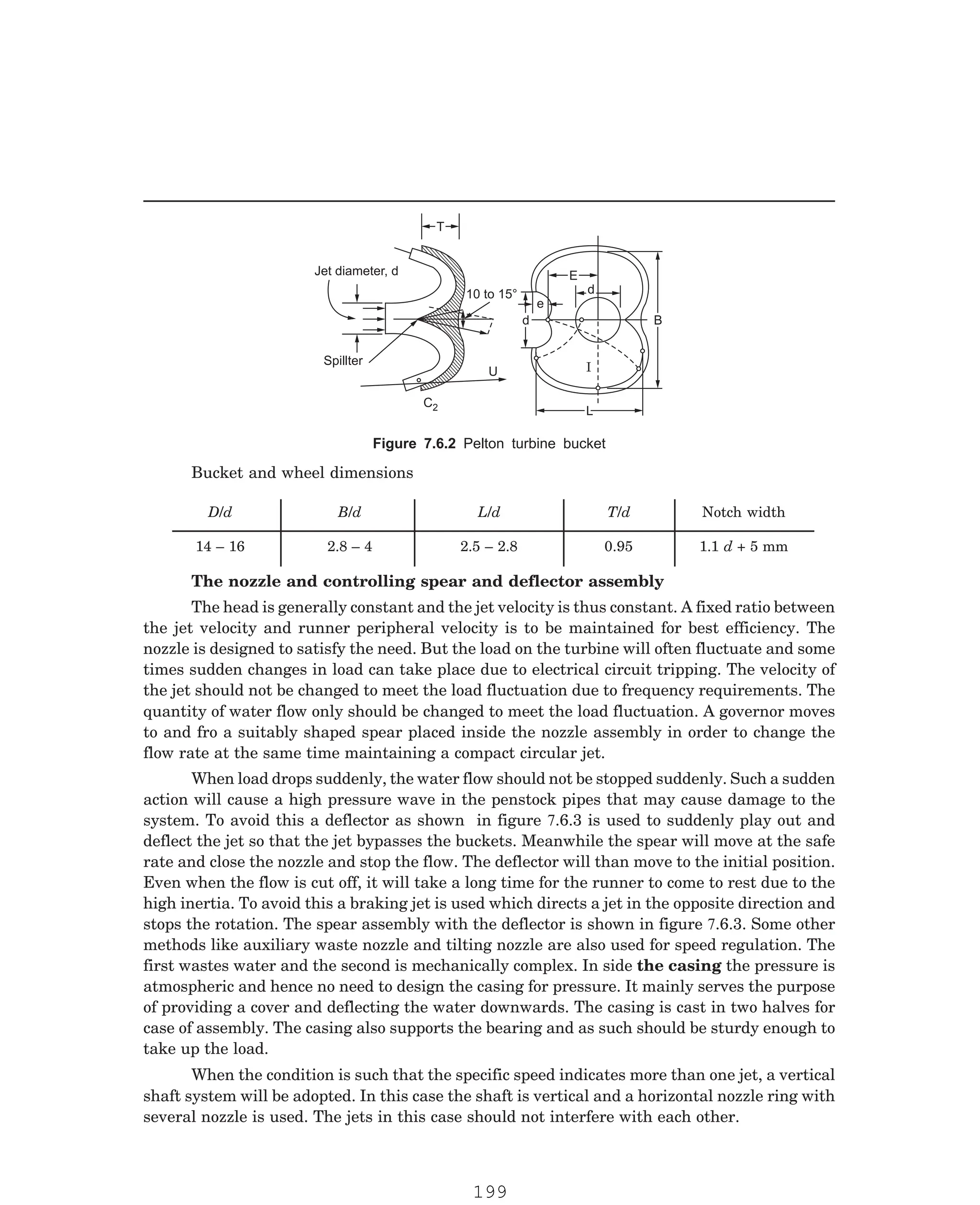
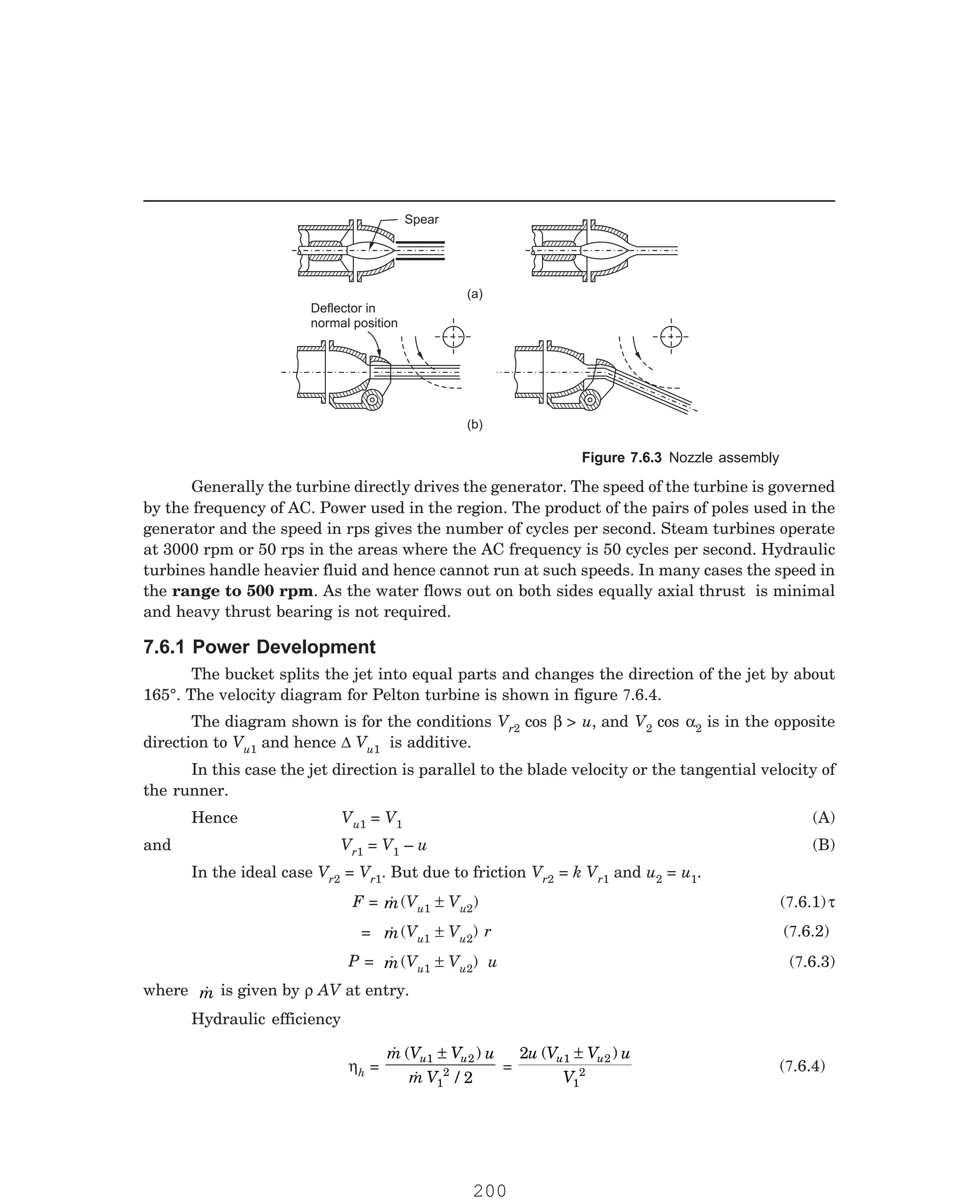
![P-2D:N-fluidFlu14-1.pm5
Once the effective head of turbine entry is known V1 is fixed given by V1 = C gH
v 2 . For
various values of u, the power developed and the hydraulic efficiency will be different. In fact
the out let triangle will be different from the one shown it u Vr2 cos β. In this case Vu2 will be
in the same direction as Vu1 and hence the equation (14.6.3) will read as
P =
m (Vu1 – Vu2) u
It is desirable to arrive at the optimum value of u for a given value of V1
V = Vu1
1
u
u
Vr1
Vr1 u b2
a2
Vu2
Vr2
Vu2
u
Vr2
V2
b2
Alternate exit triangle
u V cos b2
r2
Vu2
V2
u
u
V2
u1 = V1, Vu2 = Vr2 cos β2 – u = kVr1 cos β2 – u = k(V1 – u) cos β2 – u
∴ Vu1 + Vu2 = V1 + k V1 cos β2 – u cos β2 – u
= V1 (1 + k cos β2) – u(1 + k cos β2)
= (1 + k cos β2) (V1 + u)
Substituting in equation (14.6.4)
ηH =
2
1
2
u
V
× (1 + k cos β2) (V1
= 2(1 + k cos β2) u
V
u
V
1
2
1
2
–
L
NMM
O
QPP
u
V1
is called speed ratio and denoted as φ.
∴ ηH = 2(1 + k cos β2) [φ – φ2
and equated to zero.
d
d
H
η
φ
= 2(1 + k cos β2) (1 – 2 φ)
∴ φ =
u
V1
=
1
2
or u = 0.5 V1
In practice the value is some what lower at u = 0.46 V1
Substituting equation (14.6.6) in (14.6.4a) we get
ηH = 2(1 + k cos β2) [0.5 – 0.52]
. Equation 7.6.4
can be modified by using the following relations.
Figure 7.6.4 Velocity triangles Pelton turbine
V
+ u) (7.6.4a)
] (7.6.5)
To arrive at the optimum value of φ, this expression is differentiated with respect to φ
201](https://image.slidesharecdn.com/hydraulicturbines2-251114192057-bc3f4363/75/HYDRAULIC-TURBINES-with-question-and-answer-pdf-16-2048.jpg)
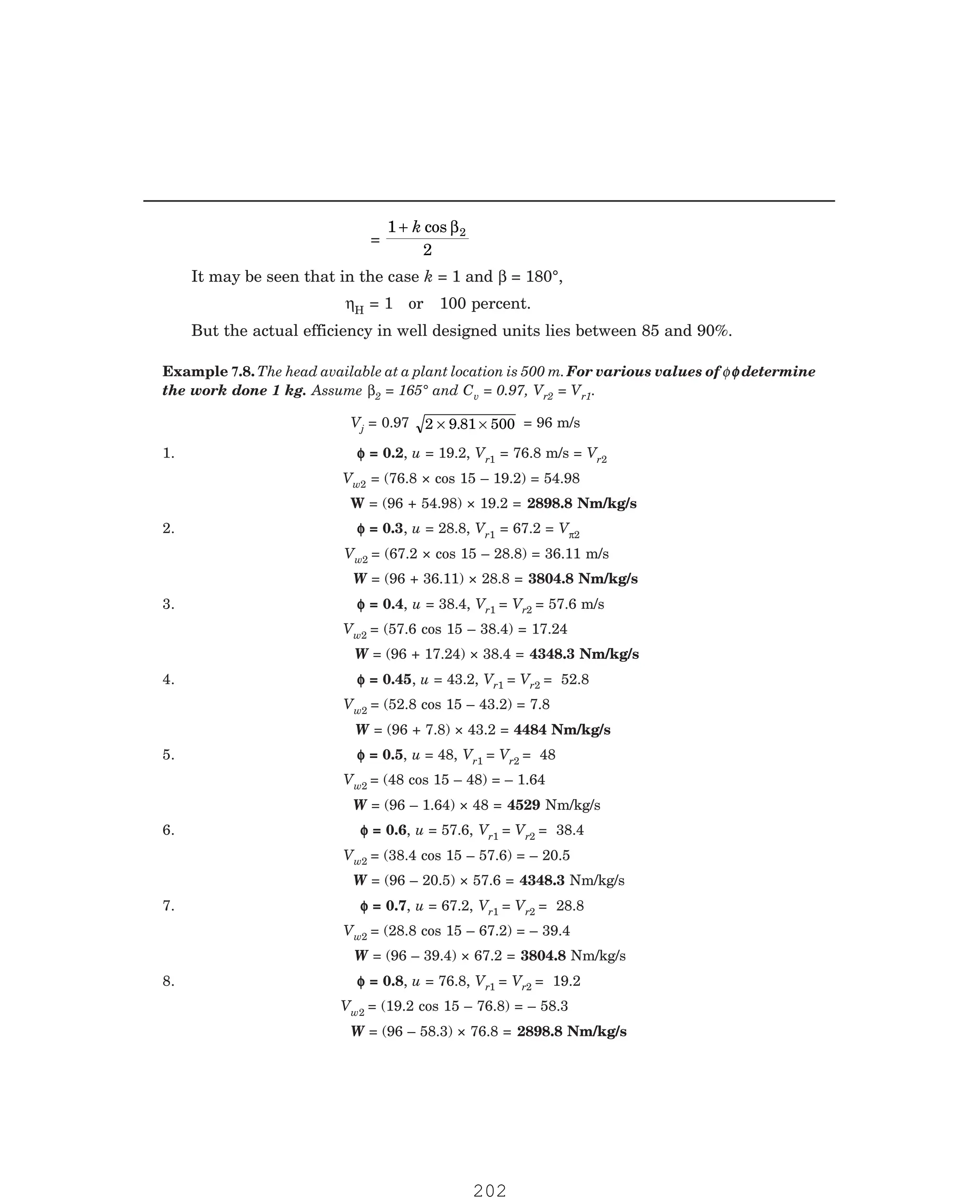
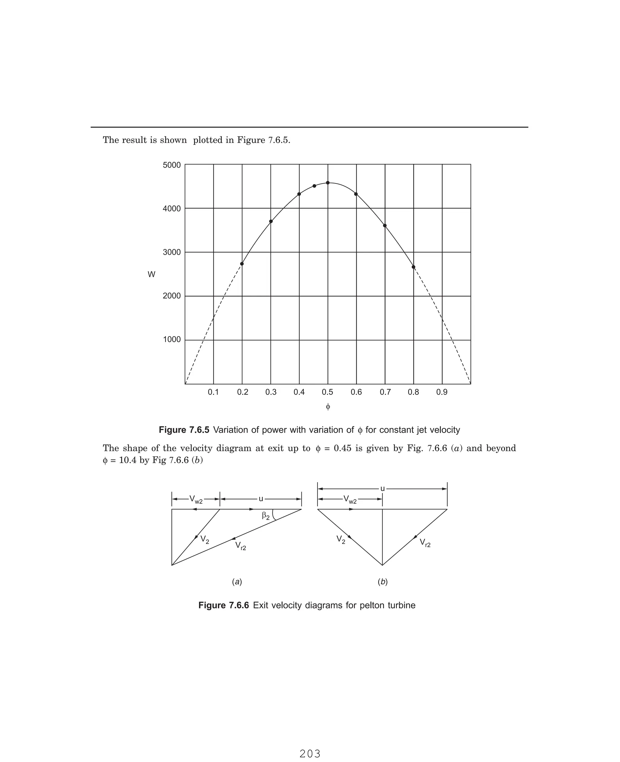
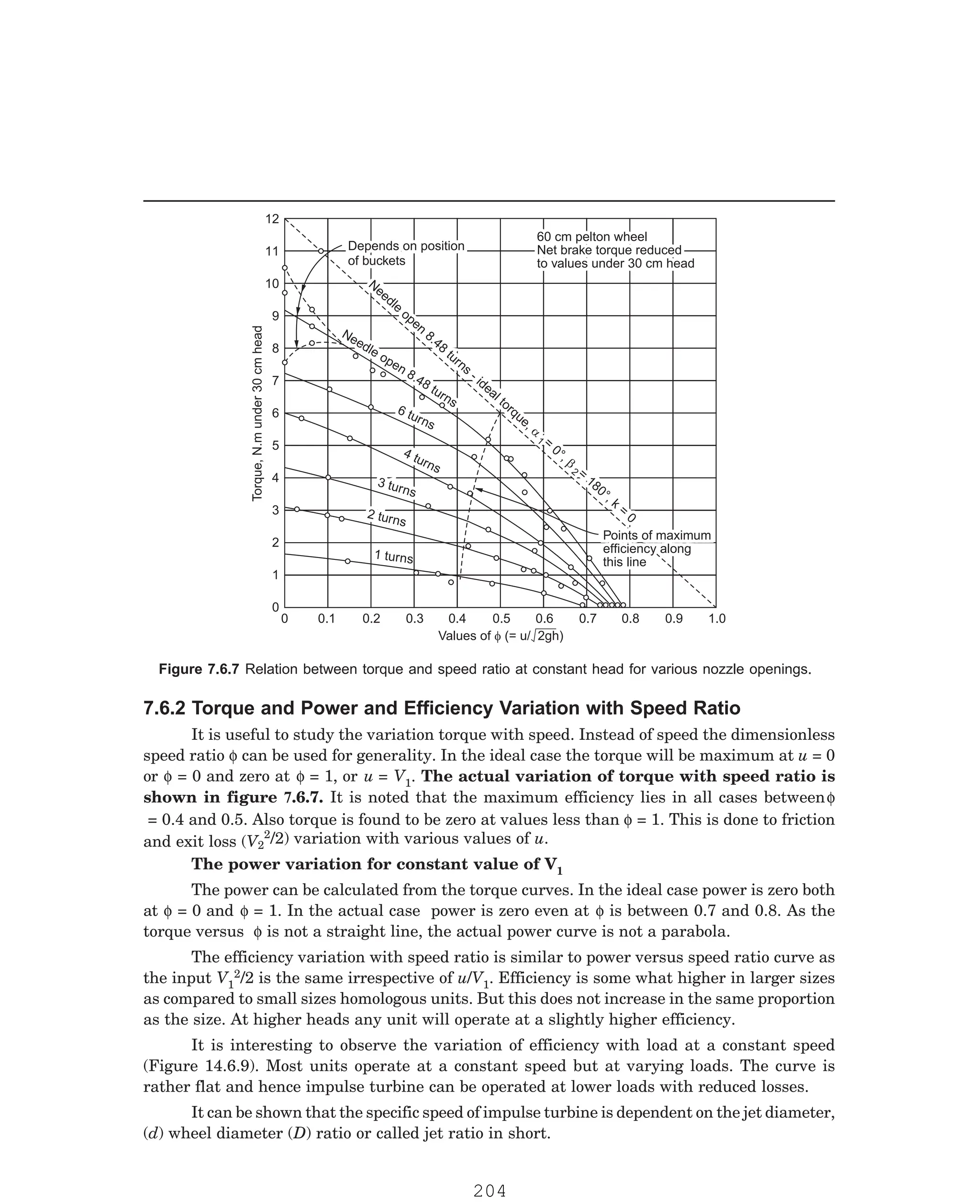
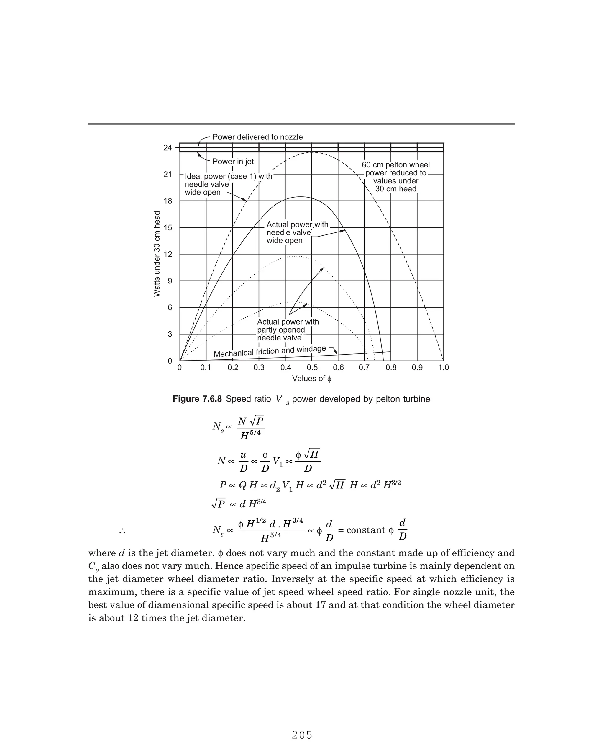
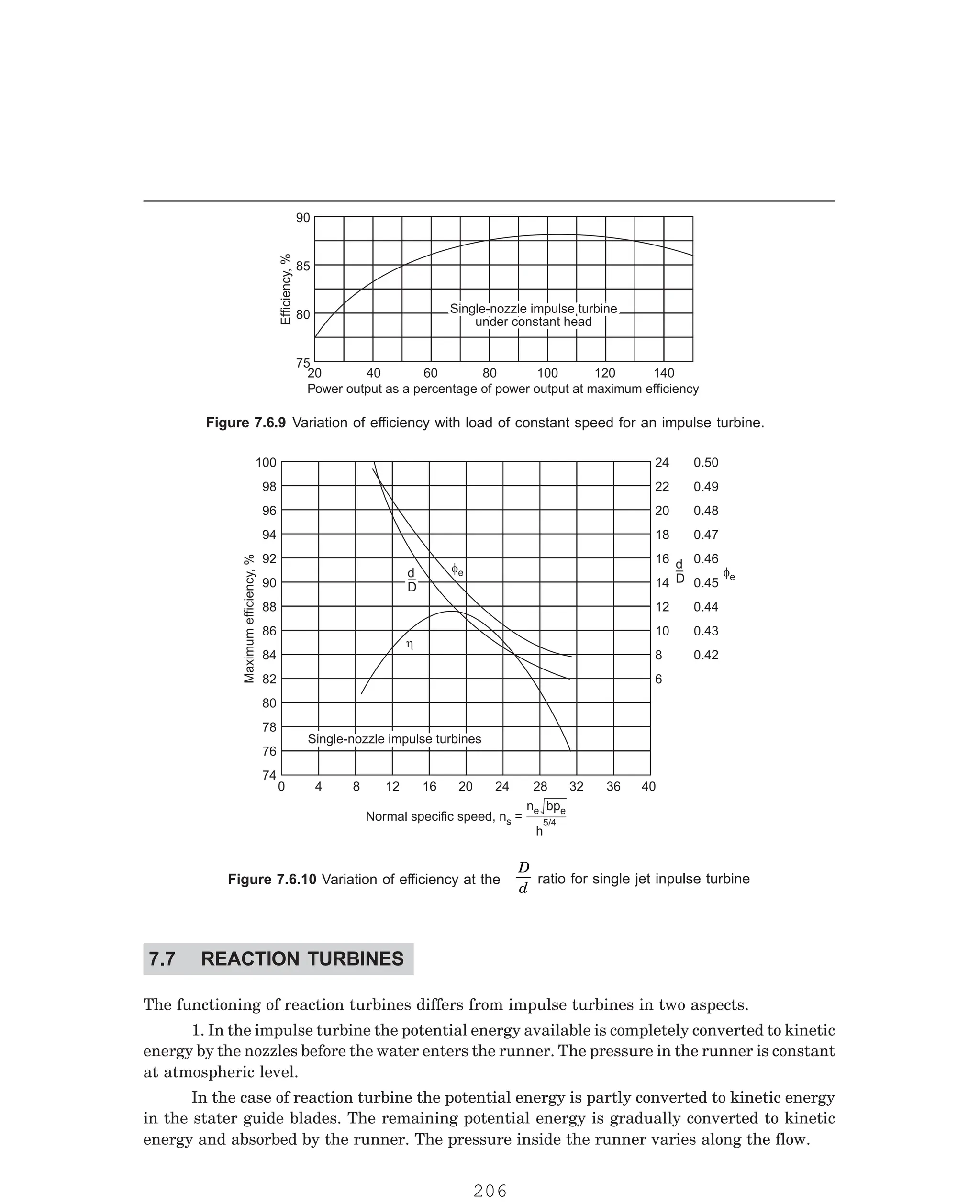
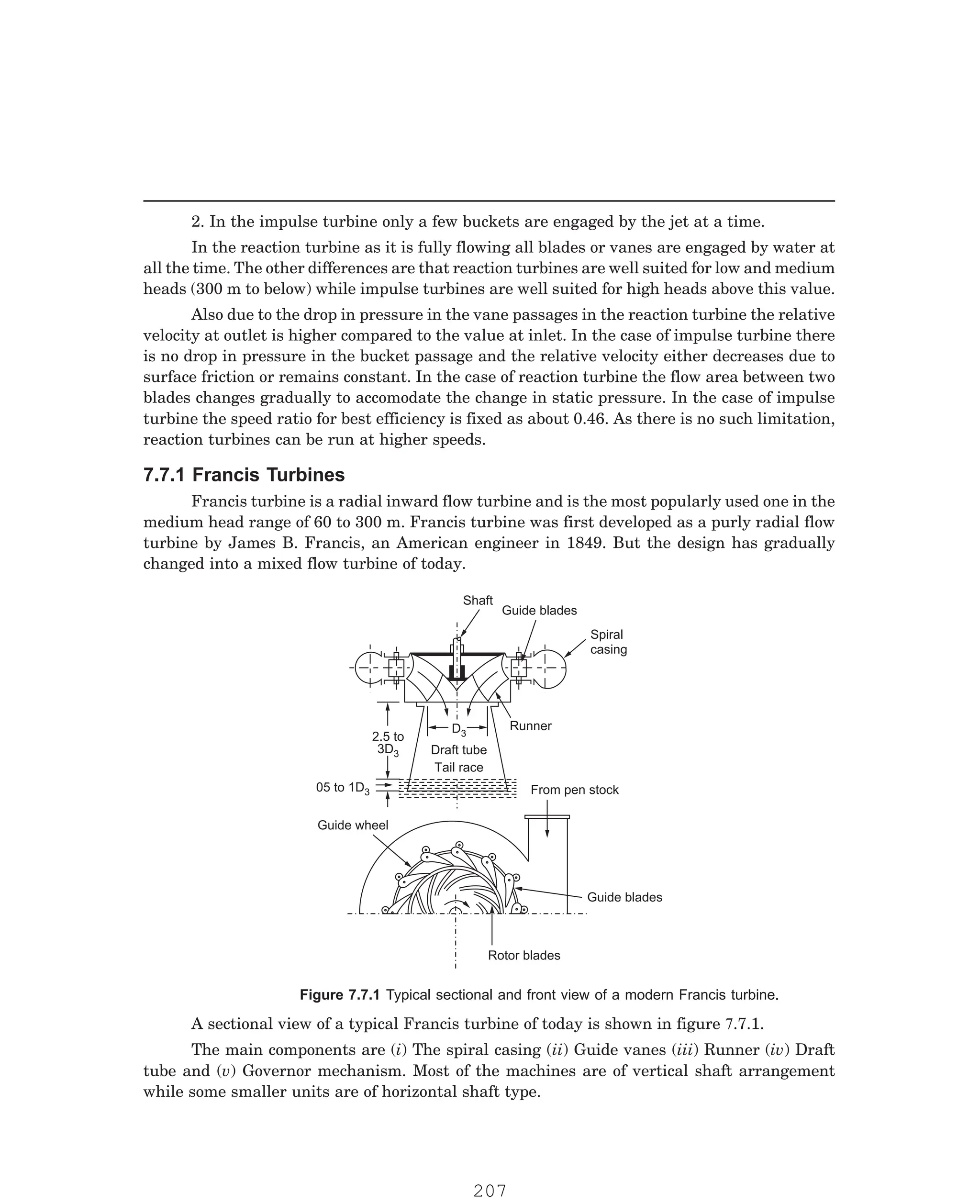
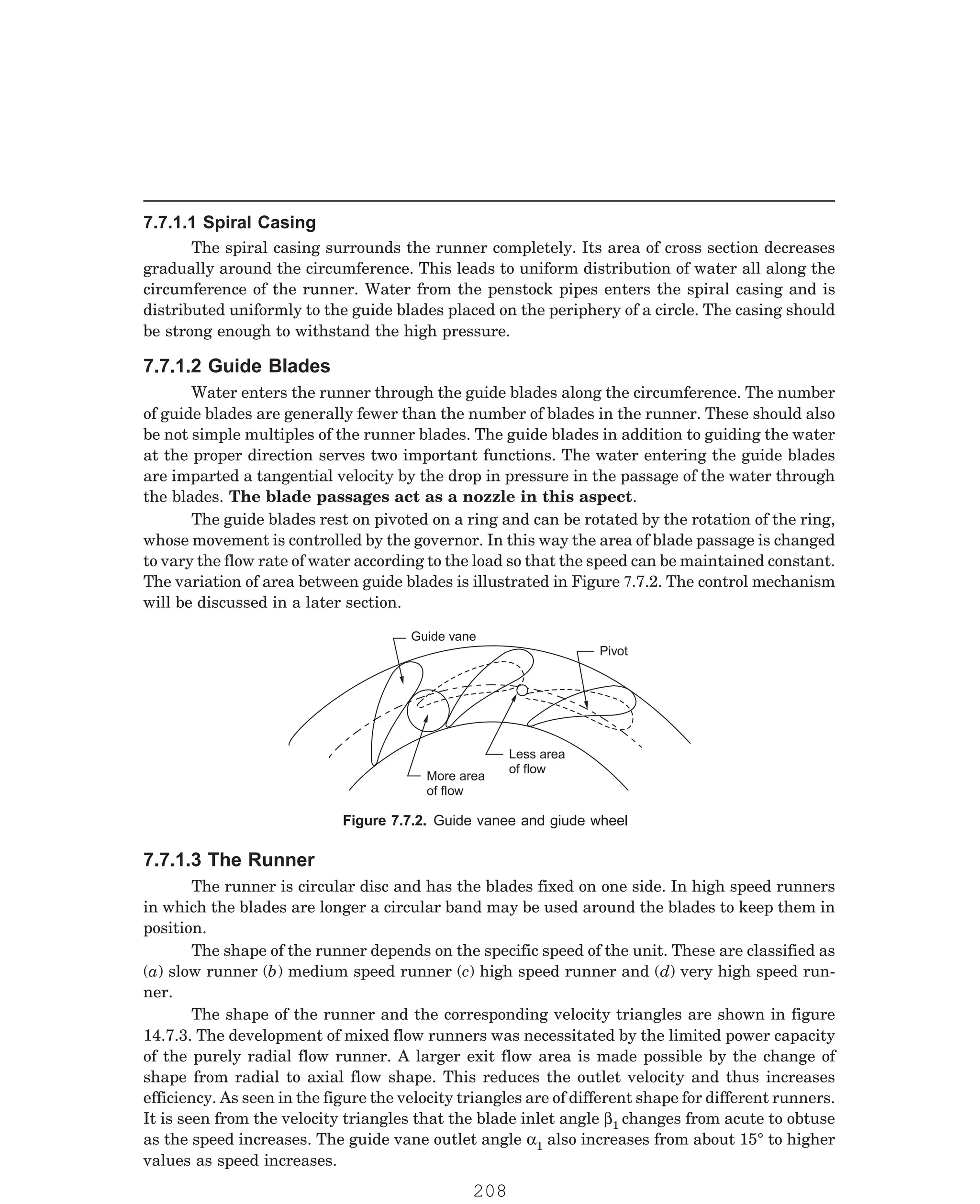
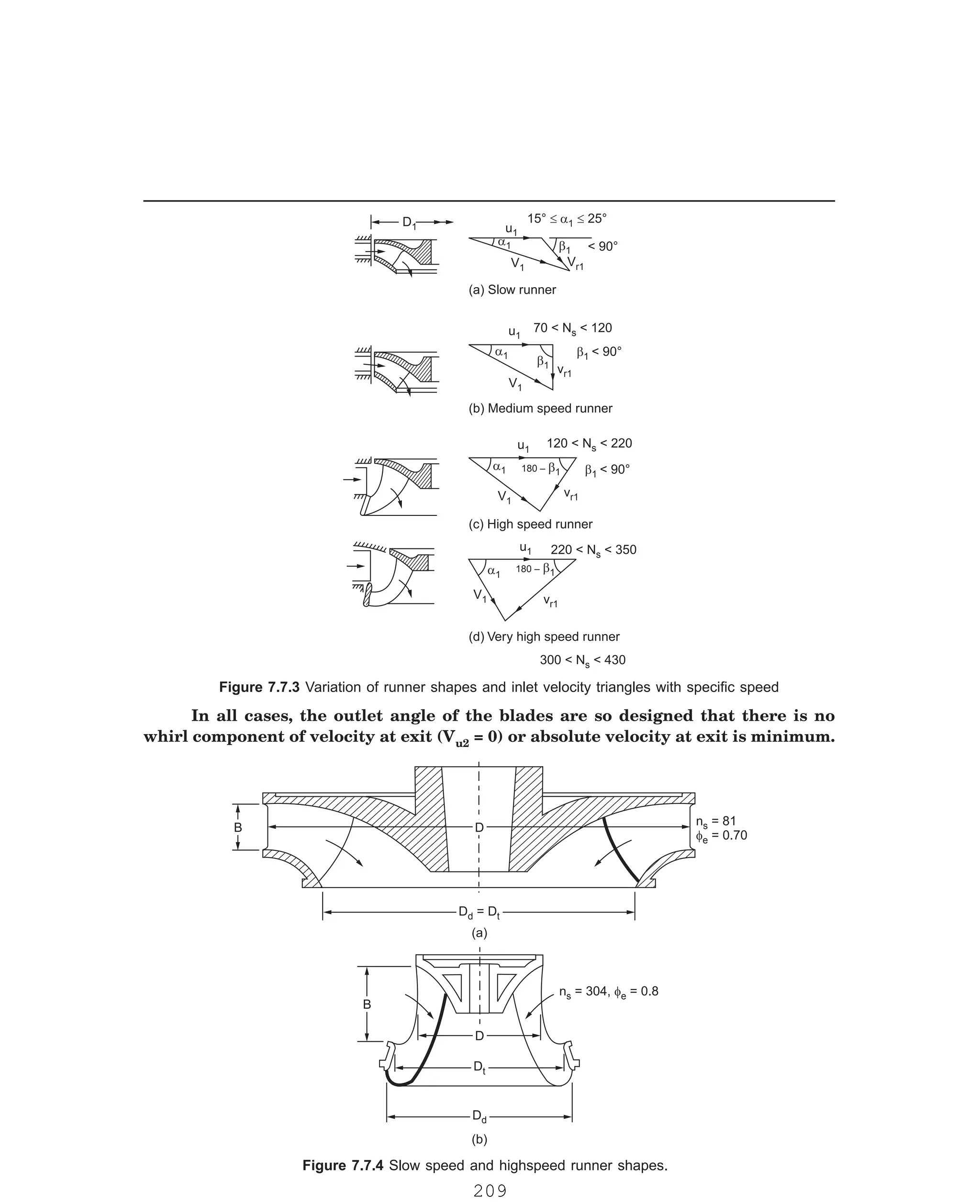
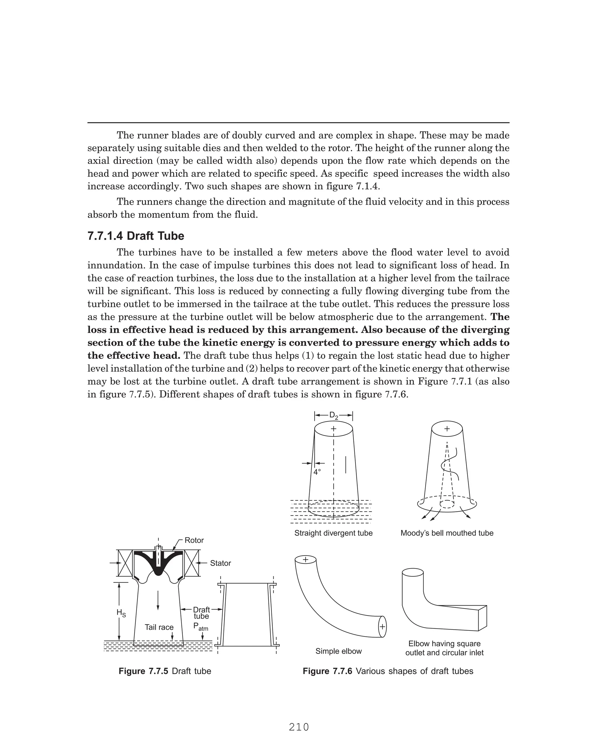
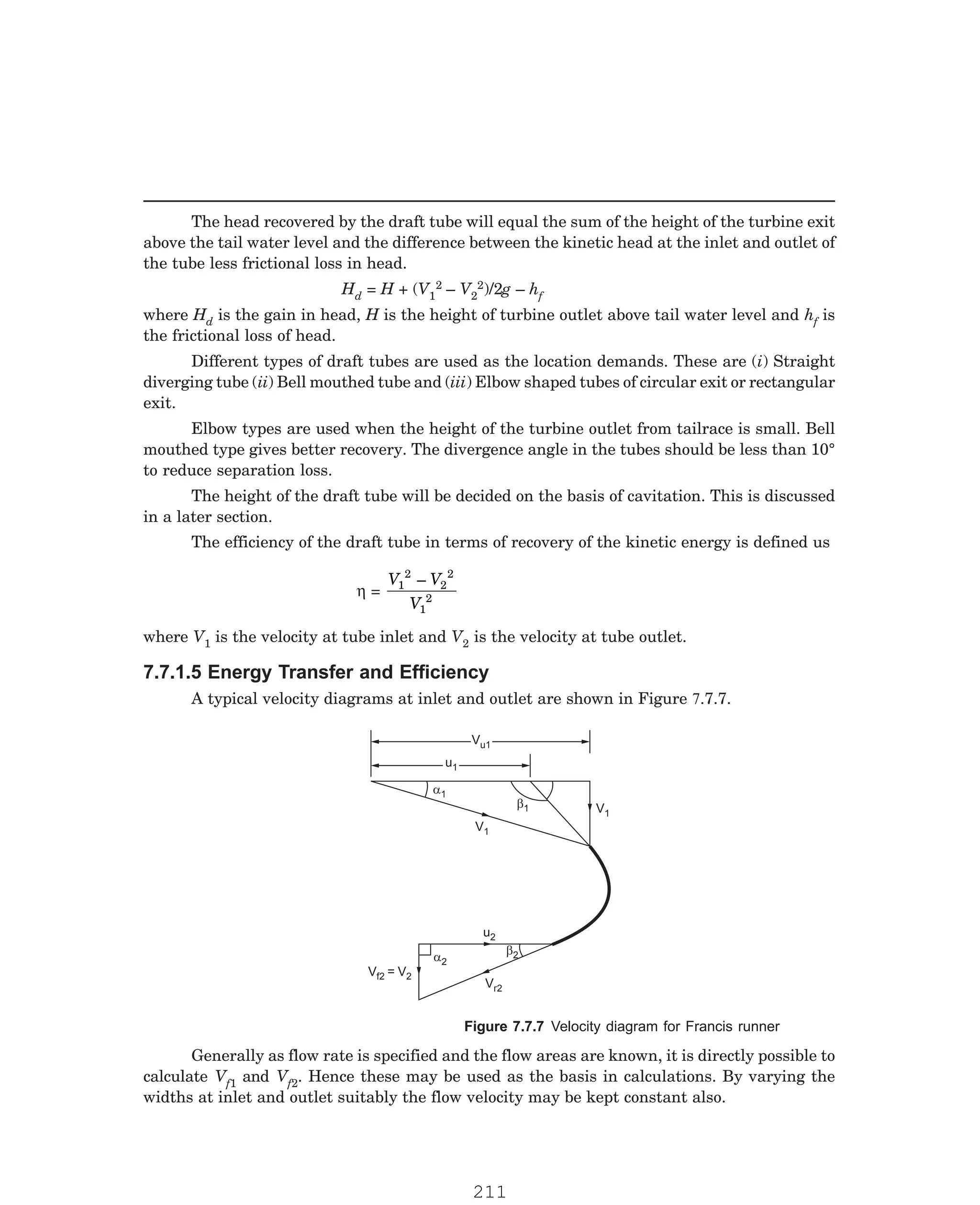
![P-2D:N-fluidFlu14-2.pm5
u1 = Vf [cot α1 + cot β1]
∴ u1Vu1 = Vf1
2 cot α1 [cot α1 + cot β1]
Energy supplied to the runner is
u1 Vu1 +
V2
2
2
= u1 Vu1 +
Vf 2
2
2
= u1 Vu1 +
Vf 1
2
2
(Assume Vf2 = Vf1)
∴ ηb=
V
V
V
f
f
f
1
2
1 1 1
1
2
1
2
1 1 1
2
cot [cot cot ]
cot [cot cot ]
α α β
α α β
+
+ +
Multiply by 2 and add and subtract Vf1
2 in the numerator to get
ηb= 1 –
1
1 2 1 1 1
+ +
cot (cot cot )
α α β
In case β
β
β
β
β1 = 90°
ηb= 1 –
1
1
2
2
1
+
tan α
=
2
2 2
1
+ tan α
In this case Vu1 = u1
100
80
60
40
20
0
50
40
30
20
10
0
600
500
400
300
200
100
0
Water
Power
=
Power
Input
(kW)
Value
of
h
(m)
Brake Power = Power output (kW)
0 500
50 100 150 200 250 300 350 400 450
Head
Head
Efficiency
Efficiency
Power input
Power input
n = 600 rpm
n = 600 rpm
The efficiency curve is not as flat as that of impulse turbine. At part loads the efficiency
is relatively low. There is a drop in efficiency after 100% load.
The characteristics of Francis turbine is shown in Figure 7.7.8.
213](https://image.slidesharecdn.com/hydraulicturbines2-251114192057-bc3f4363/75/HYDRAULIC-TURBINES-with-question-and-answer-pdf-28-2048.jpg)
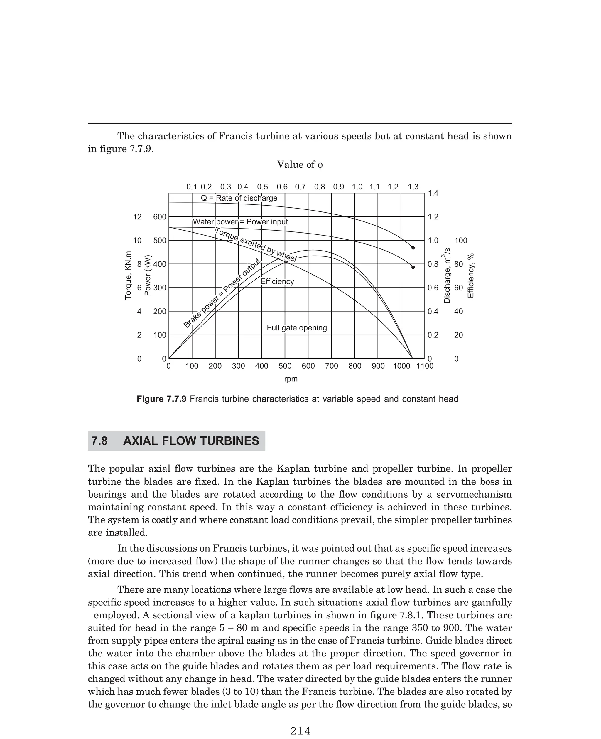
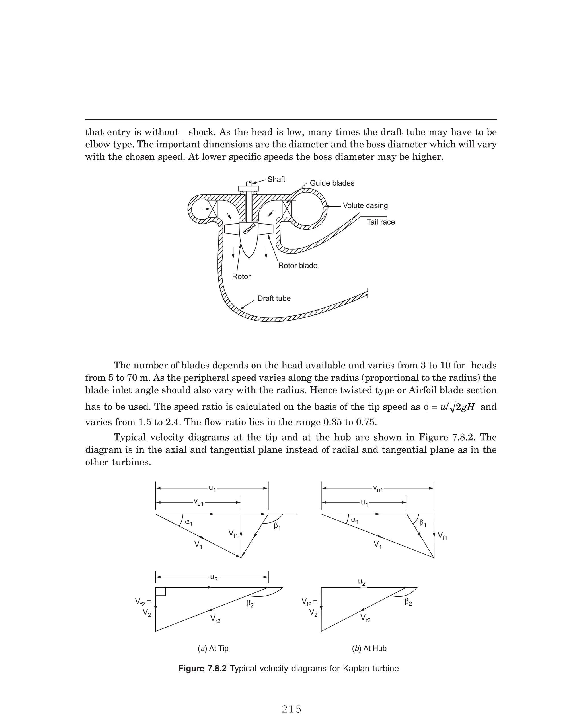
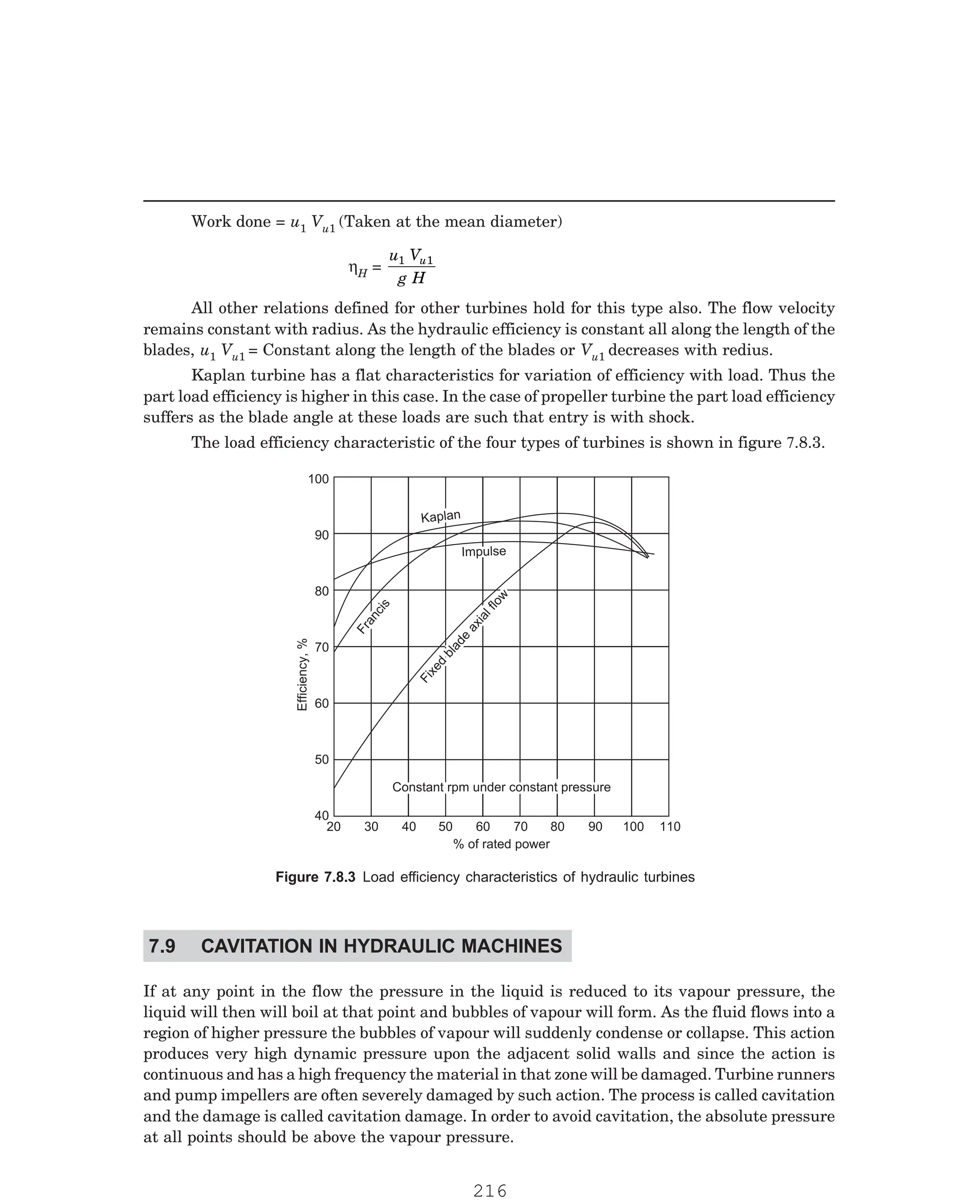
![P-2D:N-fluidFlu14-2.pm5
Cavitation can occur in the case of reaction turbines at the turbine exit or draft tube
inlet where the pressure may be below atmospheric level. In the case of pumps such damage
may occur at the suction side of the pump, where the absolute pressure is generally below
atmospheric level.
In addition to the damage to the runner cavitation results in undesirable vibration noise
and loss of efficiency. The flow will be disturbed from the design conditions. In reaction turbines
the most likely place for cavitation damage is the back sides of the runner blades near their
trailing edge. The critical factor in the installation of reaction turbines is the vertical distance
from the runner to the tailrace level. For high specific speed propeller units it may be desirable
to place the runner at a level lower than the tailrace level.
To compare cavitation characteristics a cavitation parameter known as Thoma cavitation
coefficient, σ, is used. It is defined as
σ =
h h z
h
a r
where ha is the atmospheric head hr is the vapour pressure head, z is the height of the runner
outlet above tail race and h is the total operating head. The minimum value of σ at which
cavitation occurs is defined as critical cavitation factor σe. Knowing σc the maximum value of
z can be obtained as
z = ha – hv – σe
c is found to be a function of specific speed. In the range of specific speeds for Francis
turbine σc varies from 0.1 to 0.64 and in the range of specific speeds for Kaplan turbine σc
varies from 0.4 to 1.5. The minimum pressure at the turbine outlet, h0 can be obtained as
h0 = ha – z – σc
There are a number of correlations available for the value of σc in terms of specific
speed, obtained from experiments by Moody and Zowski. The constants in the equations depends
on the system used to calculate specific speed.
For Francis runners σc = 0.006 + 0.55 (Ns/444.6)1.8
c = 0.1 + 0.3 [Ns/444.6]2.5
Francis runner σc = 0.625
Ns
380 78
2
.
L
NM O
QP
For Kaplan runner σc = 0.308 +
1
6 82 380 78
2
. .
Ns
F
HG I
K
z = Pa – Pv – σc h = 8.6 – 0.17 – 0.3 × 20 = 2.43 m.
The turbine outlet can be set at 2.43 m above the tailrace level.
− −
(7.8.1)
h (7.8.2)σ
H (7.8.3)
(7.8.4)
For Kaplan runners σ (7.8.5)
Other empirical corrlations are
J (7.8.7)
Example 7.9. The total head on a Francis turbine is 20 m. The machine is at an elevation where
the atmosphic pressure is 8.6 m. The pressure corresponding to the water temperature of 15° C is
0.17 m. It critical cavitation factor is 0.3, determine the level of the turbine outlet above the tail race.
217](https://image.slidesharecdn.com/hydraulicturbines2-251114192057-bc3f4363/75/HYDRAULIC-TURBINES-with-question-and-answer-pdf-32-2048.jpg)
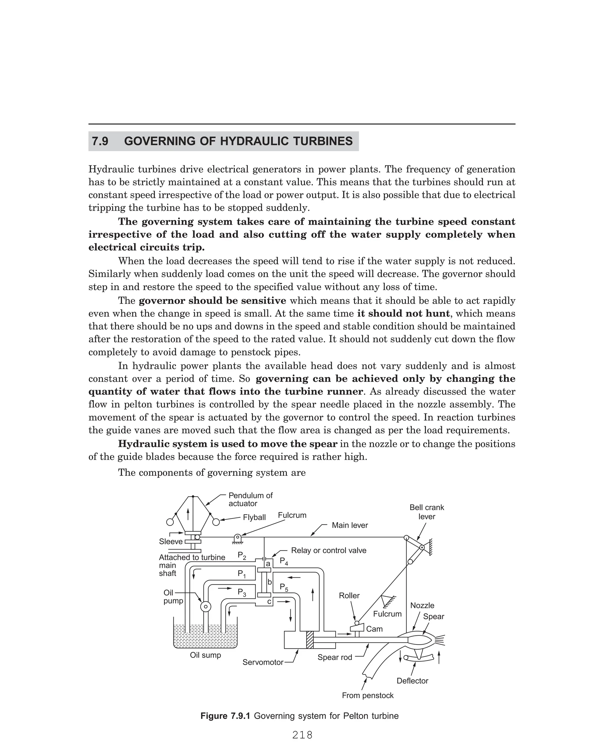
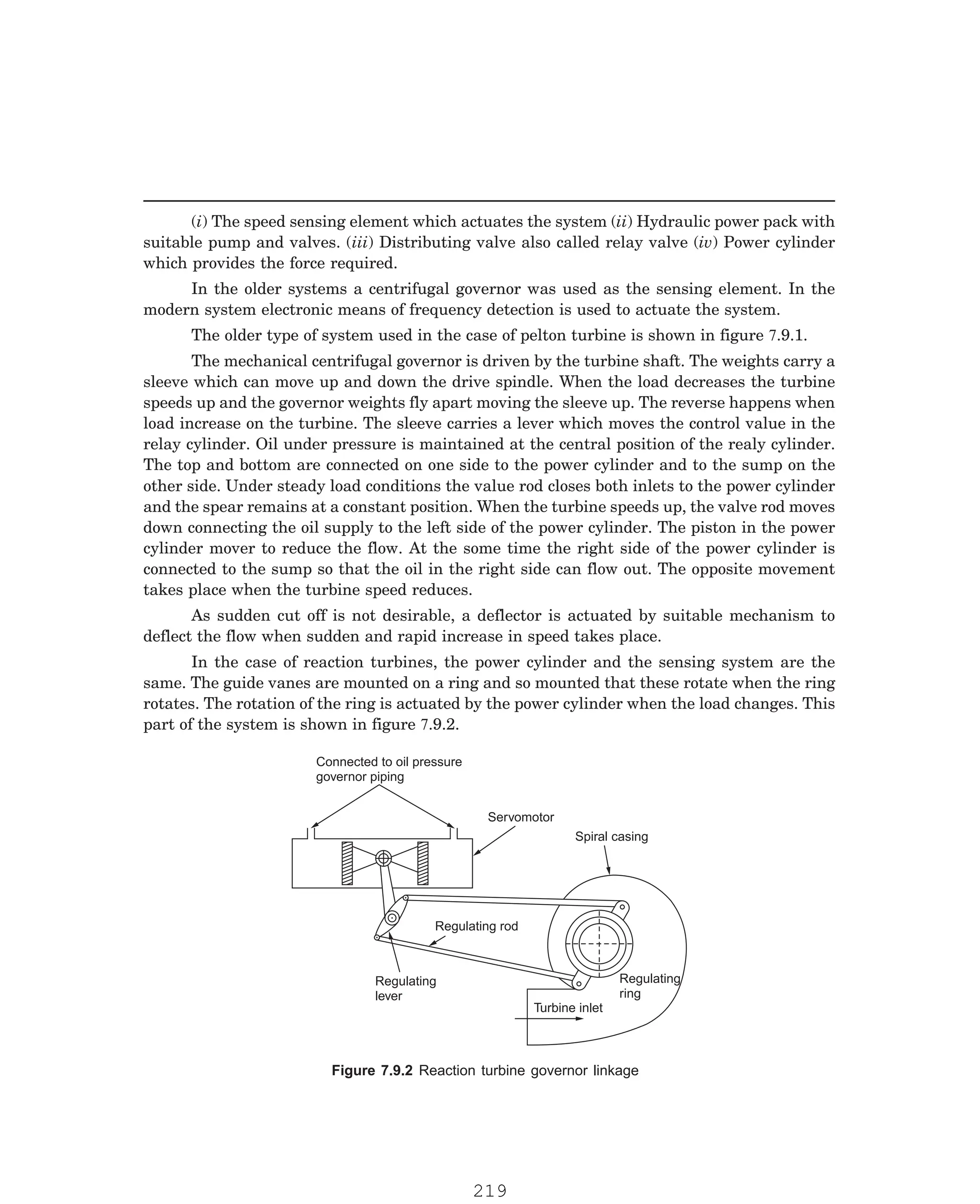
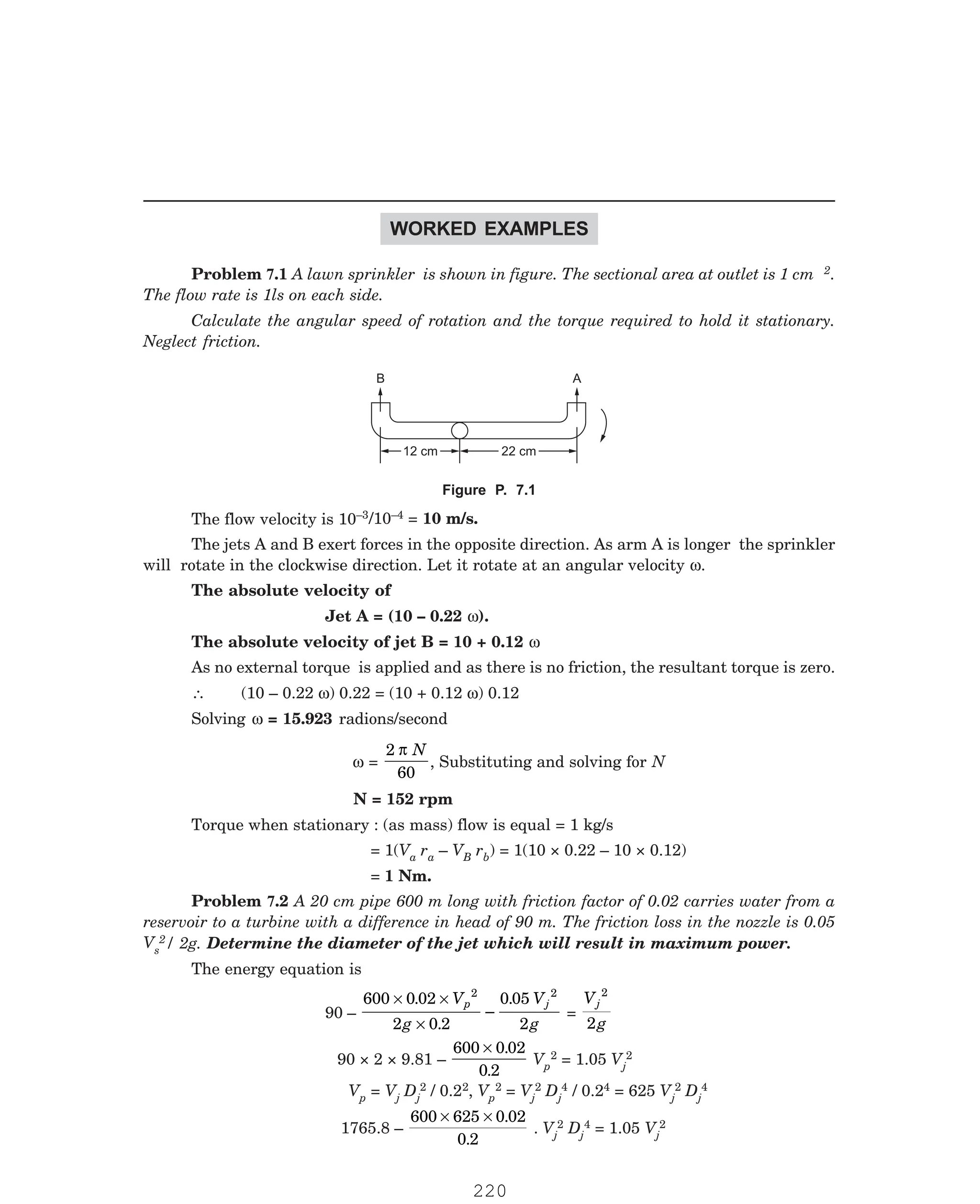
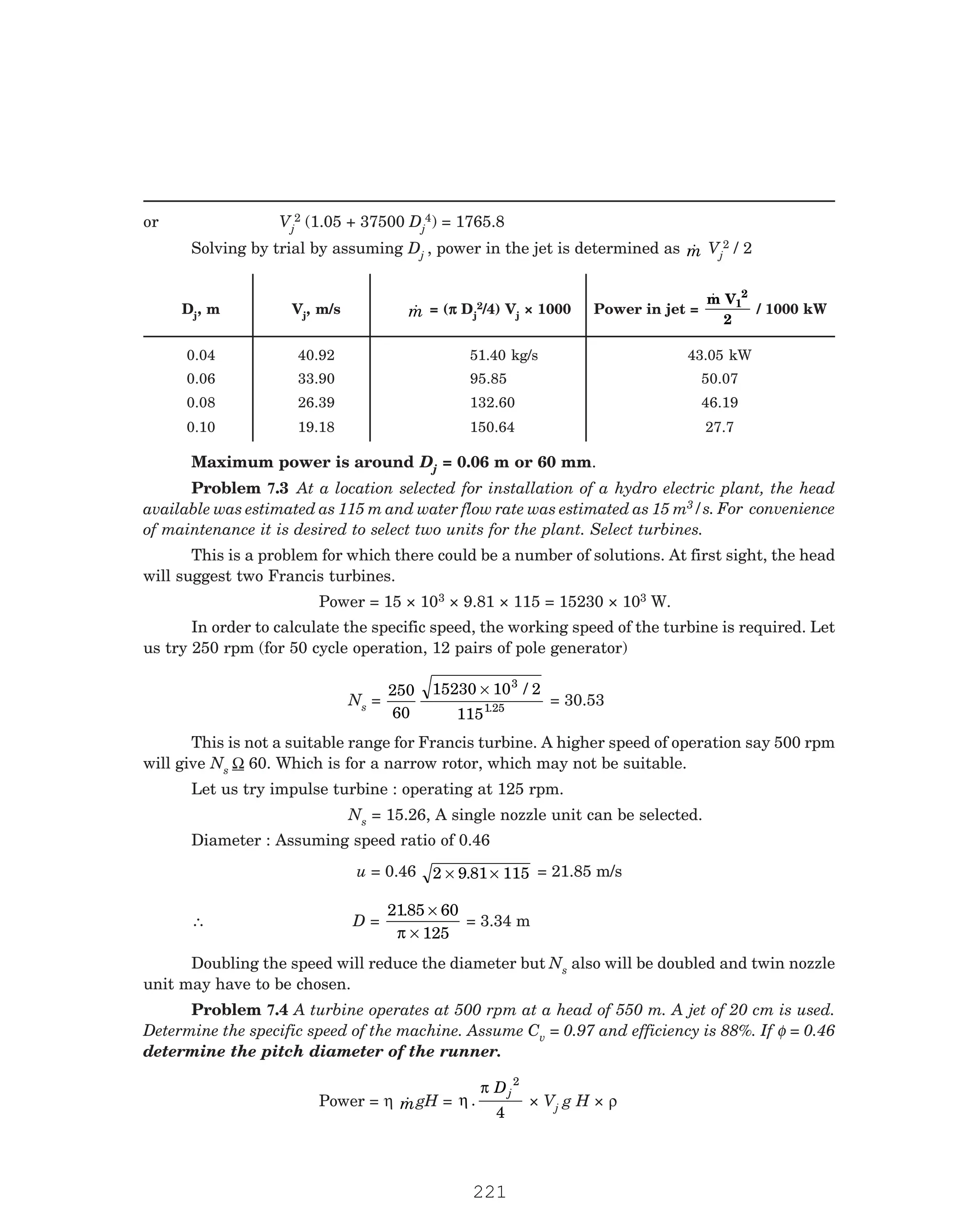
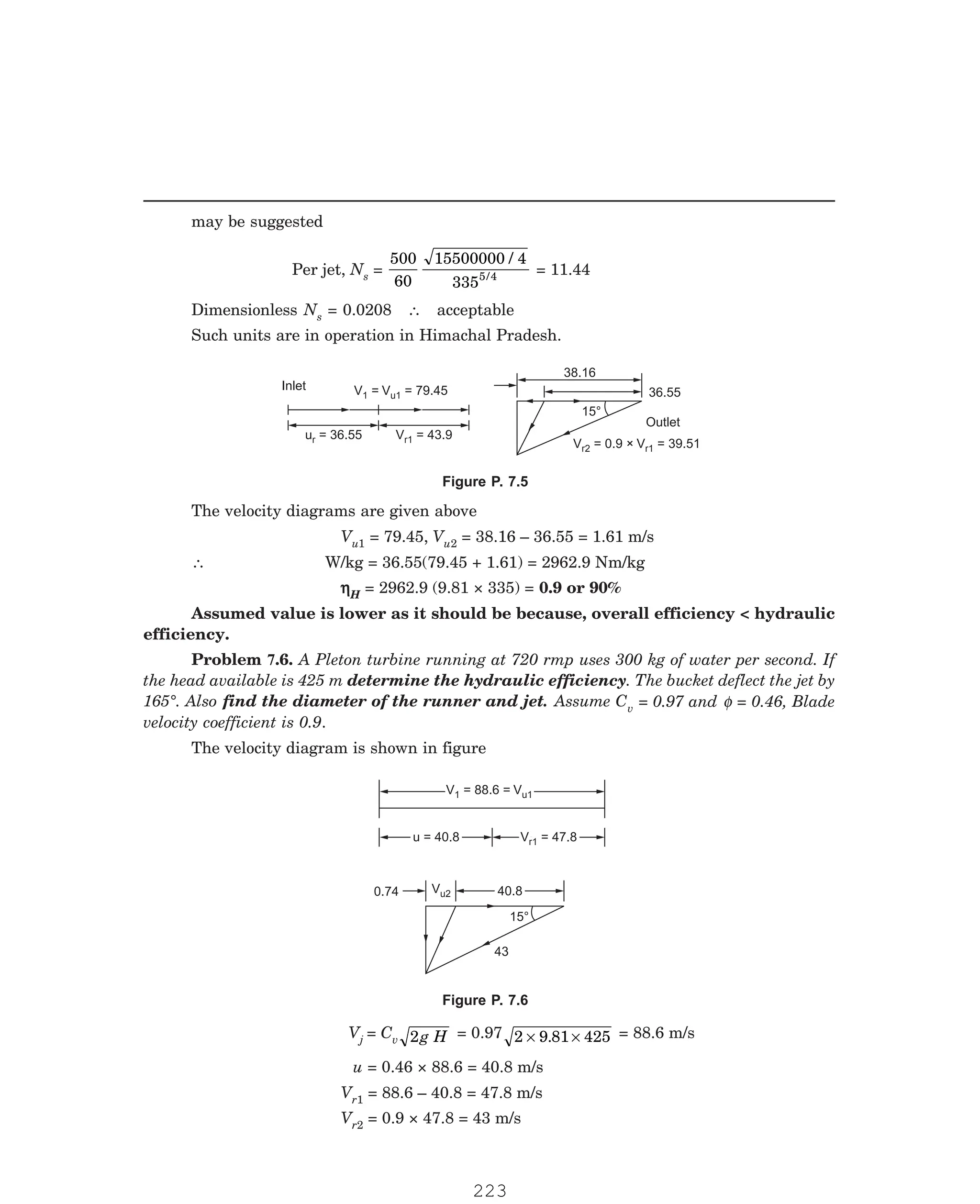
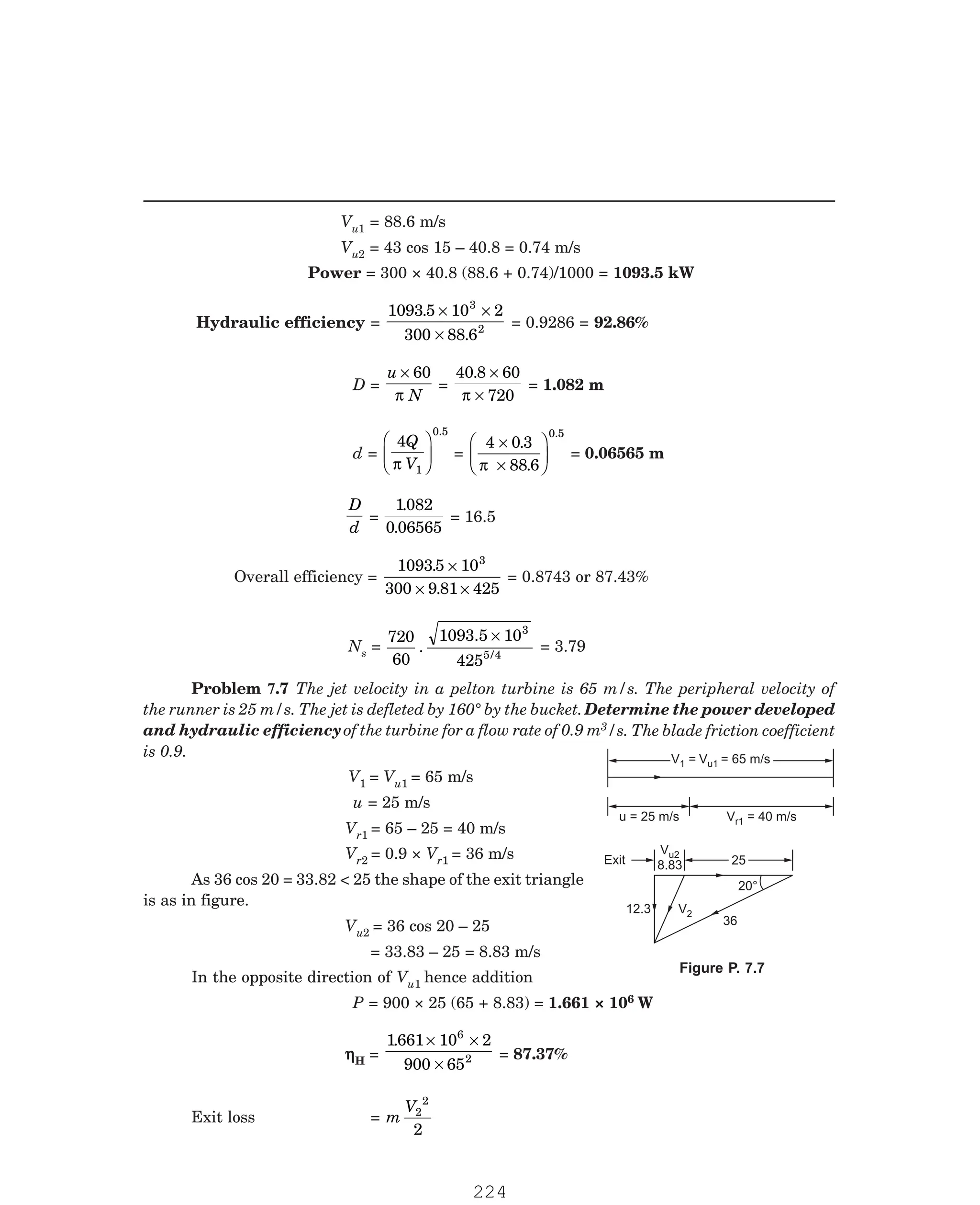
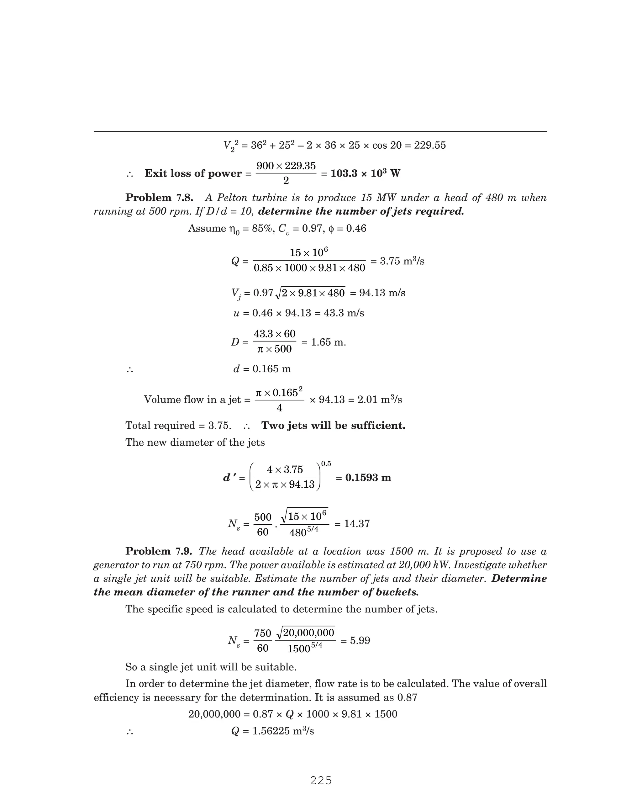
![P-2D:N-fluidFlu14-3.pm5
Jet diameter is found from flow rate and jet velocity.
πd2
4
× Vj = Q, d =
6 0372 4
76 43
0.5
.
.
×
×
L
NM O
QP
π
= 0.3171 m
Jet speed ratio is
D
d
= 12, ∴ D = 12 × 0.3171 = 3.8 m
The turbine rotor speed is determined from the tangential velocity
π DN
60
= u,
N =
u
D
× 60
π
= 35.16 × 60 / π × 3.8 = 176.71 rpm
Ns =
176.61
60
.
15 10
310
6
5/4
×
= 8.764
is 0.2096
d
D
, φ = 0.48, ηo = 90%, Cv = 0.98
Ns =
N P
gH
ρ1/2 5 4
( ) /
, where N is rps.
Q =
π d2
4
× Vj =
π d2
4
× 0.98 [2g H]1/2
= 3.4093 d2 H1/2
P = ηo × ρ g Q H = 0.9 × 1000 × 9.81 × 3.4093 d2 H1/2 × H
= 30100.73 d2 H1.5
N =
u
d
π
, u = 0.48 Vj = 0.48 × 0.98 2g H1/2 = 2.0836 H1/2
∴ N = 0.6632 H1/2 D – 1
∴ Ns =
0 6632 1/2
. H
D
[30100.73 d2H1.5]1/2 / 10001/2 g1.25 H1.25
= 115 068
1
.
.25
dH
D
/ 549 H1.25 = 0.2096
d
D
3/s. Total head is 115 m. For shockless
entry determine the angle of the inlet guide vane. Also find the absolute velocity at entrance, the
Problem 7.12. Show that for the following constants, the dimensionless specific speed
Problem 7.13. The outer diameter of a Francis runner is 1.4 m. The flow velocity at
inlet is 9.5 m/s. The absolute velocity at the exit is 7 m/s. The speed of operation is 430 rpm.
The power developed is 12.25 MW, with a flow rate of 12 m
228](https://image.slidesharecdn.com/hydraulicturbines2-251114192057-bc3f4363/75/HYDRAULIC-TURBINES-with-question-and-answer-pdf-43-2048.jpg)
![P-2D:N-fluidFlu14-3.pm5
runner blade angle at inlet and the loss of head in the unit. Assume zero whirl at exit. Also fluid
the specific speed.
The runner speed u1 =
π D N
60
=
π × ×
430 14
60
.
= 31.52 m/s
As Vu2 = 0,
Power developed =
m Vu1 u1
12.25 × 106 = 12 × 103 × Vu1 × 31.52
Solving Vu1 = 32.39 m/s
Vu1 u1
∴ The shape of the inlet
Velocity triangle is as given. Guide blade angle αr
tan α1 =
9 5
32 39
.
.
∴ α
α
α
α
α1 = 16.35°
V1 = (Vf1
2 + Vu1
2)0.5 = [9.52 + 32.392]0.5 = 33.75 m/s
Blade inlet angle β1
tan β1 = 9.5 / (32.39 – 31.52)
∴ β
β
β
β
β1 = 84.77°
Total head = 115 m. head equal for Euler work =
m Vu1 u1/g
=
32 39 3152
9 81
. .
.
×
= 104.07 m
Head loss in the absolute velocity at exit
=
7
2 9 81
2
× .
= 2.5 m
∴ Loss of head = 115 – 104.07 – 2.5 = 8.43 m
Ns =
430
60
12 25 10
115
6
1
.
.
.25
×
= 223.12
As the inner diameter is not known blade angle at outlet cannot be determined.
3/s . The exit velocity at the draft tube outlet is 16 m/s. Assuming zero whirl velocity at exit
and neglecting blade thickness determine the overall and hydraulic efficiency and rotor blade
angle at inlet. Also find the guide vane outlet angle :
Overall efficiency =
Power developed
Hydraulic power
=
16120 10
7 1000 9 81 260
3
×
× × ×
.
ηo = 0.9029 or 90.29%
V = 32.39 m/s
u1
V = 32.39 m/s
u1
u = 31.51
1
u = 31.51
1
a1 b1
V = 9.5 m/s
f1
Figure P. 7.13
Problem 7.14. A Francis turbine developing 16120 kW under an a head of 260 m runs
at 600 rpm. The runner outside diameter is 1500 mm and the width is 135 mm. The flow rate is
7 m
229](https://image.slidesharecdn.com/hydraulicturbines2-251114192057-bc3f4363/75/HYDRAULIC-TURBINES-with-question-and-answer-pdf-44-2048.jpg)
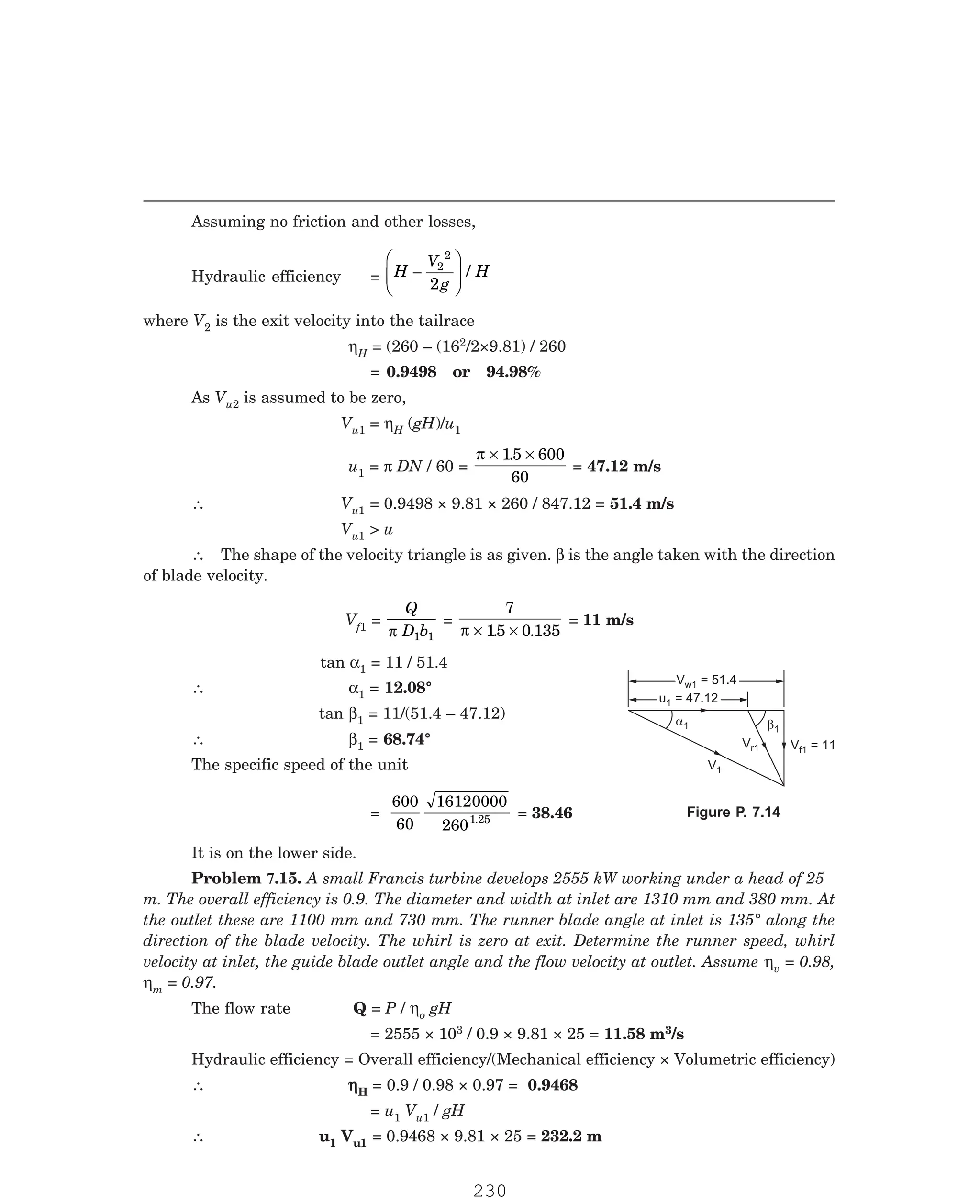
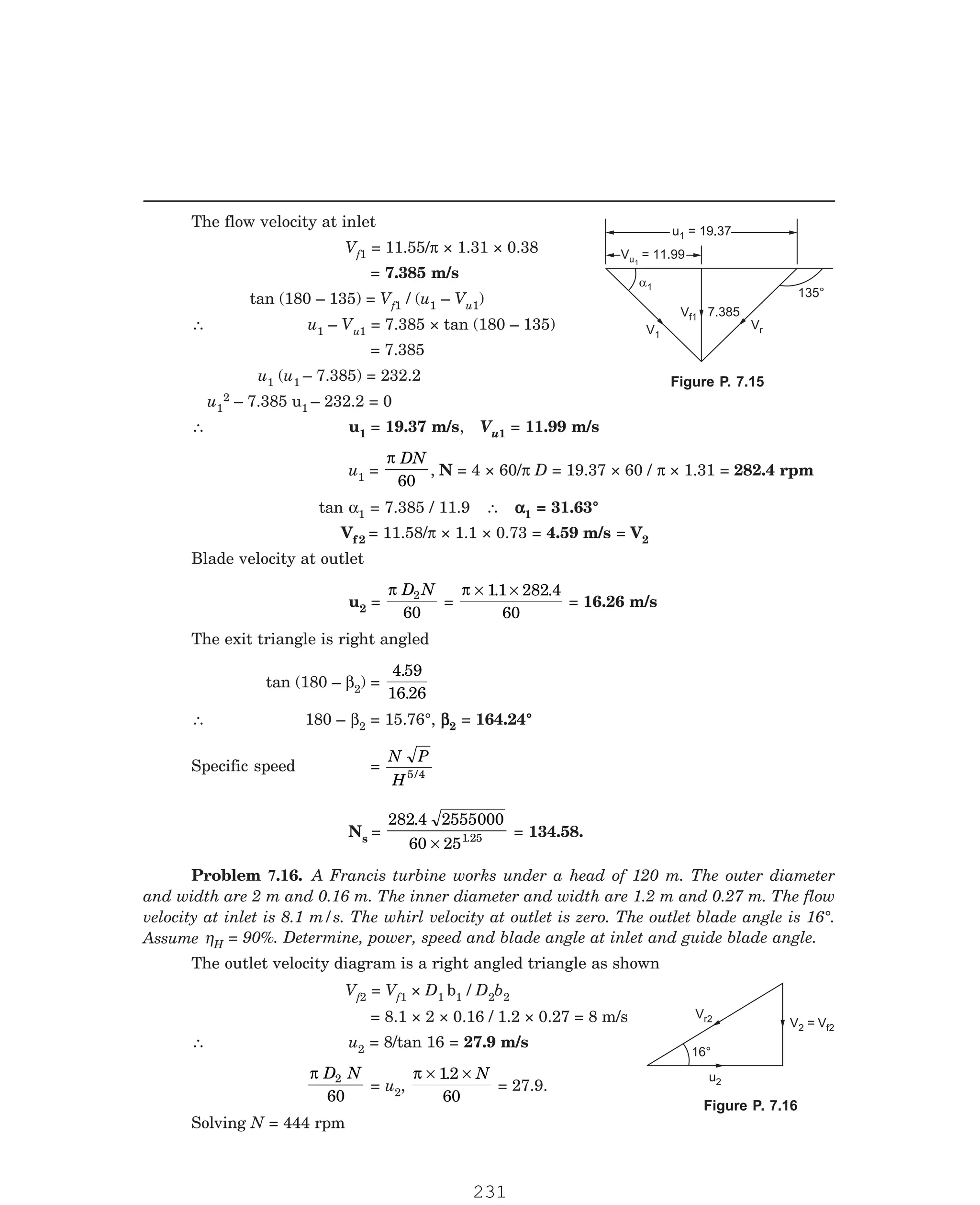
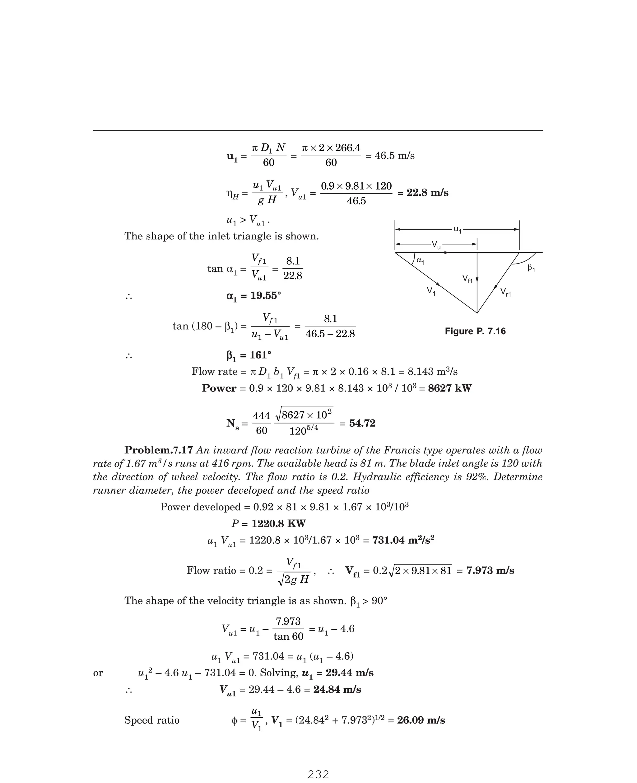
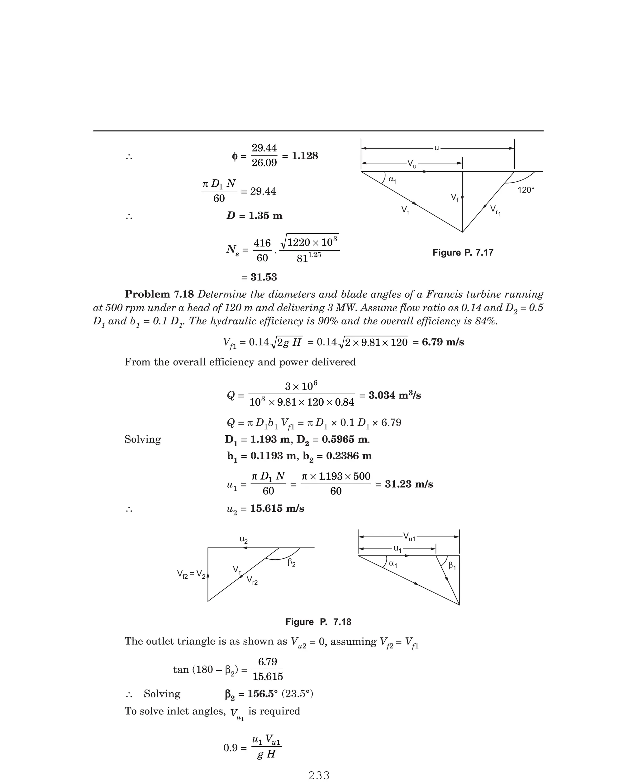
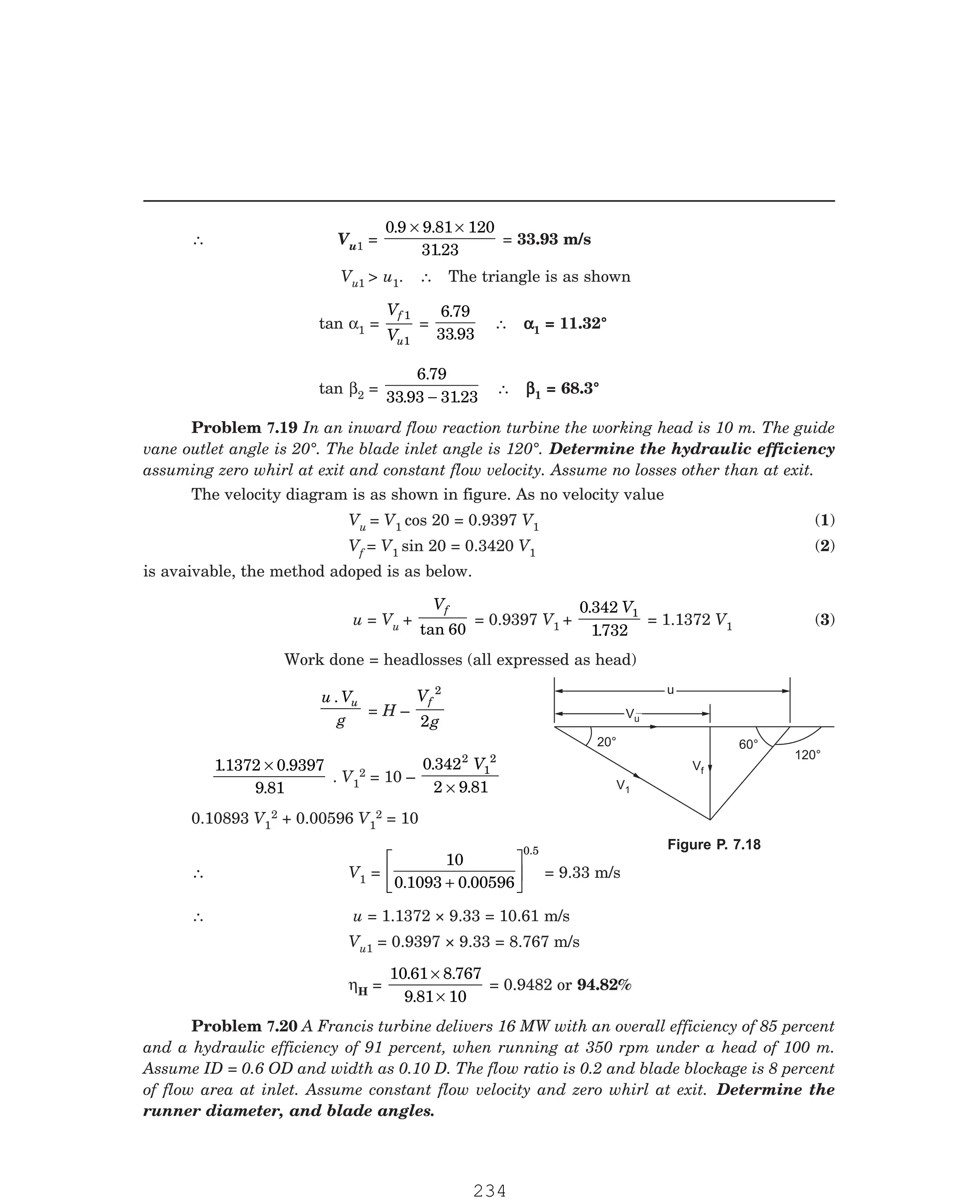
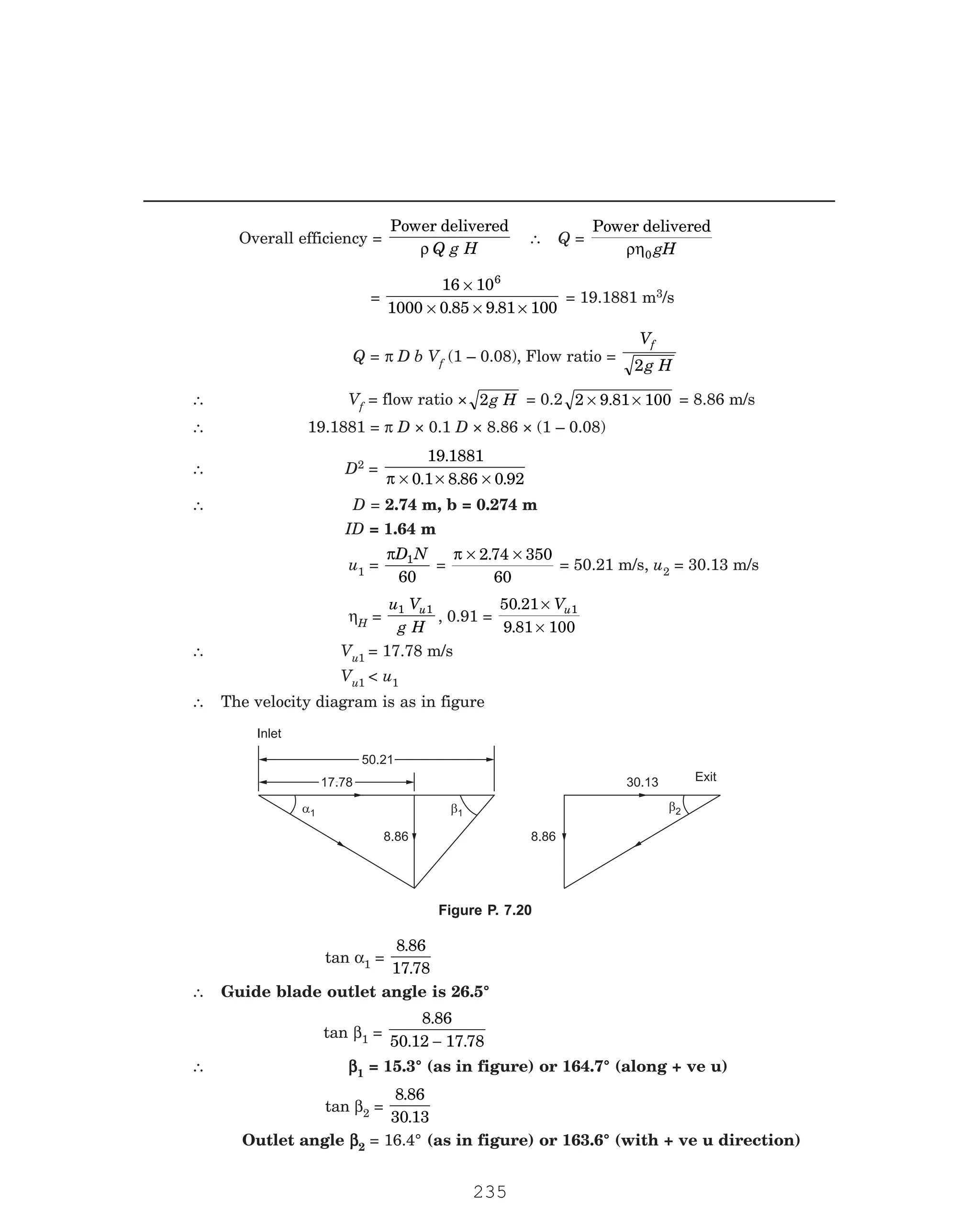
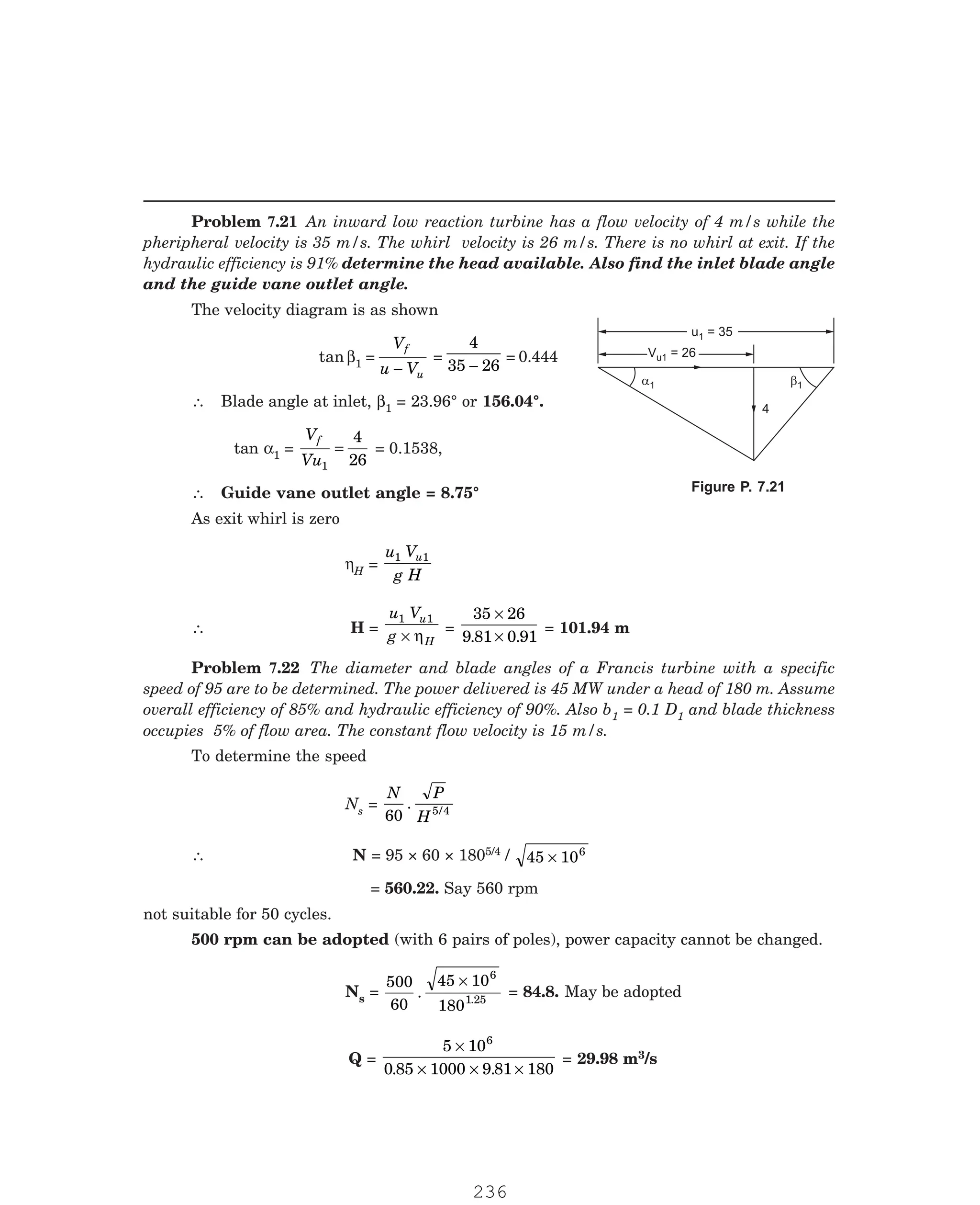
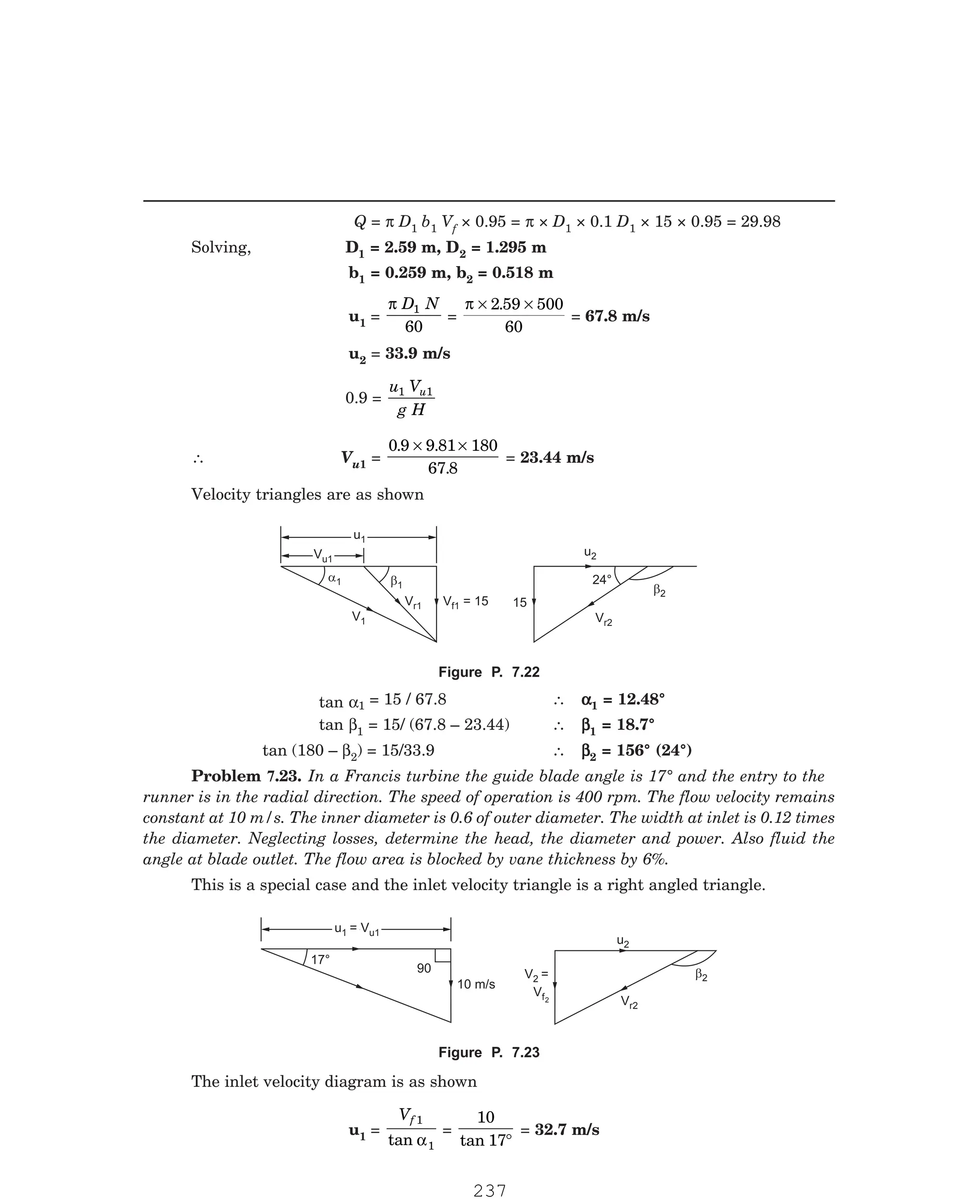
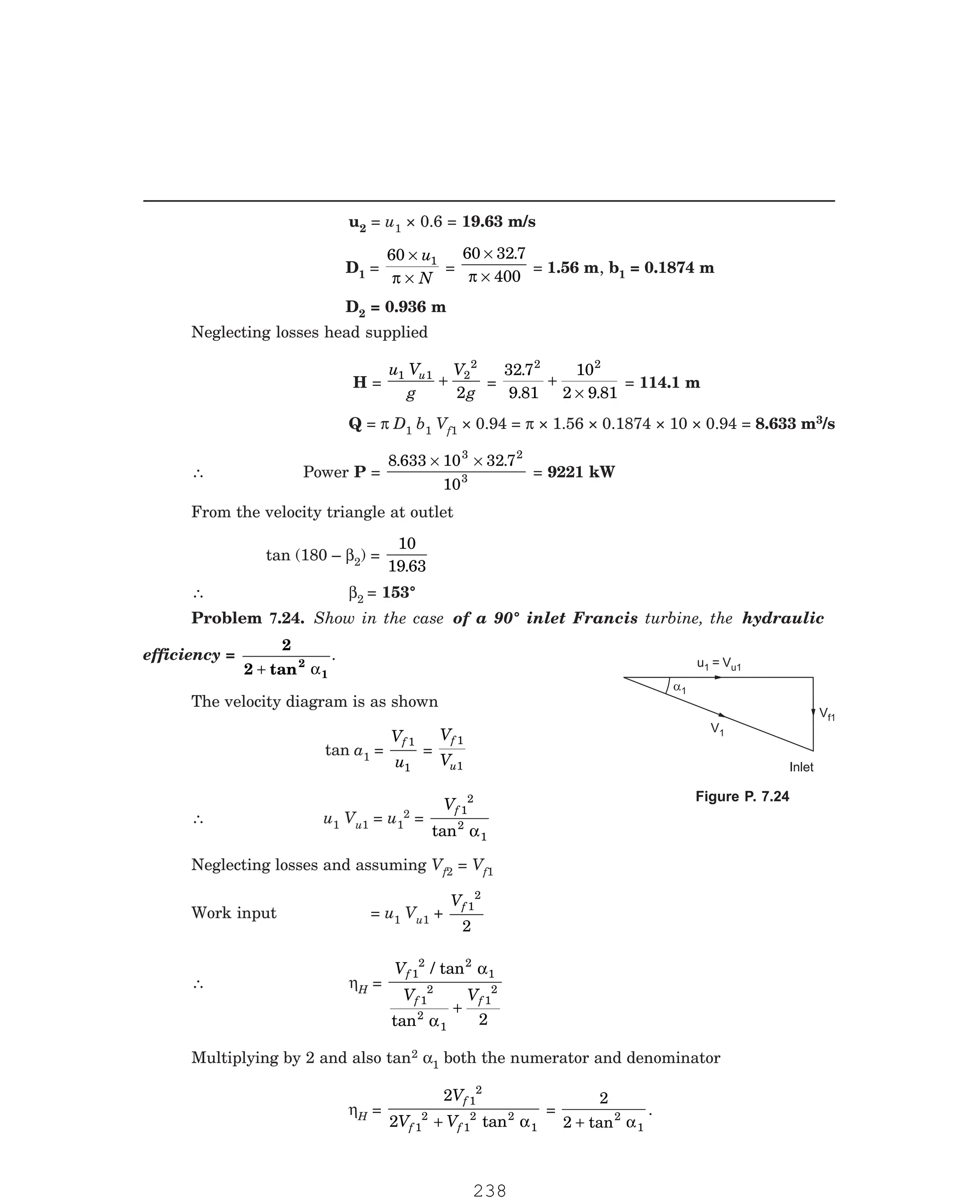
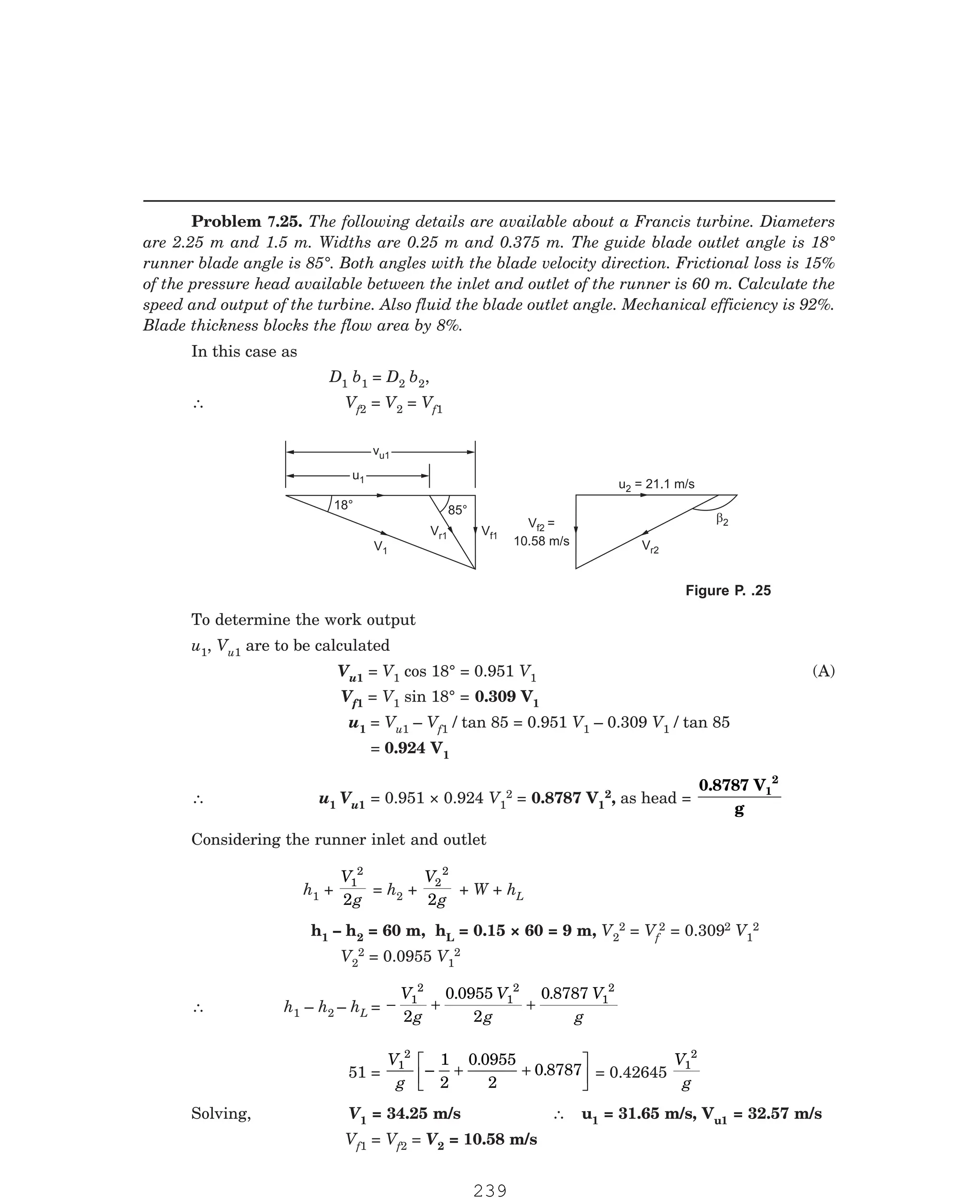
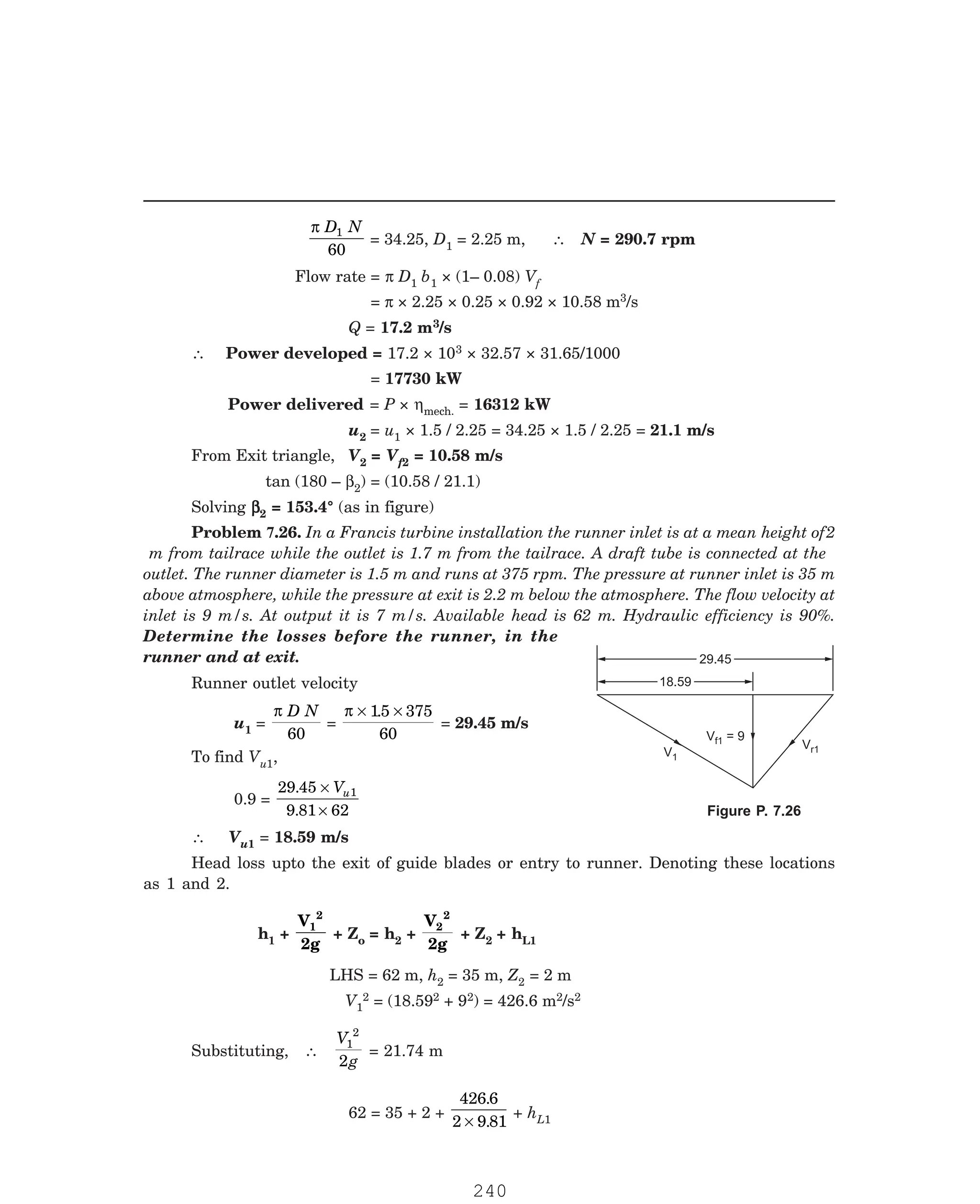
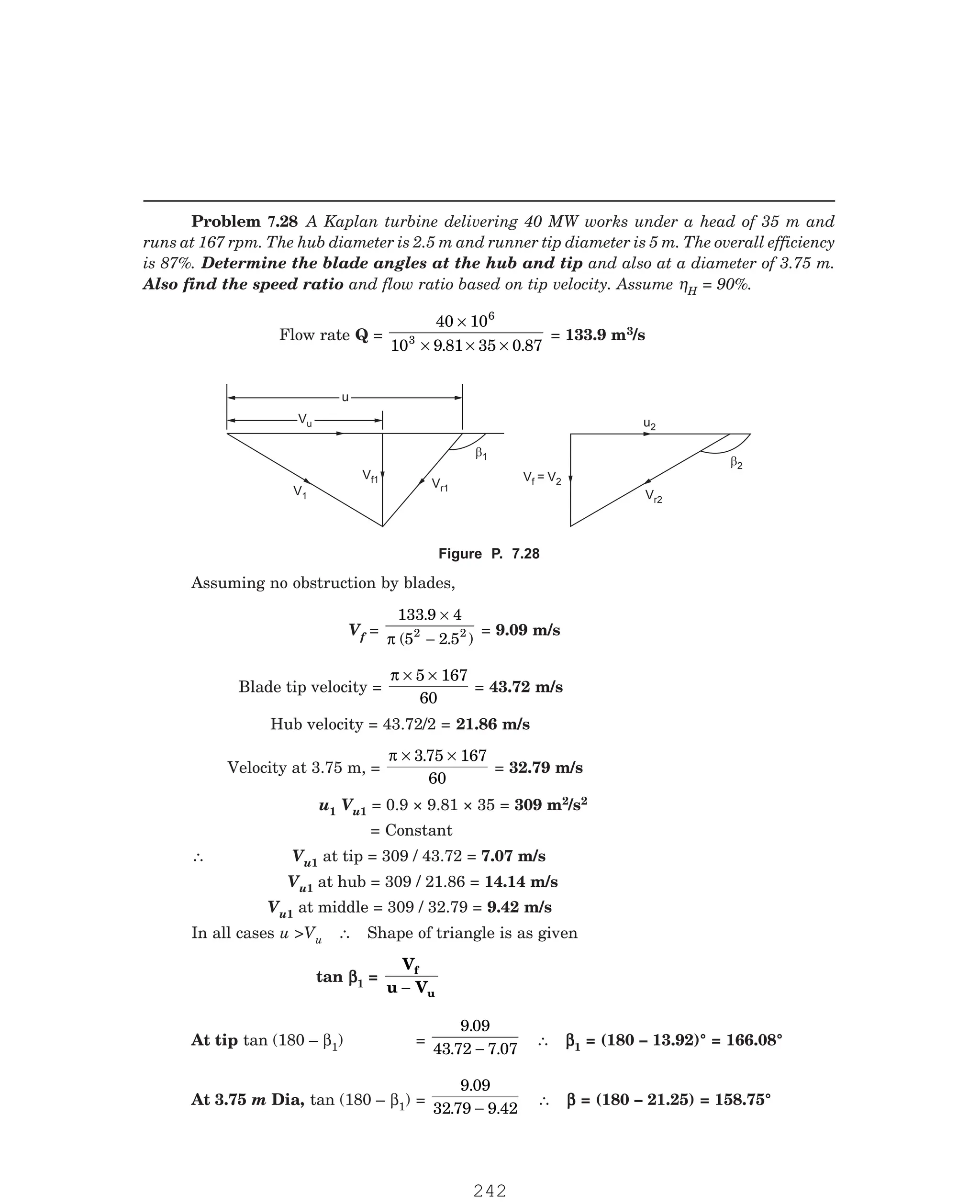
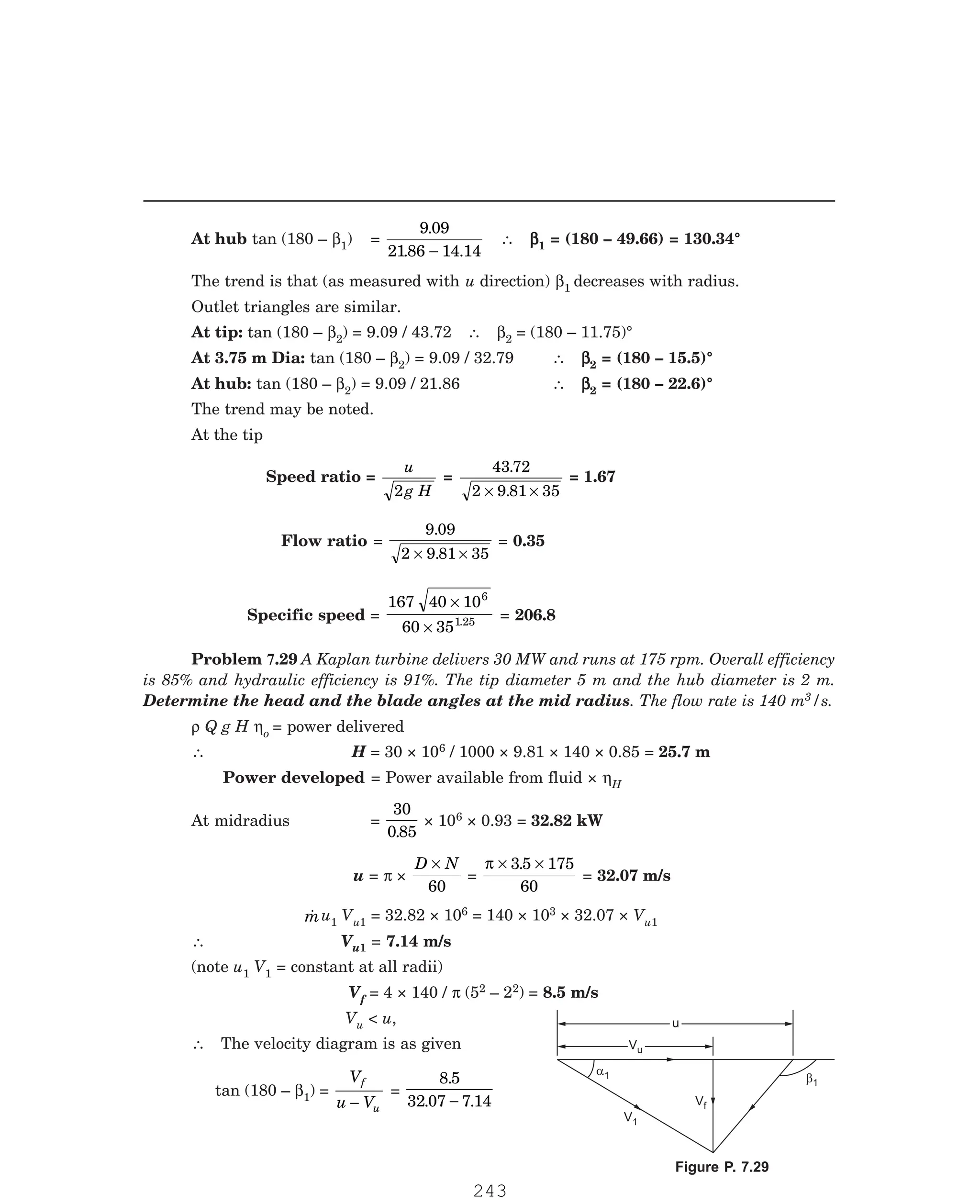
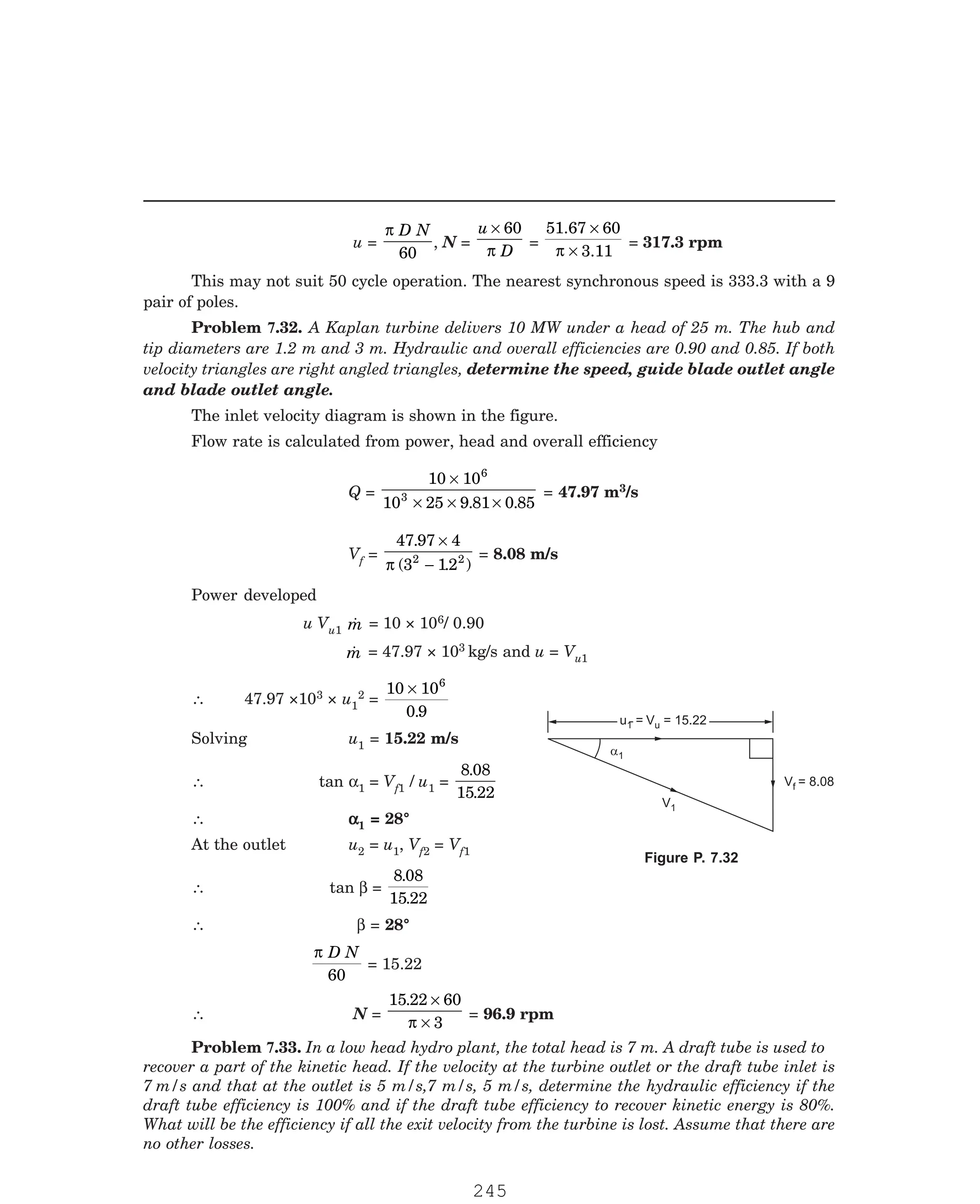


![P-2D:N-fluidFlu14-1.pm5
by the difference in pressure between the turbine entry and tailrace level. The following
efficiencies are generally used.
1. Hydraulic efficiency : It is defined as the ratio of the power produced by the turbine
runner and the power supplied by the water at the turbine inlet.
ηH =
Power produced by the runner
ρ Q g H
where Q is the volume flow rate and H is the net or effective head. Power produced by the
runner is calculated by the Euler turbine equation P = Qρ [u1 Vu1 – u2 Vu2]. This reflects the
runner design effectiveness.
2. Volumetric efficiency : It is possible some water flows out through the clearance
between the runner and casing without passing through the runner.
Volumetric efficiency is defined as the ratio between the volume of water flowing through
the runner and the total volume of water supplied to the turbine. Indicating Q as the volume
flow and ∆Q as the volume of water passing out without flowing through the runner.
ηv =
Q Q
Q
– ∆
To some extent this depends on manufacturing tolerances.
3. Mechanical efficiency : The power produced by the runner is always greater than
the power available at the turbine shaft. This is due to mechanical losses at the bearings,
windage losses and other frictional losses.
ηm =
Power available at the turbine shaft
4. Overall efficiency : This is the ratio of power output at the shaft and power input by
the water at the turbine inlet.
η0 =
Power available at the turbine shaft
ρ QgH
Also the overall efficiency is the product of the other three efficiencies defind
η0 = NH Nm Nv
The fluid velocity at the turbine entry and exit can have three components in the tangential,
axial and radial directions of the rotor. This means that the fluid momentum can have three
components at the entry and exit. This also means that the force exerted on the runner can
have three components. Out of these the tangential force only can cause the rotation of
the runner and produce work. The axial component produces a thrust in the axial direction,
which is taken by suitable thrust bearings. The radial component produces a bending of the
shaft which is taken by the journal bearings.
(7.4.3)
Power produced by the runner
7.5 EULER TURBINE EQUATION
195](https://crownmelresort.com/image.slidesharecdn.com/hydraulicturbines2-251114192057-bc3f4363/75/HYDRAULIC-TURBINES-with-question-and-answer-pdf-10-2048.jpg)

![P-2D:N-fluidFlu14-1.pm5
V1, V2 Absolute velocities at inlet and outlet.
Vr1, Vr2 Relative velocities at inlet and outlet.
u1, u2 Tangential velocities at inlet and outlet.
Vu1, Vu2 Tangential component of absolute velocities at inlet and outlet.
From inlet velocity triangle, (Vu1 = V1 cos α1)
Vr1
2 = V1
2 + u1
2 – 2u1 V1 cos α1
or u1 V1 cos α1 = Vu1 u1 =
V u vr
1
2
1
2
1
2
2
+ −
(A)
From outlet velocity triangle (Vu2 = V2 cos α2)
Vr2
2 = V2
2 + u2
2 – 2 u2 V2 cos α2
or u2 V2 cos α2 = u2 Vu2 = (V2
2 – u2
2 + Vr2
2)/2 (B)
Substituting in Euler equation,
Power per unit flow rate (here the Vu2 is in the opposite to Vu1)
m(u1 Vu1 + u2 Vu2) =
m
1
2
[(V1
2 – V2
2) + (u1
2 – u2
2) + (Vr2
2 – Vr1
2)]
V V
1
2
2
2
2
−
is the dynamic component of work done
u u
1
2
2
2
2
−
is the centrifugal component of work and this will be present only in the
radial flow machines
u V
r r
2
2
1
2
2
−
is the accelerating component and this will be present only in the reaction
turbines.
The first term only will be present in Pelton or impulse turbine of tangential flow
type.
In pure reaction turbines, the last two terms only will be present.
In impulse reaction turbines of radial flow type, all the terms will be present. (Francis
turbines is of this type).
In impulse reaction turbines, the degree of reaction is defined by the ratio of energy
converted in the rotor and total energy converted.
R =
( – ) ( – )
( – ) ( – ) ( – )
u u V V
V V u u V V
r r
r r
1
2
2
2
2
2
1
2
1
2
2
2
1
2
2
2
2
2
1
2
+
+ +
The degree of reaction is considered in detail in the case of steam turbines where speed
reduction is necessary. Hydraulic turbines are generally operate of lower speeds and hence
degree of reaction is not generally considered in the discussion of hydraulic turbines.
197](https://crownmelresort.com/image.slidesharecdn.com/hydraulicturbines2-251114192057-bc3f4363/75/HYDRAULIC-TURBINES-with-question-and-answer-pdf-12-2048.jpg)


![P-2D:N-fluidFlu14-1.pm5
Once the effective head of turbine entry is known V1 is fixed given by V1 = C gH
v 2 . For
various values of u, the power developed and the hydraulic efficiency will be different. In fact
the out let triangle will be different from the one shown it u Vr2 cos β. In this case Vu2 will be
in the same direction as Vu1 and hence the equation (14.6.3) will read as
P =
m (Vu1 – Vu2) u
It is desirable to arrive at the optimum value of u for a given value of V1
V = Vu1
1
u
u
Vr1
Vr1 u b2
a2
Vu2
Vr2
Vu2
u
Vr2
V2
b2
Alternate exit triangle
u V cos b2
r2
Vu2
V2
u
u
V2
u1 = V1, Vu2 = Vr2 cos β2 – u = kVr1 cos β2 – u = k(V1 – u) cos β2 – u
∴ Vu1 + Vu2 = V1 + k V1 cos β2 – u cos β2 – u
= V1 (1 + k cos β2) – u(1 + k cos β2)
= (1 + k cos β2) (V1 + u)
Substituting in equation (14.6.4)
ηH =
2
1
2
u
V
× (1 + k cos β2) (V1
= 2(1 + k cos β2) u
V
u
V
1
2
1
2
–
L
NMM
O
QPP
u
V1
is called speed ratio and denoted as φ.
∴ ηH = 2(1 + k cos β2) [φ – φ2
and equated to zero.
d
d
H
η
φ
= 2(1 + k cos β2) (1 – 2 φ)
∴ φ =
u
V1
=
1
2
or u = 0.5 V1
In practice the value is some what lower at u = 0.46 V1
Substituting equation (14.6.6) in (14.6.4a) we get
ηH = 2(1 + k cos β2) [0.5 – 0.52]
. Equation 7.6.4
can be modified by using the following relations.
Figure 7.6.4 Velocity triangles Pelton turbine
V
+ u) (7.6.4a)
] (7.6.5)
To arrive at the optimum value of φ, this expression is differentiated with respect to φ
201](https://crownmelresort.com/image.slidesharecdn.com/hydraulicturbines2-251114192057-bc3f4363/75/HYDRAULIC-TURBINES-with-question-and-answer-pdf-16-2048.jpg)


![P-2D:N-fluidFlu14-2.pm5
u1 = Vf [cot α1 + cot β1]
∴ u1Vu1 = Vf1
2 cot α1 [cot α1 + cot β1]
Energy supplied to the runner is
u1 Vu1 +
V2
2
2
= u1 Vu1 +
Vf 2
2
2
= u1 Vu1 +
Vf 1
2
2
(Assume Vf2 = Vf1)
∴ ηb=
V
V
V
f
f
f
1
2
1 1 1
1
2
1
2
1 1 1
2
cot [cot cot ]
cot [cot cot ]
α α β
α α β
+
+ +
Multiply by 2 and add and subtract Vf1
2 in the numerator to get
ηb= 1 –
1
1 2 1 1 1
+ +
cot (cot cot )
α α β
In case β
β
β
β
β1 = 90°
ηb= 1 –
1
1
2
2
1
+
tan α
=
2
2 2
1
+ tan α
In this case Vu1 = u1
100
80
60
40
20
0
50
40
30
20
10
0
600
500
400
300
200
100
0
Water
Power
=
Power
Input
(kW)
Value
of
h
(m)
Brake Power = Power output (kW)
0 500
50 100 150 200 250 300 350 400 450
Head
Head
Efficiency
Efficiency
Power input
Power input
n = 600 rpm
n = 600 rpm
The efficiency curve is not as flat as that of impulse turbine. At part loads the efficiency
is relatively low. There is a drop in efficiency after 100% load.
The characteristics of Francis turbine is shown in Figure 7.7.8.
213](https://crownmelresort.com/image.slidesharecdn.com/hydraulicturbines2-251114192057-bc3f4363/75/HYDRAULIC-TURBINES-with-question-and-answer-pdf-28-2048.jpg)


![P-2D:N-fluidFlu14-2.pm5
Cavitation can occur in the case of reaction turbines at the turbine exit or draft tube
inlet where the pressure may be below atmospheric level. In the case of pumps such damage
may occur at the suction side of the pump, where the absolute pressure is generally below
atmospheric level.
In addition to the damage to the runner cavitation results in undesirable vibration noise
and loss of efficiency. The flow will be disturbed from the design conditions. In reaction turbines
the most likely place for cavitation damage is the back sides of the runner blades near their
trailing edge. The critical factor in the installation of reaction turbines is the vertical distance
from the runner to the tailrace level. For high specific speed propeller units it may be desirable
to place the runner at a level lower than the tailrace level.
To compare cavitation characteristics a cavitation parameter known as Thoma cavitation
coefficient, σ, is used. It is defined as
σ =
h h z
h
a r
where ha is the atmospheric head hr is the vapour pressure head, z is the height of the runner
outlet above tail race and h is the total operating head. The minimum value of σ at which
cavitation occurs is defined as critical cavitation factor σe. Knowing σc the maximum value of
z can be obtained as
z = ha – hv – σe
c is found to be a function of specific speed. In the range of specific speeds for Francis
turbine σc varies from 0.1 to 0.64 and in the range of specific speeds for Kaplan turbine σc
varies from 0.4 to 1.5. The minimum pressure at the turbine outlet, h0 can be obtained as
h0 = ha – z – σc
There are a number of correlations available for the value of σc in terms of specific
speed, obtained from experiments by Moody and Zowski. The constants in the equations depends
on the system used to calculate specific speed.
For Francis runners σc = 0.006 + 0.55 (Ns/444.6)1.8
c = 0.1 + 0.3 [Ns/444.6]2.5
Francis runner σc = 0.625
Ns
380 78
2
.
L
NM O
QP
For Kaplan runner σc = 0.308 +
1
6 82 380 78
2
. .
Ns
F
HG I
K
z = Pa – Pv – σc h = 8.6 – 0.17 – 0.3 × 20 = 2.43 m.
The turbine outlet can be set at 2.43 m above the tailrace level.
− −
(7.8.1)
h (7.8.2)σ
H (7.8.3)
(7.8.4)
For Kaplan runners σ (7.8.5)
Other empirical corrlations are
J (7.8.7)
Example 7.9. The total head on a Francis turbine is 20 m. The machine is at an elevation where
the atmosphic pressure is 8.6 m. The pressure corresponding to the water temperature of 15° C is
0.17 m. It critical cavitation factor is 0.3, determine the level of the turbine outlet above the tail race.
217](https://crownmelresort.com/image.slidesharecdn.com/hydraulicturbines2-251114192057-bc3f4363/75/HYDRAULIC-TURBINES-with-question-and-answer-pdf-32-2048.jpg)


![P-2D:N-fluidFlu14-3.pm5
Jet diameter is found from flow rate and jet velocity.
πd2
4
× Vj = Q, d =
6 0372 4
76 43
0.5
.
.
×
×
L
NM O
QP
π
= 0.3171 m
Jet speed ratio is
D
d
= 12, ∴ D = 12 × 0.3171 = 3.8 m
The turbine rotor speed is determined from the tangential velocity
π DN
60
= u,
N =
u
D
× 60
π
= 35.16 × 60 / π × 3.8 = 176.71 rpm
Ns =
176.61
60
.
15 10
310
6
5/4
×
= 8.764
is 0.2096
d
D
, φ = 0.48, ηo = 90%, Cv = 0.98
Ns =
N P
gH
ρ1/2 5 4
( ) /
, where N is rps.
Q =
π d2
4
× Vj =
π d2
4
× 0.98 [2g H]1/2
= 3.4093 d2 H1/2
P = ηo × ρ g Q H = 0.9 × 1000 × 9.81 × 3.4093 d2 H1/2 × H
= 30100.73 d2 H1.5
N =
u
d
π
, u = 0.48 Vj = 0.48 × 0.98 2g H1/2 = 2.0836 H1/2
∴ N = 0.6632 H1/2 D – 1
∴ Ns =
0 6632 1/2
. H
D
[30100.73 d2H1.5]1/2 / 10001/2 g1.25 H1.25
= 115 068
1
.
.25
dH
D
/ 549 H1.25 = 0.2096
d
D
3/s. Total head is 115 m. For shockless
entry determine the angle of the inlet guide vane. Also find the absolute velocity at entrance, the
Problem 7.12. Show that for the following constants, the dimensionless specific speed
Problem 7.13. The outer diameter of a Francis runner is 1.4 m. The flow velocity at
inlet is 9.5 m/s. The absolute velocity at the exit is 7 m/s. The speed of operation is 430 rpm.
The power developed is 12.25 MW, with a flow rate of 12 m
228](https://crownmelresort.com/image.slidesharecdn.com/hydraulicturbines2-251114192057-bc3f4363/75/HYDRAULIC-TURBINES-with-question-and-answer-pdf-43-2048.jpg)
![P-2D:N-fluidFlu14-3.pm5
runner blade angle at inlet and the loss of head in the unit. Assume zero whirl at exit. Also fluid
the specific speed.
The runner speed u1 =
π D N
60
=
π × ×
430 14
60
.
= 31.52 m/s
As Vu2 = 0,
Power developed =
m Vu1 u1
12.25 × 106 = 12 × 103 × Vu1 × 31.52
Solving Vu1 = 32.39 m/s
Vu1 u1
∴ The shape of the inlet
Velocity triangle is as given. Guide blade angle αr
tan α1 =
9 5
32 39
.
.
∴ α
α
α
α
α1 = 16.35°
V1 = (Vf1
2 + Vu1
2)0.5 = [9.52 + 32.392]0.5 = 33.75 m/s
Blade inlet angle β1
tan β1 = 9.5 / (32.39 – 31.52)
∴ β
β
β
β
β1 = 84.77°
Total head = 115 m. head equal for Euler work =
m Vu1 u1/g
=
32 39 3152
9 81
. .
.
×
= 104.07 m
Head loss in the absolute velocity at exit
=
7
2 9 81
2
× .
= 2.5 m
∴ Loss of head = 115 – 104.07 – 2.5 = 8.43 m
Ns =
430
60
12 25 10
115
6
1
.
.
.25
×
= 223.12
As the inner diameter is not known blade angle at outlet cannot be determined.
3/s . The exit velocity at the draft tube outlet is 16 m/s. Assuming zero whirl velocity at exit
and neglecting blade thickness determine the overall and hydraulic efficiency and rotor blade
angle at inlet. Also find the guide vane outlet angle :
Overall efficiency =
Power developed
Hydraulic power
=
16120 10
7 1000 9 81 260
3
×
× × ×
.
ηo = 0.9029 or 90.29%
V = 32.39 m/s
u1
V = 32.39 m/s
u1
u = 31.51
1
u = 31.51
1
a1 b1
V = 9.5 m/s
f1
Figure P. 7.13
Problem 7.14. A Francis turbine developing 16120 kW under an a head of 260 m runs
at 600 rpm. The runner outside diameter is 1500 mm and the width is 135 mm. The flow rate is
7 m
229](https://crownmelresort.com/image.slidesharecdn.com/hydraulicturbines2-251114192057-bc3f4363/75/HYDRAULIC-TURBINES-with-question-and-answer-pdf-44-2048.jpg)


