Graphs
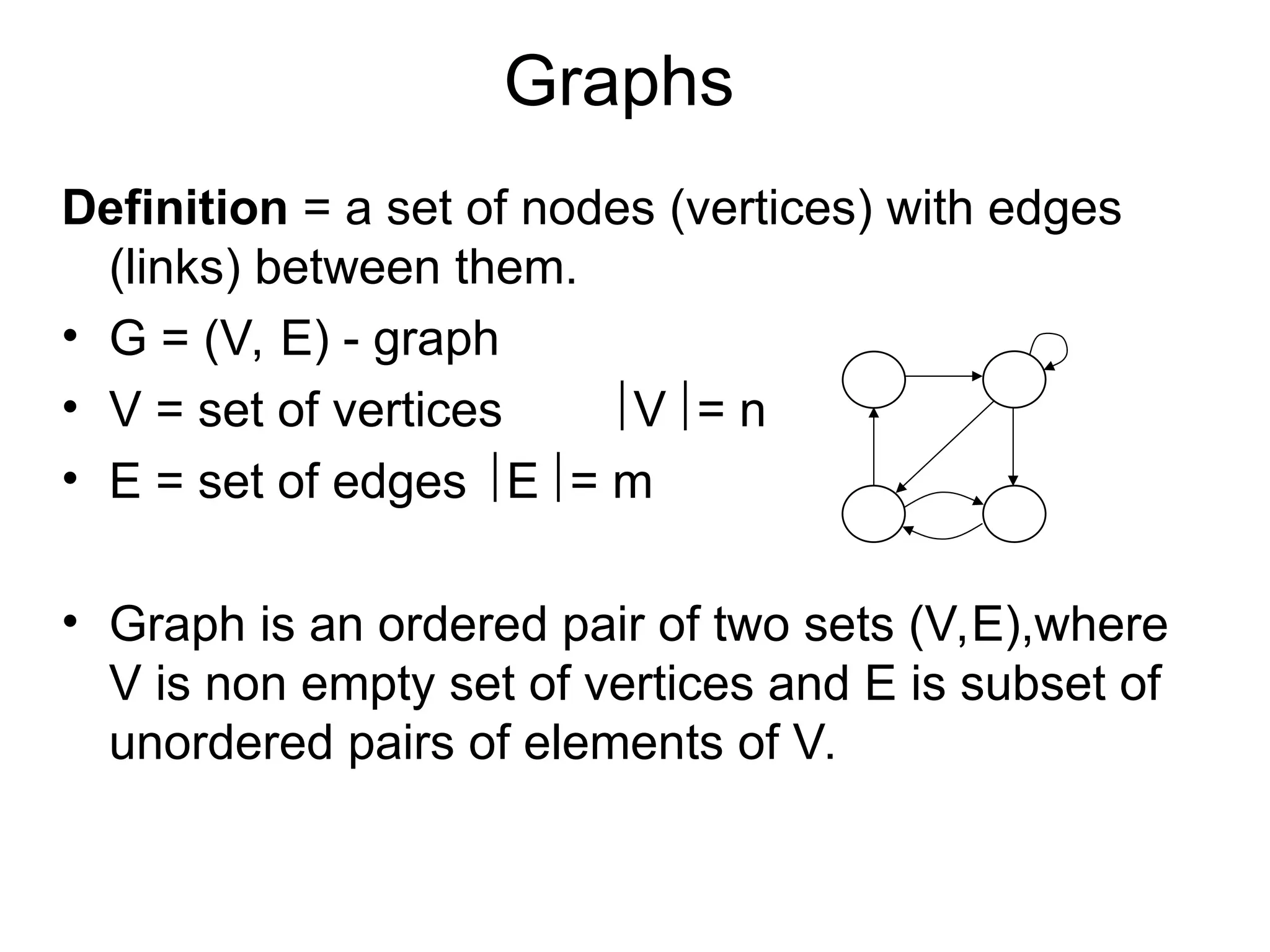
Definition = aset of nodes (vertices) with edges
(links) between them.
• G = (V, E) - graph
• V = set of vertices V = n
• E = set of edges E = m
• Graph is an ordered pair of two sets (V,E),where
V is non empty set of vertices and E is subset of
unordered pairs of elements of V.
1 2
3 4
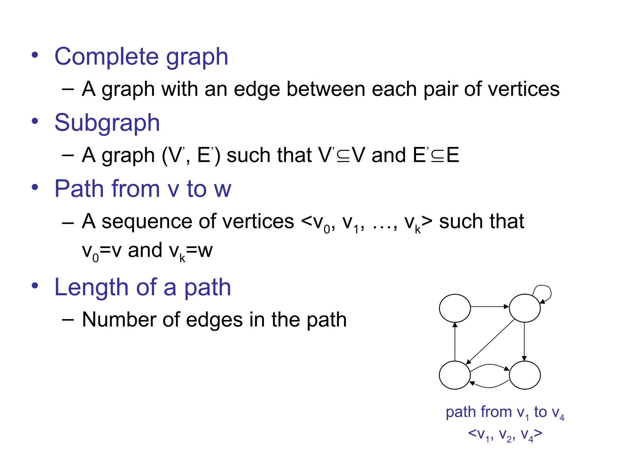
• Complete graph
–A graph with an edge between each pair of vertices
• Subgraph
– A graph (V’
, E’
) such that V’
V and E’
E
• Path from v to w
– A sequence of vertices <v0, v1, …, vk> such that
v0=v and vk=w
• Length of a path
– Number of edges in the path
1 2
3 4
path from v1 to v4
<v1, v2, v4>
5.
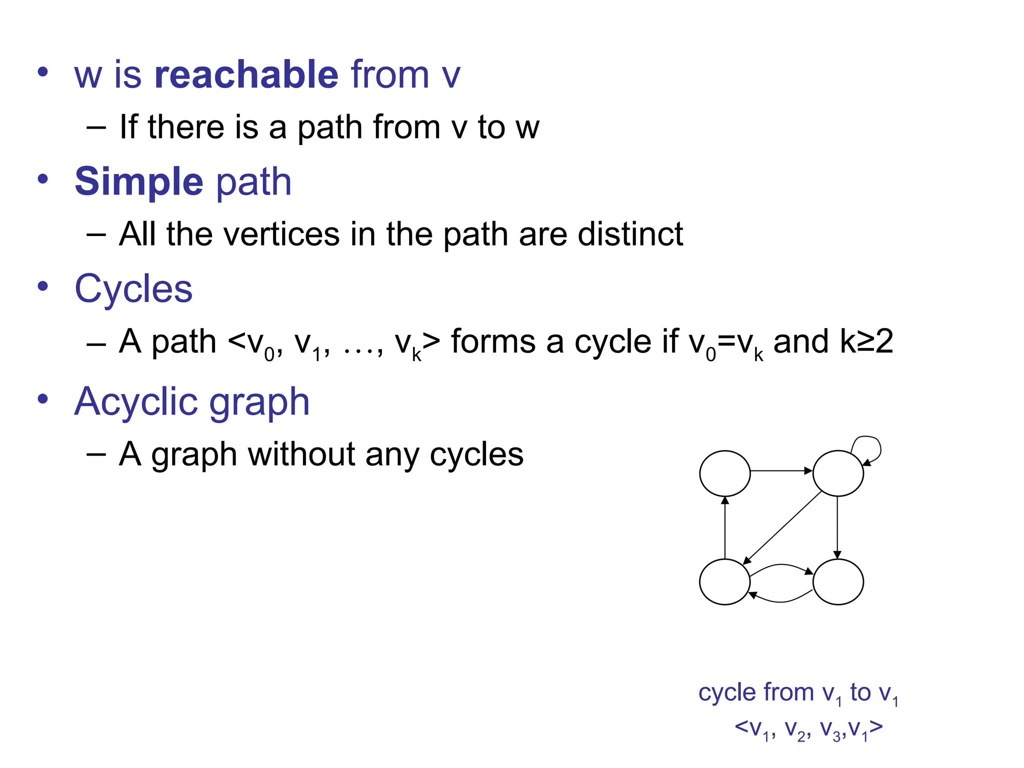
• w isreachable from v
– If there is a path from v to w
• Simple path
– All the vertices in the path are distinct
• Cycles
– A path <v0, v1, …, vk> forms a cycle if v0=vk and k≥2
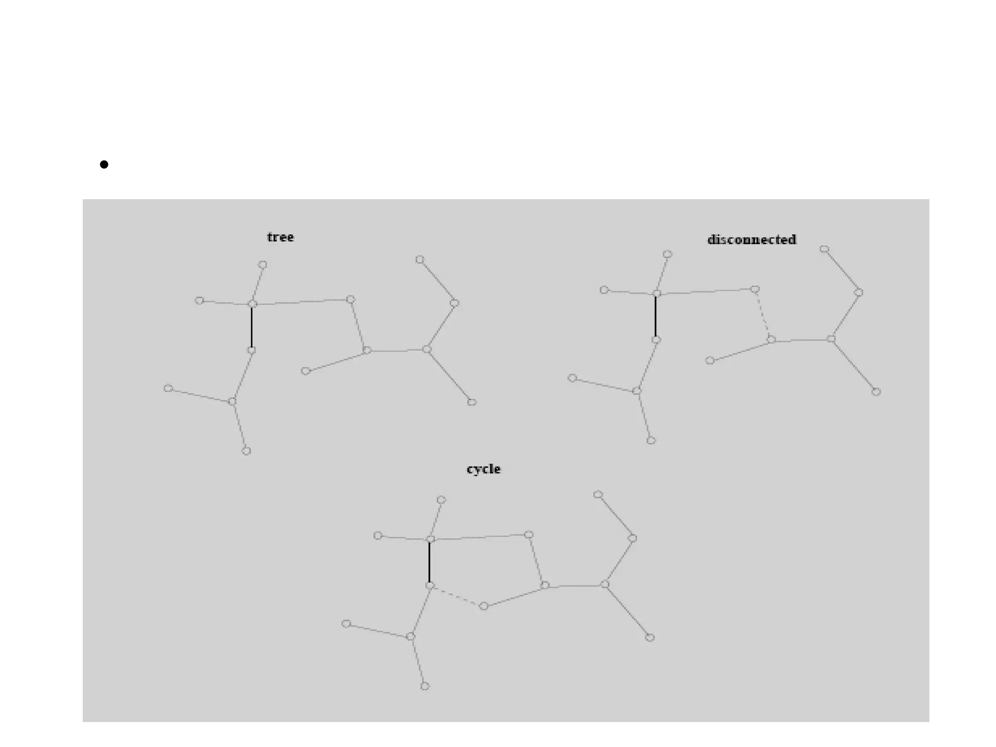
• Acyclic graph
– A graph without any cycles
1 2
3 4
cycle from v1 to v1
<v1, v2, v3,v1>
6.
6
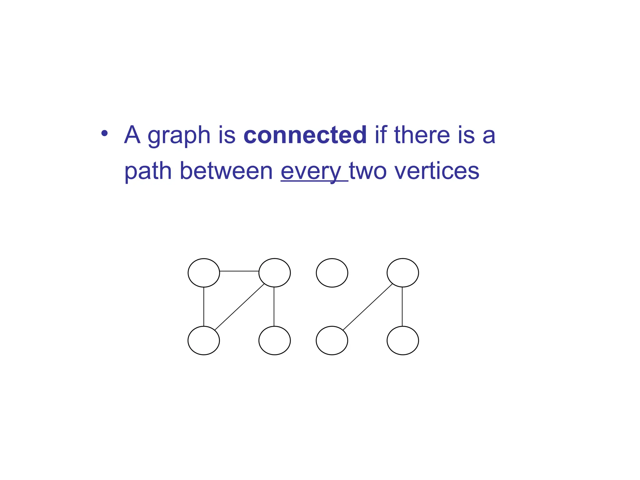
• A graphis connected if there is a
path between every two vertices
1 2
3 4
Connected
1 2
3 4
Not connected
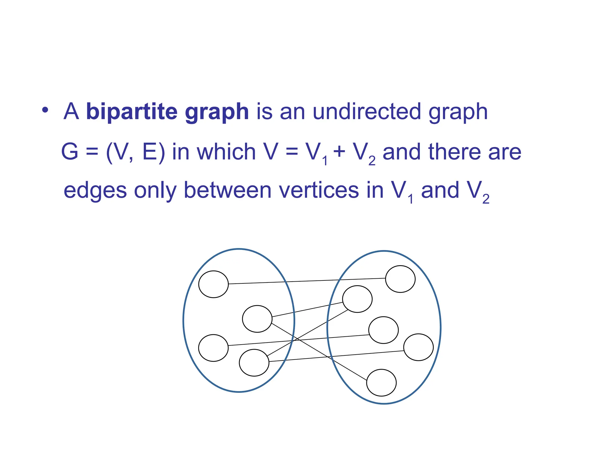
• A bipartitegraph is an undirected graph
G = (V, E) in which V = V1 + V2 and there are
edges only between vertices in V1 and V2
1 2
3
4
4
9
7
6
8
V1 V2
9.
Graph Representation
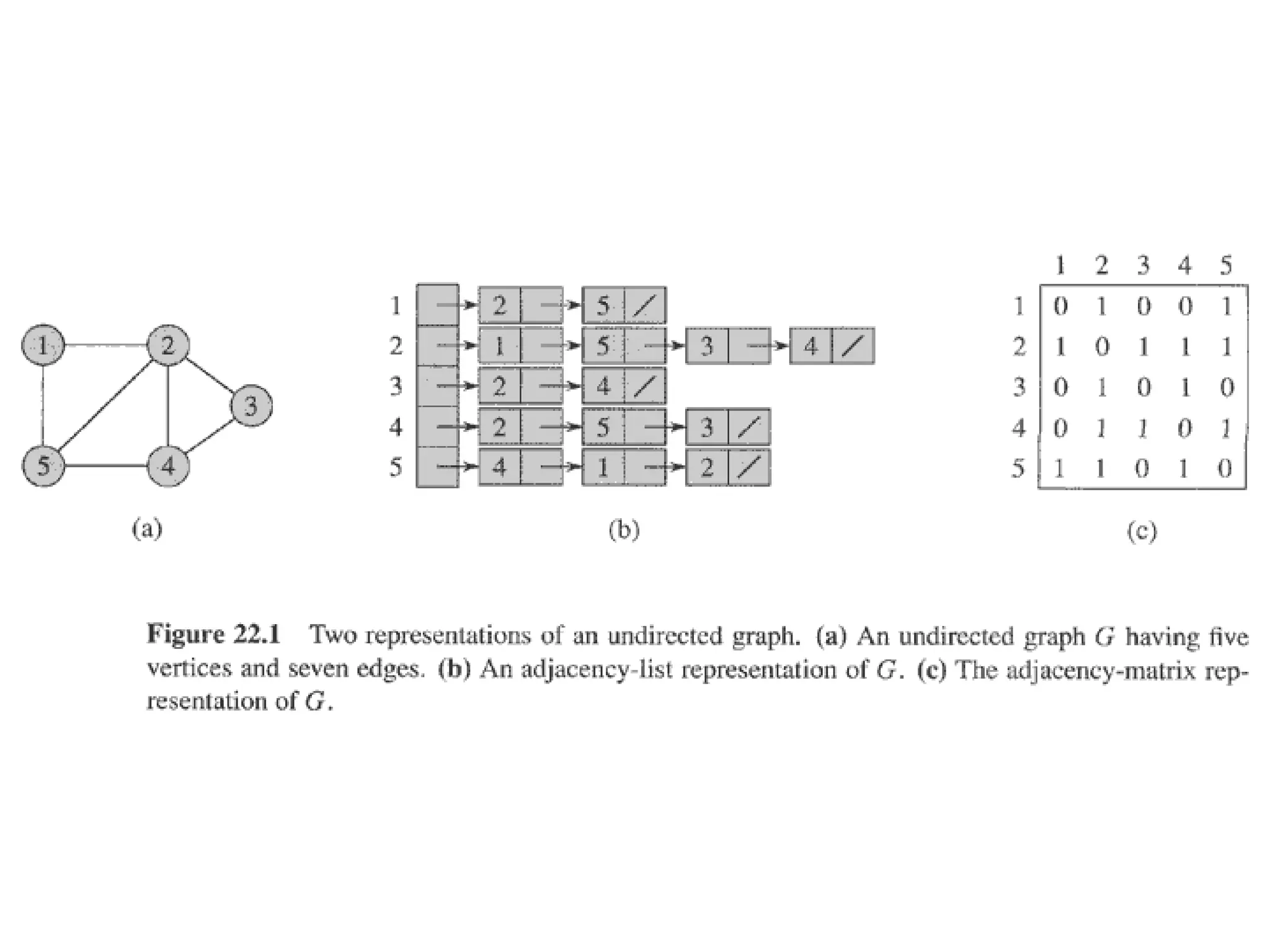
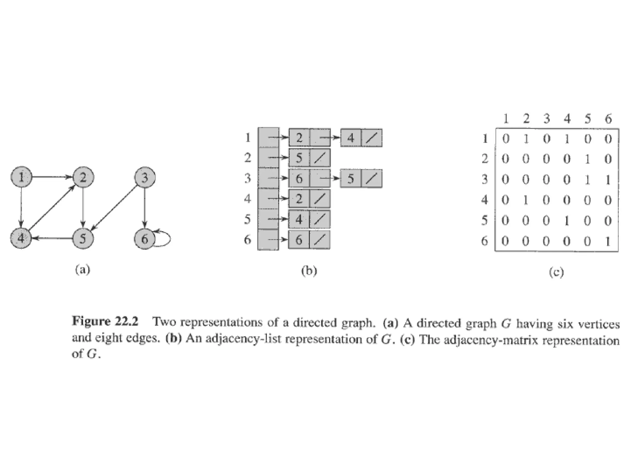
• Adjacencylist representation of G = (V, E)
– An array of V lists, one for each vertex in V
– Each list Adj[u] contains all the vertices v such that
there is an edge between u and v
• Adj[u] contains the vertices adjacent to u (in arbitrary order)
– Can be used for both directed and undirected graphs
1 2
5 4
3
2 5 /
1 5 3 4 /
1
2
3
4
5
2 4
2 5 3 /
4 1 2
Undirected graph
10.
Properties of Adjacency-List
Representation
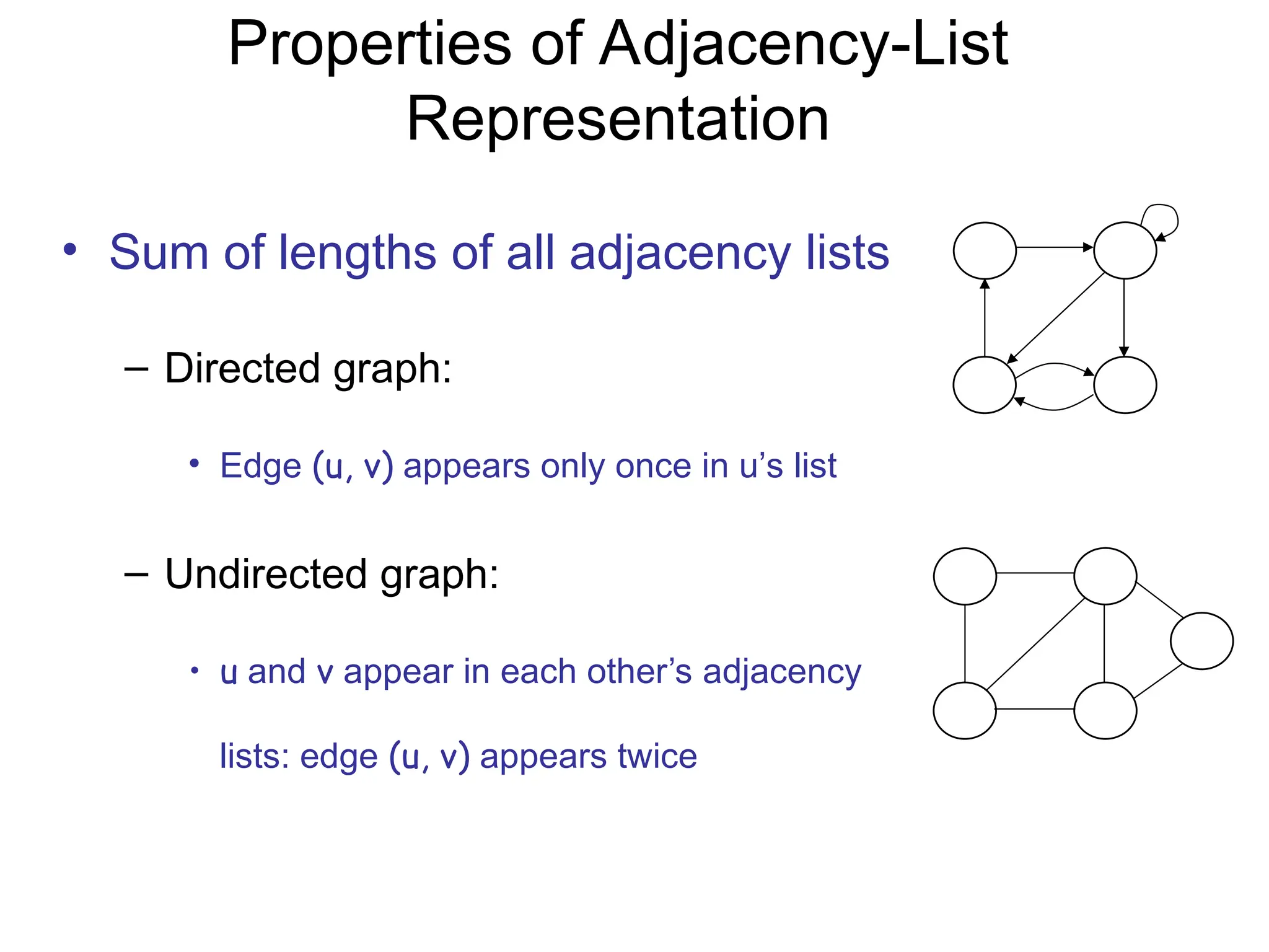
•Sum of lengths of all adjacency lists
– Directed graph:
• Edge (u, v) appears only once in u’s list
– Undirected graph:
• u and v appear in each other’s adjacency
lists: edge (u, v) appears twice
1 2
5 4
3
Undirected graph
1 2
3 4
Directed graph
E
2 E
11.
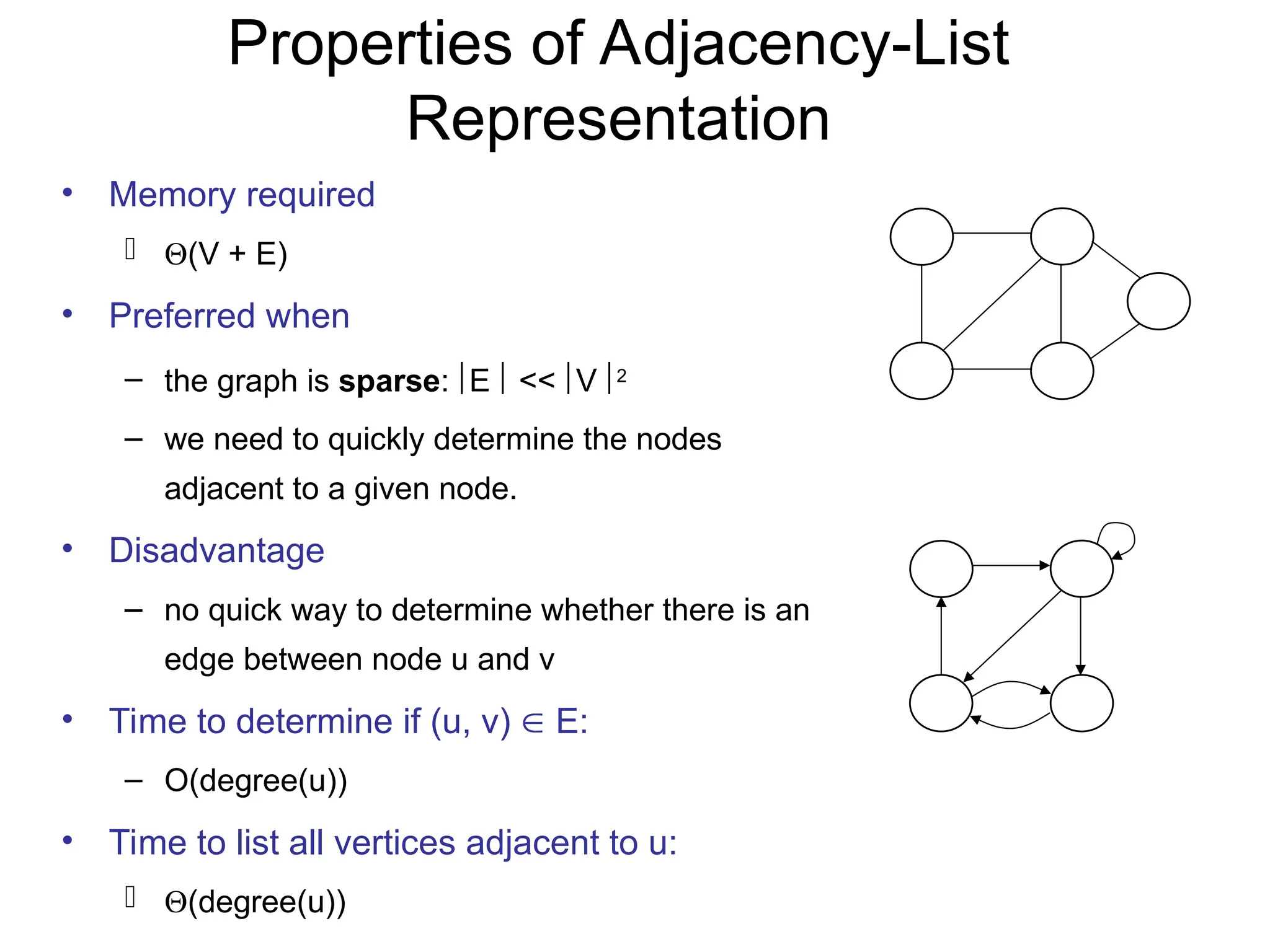
Properties of Adjacency-List
Representation
•Memory required
(V + E)
• Preferred when
– the graph is sparse: E << V 2
– we need to quickly determine the nodes
adjacent to a given node.
• Disadvantage
– no quick way to determine whether there is an
edge between node u and v
• Time to determine if (u, v) E:
– O(degree(u))
• Time to list all vertices adjacent to u:
(degree(u))
1 2
5 4
3
Undirected graph
1 2
3 4
Directed graph
12.
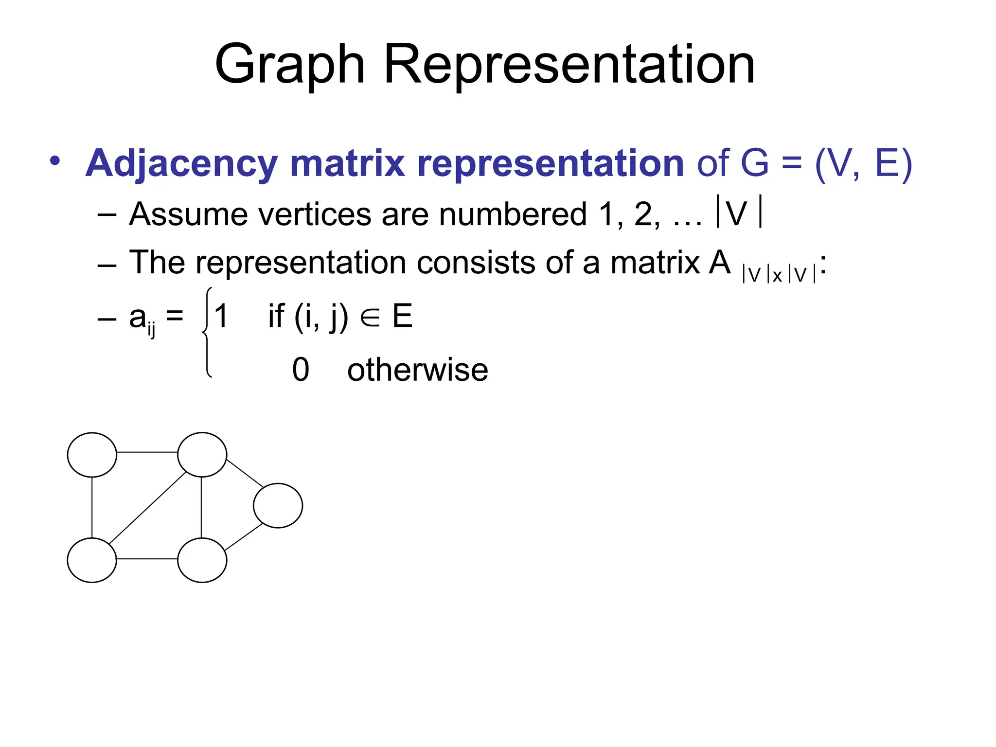
Graph Representation
• Adjacencymatrix representation of G = (V, E)
– Assume vertices are numbered 1, 2, … V
– The representation consists of a matrix A V x V :
– aij = 1 if (i, j) E
0 otherwise
1 2
5 4
3
Undirected graph
1
2
3
4
5
1 2 3 4 5
0 1 1
0 0
1 1 1 1
0
1 1
0 0 0
1 1 1
0 0
1 1 1
0 0
For undirected
graphs, matrix A
is symmetric:
aij = aji
A = AT
13.
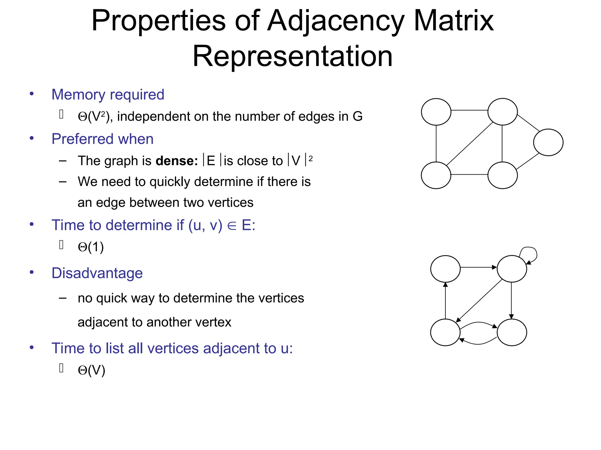
Properties of AdjacencyMatrix
Representation
• Memory required
(V2
), independent on the number of edges in G
• Preferred when
– The graph is dense: E is close to V 2
– We need to quickly determine if there is
an edge between two vertices
• Time to determine if (u, v) E:
(1)
• Disadvantage
– no quick way to determine the vertices
adjacent to another vertex
• Time to list all vertices adjacent to u:
(V)
1 2
5 4
3
Undirected graph
1 2
3 4
Directed graph
14.
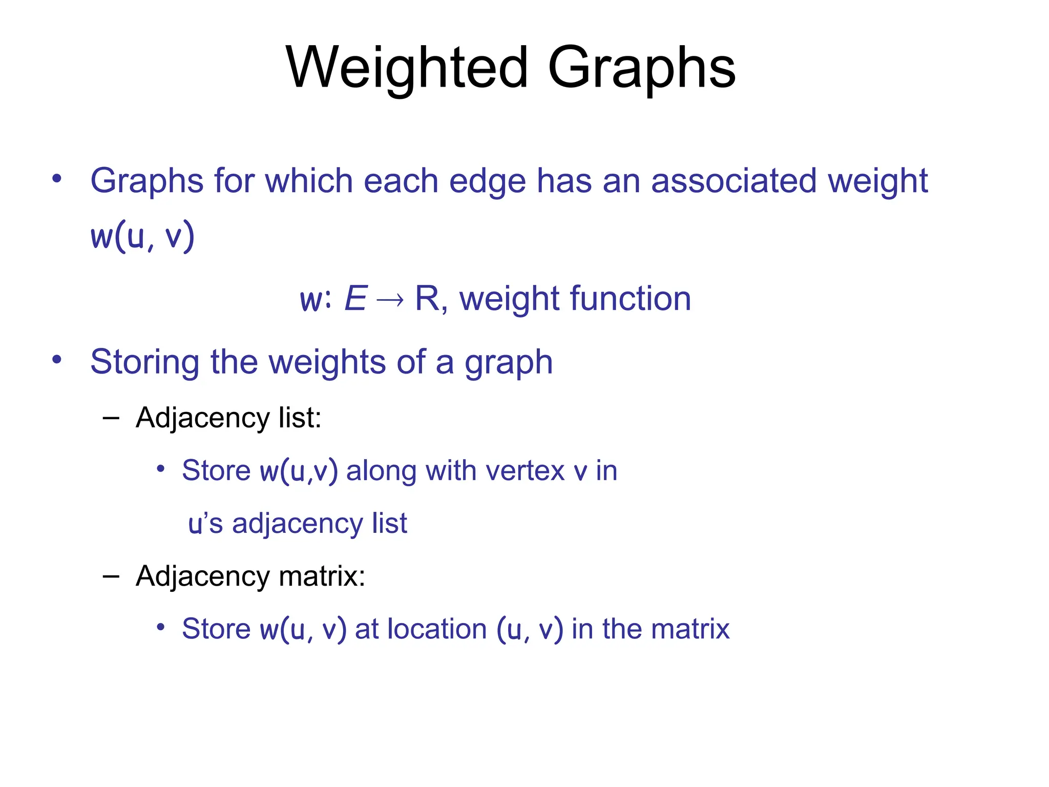
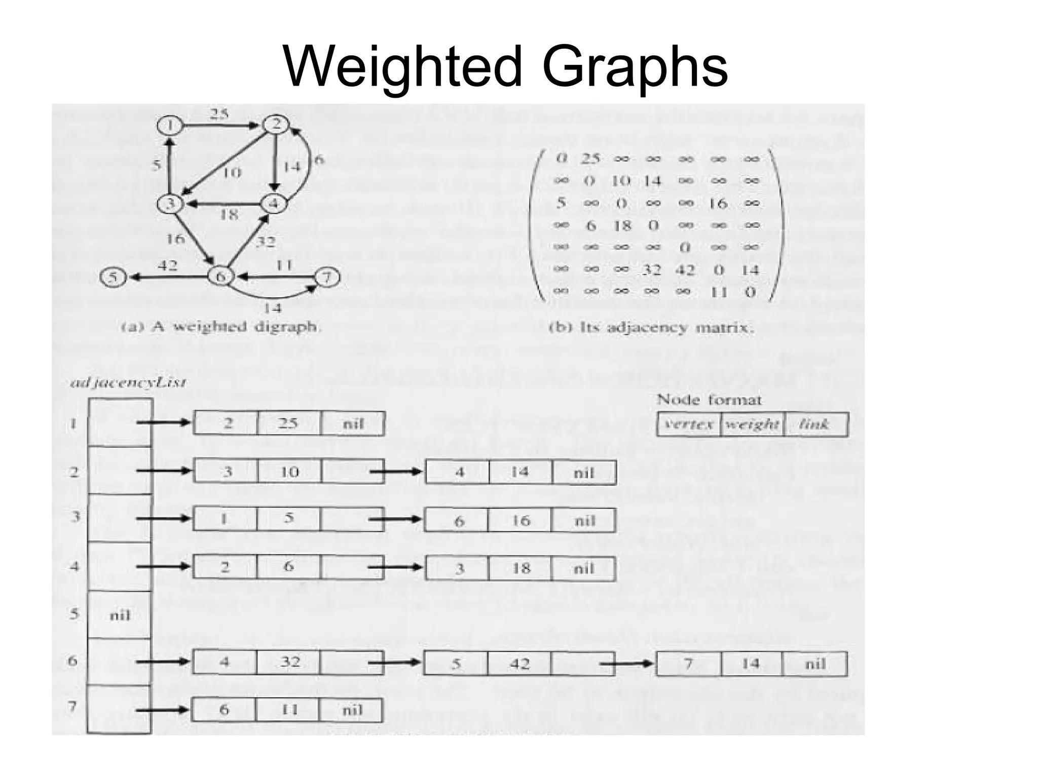
Weighted Graphs
• Graphsfor which each edge has an associated weight
w(u, v)
w: E R, weight function
• Storing the weights of a graph
– Adjacency list:
• Store w(u,v) along with vertex v in
u’s adjacency list
– Adjacency matrix:
• Store w(u, v) at location (u, v) in the matrix
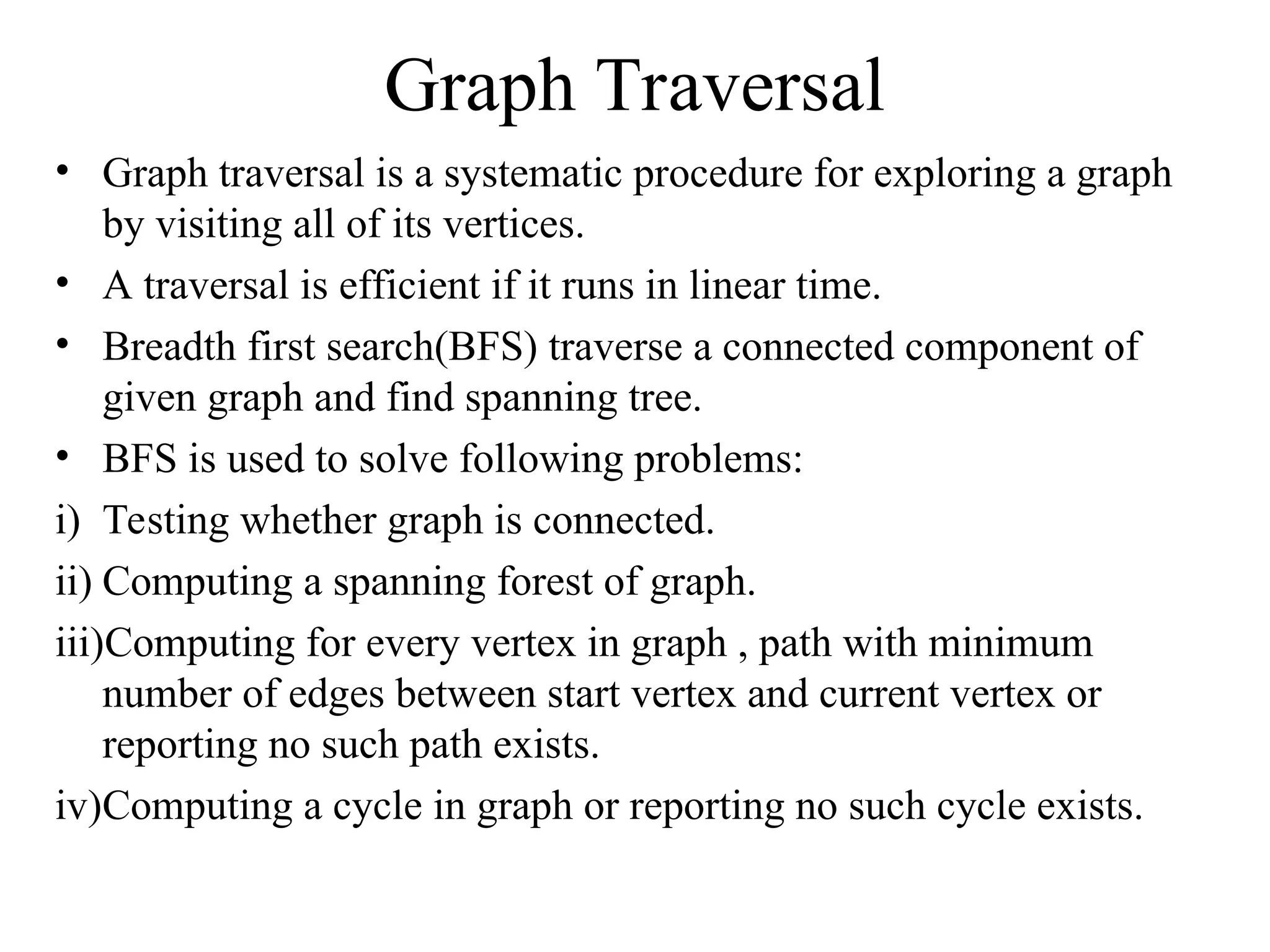
Graph Traversal
• Graphtraversal is a systematic procedure for exploring a graph
by visiting all of its vertices.
• A traversal is efficient if it runs in linear time.
• Breadth first search(BFS) traverse a connected component of
given graph and find spanning tree.
• BFS is used to solve following problems:
i) Testing whether graph is connected.
ii) Computing a spanning forest of graph.
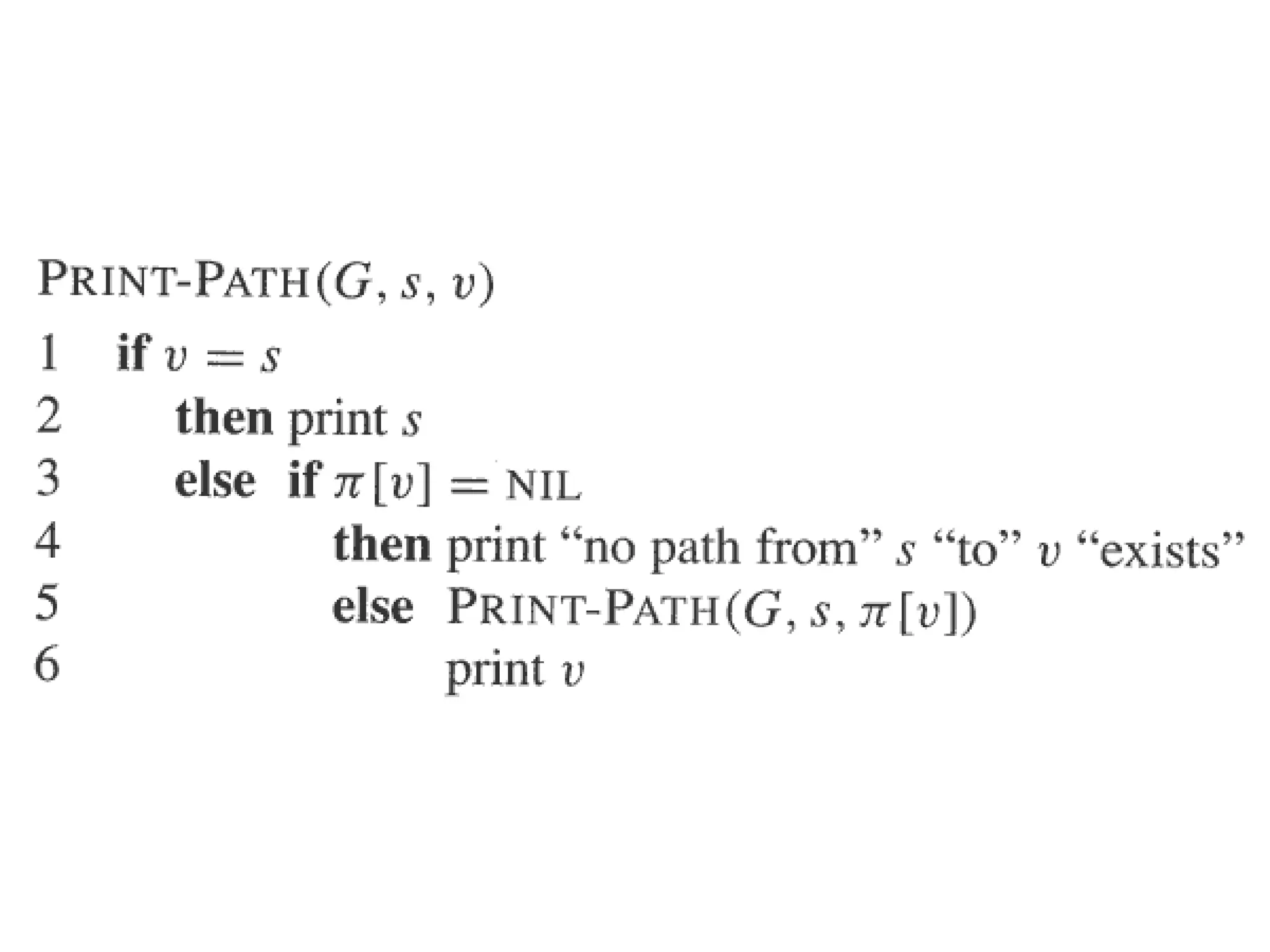
iii)Computing for every vertex in graph , path with minimum
number of edges between start vertex and current vertex or
reporting no such path exists.
iv)Computing a cycle in graph or reporting no such cycle exists.
19.
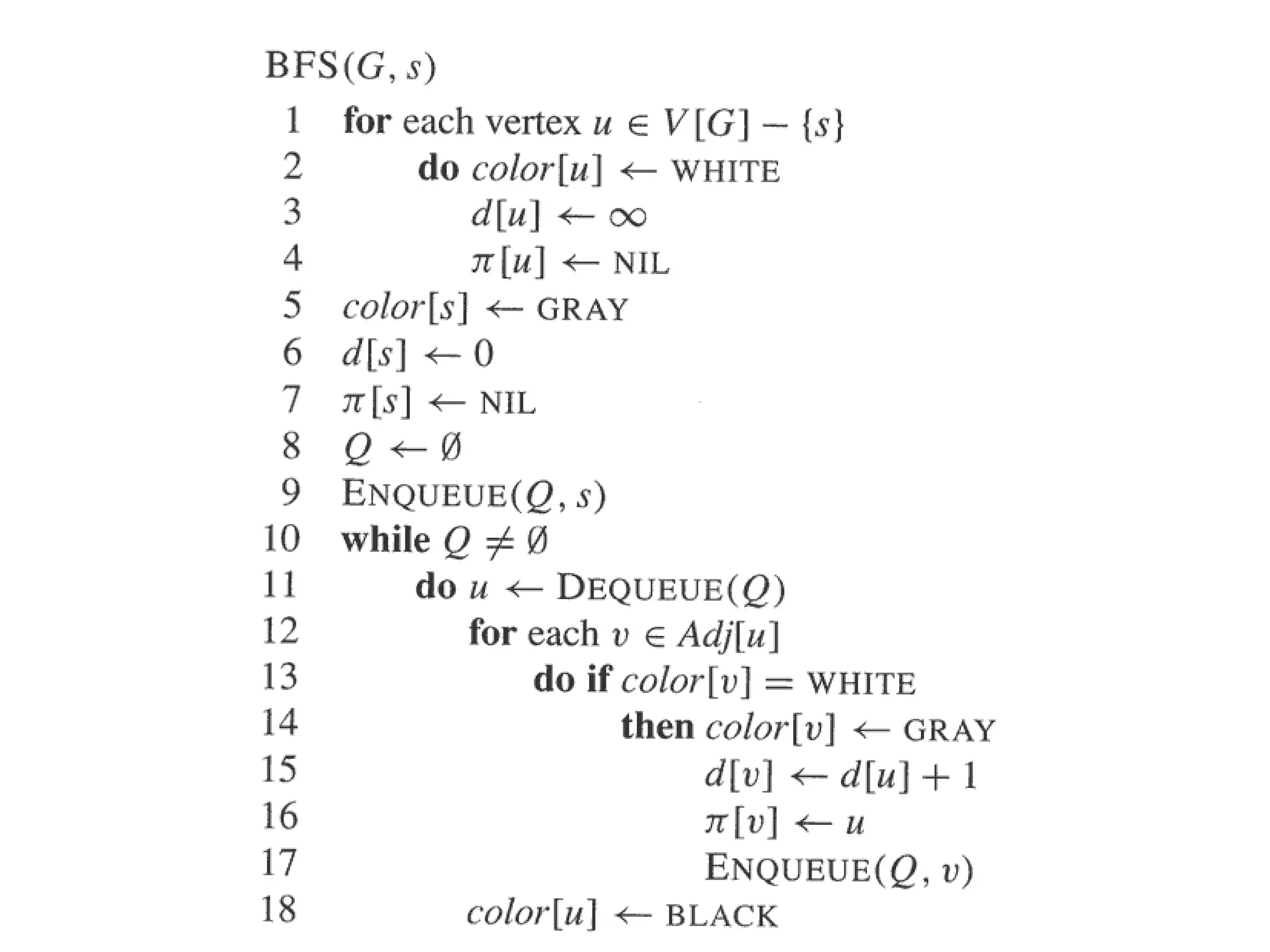
• The breadth-first-searchprocedure BFS assumes that
the input graph G = (V,E) is represented using adjacency
lists.
• It maintains several additional data structures with each
vertex in the graph.
• The color of each vertex u ϵ V is stored in the variable
color[u], and the predecessor of u is stored in the
variable pi[u].
• If u has no predecessor (e.g. u is s or u has not been
discovered), then pi[u] = NIL.
• The distance from the source s to vertex u computed by
the algorithm is stored in d[u].
BFS(Breadth first search)
BFS(Breadth first search)
20.
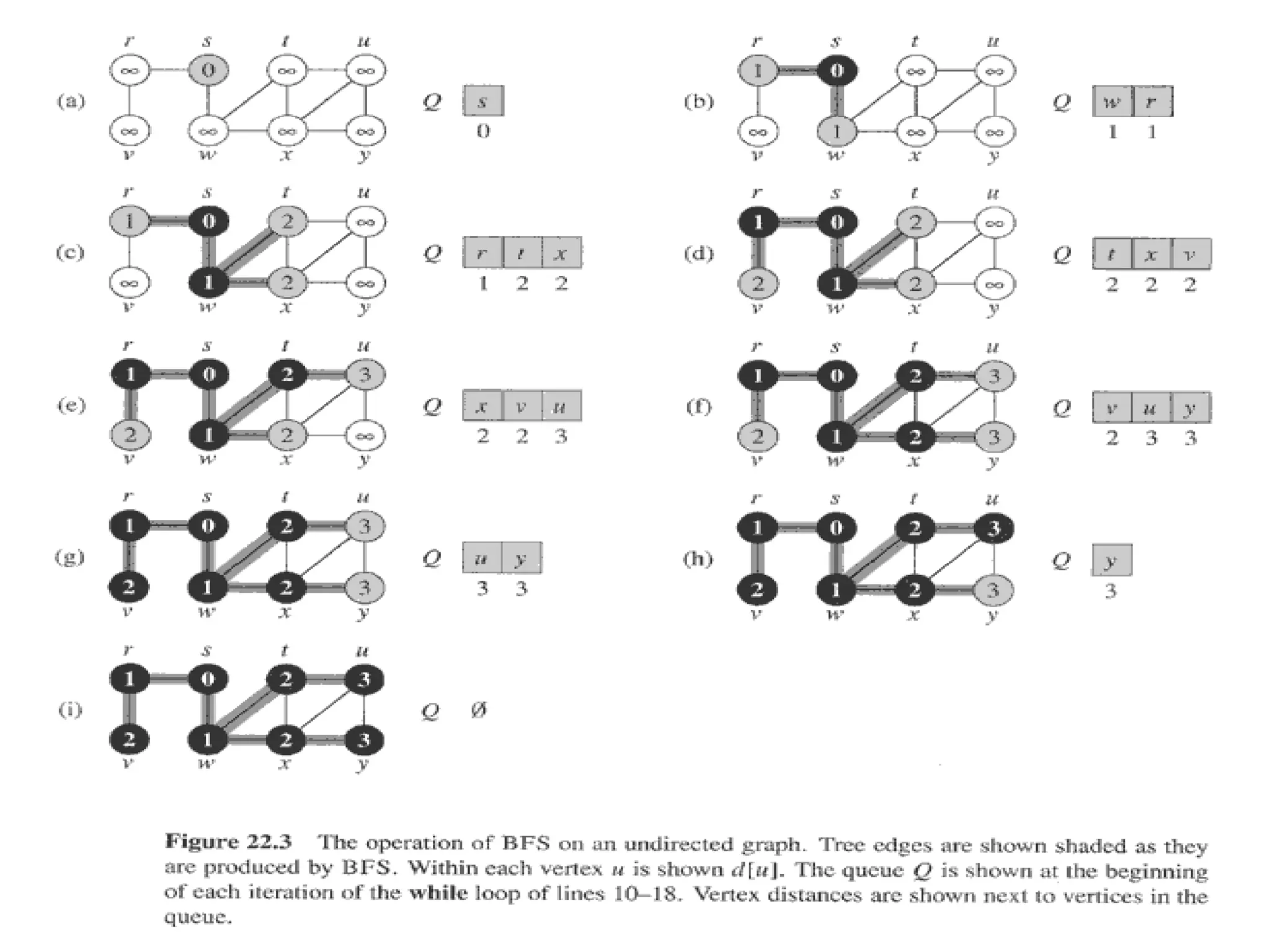
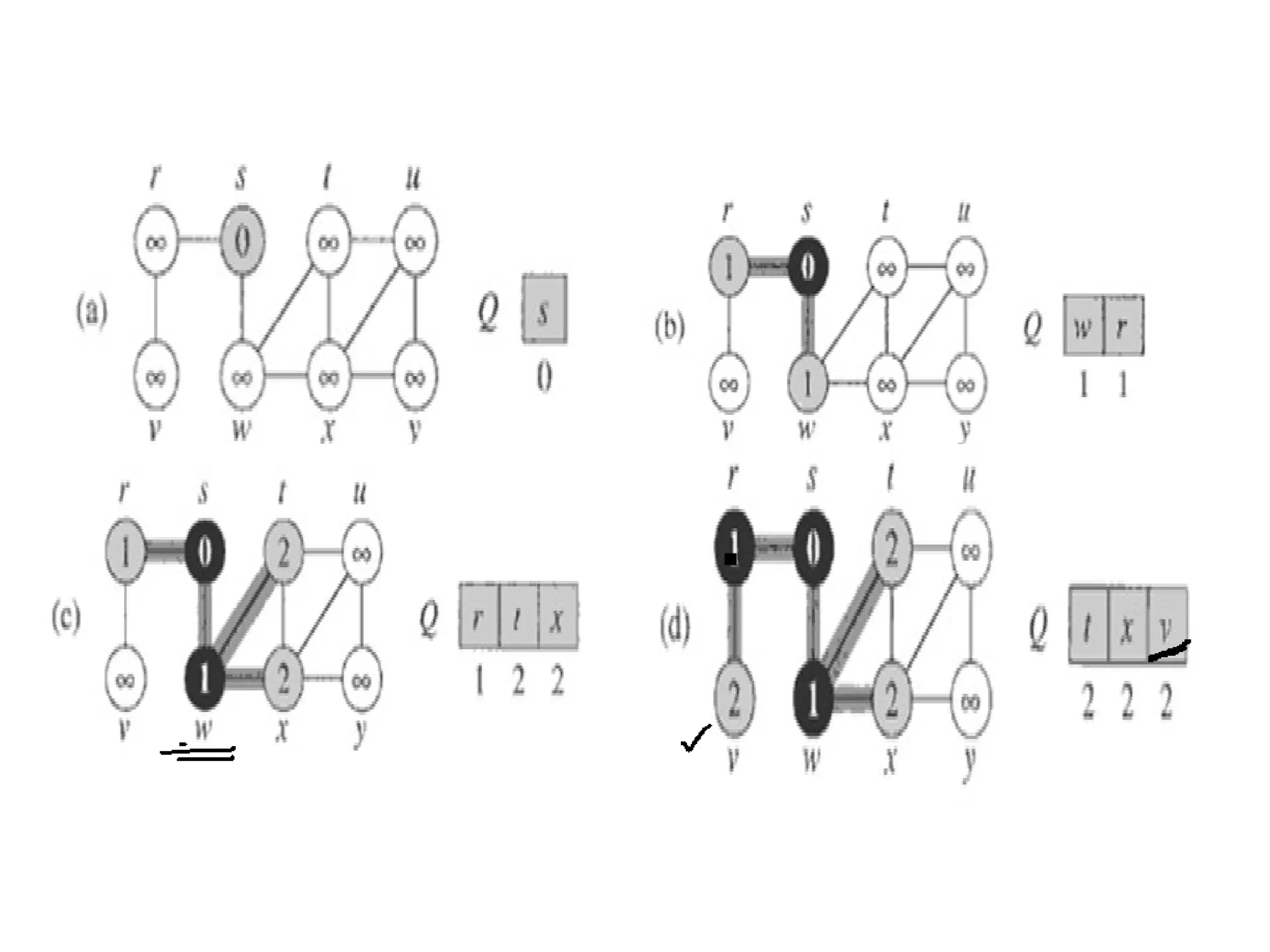
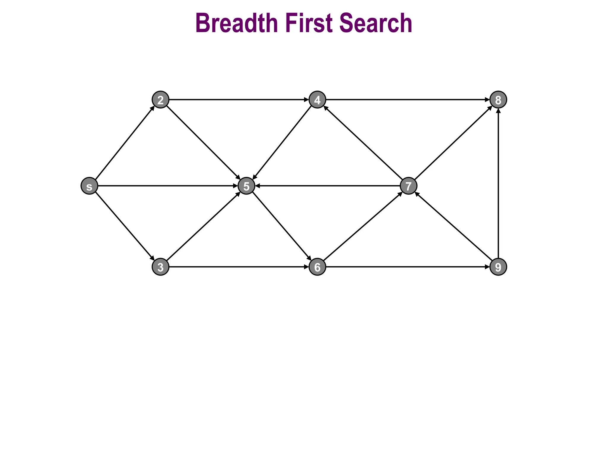
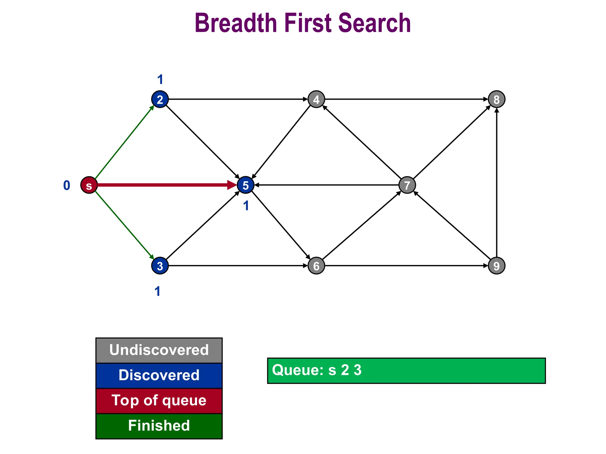
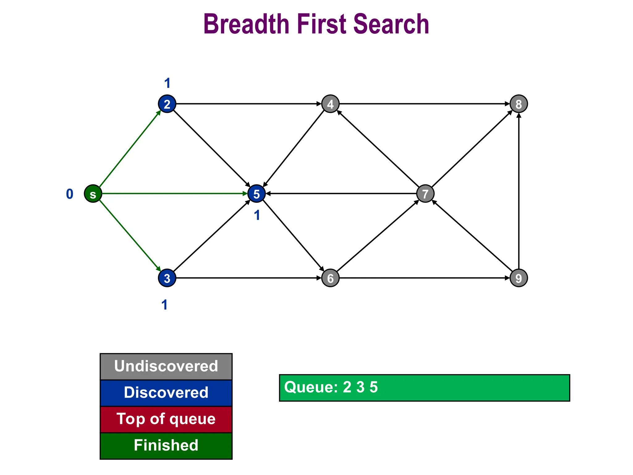
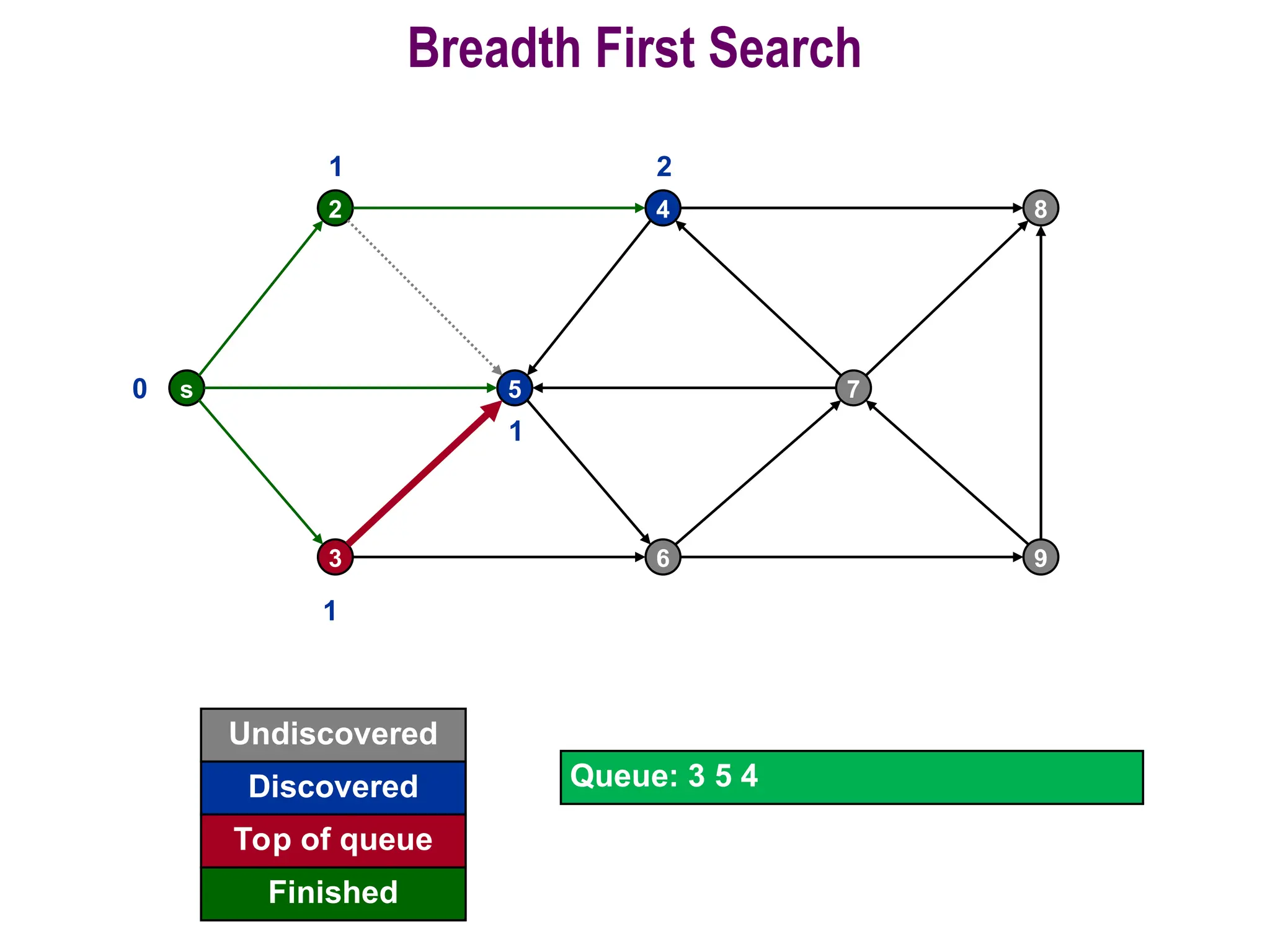
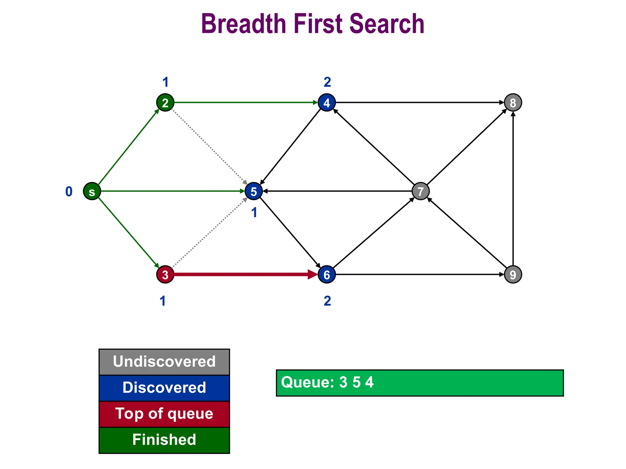
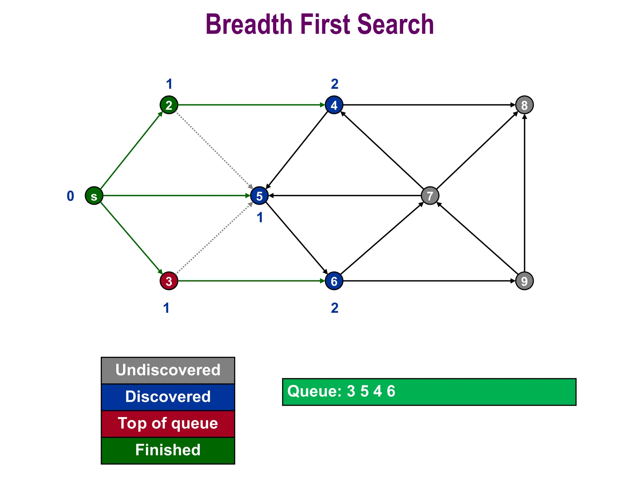
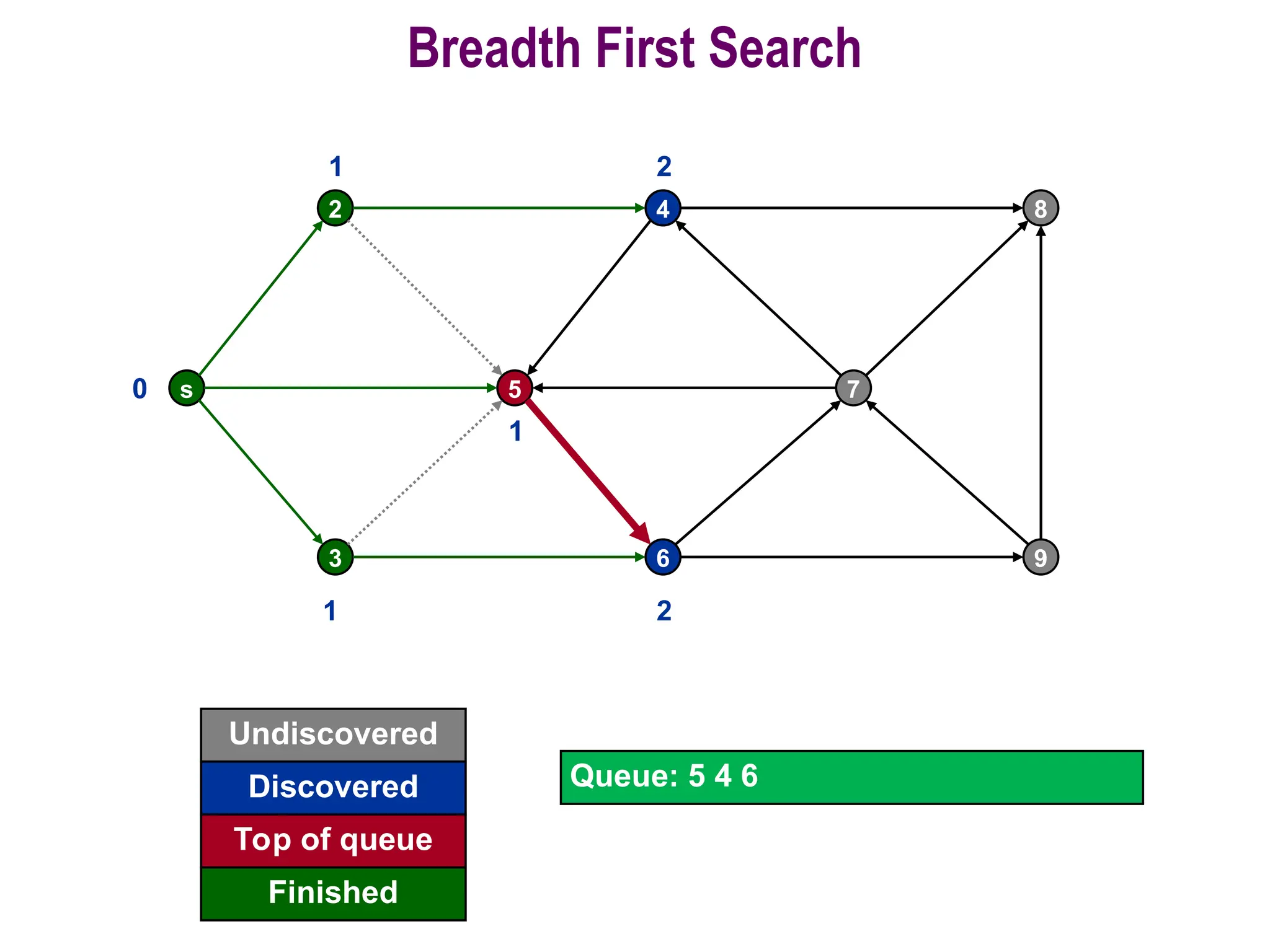
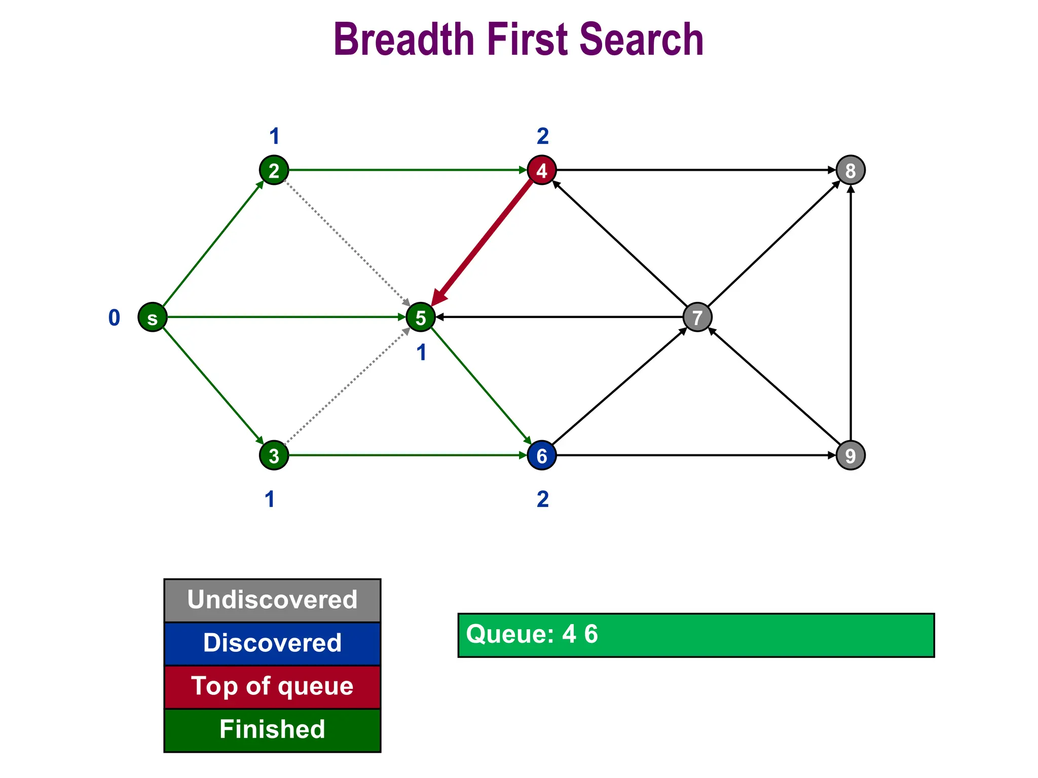
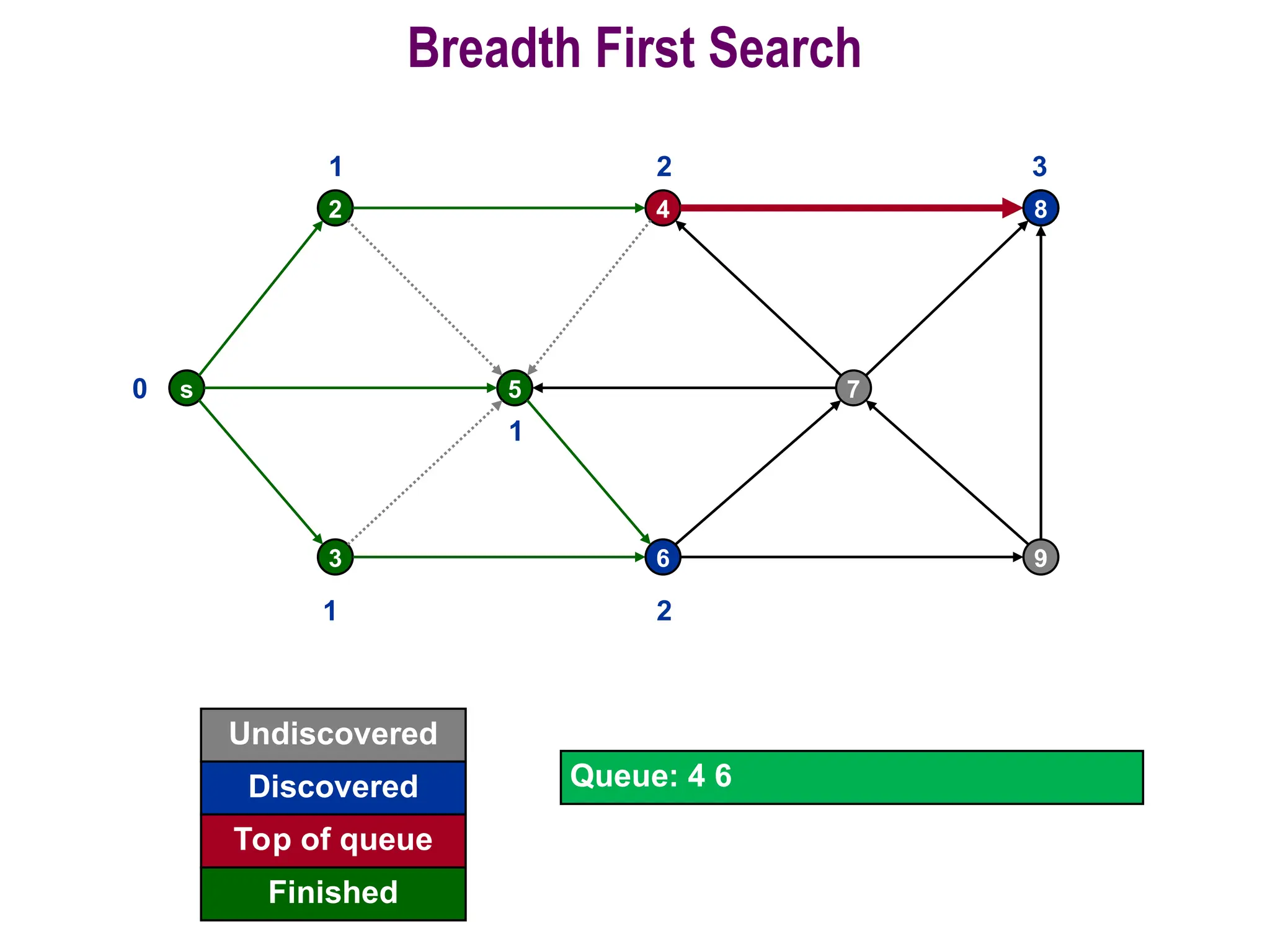
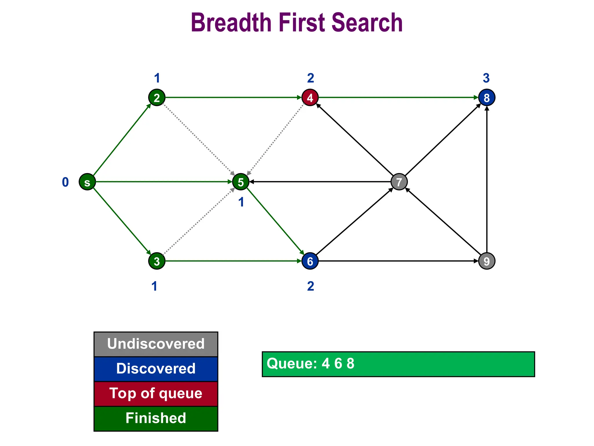
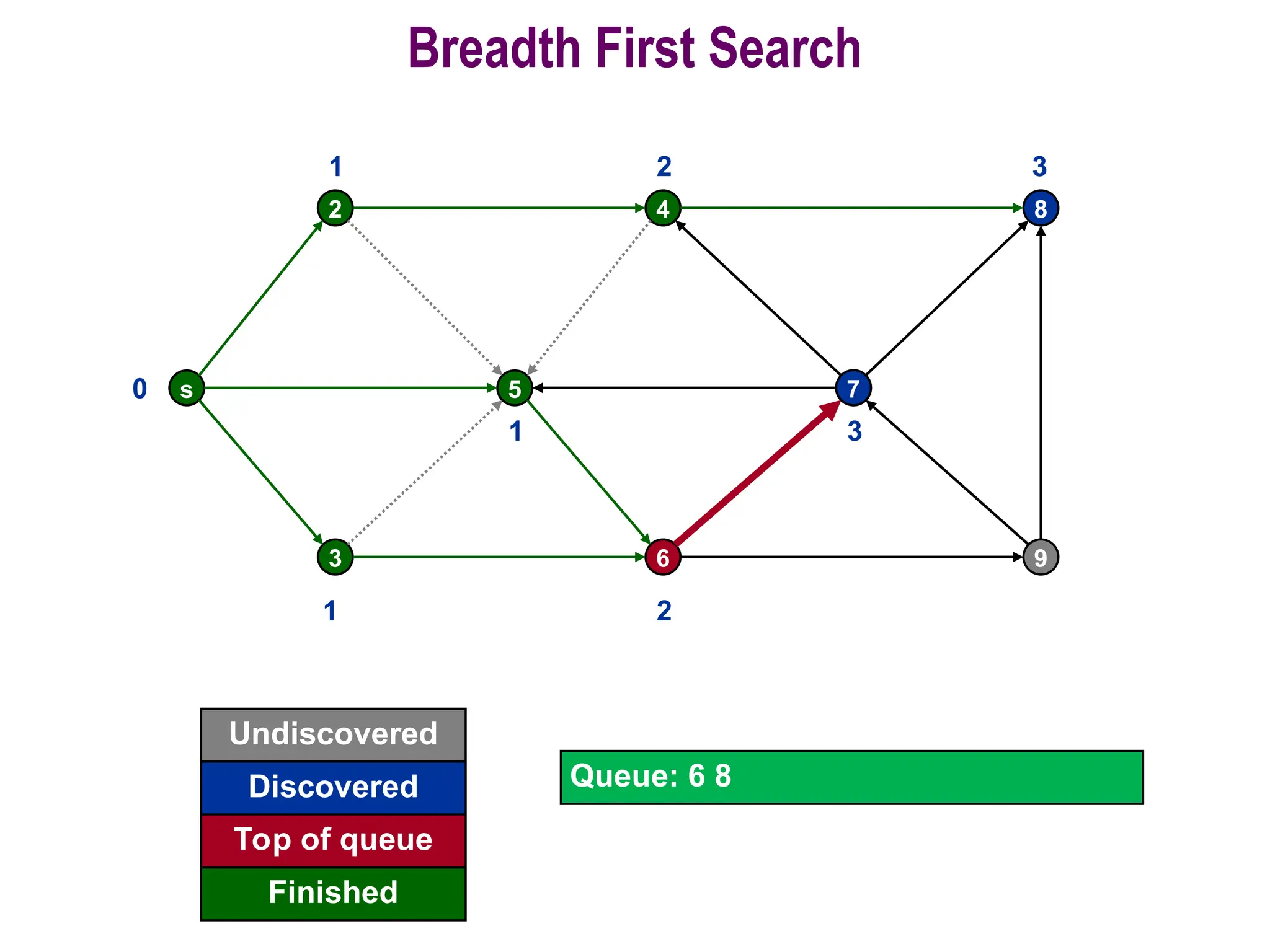
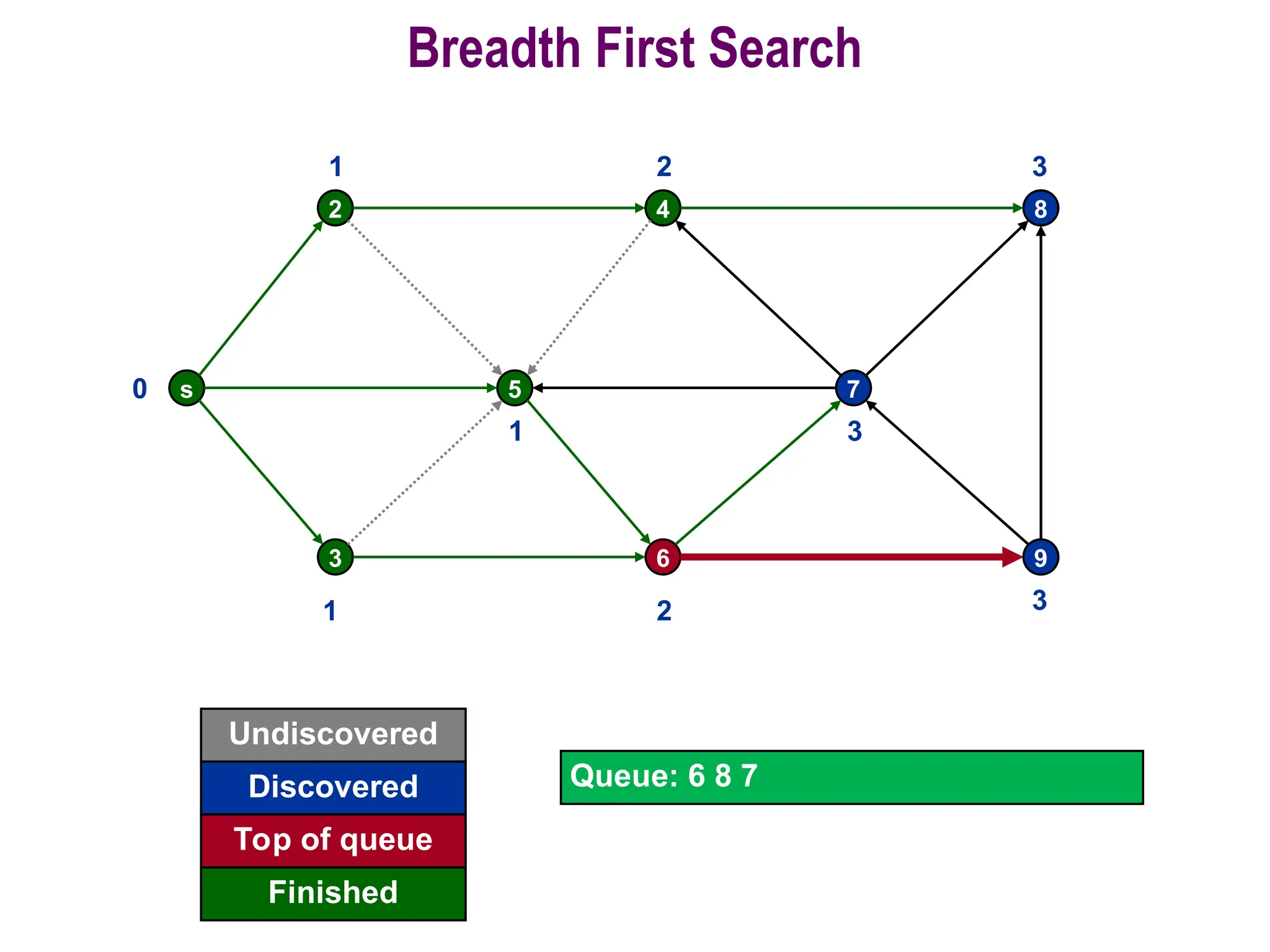
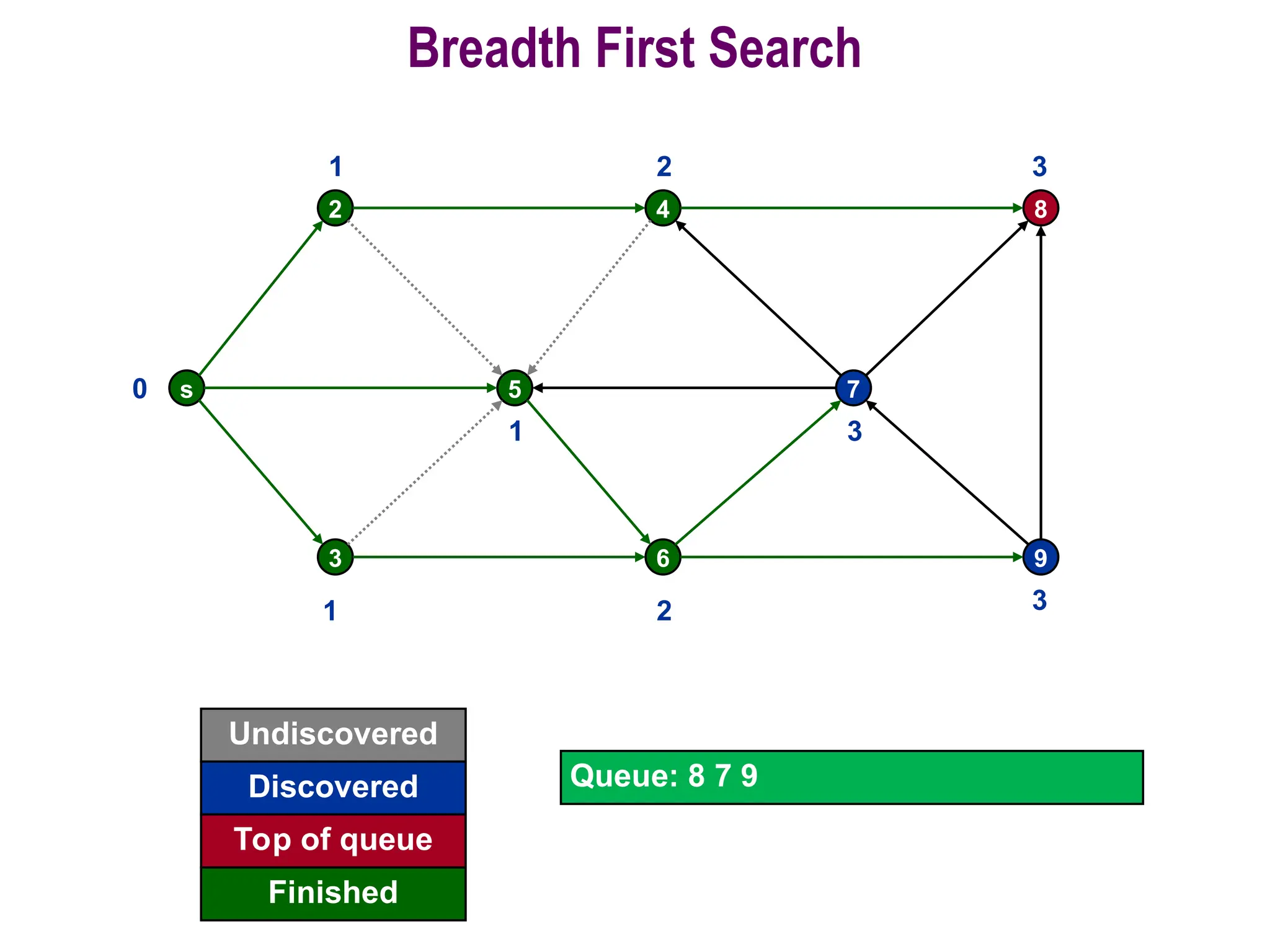
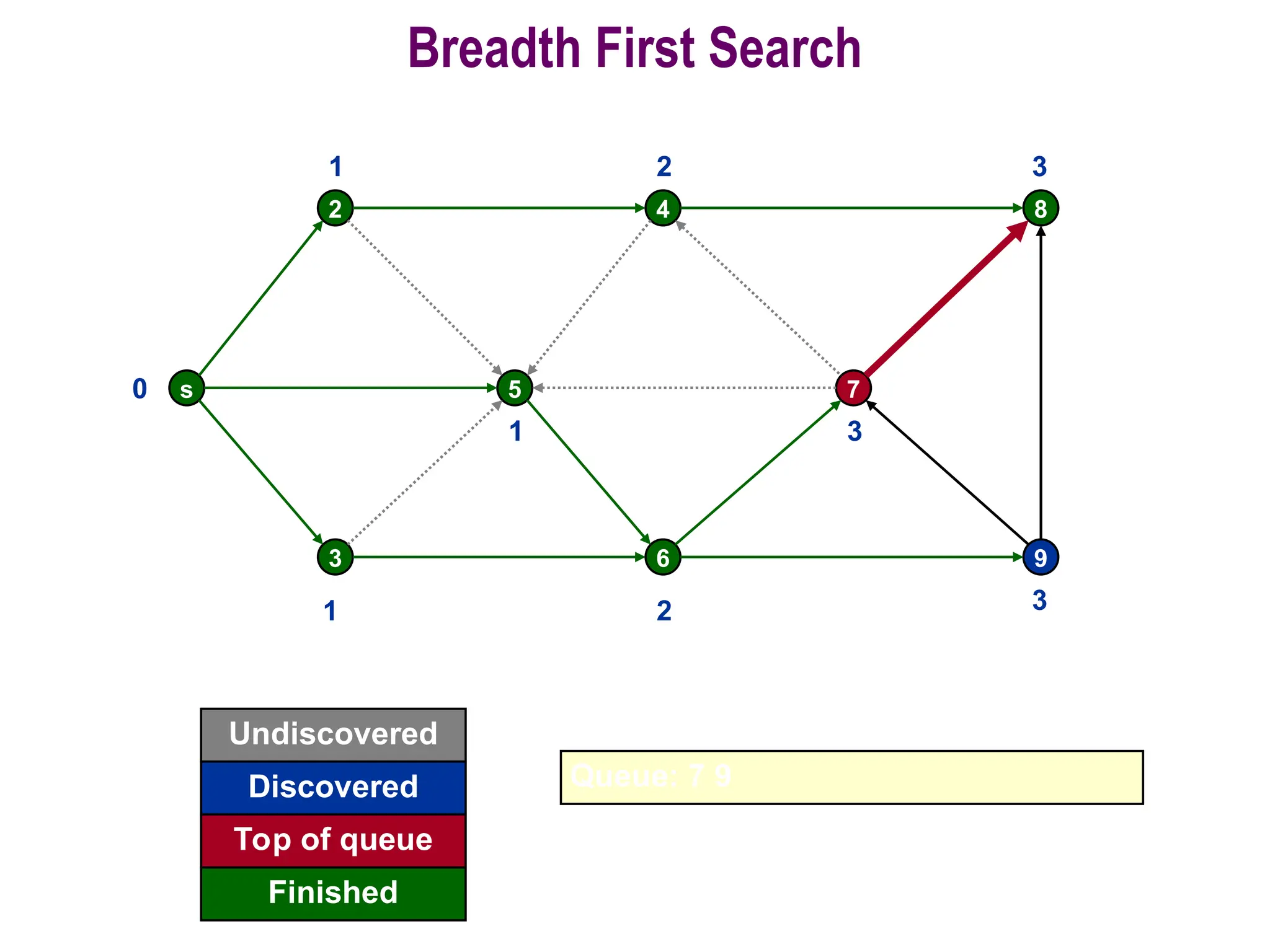
• The algorithmalso uses a FIFO queue Q to
manage the set of gray vertices.
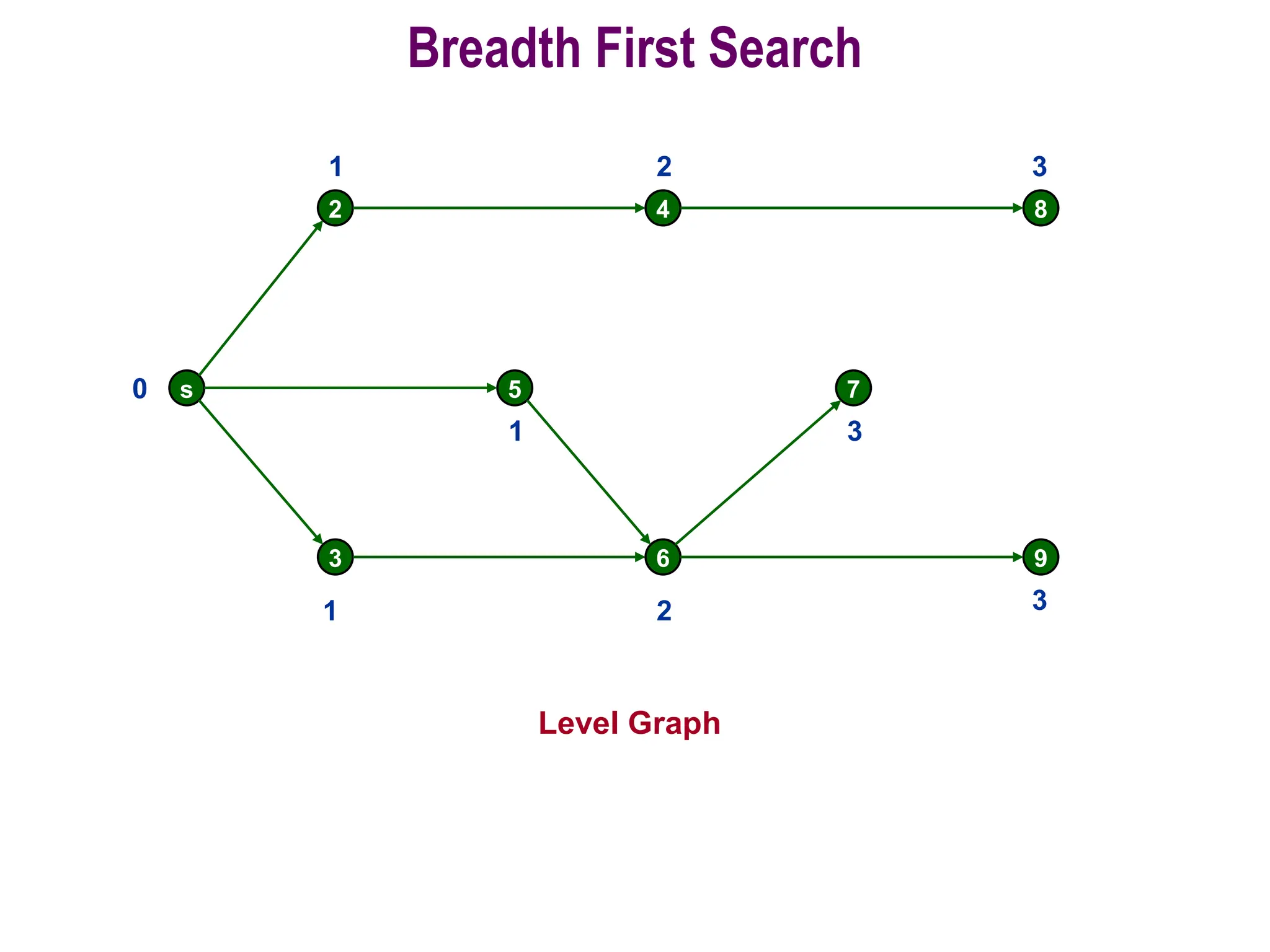
• BFS starts at a given vertex (Source), which is at
level 0.
• In first stage we will visit all vertices at level 1,all
white vertices which are adjacent to source.
• These are colored as grey and added to the
queue. Source is colored black.
• D[v] value of all these vertices is increased by 1.
(D[v] is distance of v from source.)
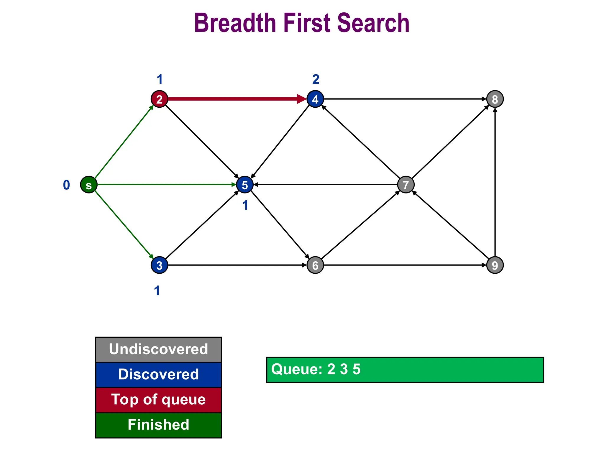
• Now visit all vertices at second level.
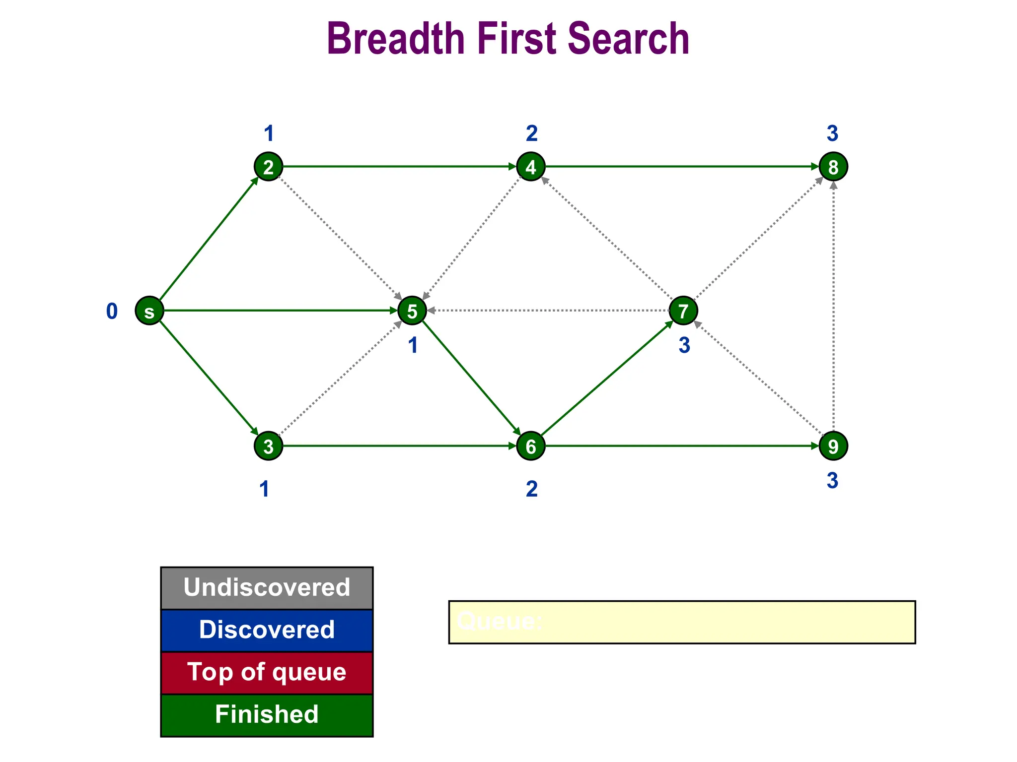
• Once vertex is explored it is colored black and is
deleted from queue.
• The process stops when queue is empty.
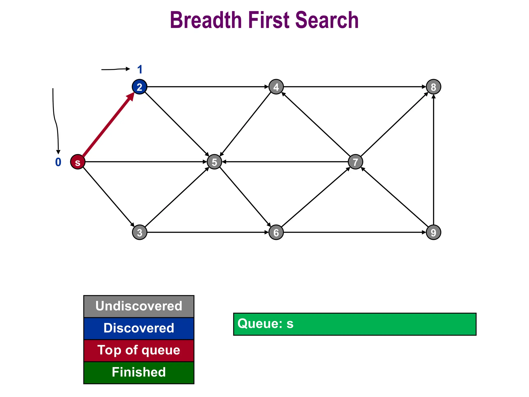
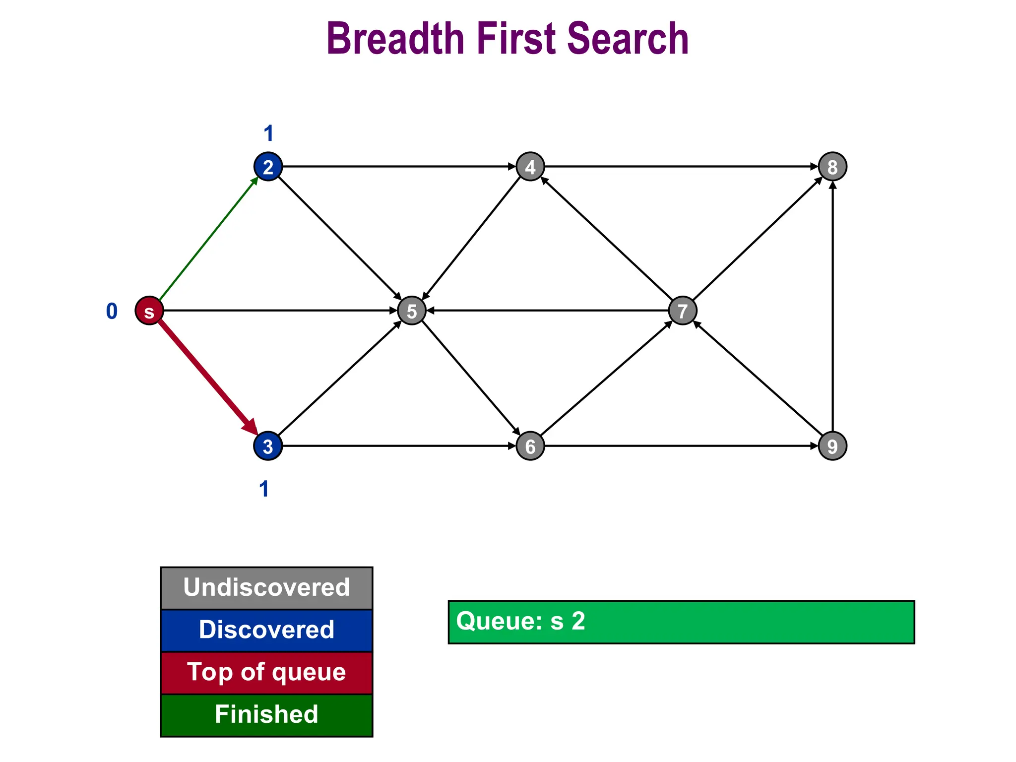
• Lines 1-4paint every vertex white, set d[u] to be
infinity for each vertex u, and set the parent of
every vertex to be NIL.
• Line 5 paints the source vertex s gray, since it is
considered to be discovered when the procedure
begins.
• Line 6 initializes d[s] to be 0, and line 7 sets the
predecessor of the source to be NIL.
• Lines 8-9 initialize Q to the queue containing just
the vertex s.
Working of BFS
Working of BFS
23.
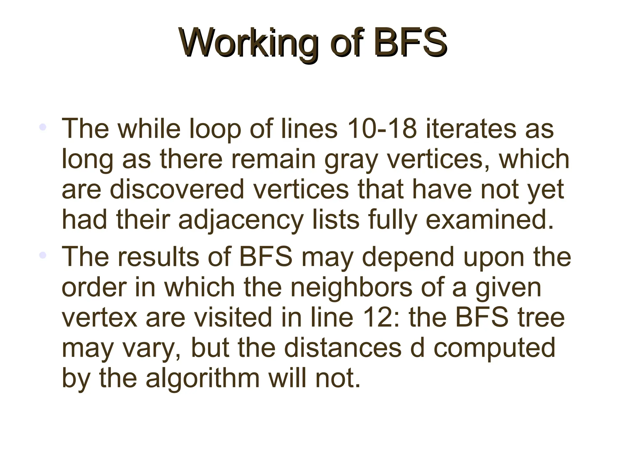
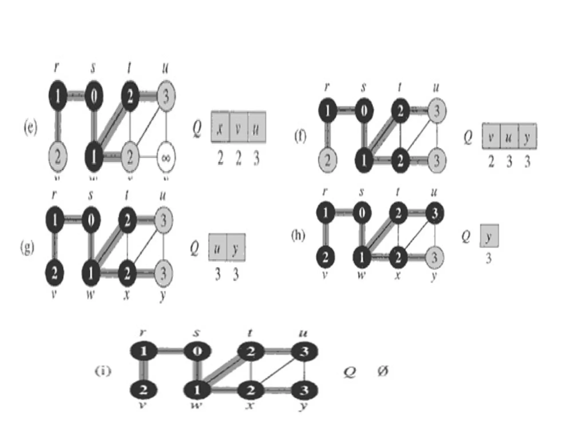
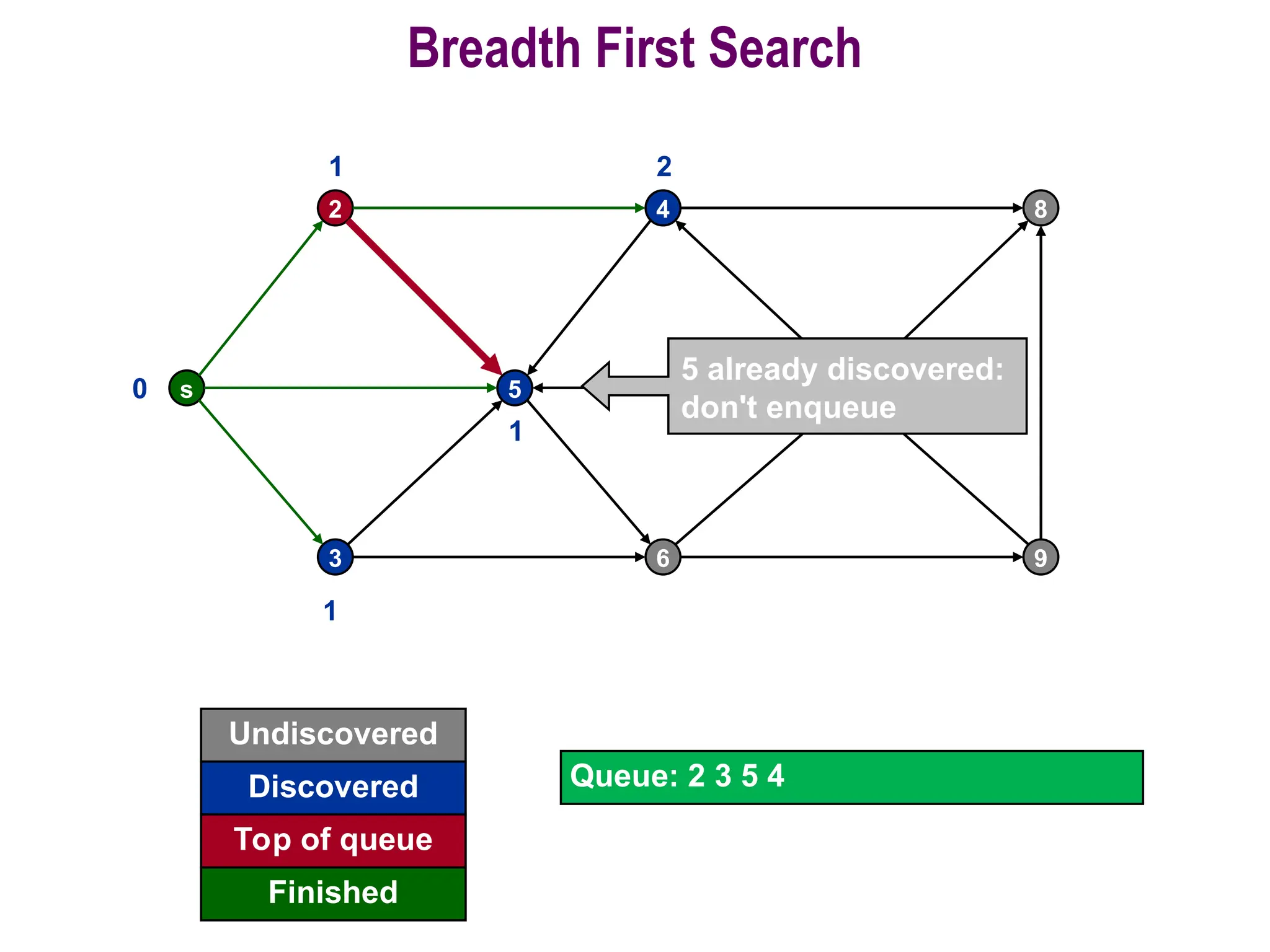
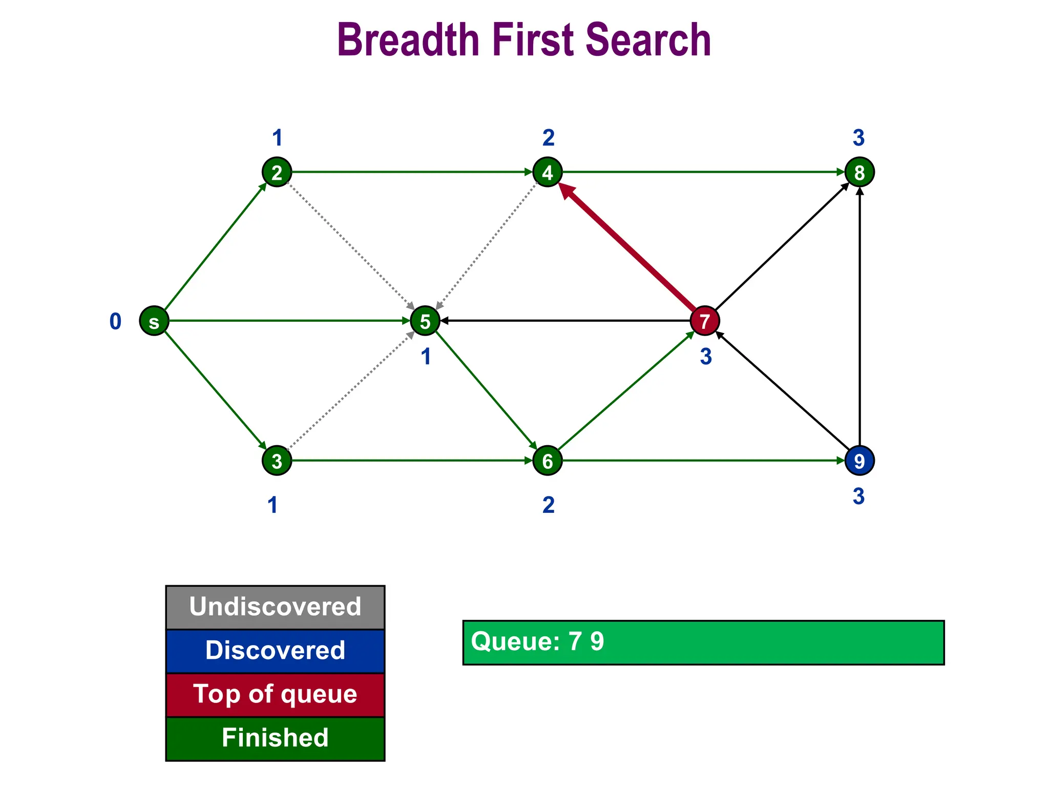
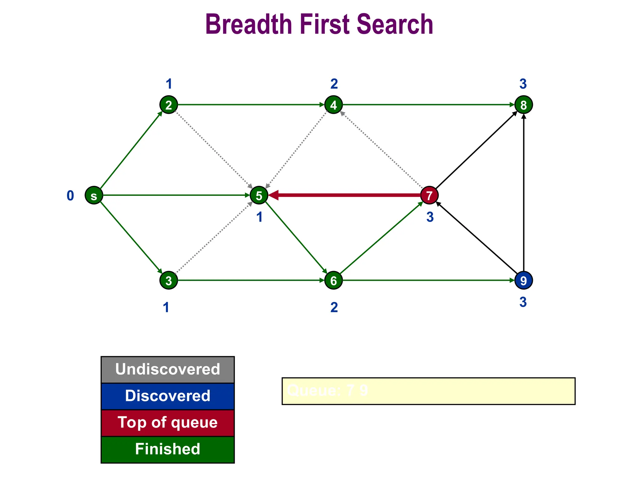
• The whileloop of lines 10-18 iterates as
long as there remain gray vertices, which
are discovered vertices that have not yet
had their adjacency lists fully examined.
• The results of BFS may depend upon the
order in which the neighbors of a given
vertex are visited in line 12: the BFS tree
may vary, but the distances d computed
by the algorithm will not.
Working of BFS
Working of BFS
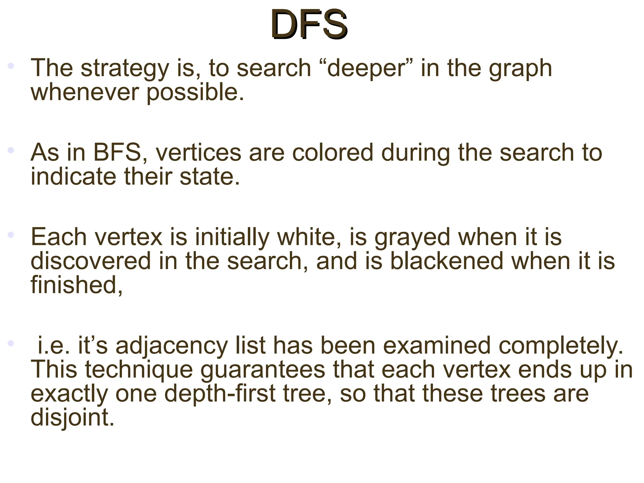
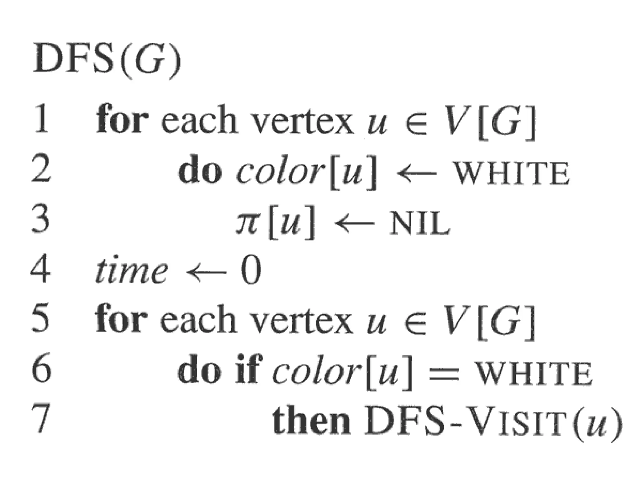
• The strategyis, to search “deeper” in the graph
whenever possible.
• As in BFS, vertices are colored during the search to
indicate their state.
• Each vertex is initially white, is grayed when it is
discovered in the search, and is blackened when it is
finished,
• i.e. it’s adjacency list has been examined completely.
This technique guarantees that each vertex ends up in
exactly one depth-first tree, so that these trees are
disjoint.
DFS
DFS
59.
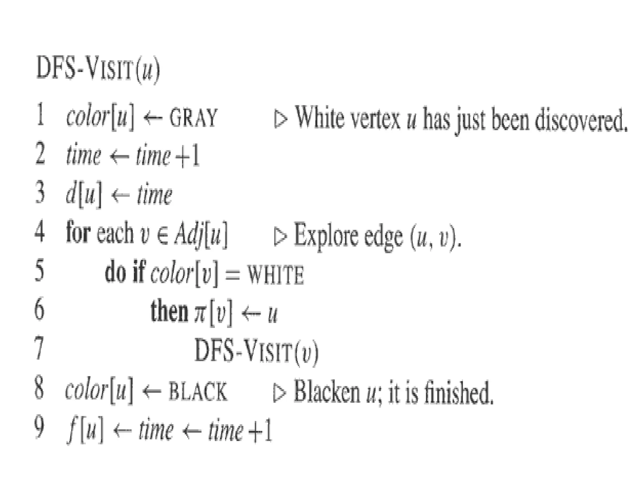
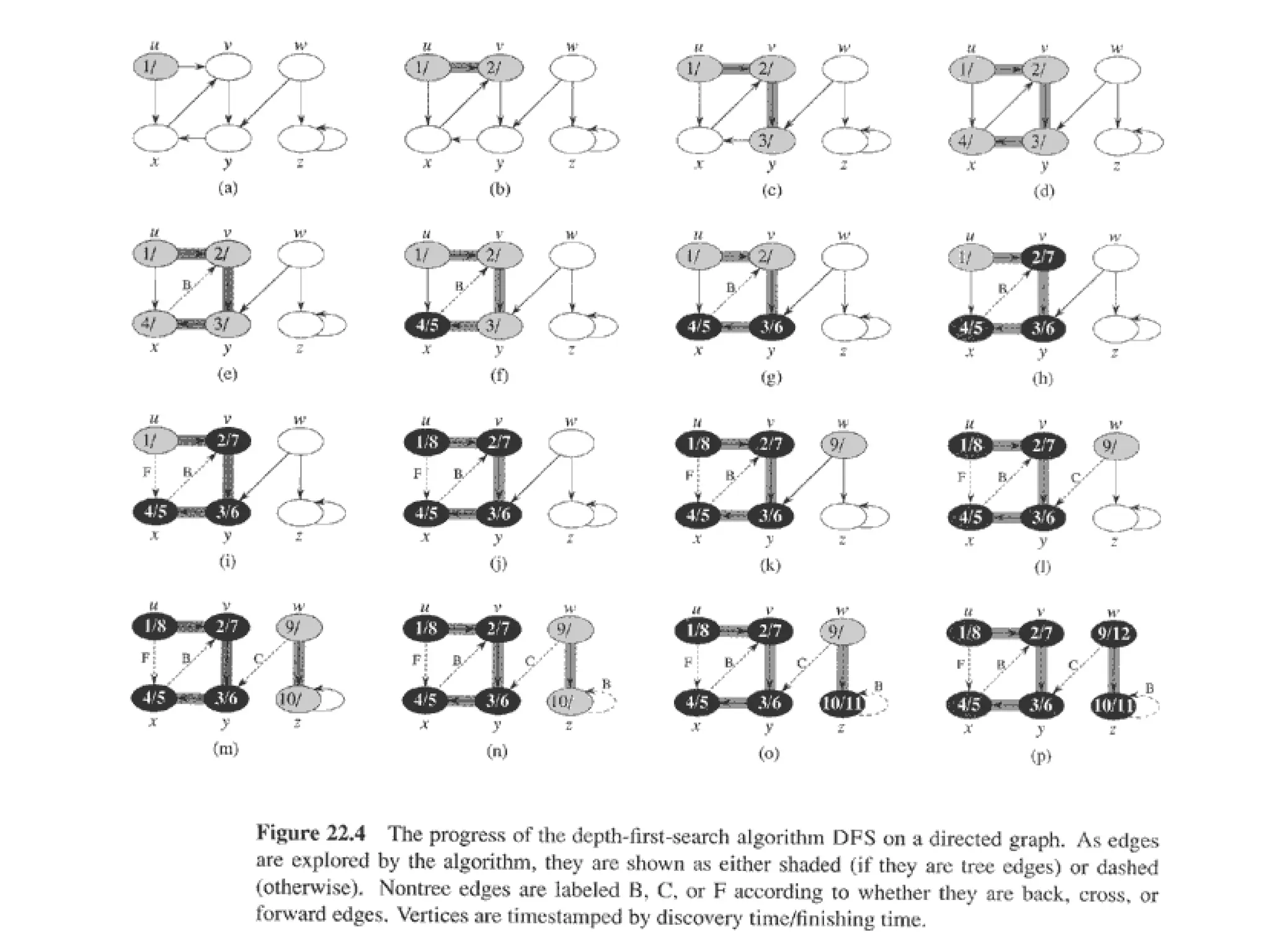
• Besides creatinga depth-first forest, DFS
also timestamps each vertex.
• Each vertex u has 2 timestamps: the first
timestamp d[u] records when u is first
discovered (and grayed), and the second
timestamp f[u] records when the search
finishes examining u’s adjacency list (and
blackens u).
• These timestamps are used in many graph
algorithms and are generally helpful in
reasoning about the behavior of DFS.
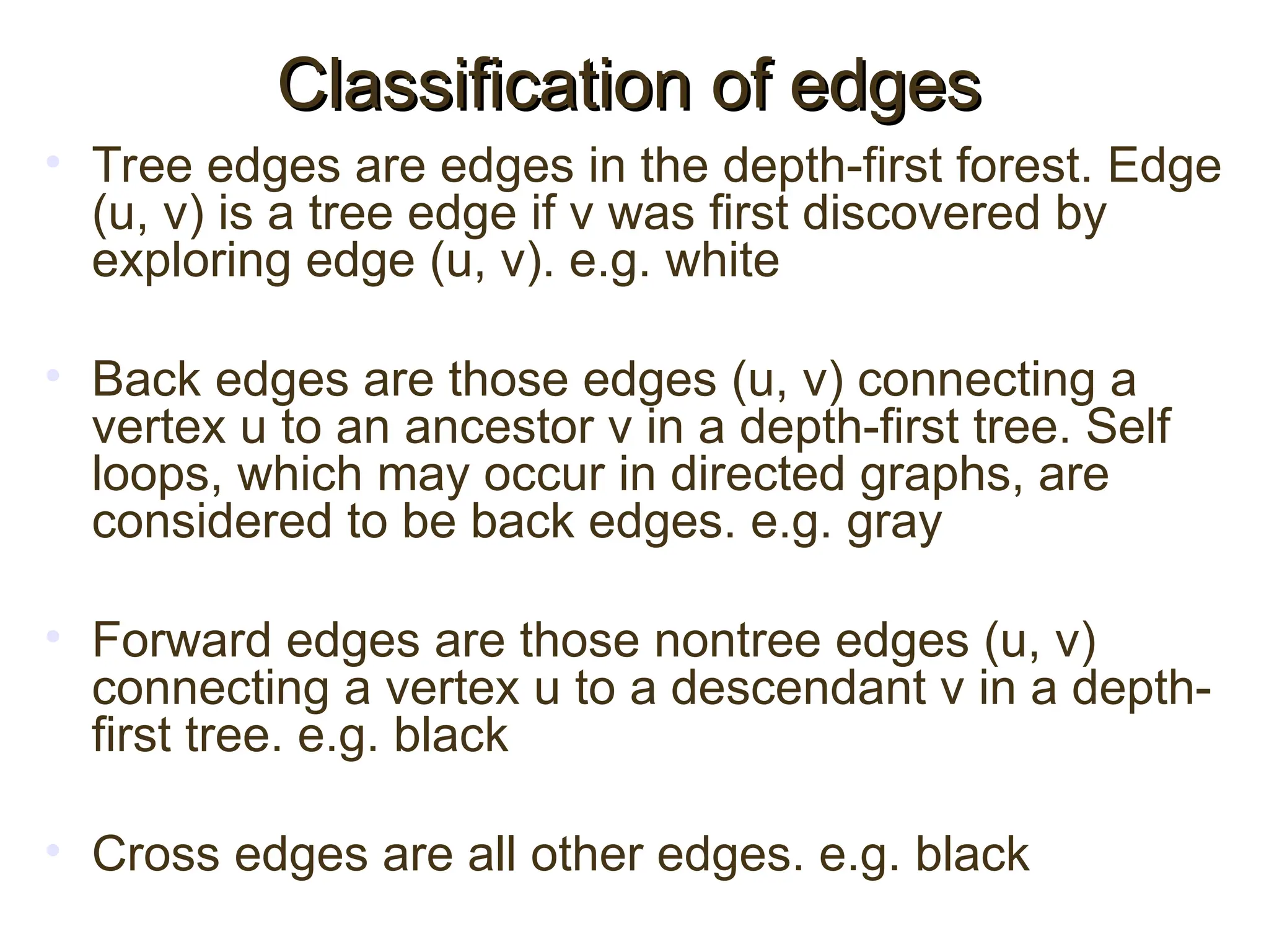
• Tree edgesare edges in the depth-first forest. Edge
(u, v) is a tree edge if v was first discovered by
exploring edge (u, v). e.g. white
• Back edges are those edges (u, v) connecting a
vertex u to an ancestor v in a depth-first tree. Self
loops, which may occur in directed graphs, are
considered to be back edges. e.g. gray
• Forward edges are those nontree edges (u, v)
connecting a vertex u to a descendant v in a depth-
first tree. e.g. black
• Cross edges are all other edges. e.g. black
Classification of edges
Classification of edges
64.
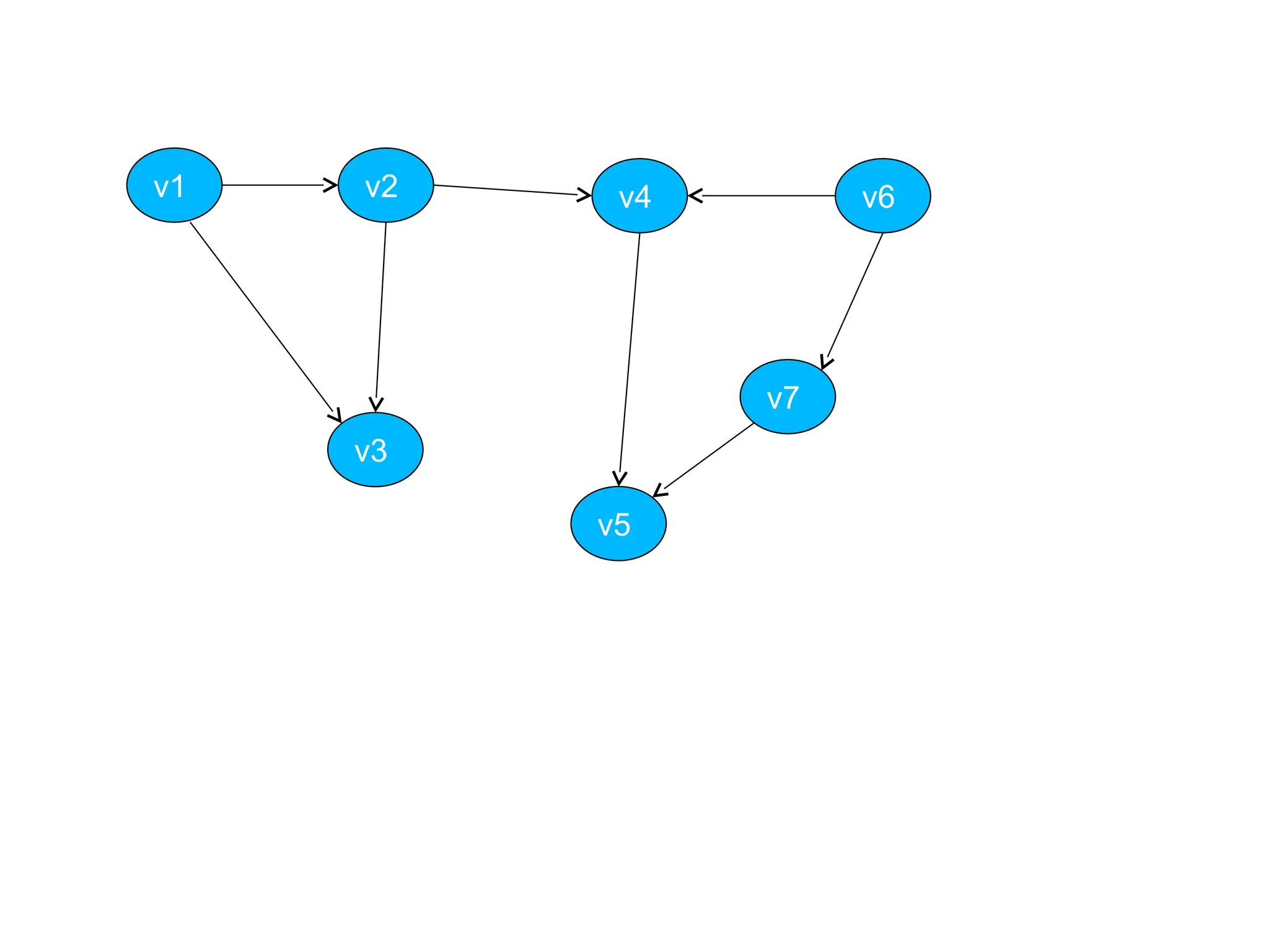
• A topologicalsort of a directed acyclic
graph (dag) G = (V, E) is a linear ordering
of all its vertices such that if G contains an
edge (u, v), then u appears before v in the
ordering.
Topological sort
Topological sort
65.
Topological Sorting
Topological Sorting
•It is an ordering of vertices of a graph, such that,
if there is a path from u to v in the graph then u
appears before v in the ordering.
• It is clear that a topological ordering is not
possible if the graph has a cycle, since for two
vertices u and v on the cycle, u precedes v and v
precedes u.
• It can also be proved that, for a directed acyclic
graph, there exists a topological ordering of
vertices.
66.
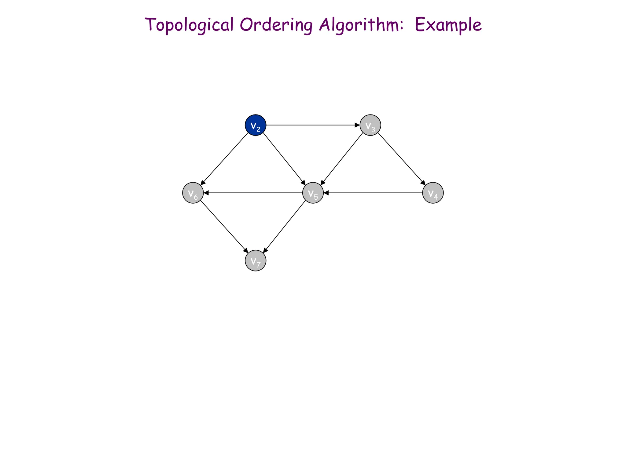
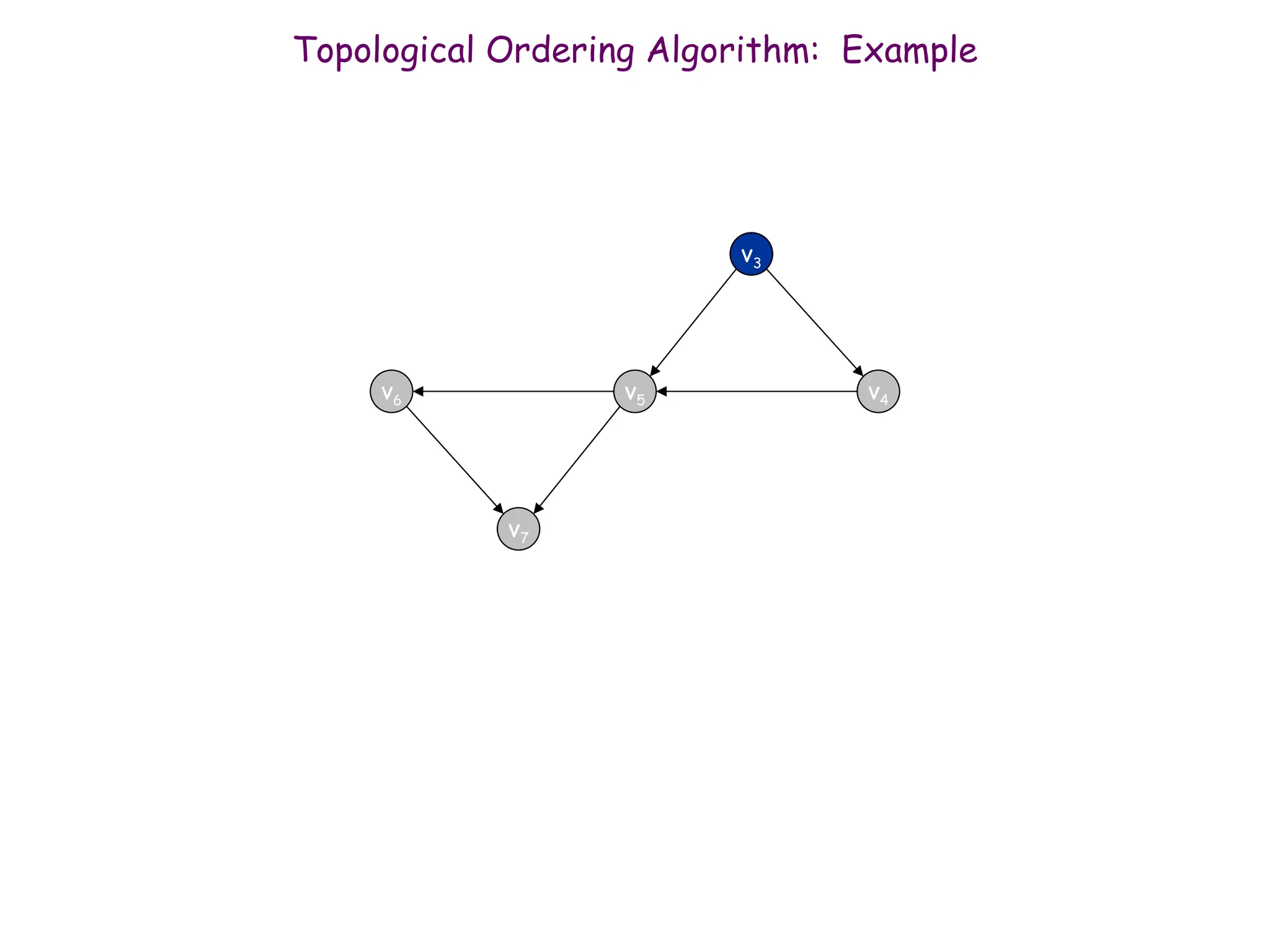
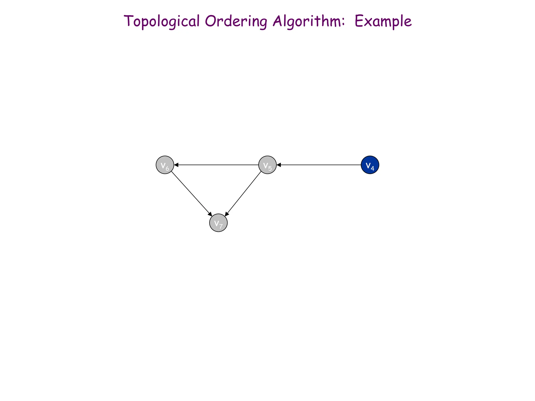
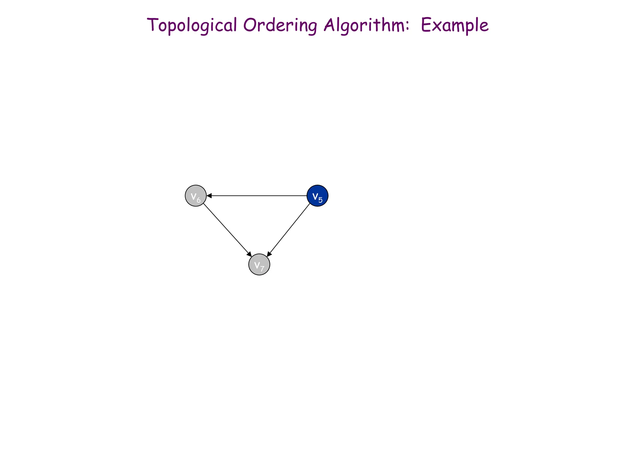
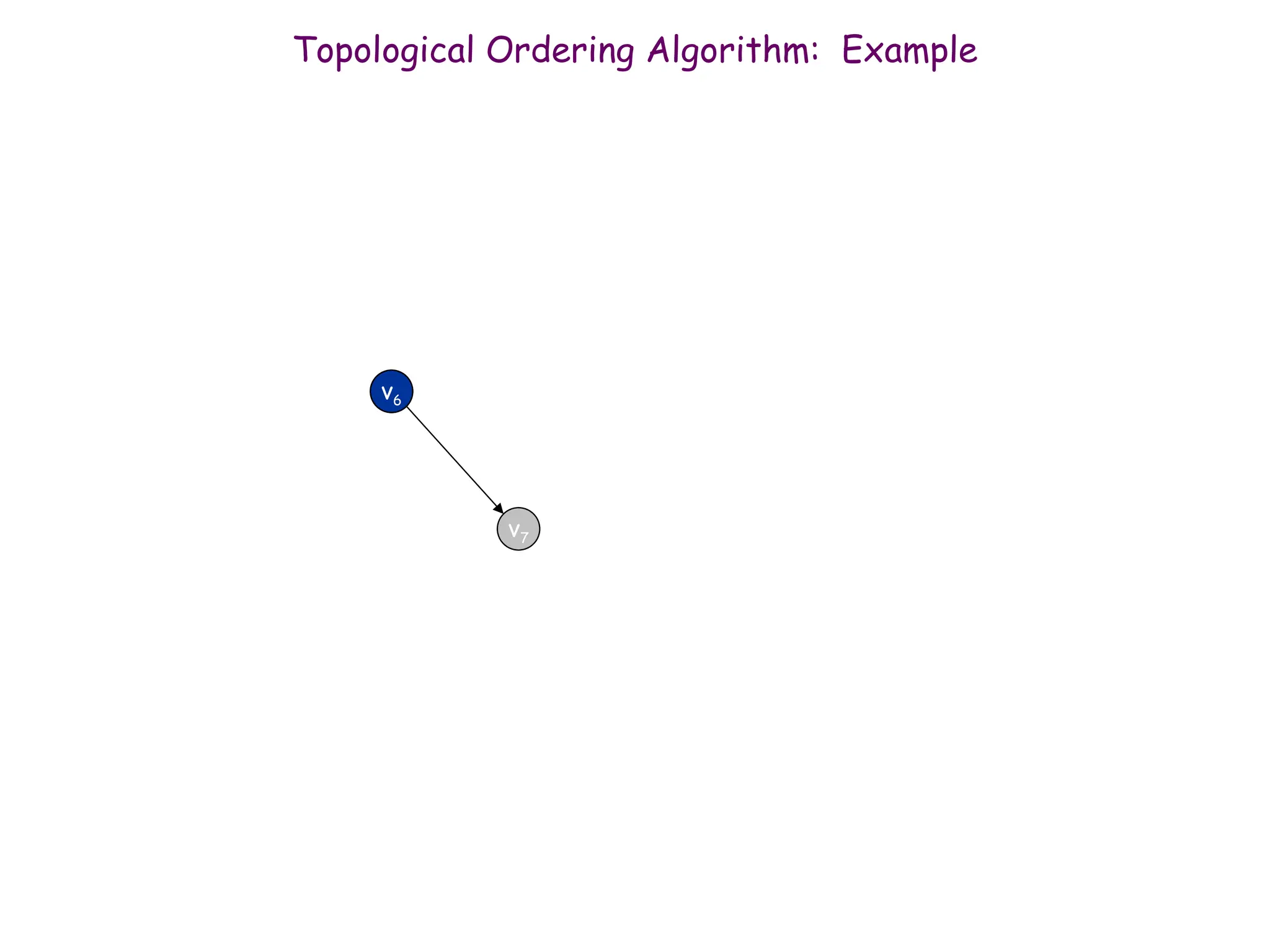
Topological Sorting Algorithm
TopologicalSorting Algorithm
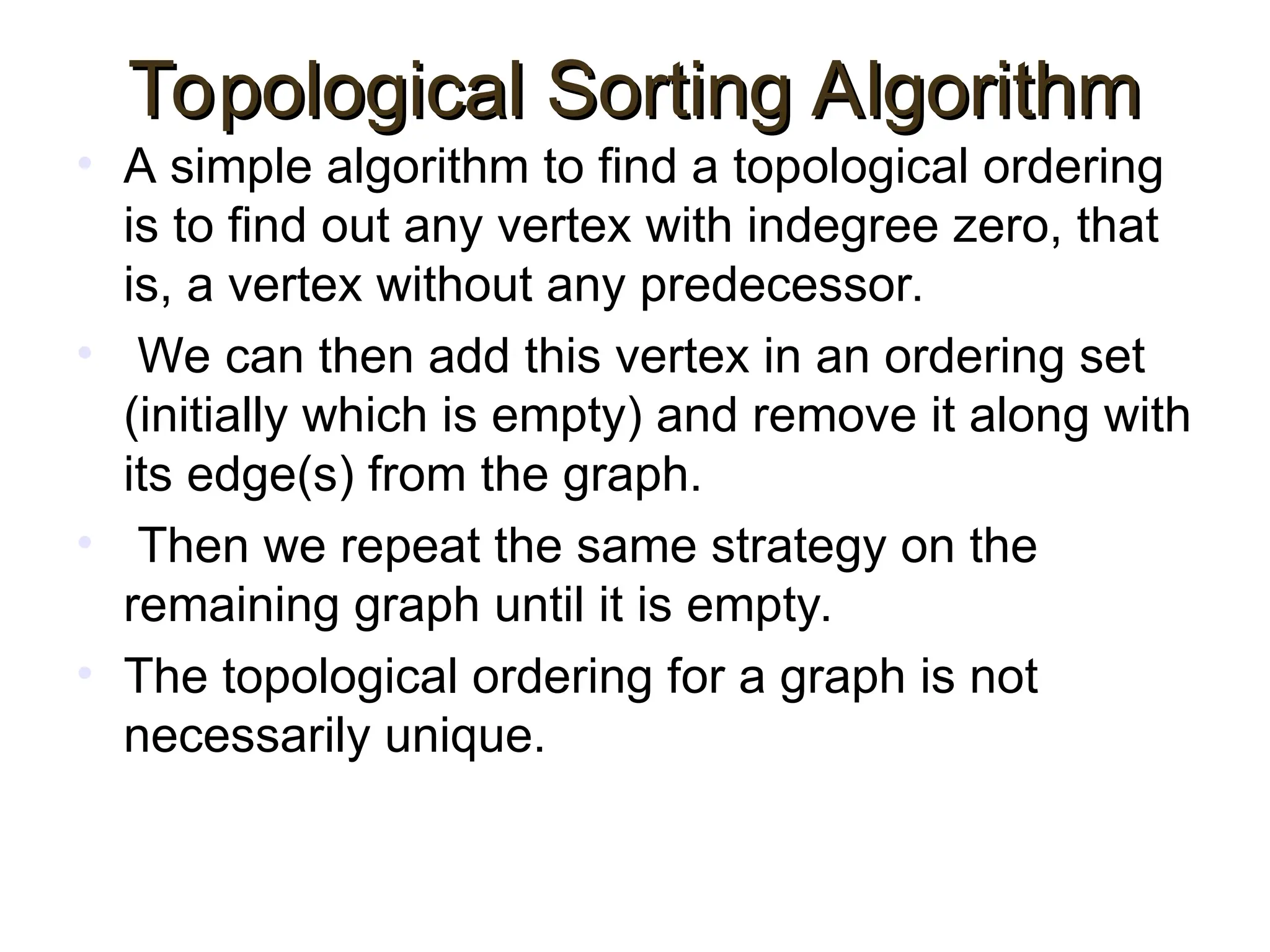
• A simple algorithm to find a topological ordering
is to find out any vertex with indegree zero, that
is, a vertex without any predecessor.
• We can then add this vertex in an ordering set
(initially which is empty) and remove it along with
its edge(s) from the graph.
• Then we repeat the same strategy on the
remaining graph until it is empty.
• The topological ordering for a graph is not
necessarily unique.
68.
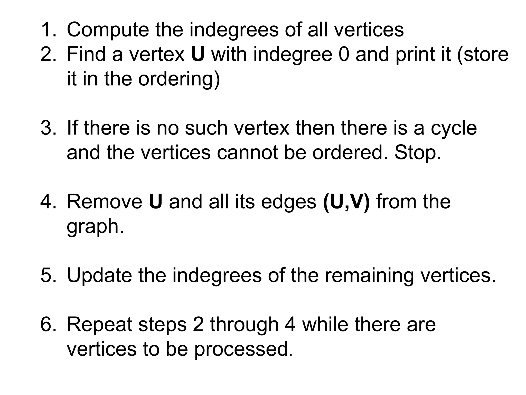
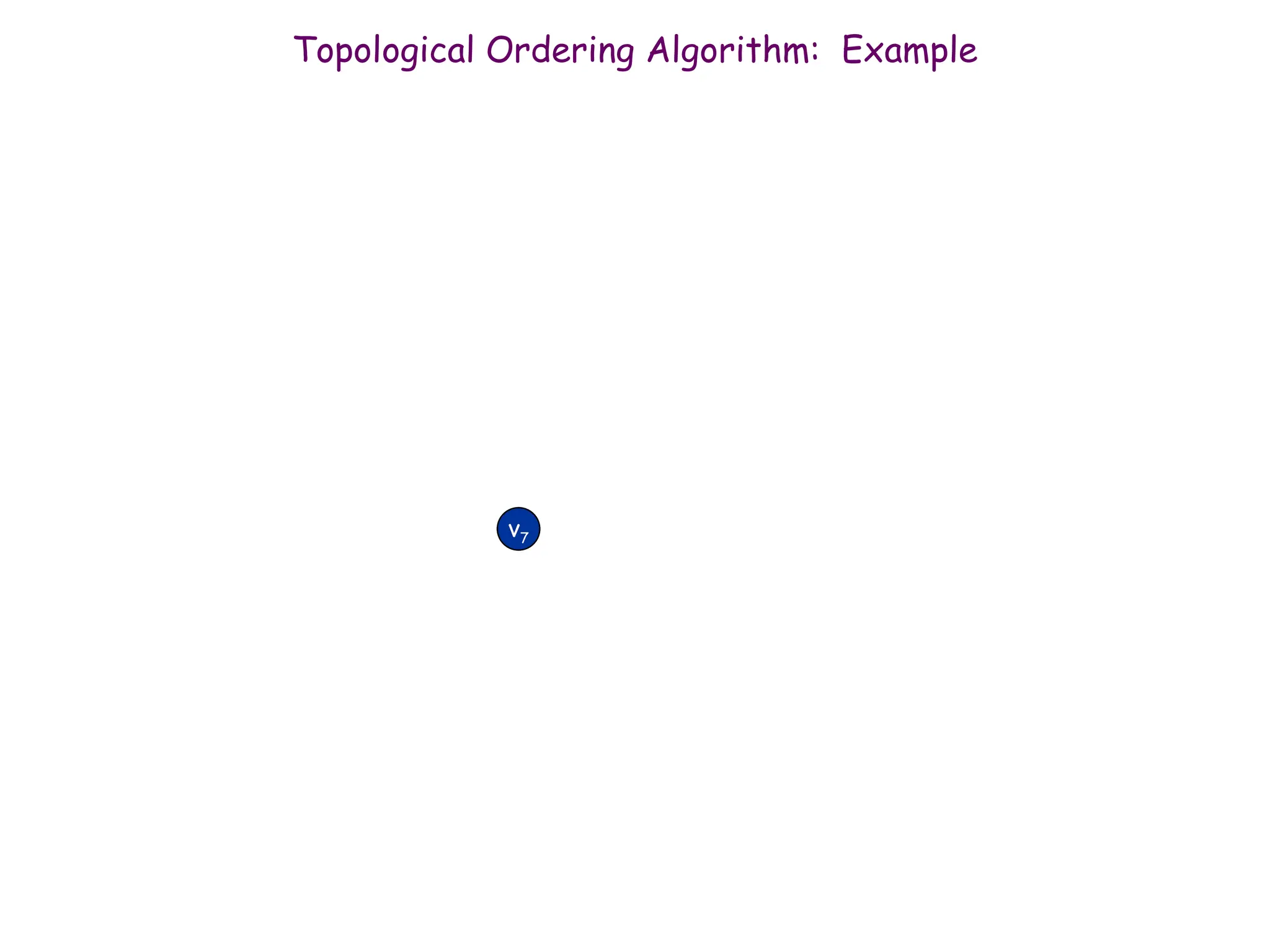
1. Compute theindegrees of all vertices
2. Find a vertex U with indegree 0 and print it (store
it in the ordering)
3. If there is no such vertex then there is a cycle
and the vertices cannot be ordered. Stop.
4. Remove U and all its edges (U,V) from the
graph.
5. Update the indegrees of the remaining vertices.
6. Repeat steps 2 through 4 while there are
vertices to be processed.
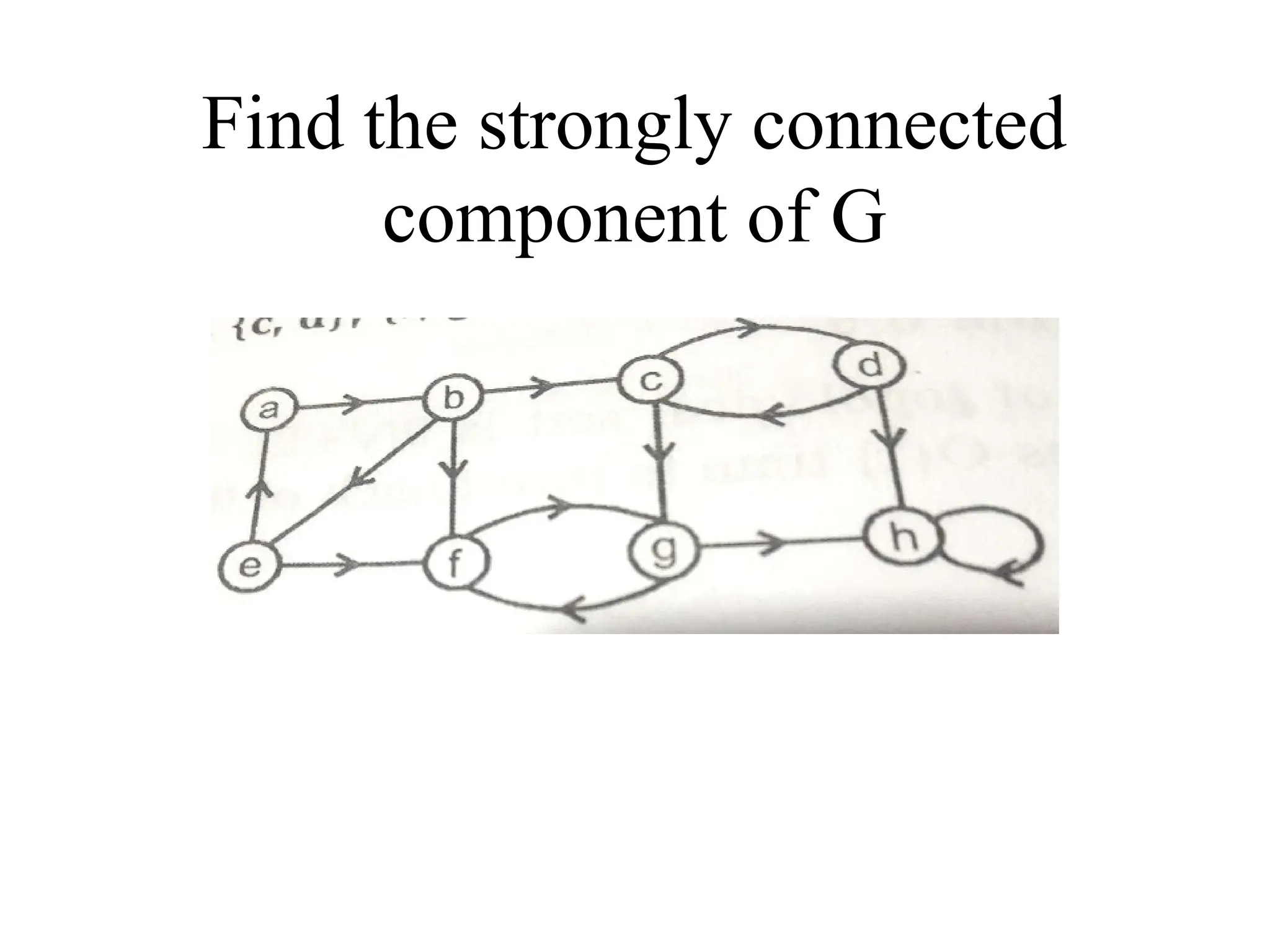
Strongly connected components
•Decomposing a directed graph into its strongly
connected component is application of DFS.
• Two vertices of a directed graph are in the same
component if and only if they are reachable from
each other.
• i.e if u and v are two vertices in the same
component then there is a directed path from u to
v as well as from v to u.
• If u and v are not in same component then, if
there is a directed path from u to v then there is
no directed path from v to u.
78.
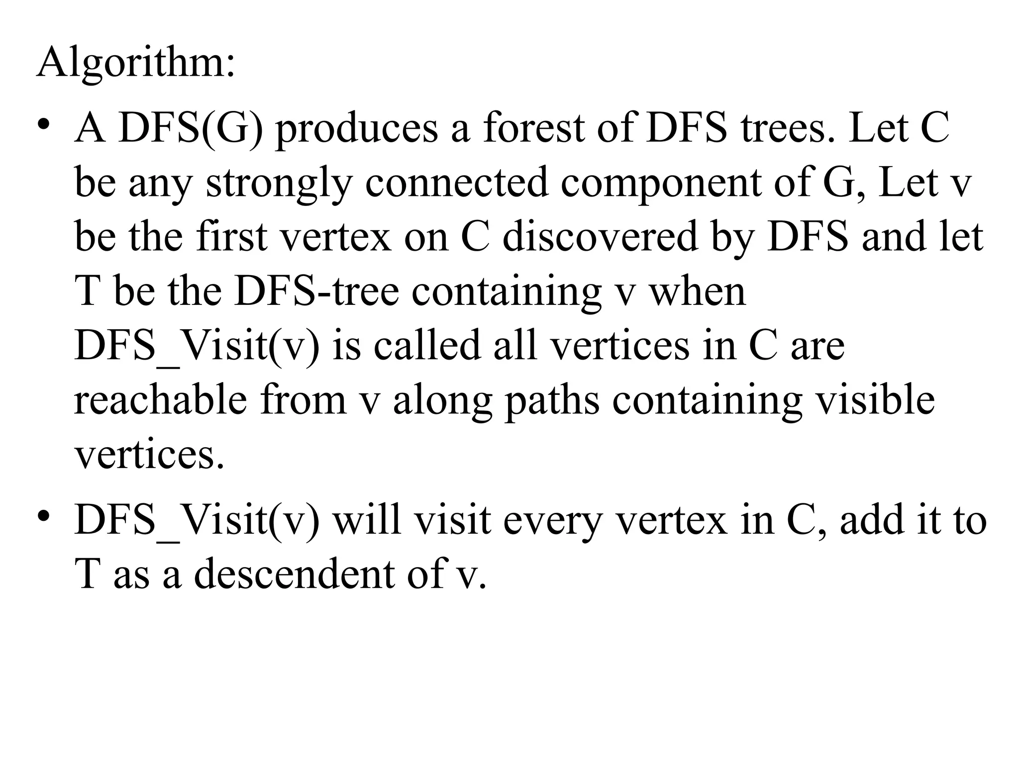
Algorithm:
• A DFS(G)produces a forest of DFS trees. Let C
be any strongly connected component of G, Let v
be the first vertex on C discovered by DFS and let
T be the DFS-tree containing v when
DFS_Visit(v) is called all vertices in C are
reachable from v along paths containing visible
vertices.
• DFS_Visit(v) will visit every vertex in C, add it to
T as a descendent of v.
79.
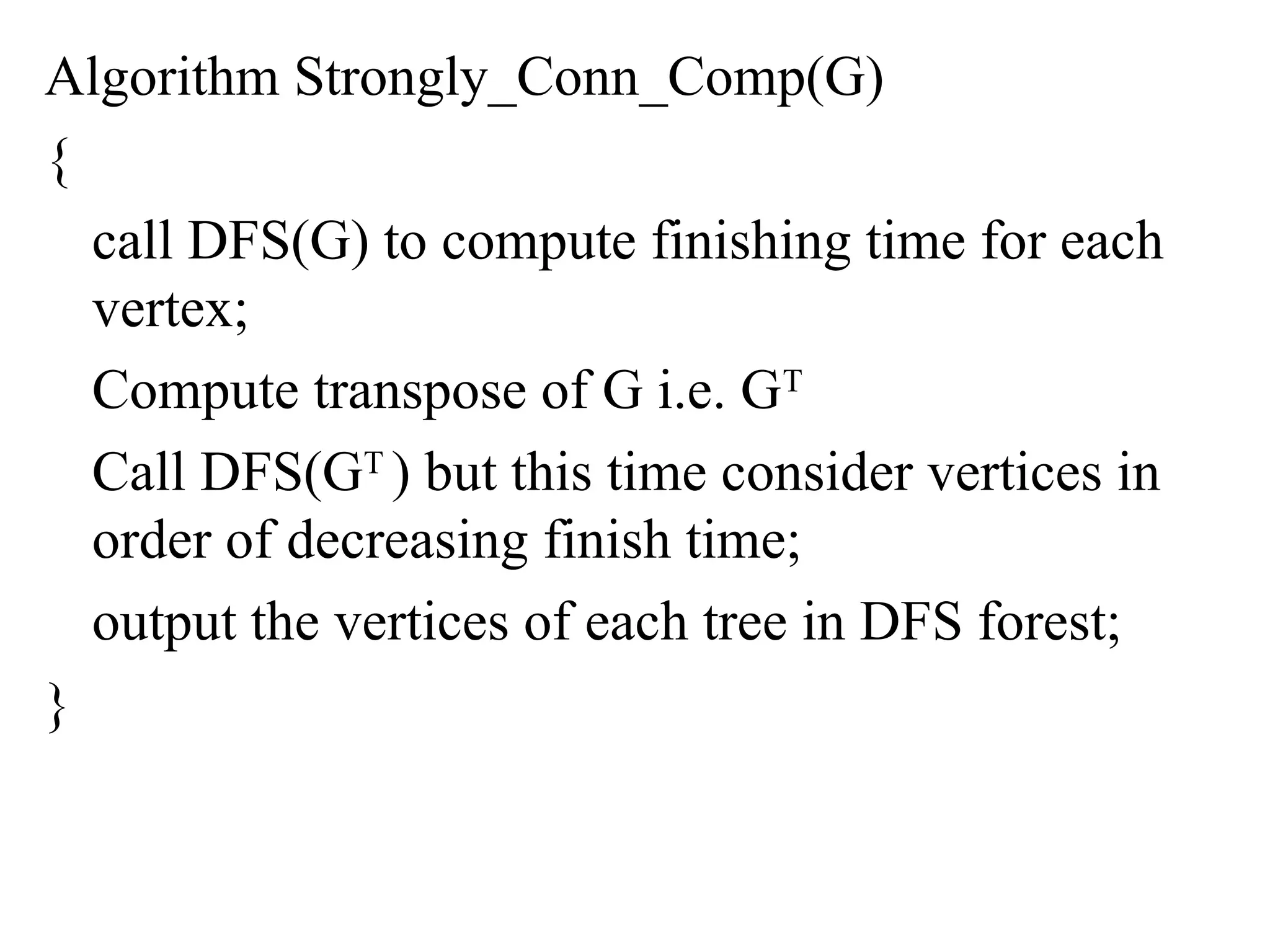
Algorithm Strongly_Conn_Comp(G)
{
call DFS(G)to compute finishing time for each
vertex;
Compute transpose of G i.e. GT
Call DFS(GT
) but this time consider vertices in
order of decreasing finish time;
output the vertices of each tree in DFS forest;
}
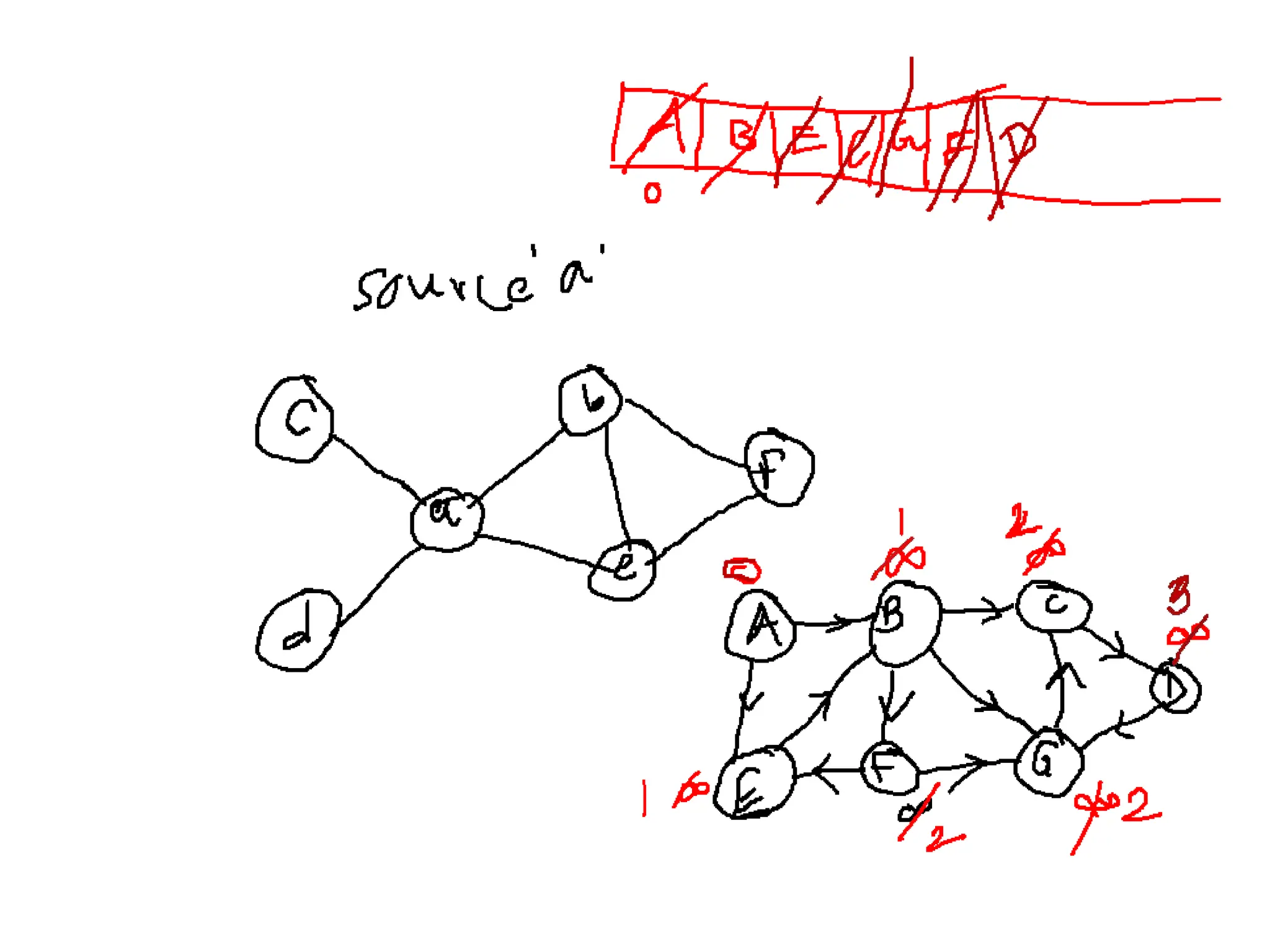
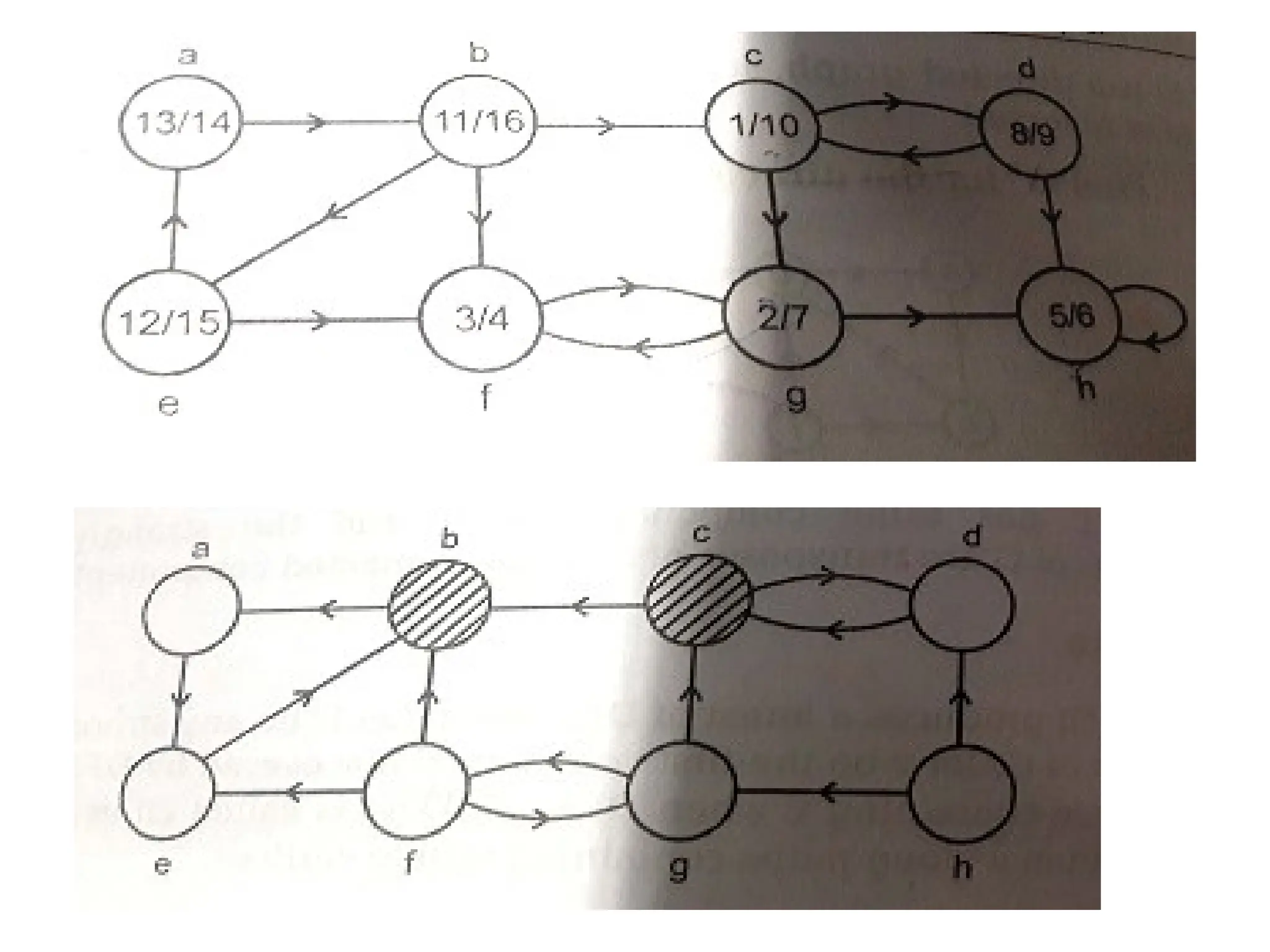
• Step1: callDFS(G) starting with the vertex c. For
each vertex inside node we write d[v]/f[v].
• Step2:compute GT
• Step3:Call DFS(GT
) but this time consider vertices
in order of decreasing finish time. First 16
i.e.vertex b-> component {a, b, e}
then start with 10 i.e.vertex c ->component {c, d}
then start with 7 i.e. vertex g->component {f, g}
the last component is{h}
• Step4: output the vertices of each tree in DFS
forest. {a, b, e}, {c, d},{f, g} and {h}
This algorithm has running time ɵ(V+E)

![Graph Representation
• Adjacency list representation of G = (V, E)
– An array of V lists, one for each vertex in V
– Each list Adj[u] contains all the vertices v such that
there is an edge between u and v
• Adj[u] contains the vertices adjacent to u (in arbitrary order)
– Can be used for both directed and undirected graphs
1 2
5 4
3
2 5 /
1 5 3 4 /
1
2
3
4
5
2 4
2 5 3 /
4 1 2
Undirected graph](https://image.slidesharecdn.com/chapter5decreaseconquer-251116093912-c4cb4eba/75/Design-and-analysis-of-algorithms-_-Decrease-and-Conquer-ppt-9-2048.jpg)
![• The breadth-first-search procedure BFS assumes that
the input graph G = (V,E) is represented using adjacency
lists.
• It maintains several additional data structures with each
vertex in the graph.
• The color of each vertex u ϵ V is stored in the variable
color[u], and the predecessor of u is stored in the
variable pi[u].
• If u has no predecessor (e.g. u is s or u has not been
discovered), then pi[u] = NIL.
• The distance from the source s to vertex u computed by
the algorithm is stored in d[u].
BFS(Breadth first search)
BFS(Breadth first search)](https://image.slidesharecdn.com/chapter5decreaseconquer-251116093912-c4cb4eba/75/Design-and-analysis-of-algorithms-_-Decrease-and-Conquer-ppt-19-2048.jpg)
![• The algorithm also uses a FIFO queue Q to
manage the set of gray vertices.
• BFS starts at a given vertex (Source), which is at
level 0.
• In first stage we will visit all vertices at level 1,all
white vertices which are adjacent to source.
• These are colored as grey and added to the
queue. Source is colored black.
• D[v] value of all these vertices is increased by 1.
(D[v] is distance of v from source.)
• Now visit all vertices at second level.
• Once vertex is explored it is colored black and is
deleted from queue.
• The process stops when queue is empty.](https://image.slidesharecdn.com/chapter5decreaseconquer-251116093912-c4cb4eba/75/Design-and-analysis-of-algorithms-_-Decrease-and-Conquer-ppt-20-2048.jpg)
![• Lines 1-4 paint every vertex white, set d[u] to be
infinity for each vertex u, and set the parent of
every vertex to be NIL.
• Line 5 paints the source vertex s gray, since it is
considered to be discovered when the procedure
begins.
• Line 6 initializes d[s] to be 0, and line 7 sets the
predecessor of the source to be NIL.
• Lines 8-9 initialize Q to the queue containing just
the vertex s.
Working of BFS
Working of BFS](https://image.slidesharecdn.com/chapter5decreaseconquer-251116093912-c4cb4eba/75/Design-and-analysis-of-algorithms-_-Decrease-and-Conquer-ppt-22-2048.jpg)


![• Besides creating a depth-first forest, DFS
also timestamps each vertex.
• Each vertex u has 2 timestamps: the first
timestamp d[u] records when u is first
discovered (and grayed), and the second
timestamp f[u] records when the search
finishes examining u’s adjacency list (and
blackens u).
• These timestamps are used in many graph
algorithms and are generally helpful in
reasoning about the behavior of DFS.](https://image.slidesharecdn.com/chapter5decreaseconquer-251116093912-c4cb4eba/75/Design-and-analysis-of-algorithms-_-Decrease-and-Conquer-ppt-59-2048.jpg)
![• Step1: call DFS(G) starting with the vertex c. For
each vertex inside node we write d[v]/f[v].
• Step2:compute GT
• Step3:Call DFS(GT
) but this time consider vertices
in order of decreasing finish time. First 16
i.e.vertex b-> component {a, b, e}
then start with 10 i.e.vertex c ->component {c, d}
then start with 7 i.e. vertex g->component {f, g}
the last component is{h}
• Step4: output the vertices of each tree in DFS
forest. {a, b, e}, {c, d},{f, g} and {h}
This algorithm has running time ɵ(V+E)](https://image.slidesharecdn.com/chapter5decreaseconquer-251116093912-c4cb4eba/75/Design-and-analysis-of-algorithms-_-Decrease-and-Conquer-ppt-81-2048.jpg)


![Graph Representation
• Adjacency list representation of G = (V, E)
– An array of V lists, one for each vertex in V
– Each list Adj[u] contains all the vertices v such that
there is an edge between u and v
• Adj[u] contains the vertices adjacent to u (in arbitrary order)
– Can be used for both directed and undirected graphs
1 2
5 4
3
2 5 /
1 5 3 4 /
1
2
3
4
5
2 4
2 5 3 /
4 1 2
Undirected graph](https://crownmelresort.com/image.slidesharecdn.com/chapter5decreaseconquer-251116093912-c4cb4eba/75/Design-and-analysis-of-algorithms-_-Decrease-and-Conquer-ppt-9-2048.jpg)


![• The breadth-first-search procedure BFS assumes that
the input graph G = (V,E) is represented using adjacency
lists.
• It maintains several additional data structures with each
vertex in the graph.
• The color of each vertex u ϵ V is stored in the variable
color[u], and the predecessor of u is stored in the
variable pi[u].
• If u has no predecessor (e.g. u is s or u has not been
discovered), then pi[u] = NIL.
• The distance from the source s to vertex u computed by
the algorithm is stored in d[u].
BFS(Breadth first search)
BFS(Breadth first search)](https://crownmelresort.com/image.slidesharecdn.com/chapter5decreaseconquer-251116093912-c4cb4eba/75/Design-and-analysis-of-algorithms-_-Decrease-and-Conquer-ppt-19-2048.jpg)
![• The algorithm also uses a FIFO queue Q to
manage the set of gray vertices.
• BFS starts at a given vertex (Source), which is at
level 0.
• In first stage we will visit all vertices at level 1,all
white vertices which are adjacent to source.
• These are colored as grey and added to the
queue. Source is colored black.
• D[v] value of all these vertices is increased by 1.
(D[v] is distance of v from source.)
• Now visit all vertices at second level.
• Once vertex is explored it is colored black and is
deleted from queue.
• The process stops when queue is empty.](https://crownmelresort.com/image.slidesharecdn.com/chapter5decreaseconquer-251116093912-c4cb4eba/75/Design-and-analysis-of-algorithms-_-Decrease-and-Conquer-ppt-20-2048.jpg)

![• Lines 1-4 paint every vertex white, set d[u] to be
infinity for each vertex u, and set the parent of
every vertex to be NIL.
• Line 5 paints the source vertex s gray, since it is
considered to be discovered when the procedure
begins.
• Line 6 initializes d[s] to be 0, and line 7 sets the
predecessor of the source to be NIL.
• Lines 8-9 initialize Q to the queue containing just
the vertex s.
Working of BFS
Working of BFS](https://crownmelresort.com/image.slidesharecdn.com/chapter5decreaseconquer-251116093912-c4cb4eba/75/Design-and-analysis-of-algorithms-_-Decrease-and-Conquer-ppt-22-2048.jpg)


![• Besides creating a depth-first forest, DFS
also timestamps each vertex.
• Each vertex u has 2 timestamps: the first
timestamp d[u] records when u is first
discovered (and grayed), and the second
timestamp f[u] records when the search
finishes examining u’s adjacency list (and
blackens u).
• These timestamps are used in many graph
algorithms and are generally helpful in
reasoning about the behavior of DFS.](https://crownmelresort.com/image.slidesharecdn.com/chapter5decreaseconquer-251116093912-c4cb4eba/75/Design-and-analysis-of-algorithms-_-Decrease-and-Conquer-ppt-59-2048.jpg)


![• Step1: call DFS(G) starting with the vertex c. For
each vertex inside node we write d[v]/f[v].
• Step2:compute GT
• Step3:Call DFS(GT
) but this time consider vertices
in order of decreasing finish time. First 16
i.e.vertex b-> component {a, b, e}
then start with 10 i.e.vertex c ->component {c, d}
then start with 7 i.e. vertex g->component {f, g}
the last component is{h}
• Step4: output the vertices of each tree in DFS
forest. {a, b, e}, {c, d},{f, g} and {h}
This algorithm has running time ɵ(V+E)](https://crownmelresort.com/image.slidesharecdn.com/chapter5decreaseconquer-251116093912-c4cb4eba/75/Design-and-analysis-of-algorithms-_-Decrease-and-Conquer-ppt-81-2048.jpg)


![Laminated_Springs[1]. Machine design practice](https://cdn.slidesharecdn.com/ss_thumbnails/laminatedsprings1-251116120255-2a3c06fb-thumbnail.jpg?width=640&height=640&fit=bounds)


