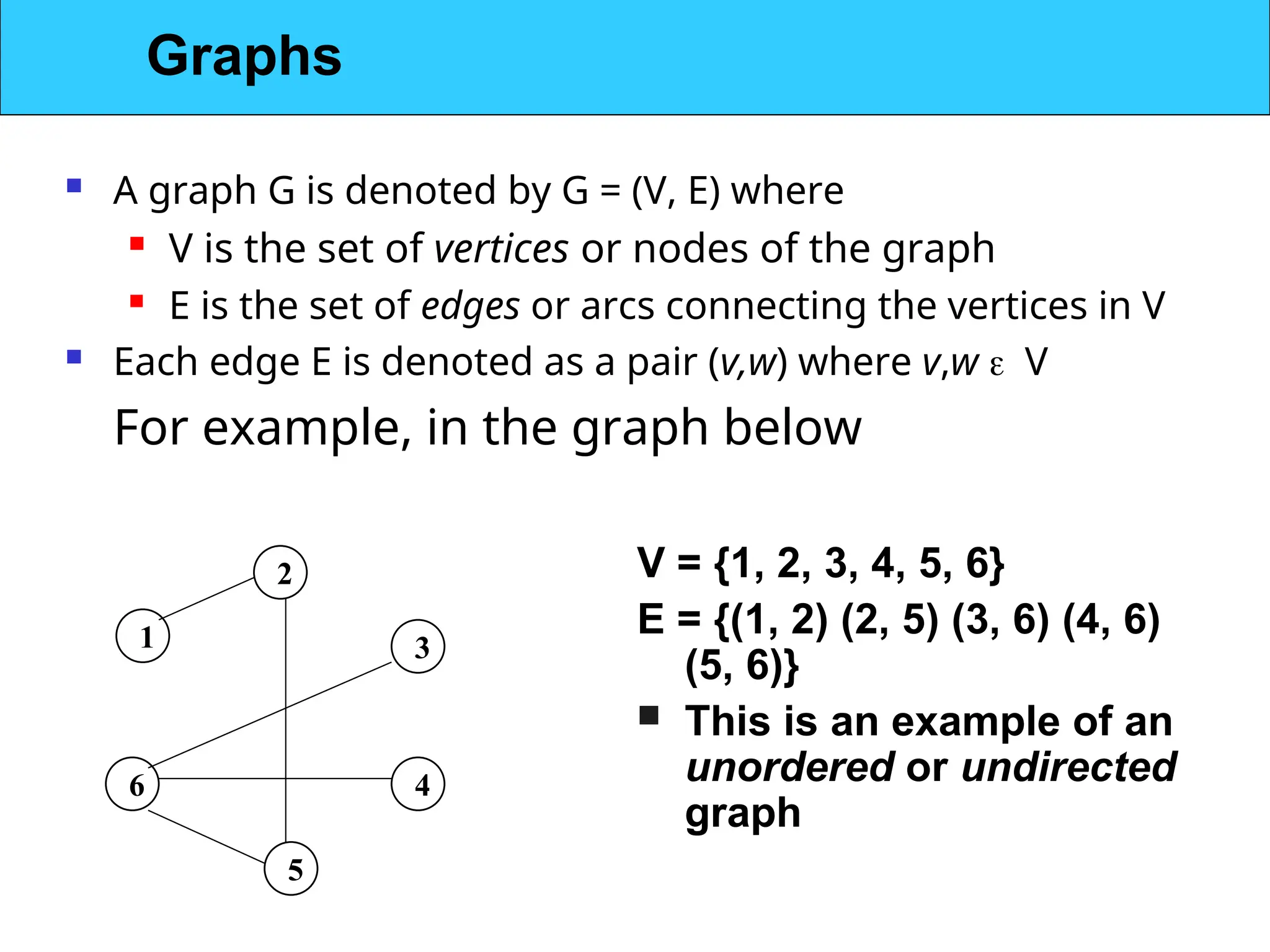
Graphs Presentation of University by Coordinator

 A graph G is denoted by G = (V, E) where
 V is the set of vertices or nodes of the graph
 E is the set of edges or arcs connecting the vertices in V
 Each edge E is denoted as a pair (v,w) where v,w V
For example, in the graph below
1
2
5
6 4
3
V = {1, 2, 3, 4, 5, 6}
E = {(1, 2) (2, 5) (3, 6) (4, 6)
(5, 6)}
 This is an example of an
unordered or undirected
graph
Graphs

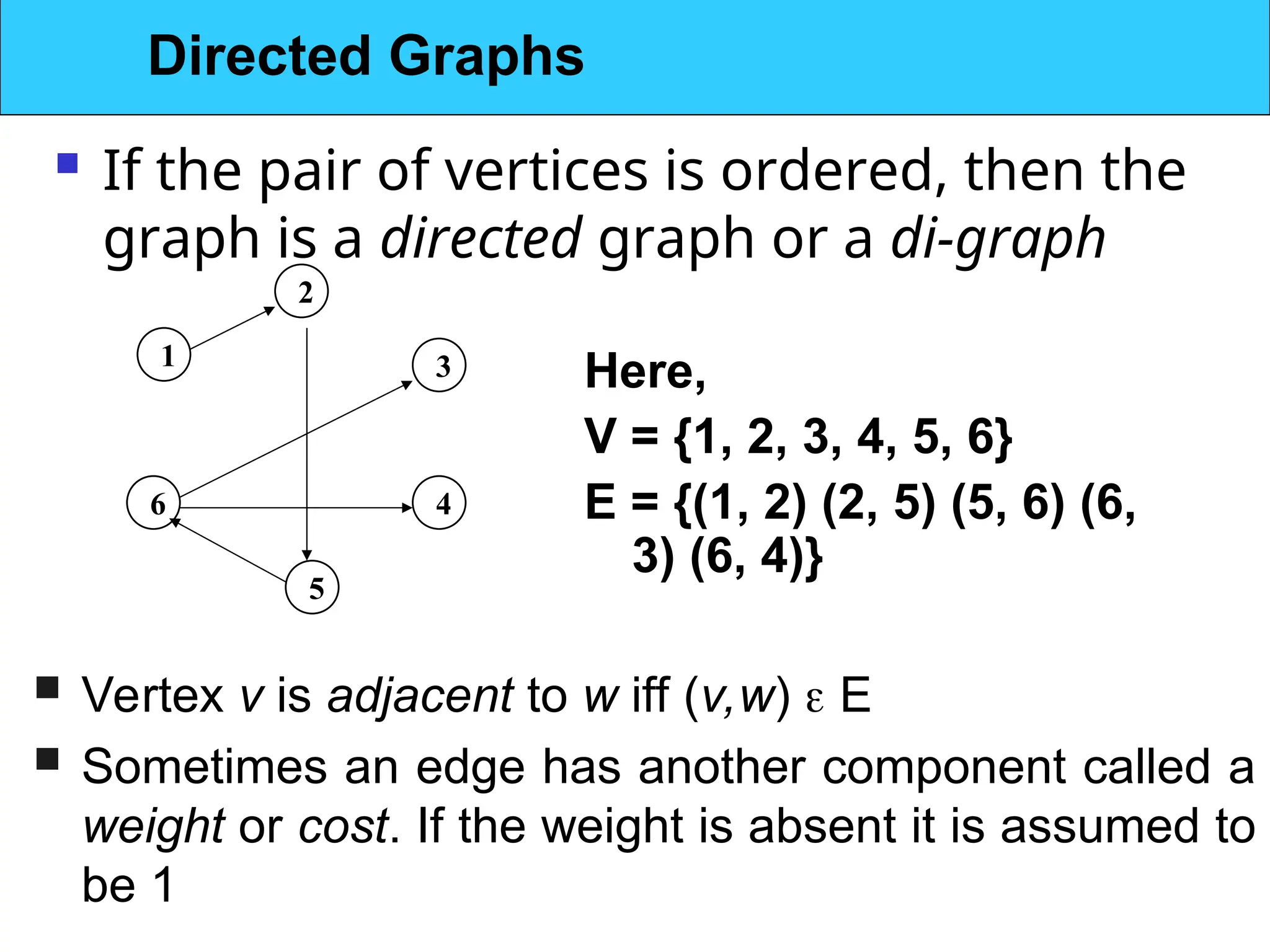
 If the pair of vertices is ordered, then the
graph is a directed graph or a di-graph
1
2
5
6 4
3 Here,
V = {1, 2, 3, 4, 5, 6}
E = {(1, 2) (2, 5) (5, 6) (6,
3) (6, 4)}
 Vertex v is adjacent to w iff (v,w)  E
 Sometimes an edge has another component called a
weight or cost. If the weight is absent it is assumed to
be 1
Directed Graphs

 A path is a sequence of vertices w1, w2, w3, ....wn
such that (wi, wi+1)  E
 Length of a path = # edges in the path
 A loop is an edge from a vertex onto itself. It is
denoted by (v, v)
 A simple path is a path where no vertices are
repeated along the path
 A cycle is a path with at least one edge such that
the first and last vertices are the same, i.e. w1 = wn
Graph Definitions: Path

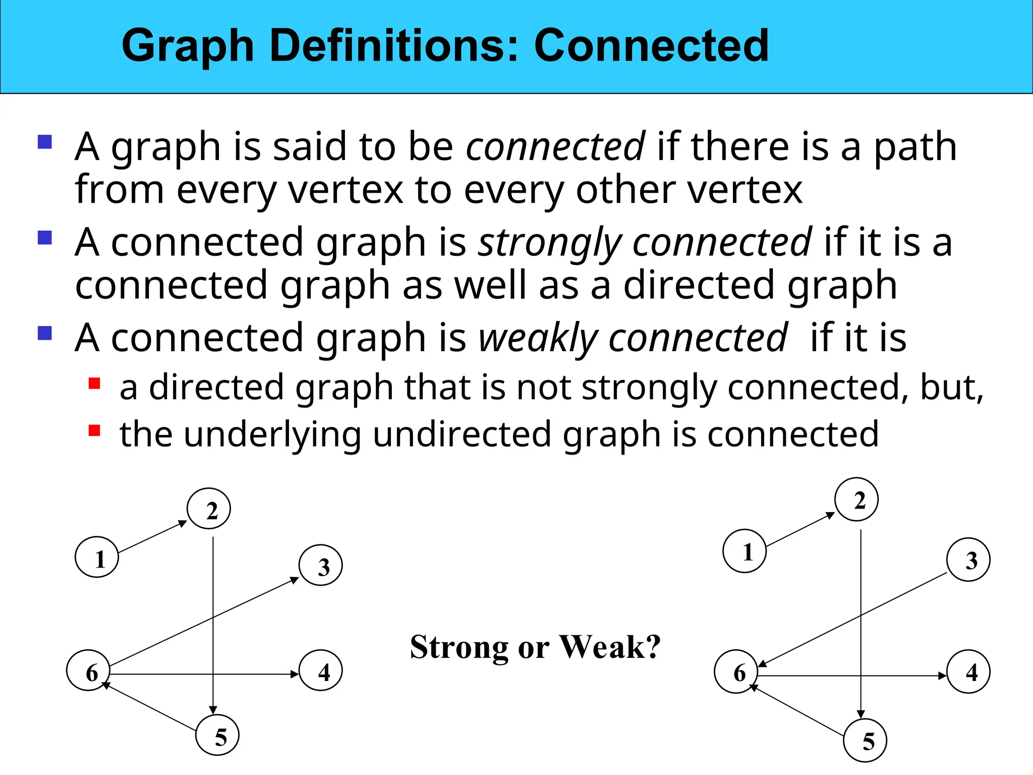
 A graph is said to be connected if there is a path
from every vertex to every other vertex
 A connected graph is strongly connected if it is a
connected graph as well as a directed graph
 A connected graph is weakly connected if it is
 a directed graph that is not strongly connected, but,
 the underlying undirected graph is connected
1
2
5
6 4
3
1
2
5
6 4
3
Strong or Weak?
Graph Definitions: Connected

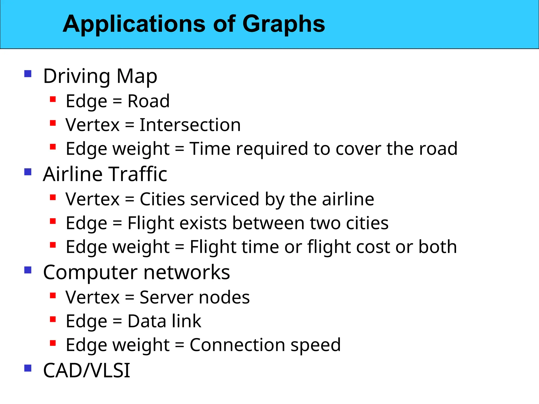
 Driving Map
 Edge = Road
 Vertex = Intersection
 Edge weight = Time required to cover the road
 Airline Traffic
 Vertex = Cities serviced by the airline
 Edge = Flight exists between two cities
 Edge weight = Flight time or flight cost or both
 Computer networks
 Vertex = Server nodes
 Edge = Data link
 Edge weight = Connection speed
 CAD/VLSI
Applications of Graphs

 Adjacency Matrix
 Two-dimensional matrix of size n x n where n is the
number of vertices in the graph
 a[i, j] = 0 if there is no edge between vertices i and j
 a[i, j] = 1 if there is an edge between vertices i and j
 Undirected graphs have both a[i, j] and a[j, i] = 1 if
there is an edge between vertices i and j
 a[i, j] = weight for weighted graphs
 Space requirement is (N2
)
 Problem: The array is very sparsely populated. For
example, if a directed graph has 4 vertices and 3
edges, the adjacency matrix has 16 cells only 3 of
which are 1
Representing Graphs: Adjacency Matrix

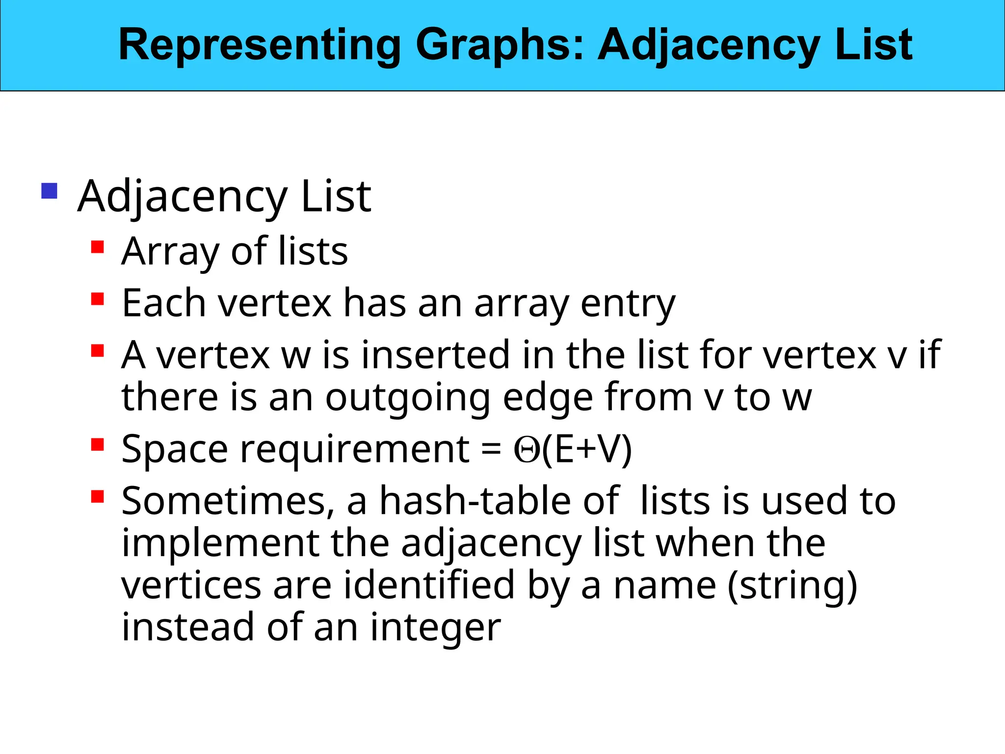
 Adjacency List
 Array of lists
 Each vertex has an array entry
 A vertex w is inserted in the list for vertex v if
there is an outgoing edge from v to w
 Space requirement = (E+V)
 Sometimes, a hash-table of lists is used to
implement the adjacency list when the
vertices are identified by a name (string)
instead of an integer
Representing Graphs: Adjacency List

1
2
5
6 4
3
1
2
3
4
5
6
2
5
6
4
3
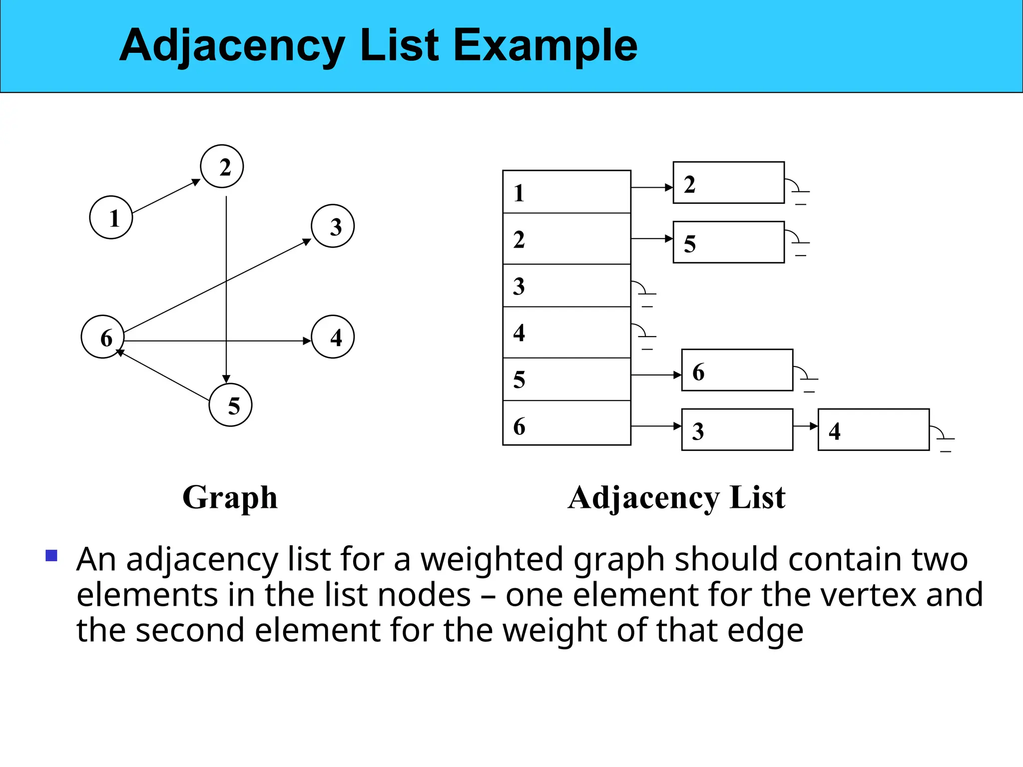
Graph Adjacency List
 An adjacency list for a weighted graph should contain two
elements in the list nodes – one element for the vertex and
the second element for the weight of that edge
Adjacency List Example

 Given: a graph G = (V, E), directed or
undirected
 Goal: methodically explore every vertex
and every edge
 Ultimately: build a tree on the graph
 Pick a vertex as the root

Choose certain edges to produce a tree

Note: might also build a forest if graph is not
connected
Graph Searching

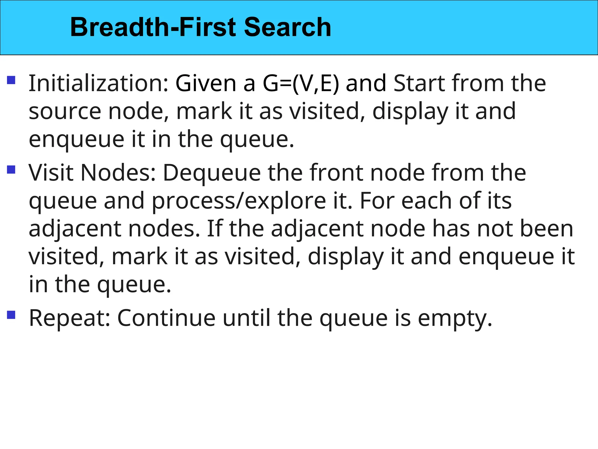
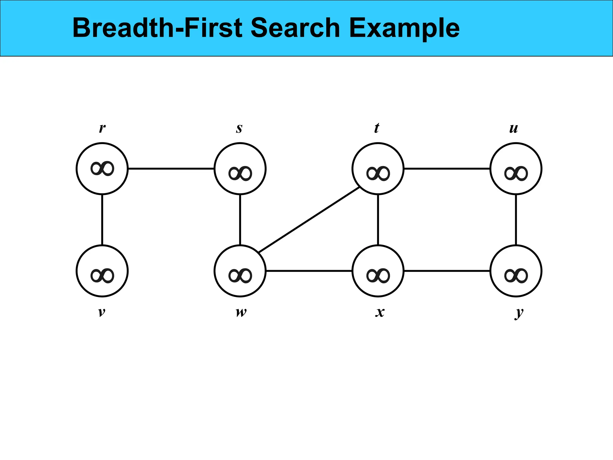
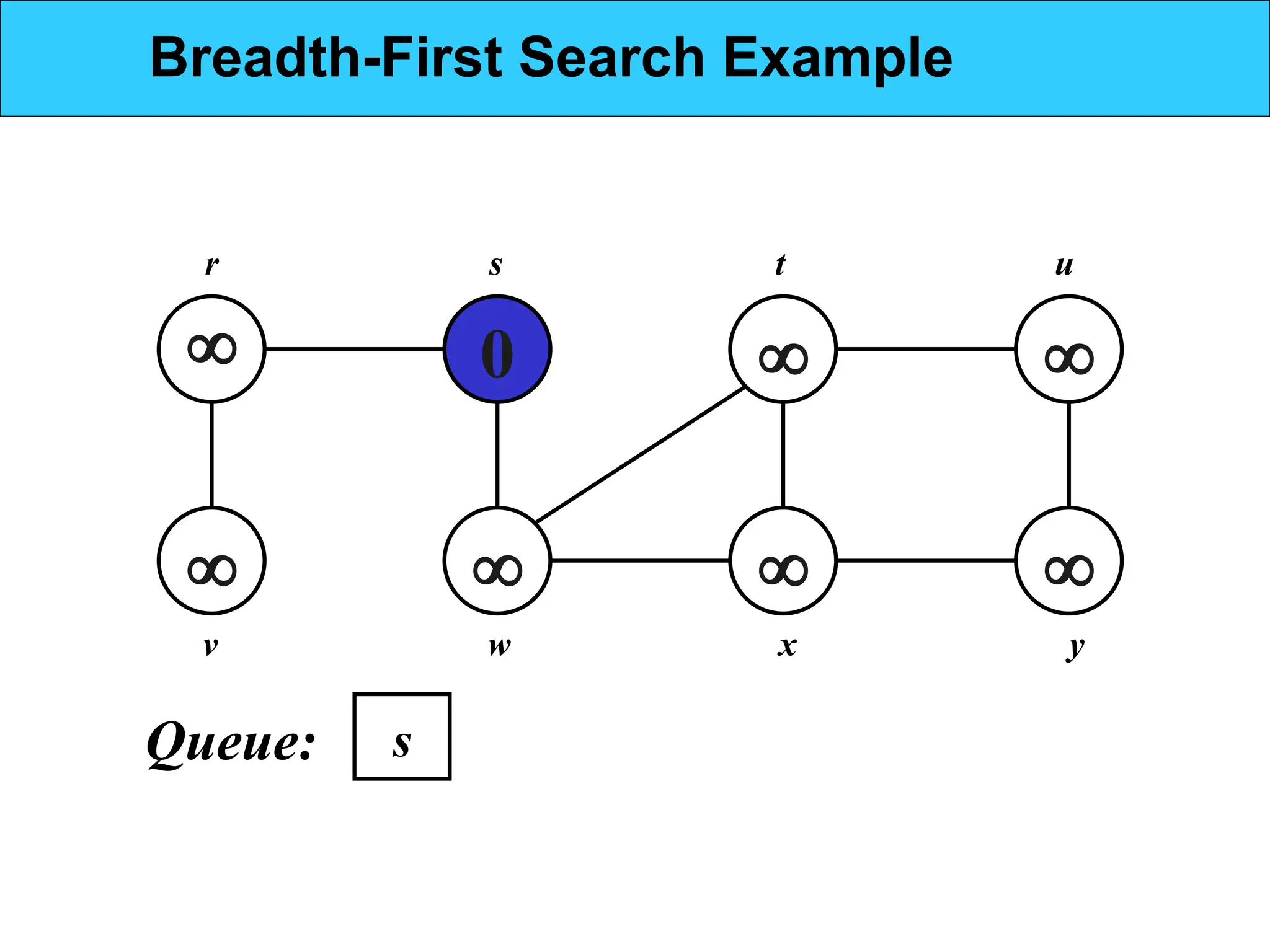
 Initialization: Given a G=(V,E) and Start from the
source node, mark it as visited, display it and
enqueue it in the queue.
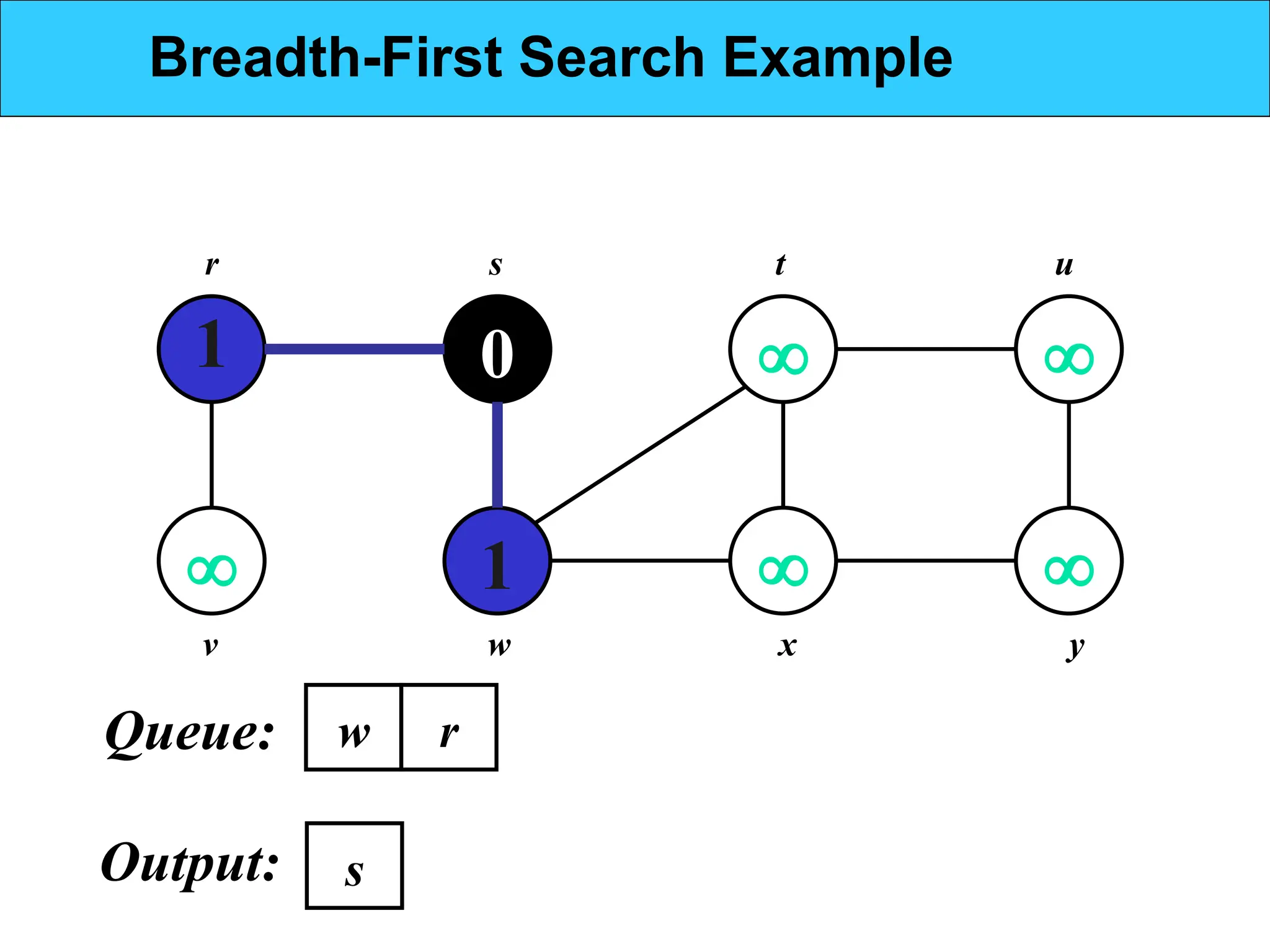
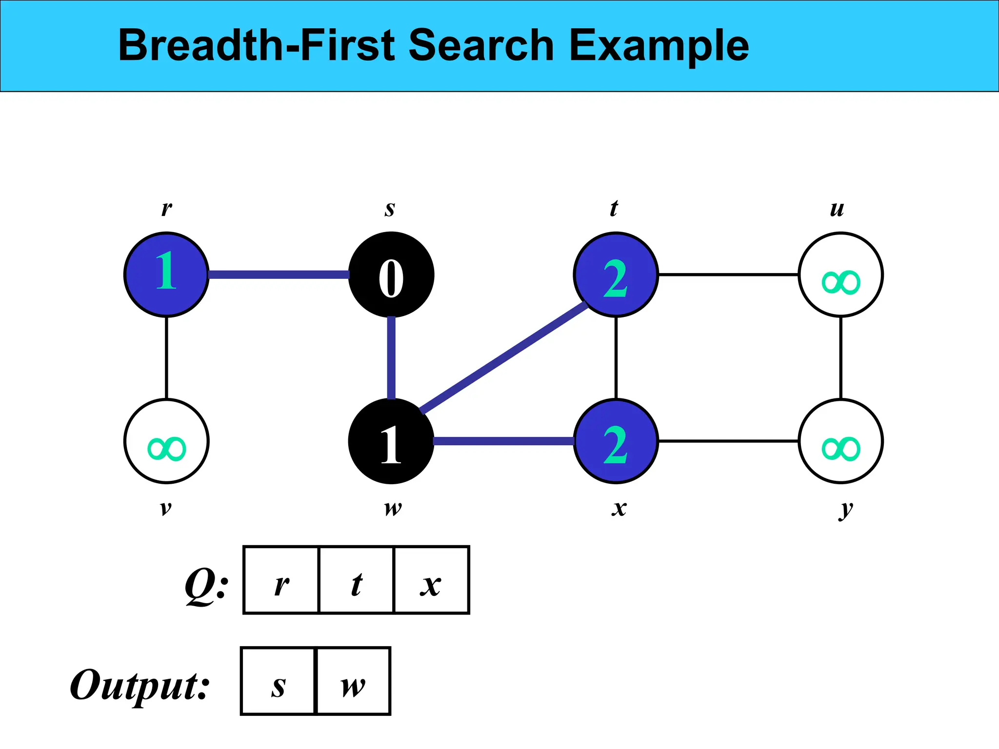
 Visit Nodes: Dequeue the front node from the
queue and process/explore it. For each of its
adjacent nodes. If the adjacent node has not been
visited, mark it as visited, display it and enqueue it
in the queue.
 Repeat: Continue until the queue is empty.
Breadth-First Search

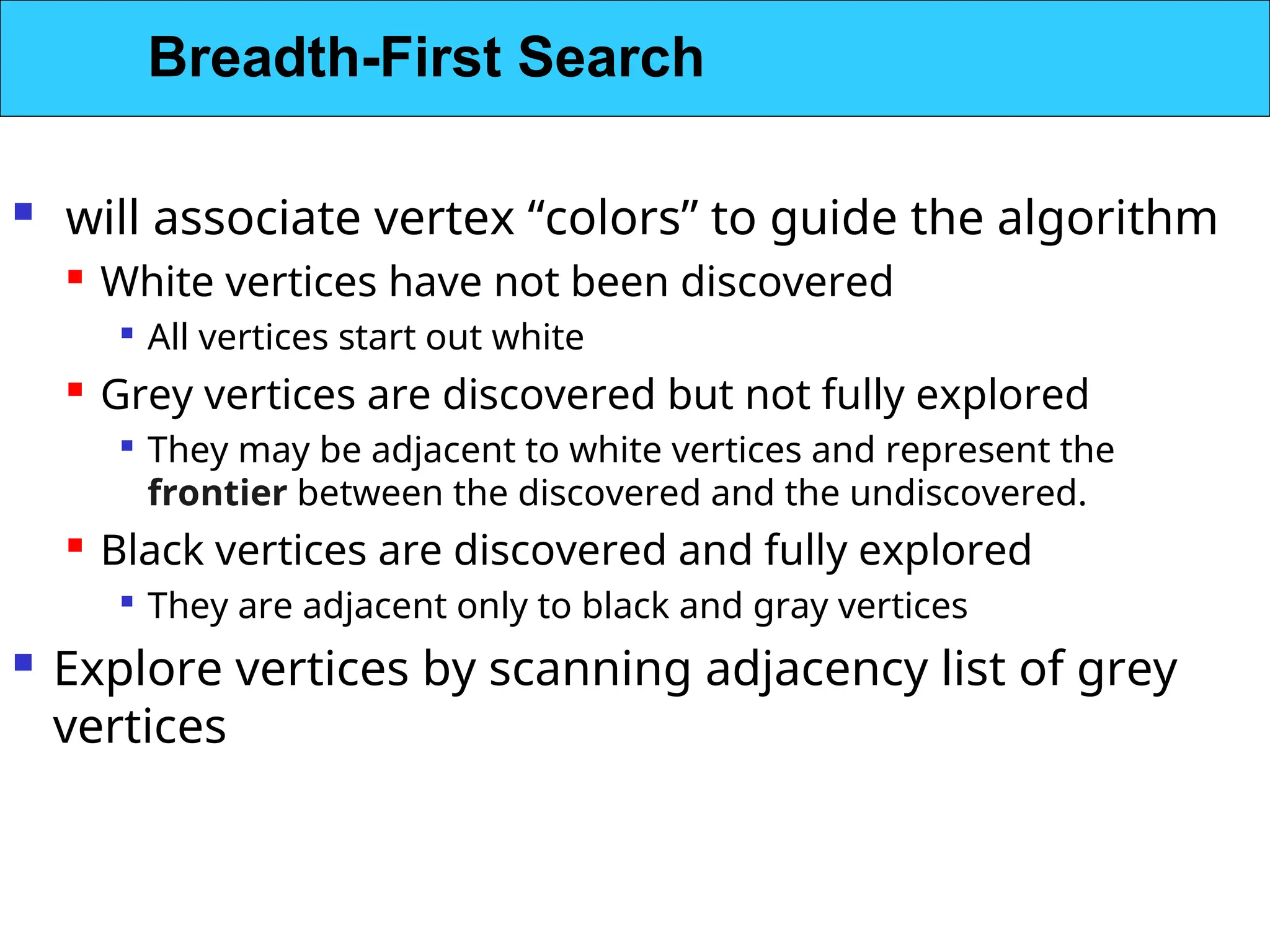
 will associate vertex “colors” to guide the algorithm

White vertices have not been discovered

All vertices start out white

Grey vertices are discovered but not fully explored

They may be adjacent to white vertices and represent the
frontier between the discovered and the undiscovered.
 Black vertices are discovered and fully explored

They are adjacent only to black and gray vertices
 Explore vertices by scanning adjacency list of grey
vertices
Breadth-First Search

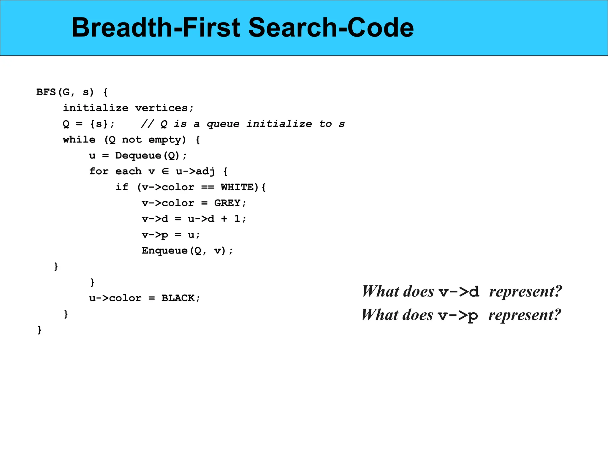
BFS(G, s) {
initialize vertices;
Q = {s}; // Q is a queue initialize to s
while (Q not empty) {
u = Dequeue(Q);
for each v  u->adj {
if (v->color == WHITE){
v->color = GREY;
v->d = u->d + 1;
v->p = u;
Enqueue(Q, v);
}
}
u->color = BLACK;
}
}
What does v->p represent?
What does v->d represent?
Breadth-First Search-Code









r s t u
v w x y
Breadth-First Search Example



0





r s t u
v w x y
s
Queue:

1

0
1




r s t u
v w x y
w r
s
Output:
Queue:

1

0
1
2
2


r s t u
v w x y
r
Q: t x
w
s
Output:

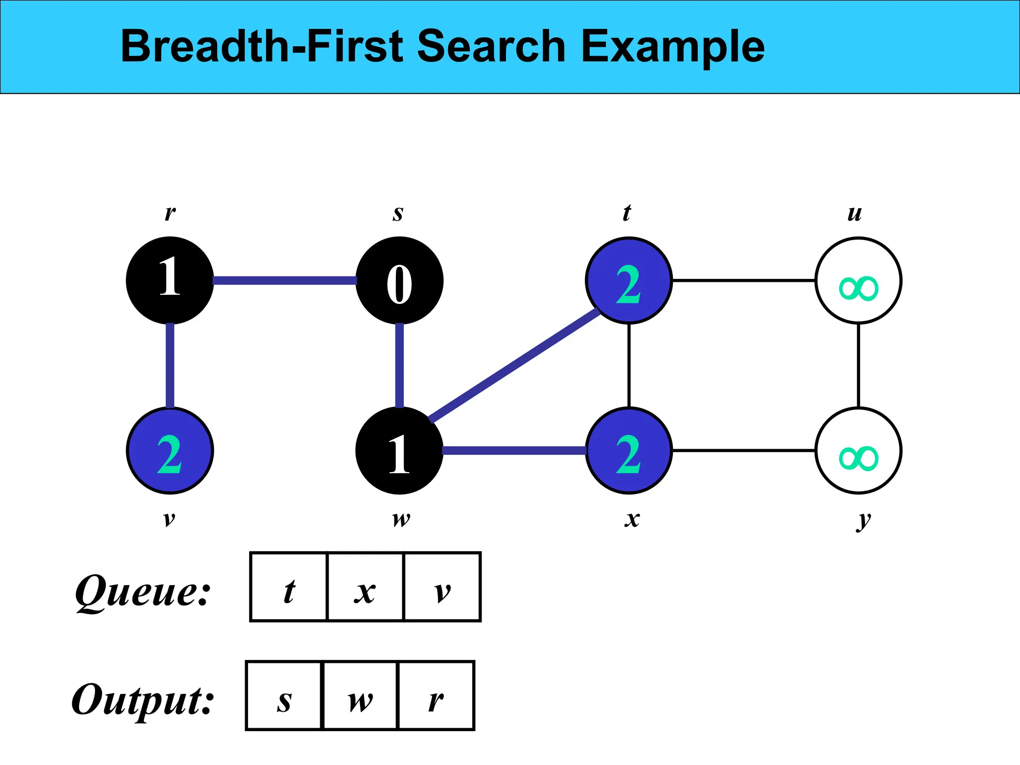
1
2
0
1
2
2


r s t u
v w x y
w
s
Output:
t x v
r
Queue:

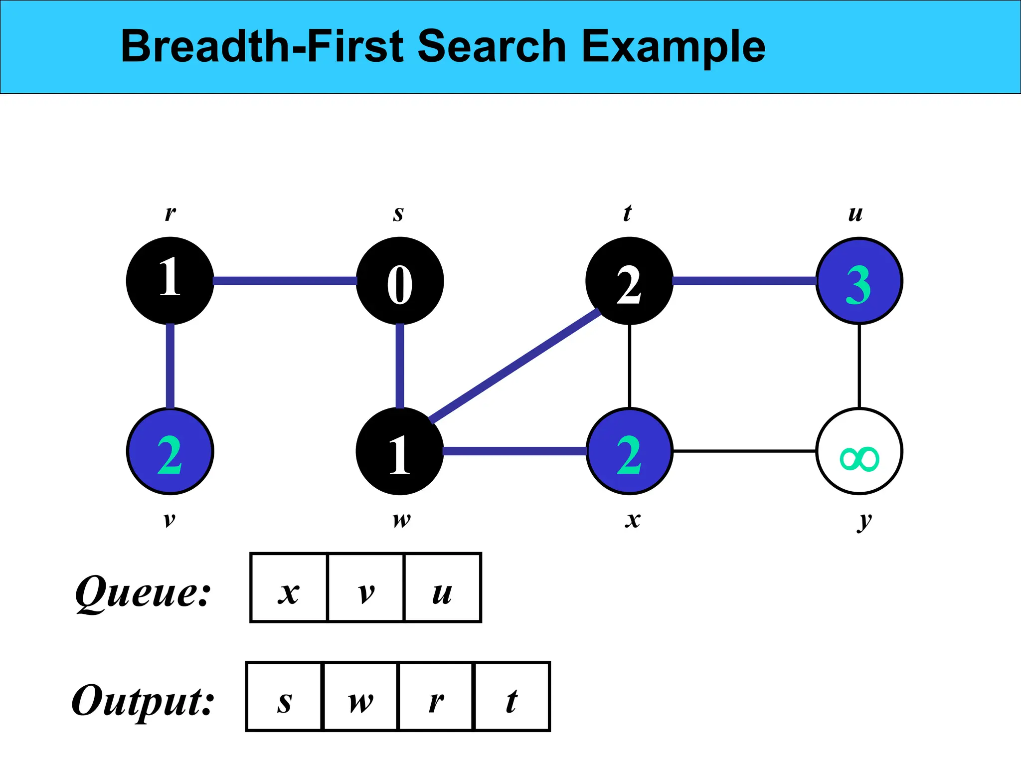
1
2
0
1
2
2
3

r s t u
v w x y
w
s
Output:
x v u
r
Queue:
t

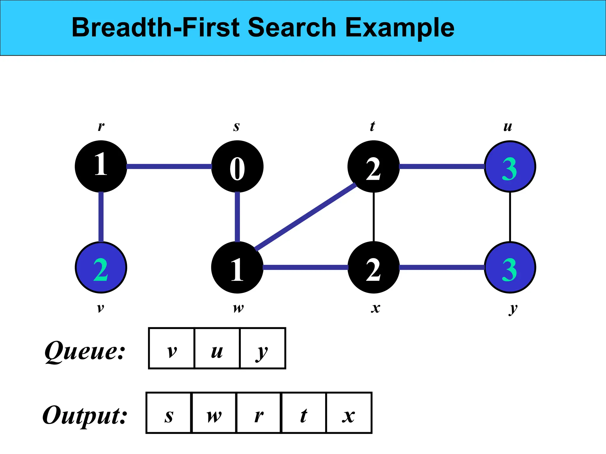
1
2
0
1
2
2
3
3
r s t u
v w x y
w
s
Output:
v u y
r
Queue:
t x

1
2
0
1
2
2
3
3
r s t u
v w x y
w
s
Output:
u y
r
Queue:
t x v

1
2
0
1
2
2
3
3
r s t u
v w x y
w
s
Output: u
y
r
Queue:
t x v

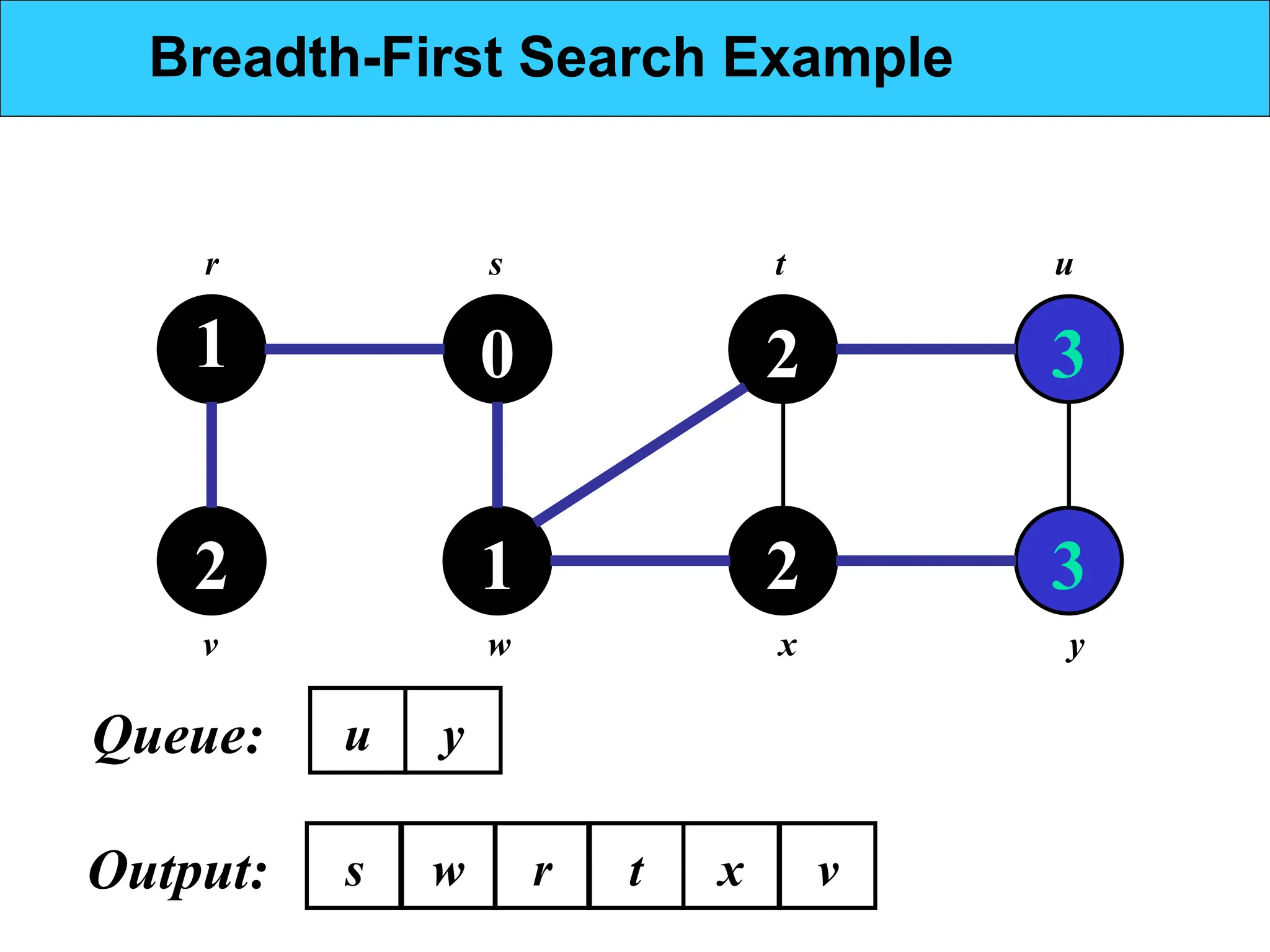
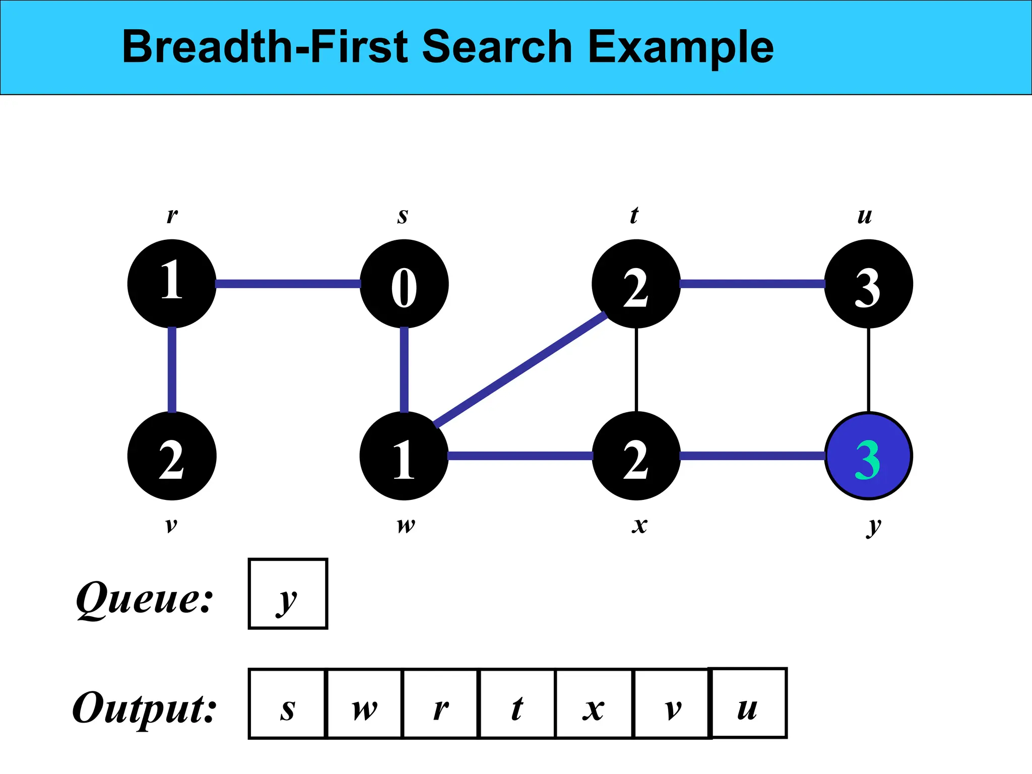
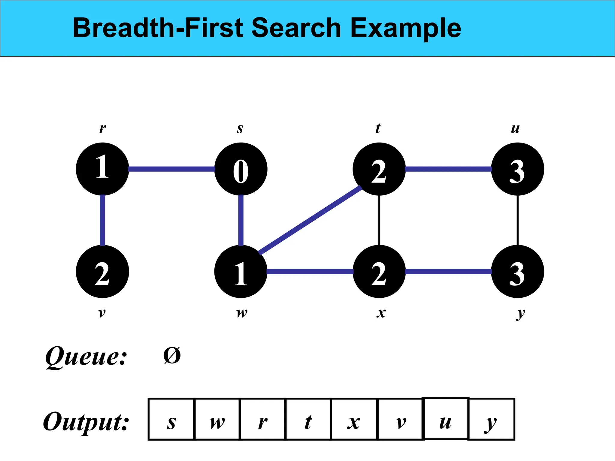
1
2
0
1
2
2
3
3
r s t u
v w x y
Ø
w
s
Output: u
r t x v
Queue:
y

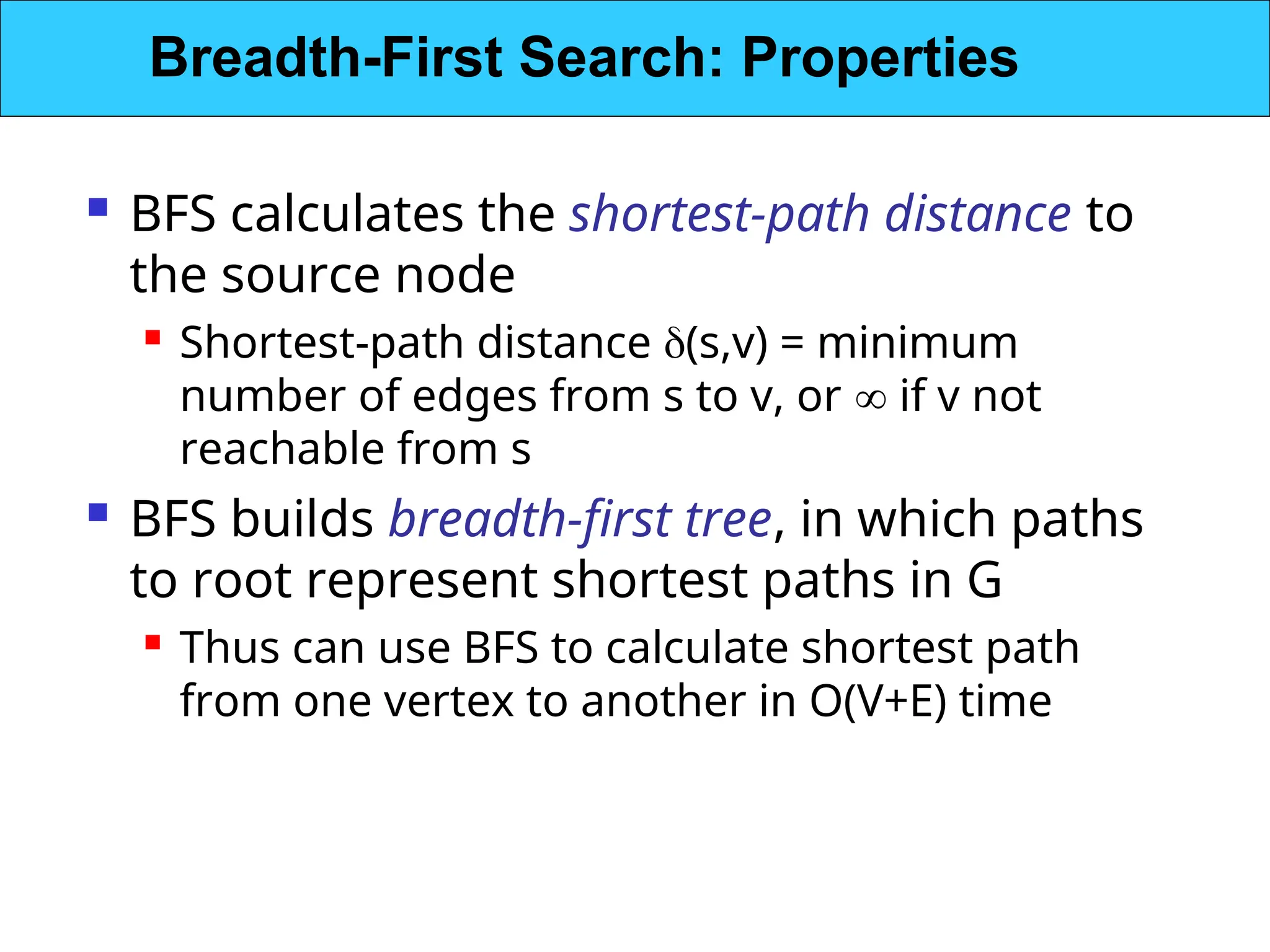
 BFS calculates the shortest-path distance to
the source node
 Shortest-path distance (s,v) = minimum
number of edges from s to v, or  if v not
reachable from s
 BFS builds breadth-first tree, in which paths
to root represent shortest paths in G
 Thus can use BFS to calculate shortest path
from one vertex to another in O(V+E) time
Breadth-First Search: Properties

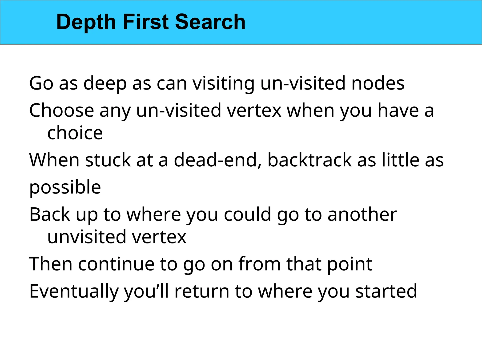
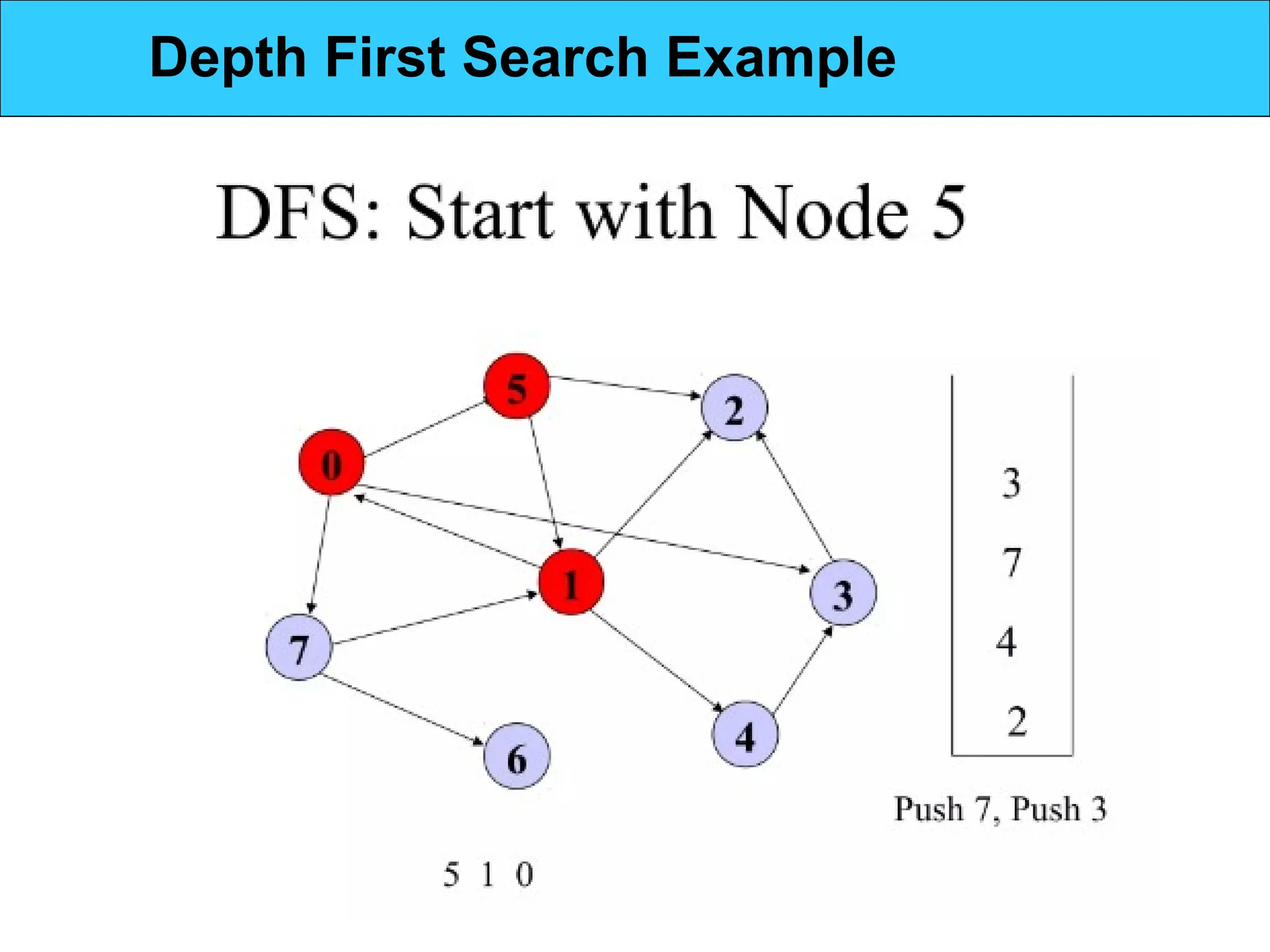
Go as deep as can visiting un-visited nodes
Choose any un-visited vertex when you have a
choice
When stuck at a dead-end, backtrack as little as
possible
Back up to where you could go to another
unvisited vertex
Then continue to go on from that point
Eventually you’ll return to where you started
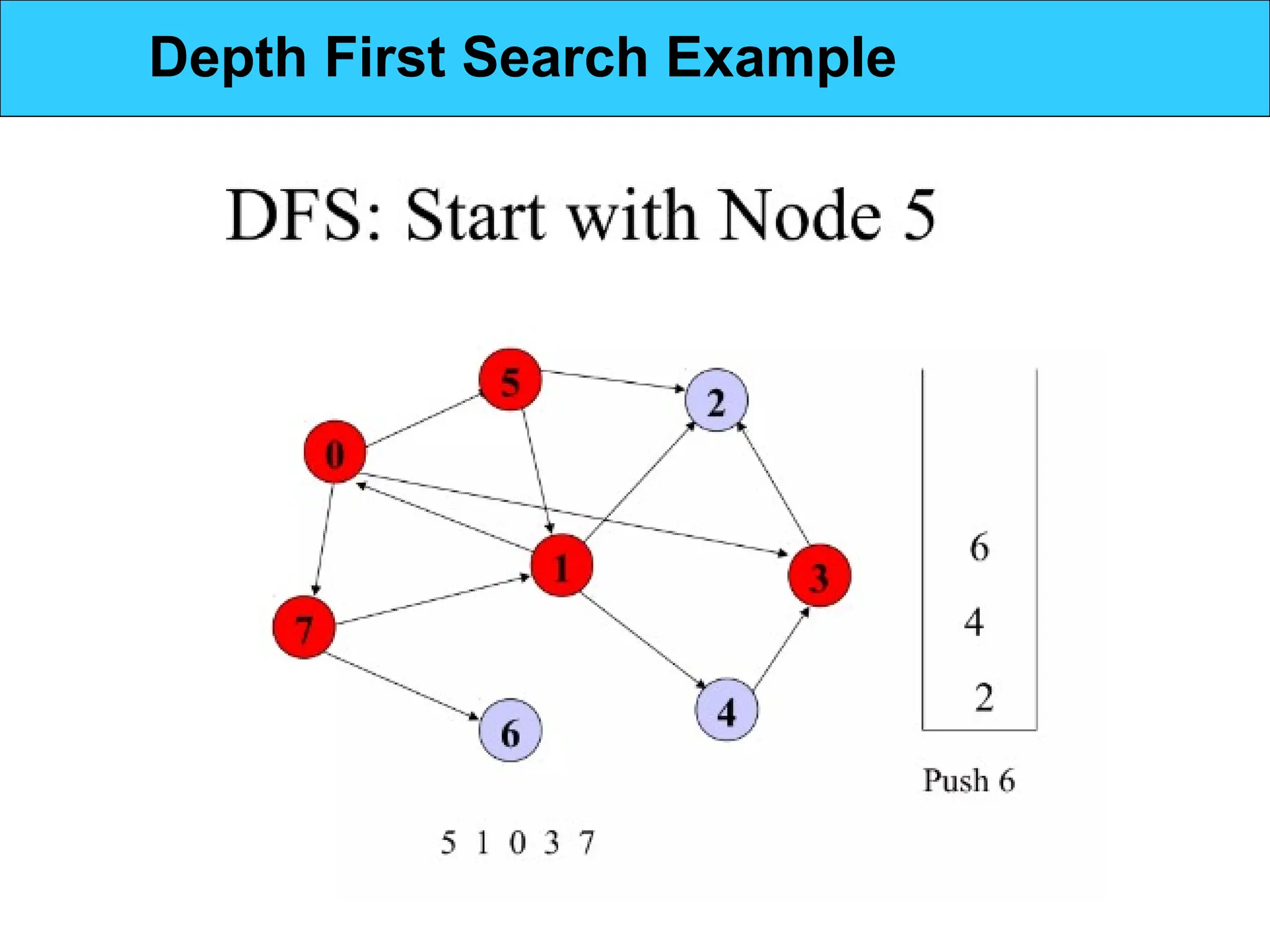
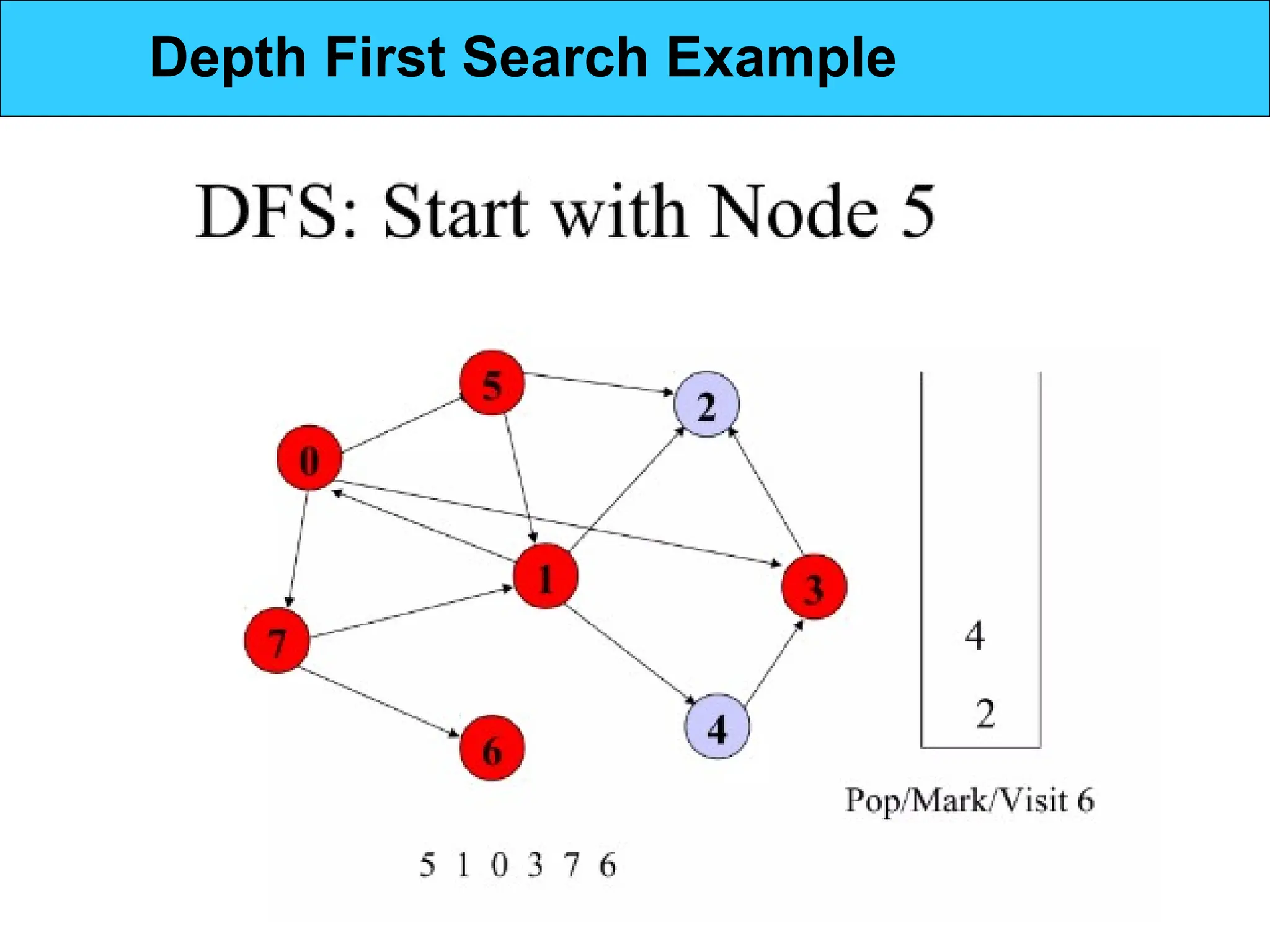
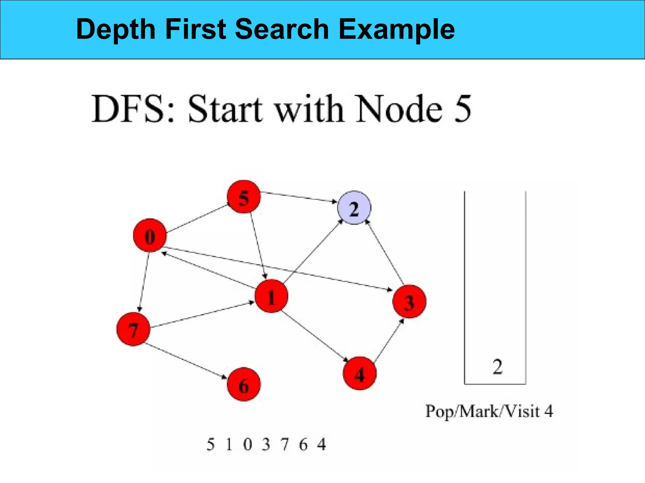
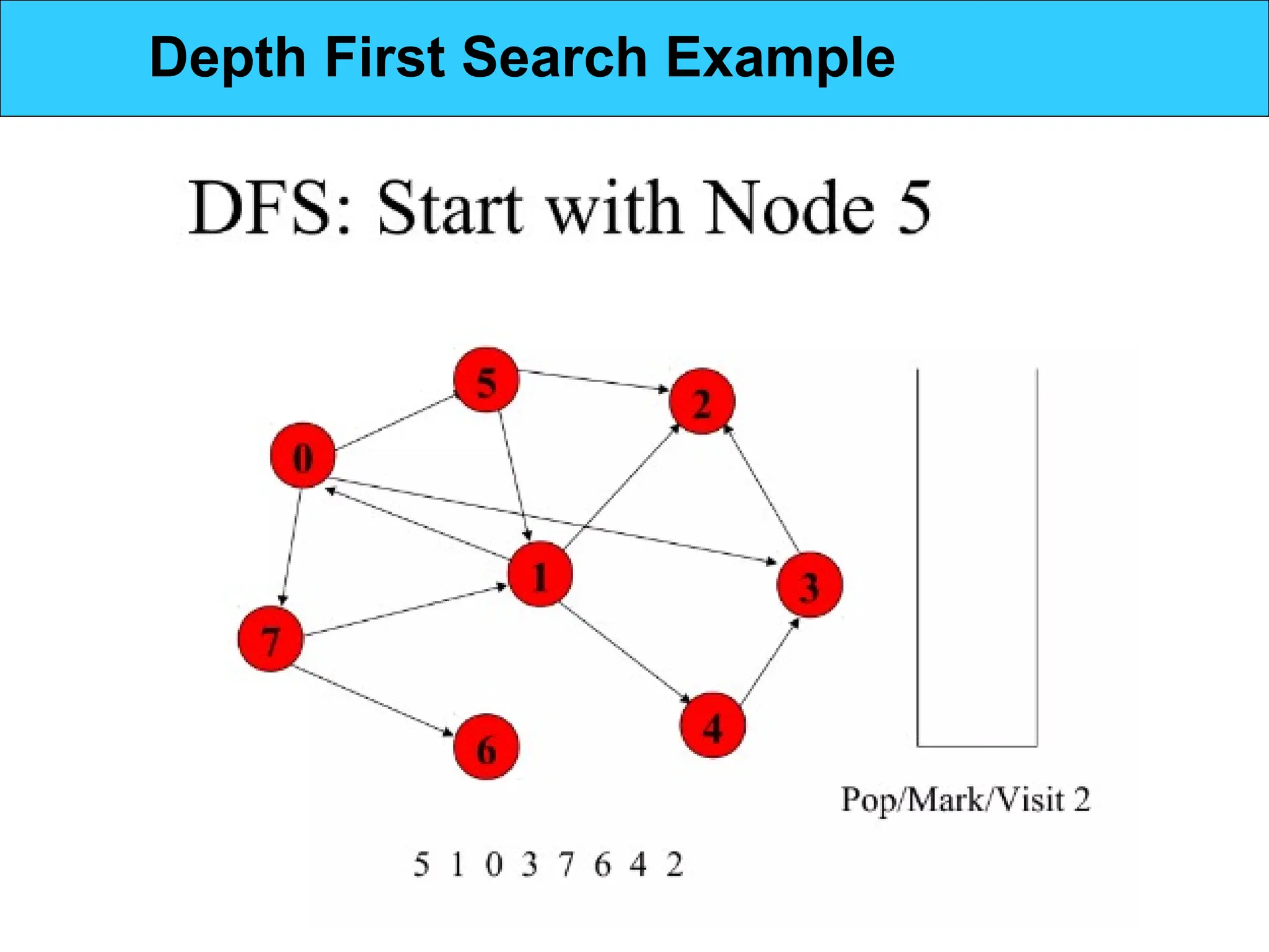
Depth First Search

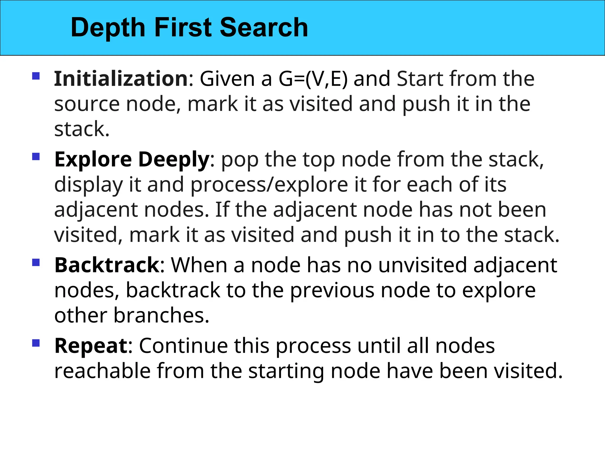
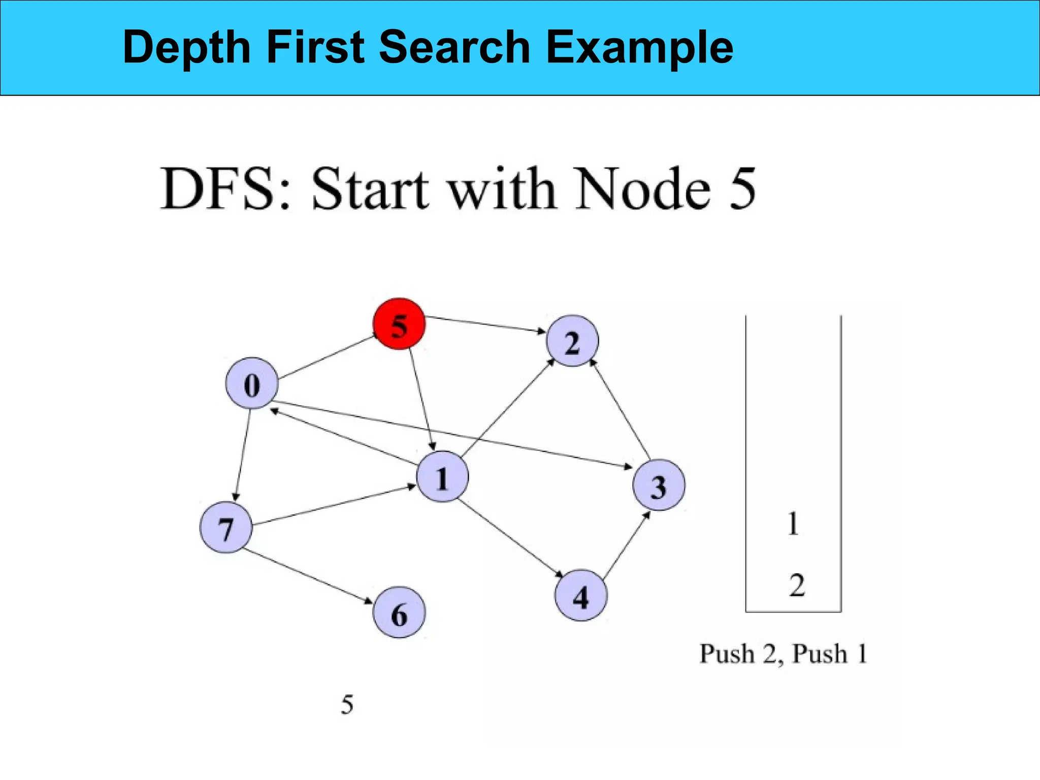
 Initialization: Given a G=(V,E) and Start from the
source node, mark it as visited and push it in the
stack.
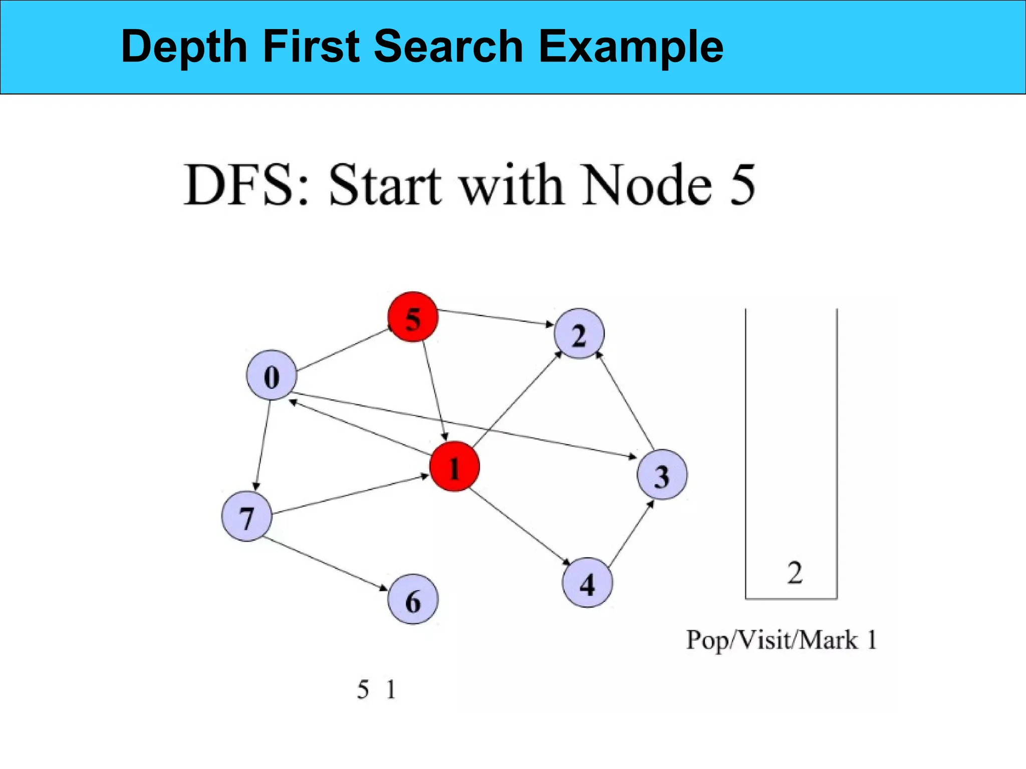
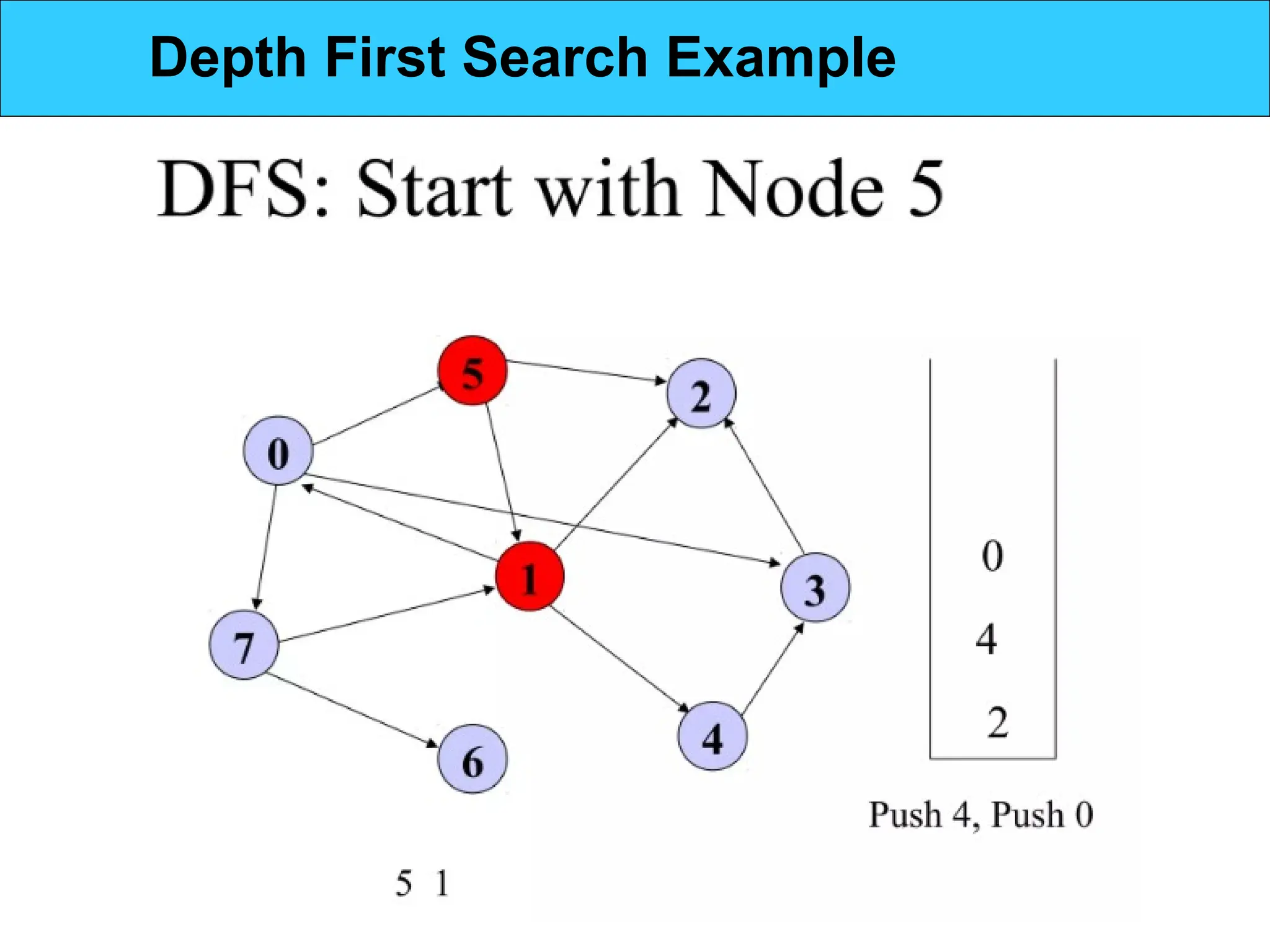
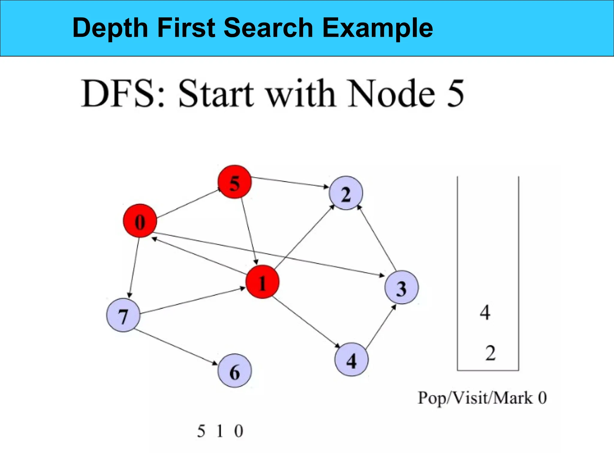
 Explore Deeply: pop the top node from the stack,
display it and process/explore it for each of its
adjacent nodes. If the adjacent node has not been
visited, mark it as visited and push it in to the stack.
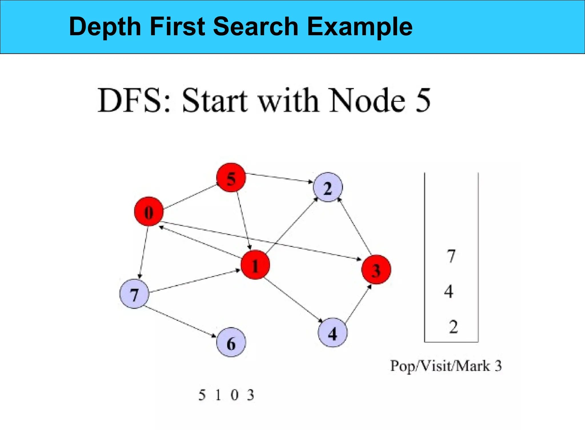
 Backtrack: When a node has no unvisited adjacent
nodes, backtrack to the previous node to explore
other branches.
 Repeat: Continue this process until all nodes
reachable from the starting node have been visited.
Depth First Search

DFS(G)
for each vertex u V[G] {
color[u]=white
parent[u]=NULL
}
time=0
for each vertex u V[G] {
if color[u]=white then
DFS-VISIT(u)
}
DFS Algorithm

DFS-VISIT(u)
color[u]=GRAY
time=time+1
d[u]=time
for each vertex v  adj[u] {
if color[v]=white Then
parent[v]=u
DFS-VISIT(v)
}
color[u]=black
f[u]=time=time+1
DFS Algorithm

Graphs Presentation of University by Coordinator

More Related Content

Similar to Graphs Presentation of University by Coordinator

More from haseebanjum2611

Recently uploaded

Graphs Presentation of University by Coordinator

Editor's Notes