Downloaded 19 times
![Graph Terminology:
• Node
Each element of a graph is called node of a graph
• Edge
Line joining two nodes is called an edge.
It is denoted by e=[u,v] where u and v are adjacent vertices.
6
Loop
An edge of the form (u, u) is said to be a loop. Here in figure [v2,v2]
Multiedge
If x was y’s friend several times over, we can model this relationship
using multiedges. In figure e1 and e3.
Loop
e1
V1
V2e2V2
node
edge
e3](https://image.slidesharecdn.com/unit-ixgraph-150919102535-lva1-app6892/75/Unit-ix-graph-6-2048.jpg)
![20
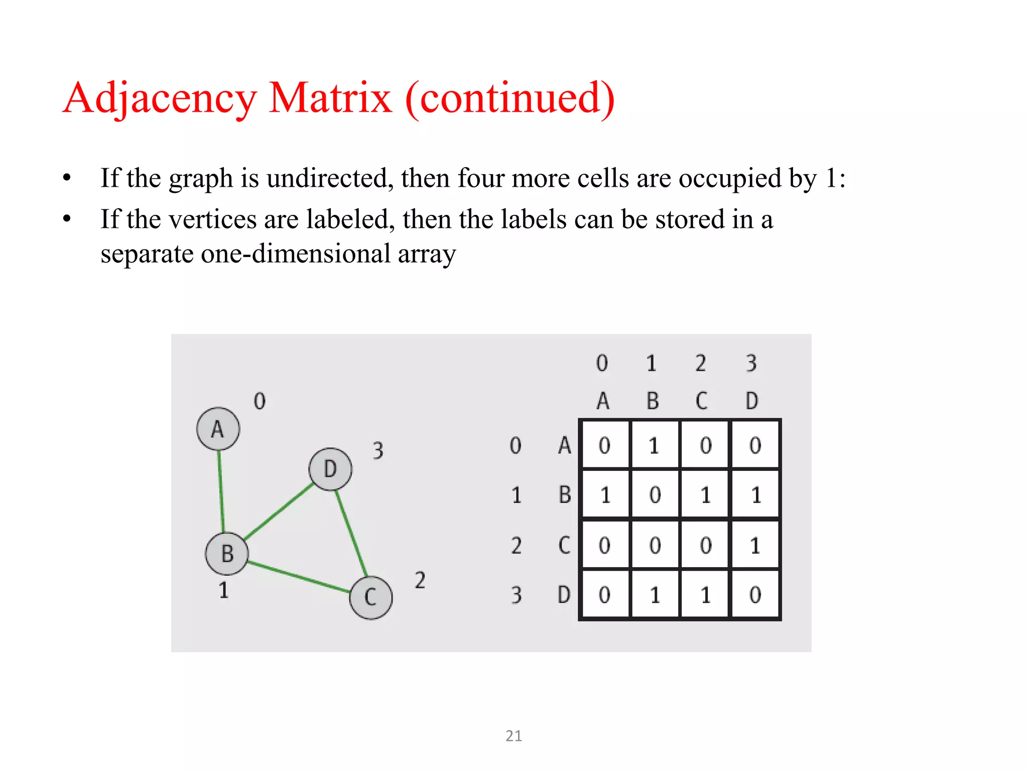
Adjacency Matrix
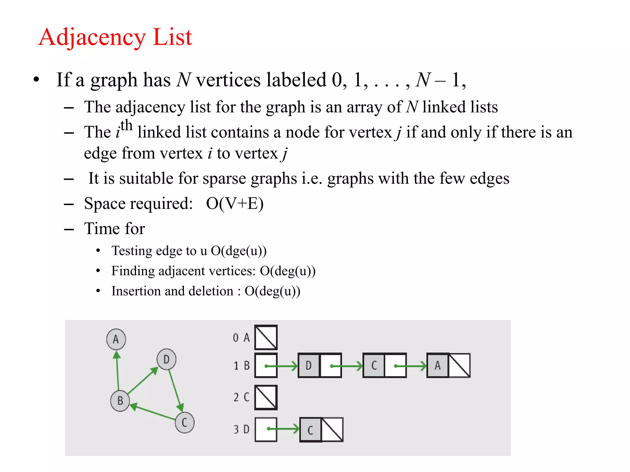
• If a graph has N vertices labeled 0, 1, . . . , N – 1:
– The adjacency matrix for the graph is a grid G with N rows and N columns
– Cell G[i][ j] = 1 if there’s an edge from vertex i to j
• Otherwise, there is no edge and that cell contains 0
• These are the simplest ways for representing graphs.
• Space requirement: O(n2)
• Adding and deleting edge: O(1)
• Testing an edge : O(1)](https://image.slidesharecdn.com/unit-ixgraph-150919102535-lva1-app6892/75/Unit-ix-graph-20-2048.jpg)


![Graph Terminology:
• Node
Each element of a graph is called node of a graph
• Edge
Line joining two nodes is called an edge.
It is denoted by e=[u,v] where u and v are adjacent vertices.
6
Loop
An edge of the form (u, u) is said to be a loop. Here in figure [v2,v2]
Multiedge
If x was y’s friend several times over, we can model this relationship
using multiedges. In figure e1 and e3.
Loop
e1
V1
V2e2V2
node
edge
e3](https://crownmelresort.com/image.slidesharecdn.com/unit-ixgraph-150919102535-lva1-app6892/75/Unit-ix-graph-6-2048.jpg)


![20
Adjacency Matrix
• If a graph has N vertices labeled 0, 1, . . . , N – 1:
– The adjacency matrix for the graph is a grid G with N rows and N columns
– Cell G[i][ j] = 1 if there’s an edge from vertex i to j
• Otherwise, there is no edge and that cell contains 0
• These are the simplest ways for representing graphs.
• Space requirement: O(n2)
• Adding and deleting edge: O(1)
• Testing an edge : O(1)](https://crownmelresort.com/image.slidesharecdn.com/unit-ixgraph-150919102535-lva1-app6892/75/Unit-ix-graph-20-2048.jpg)


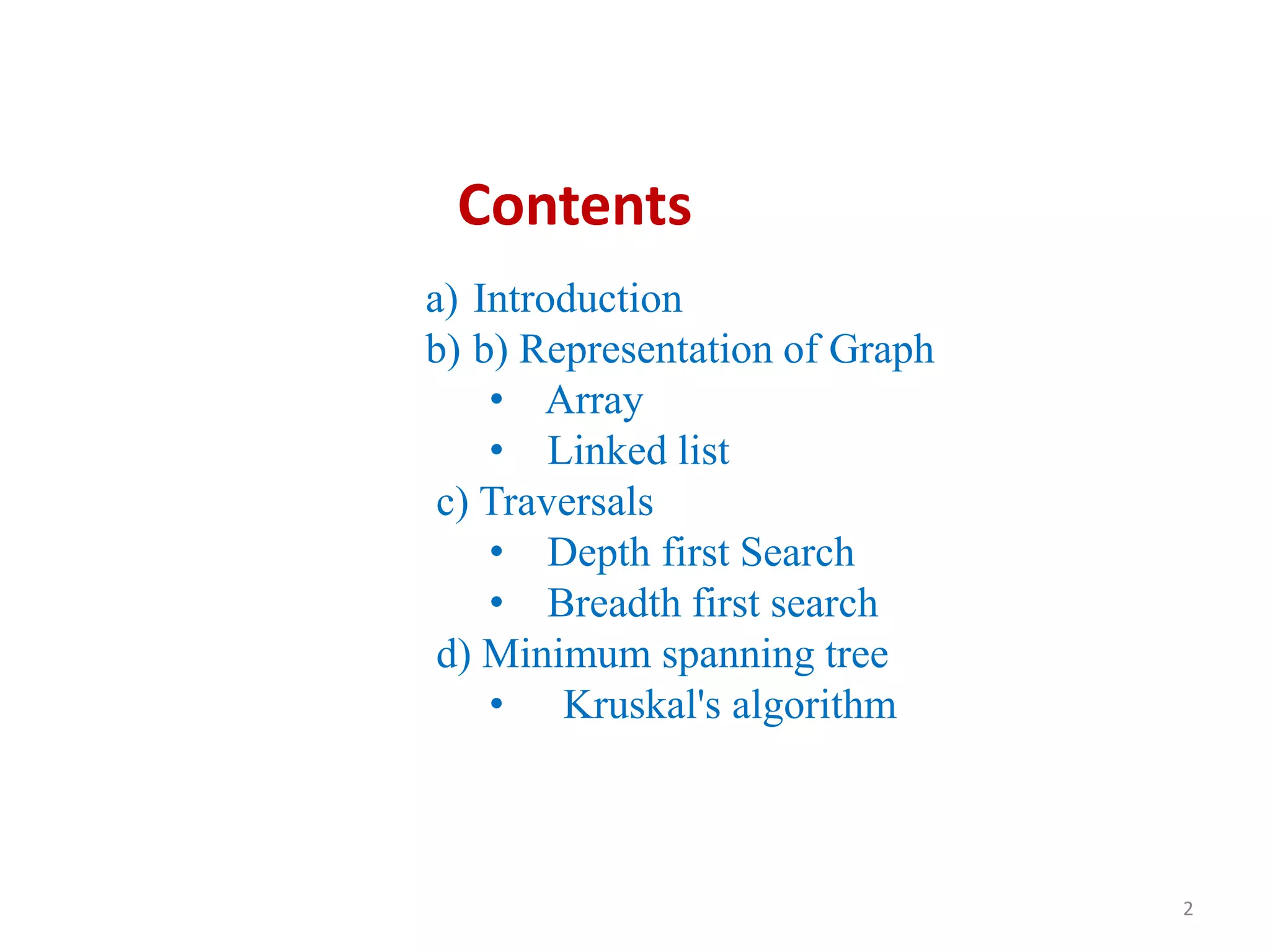
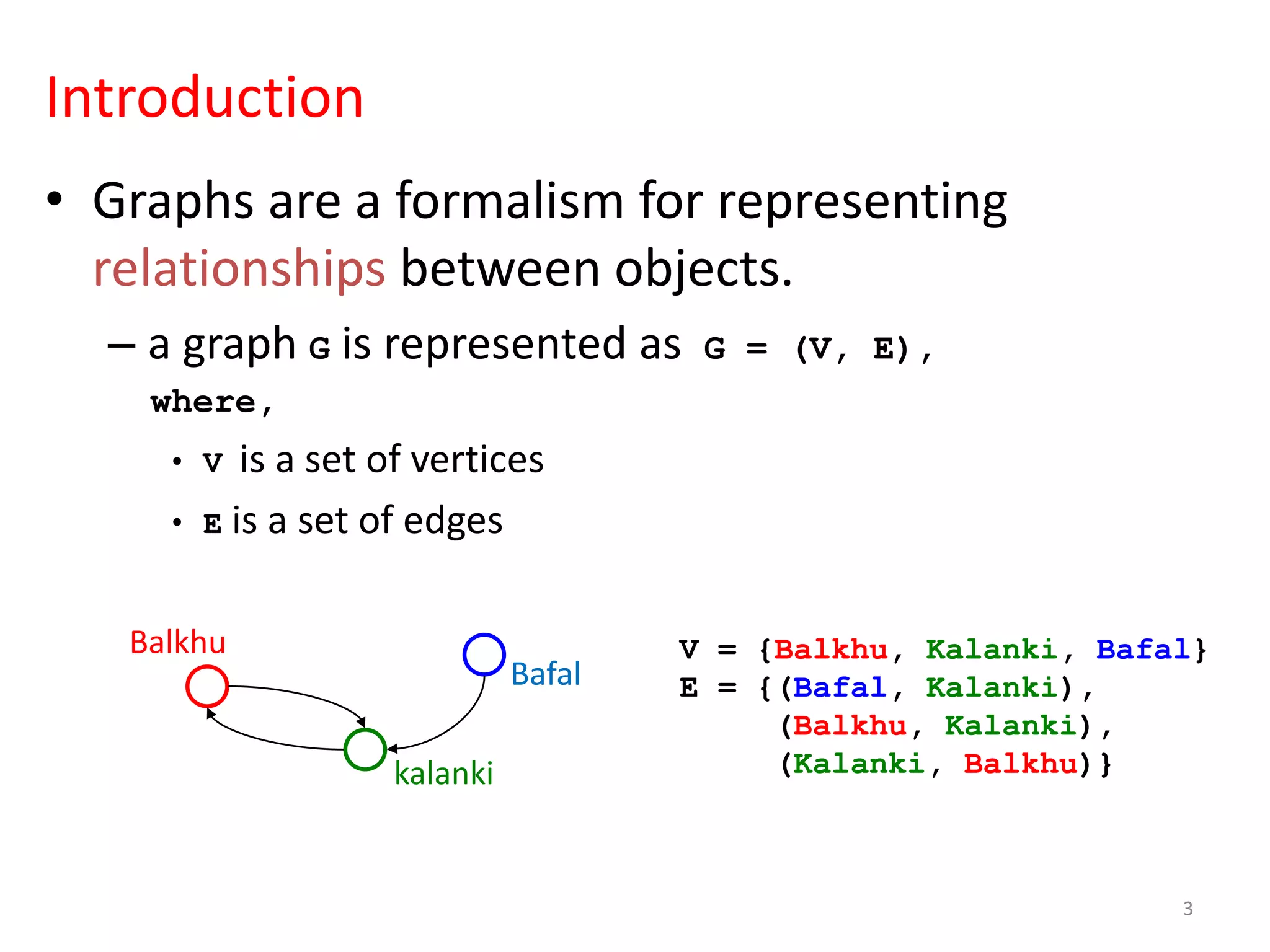
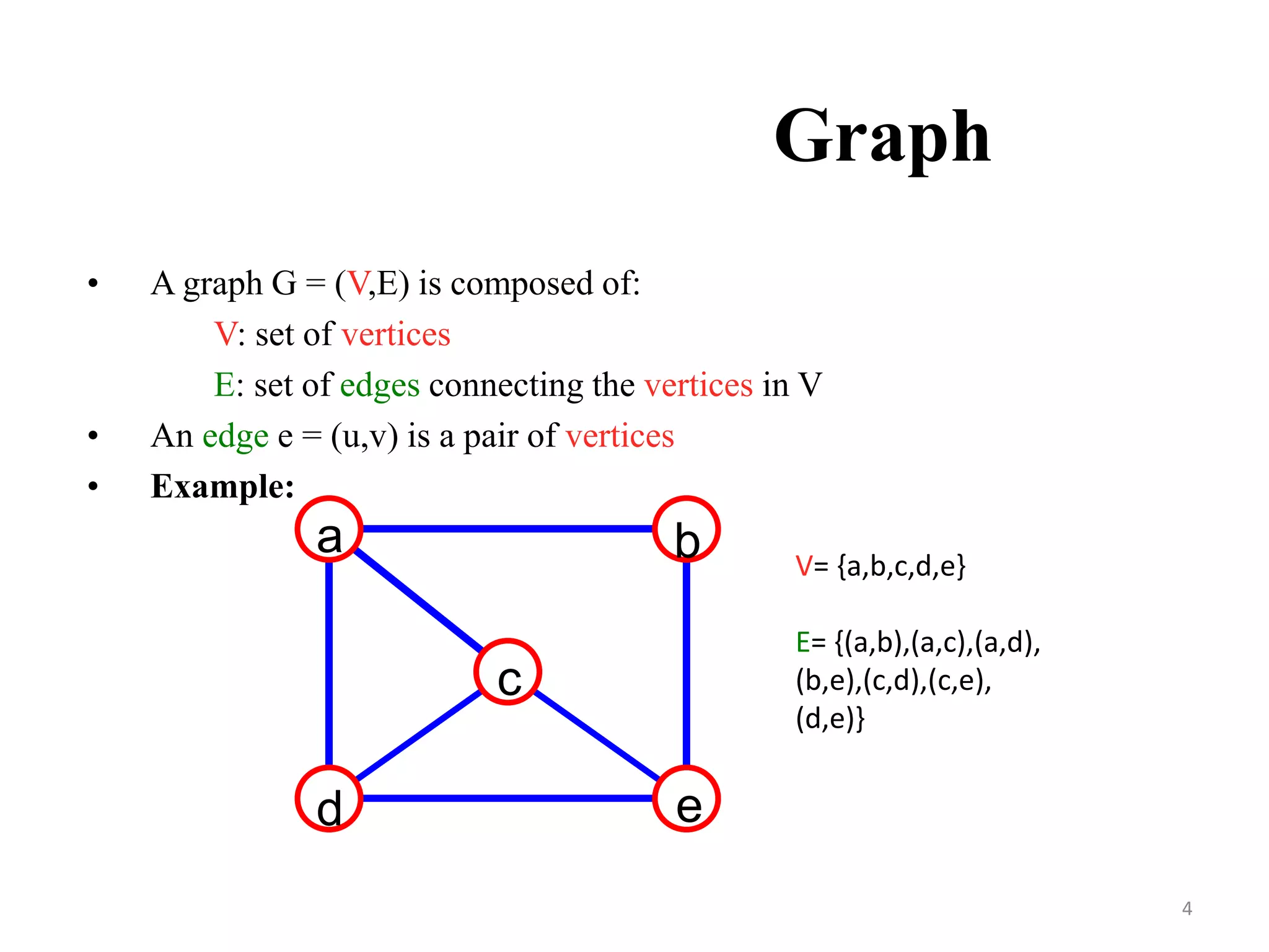
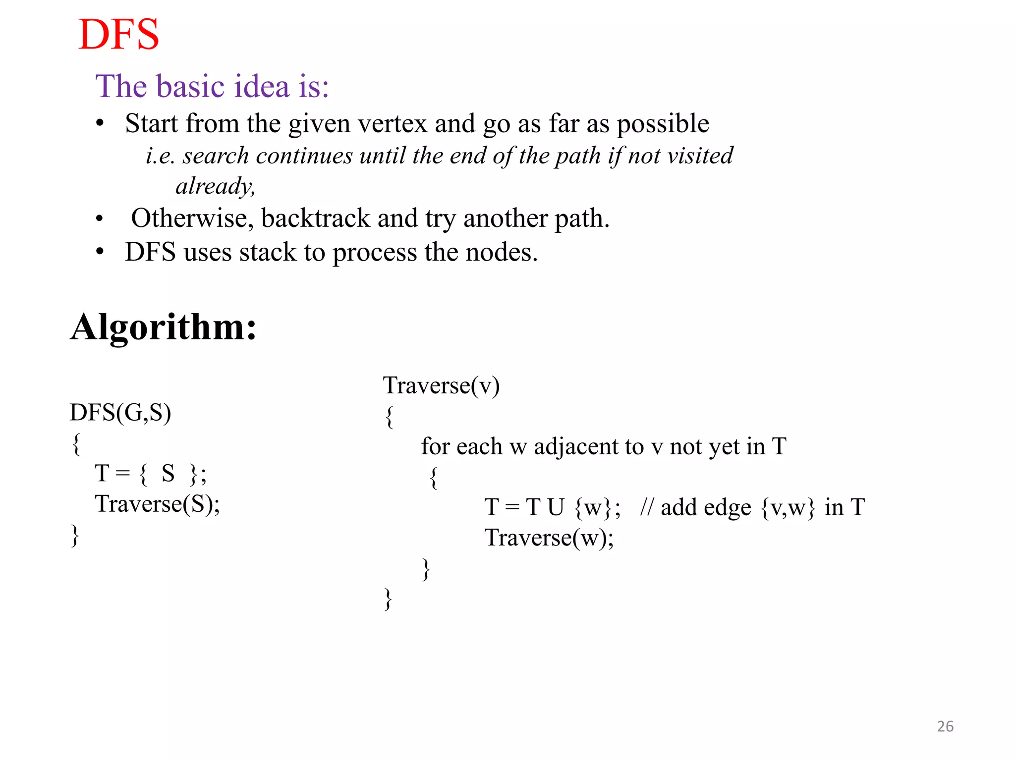
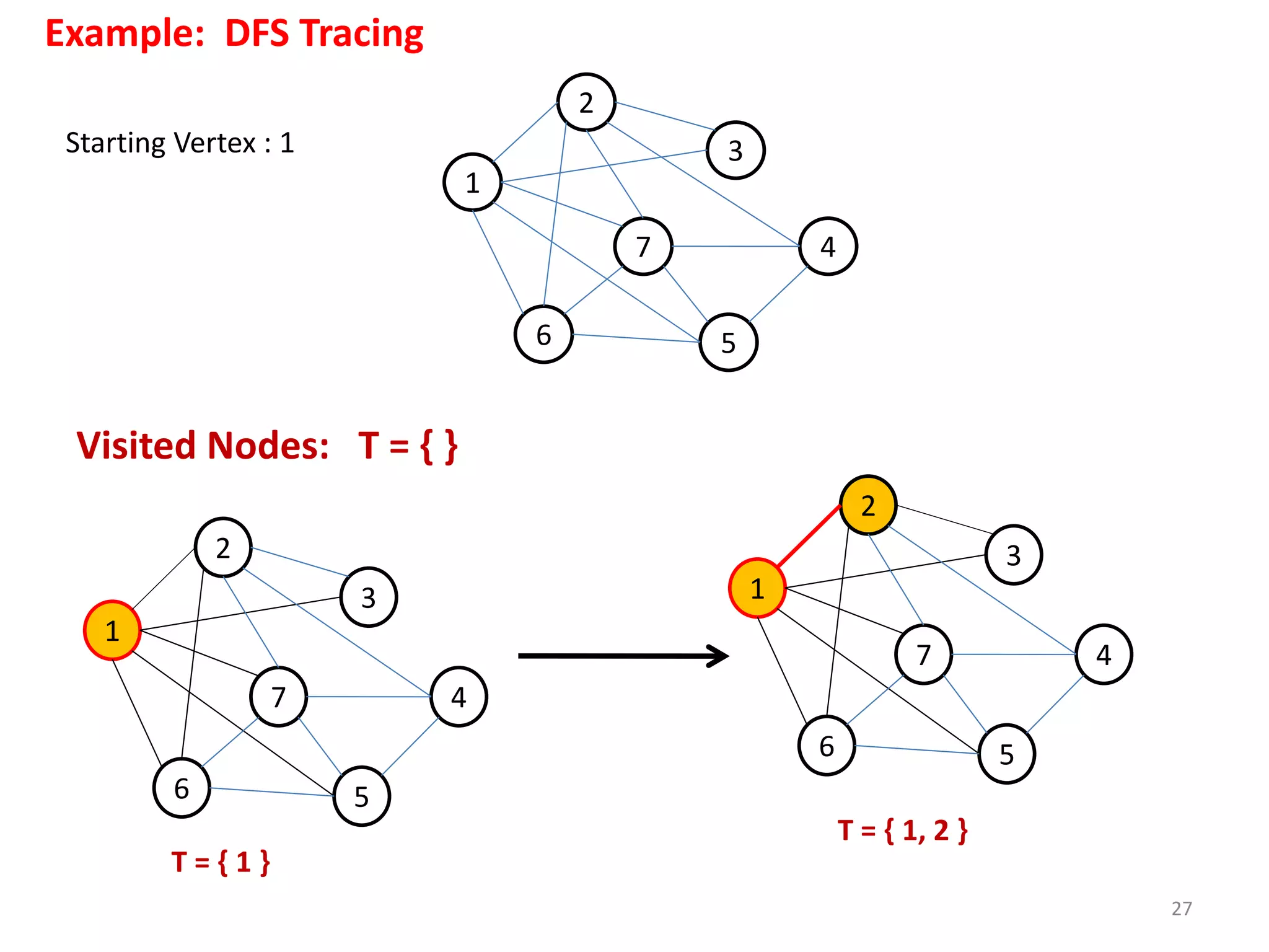
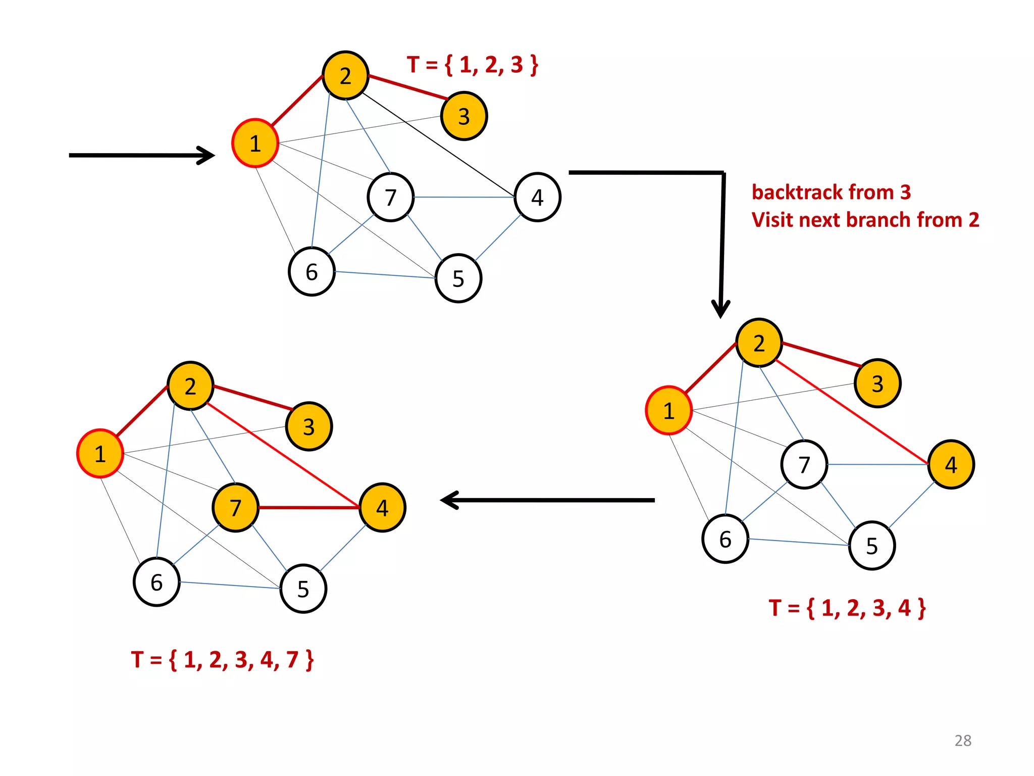
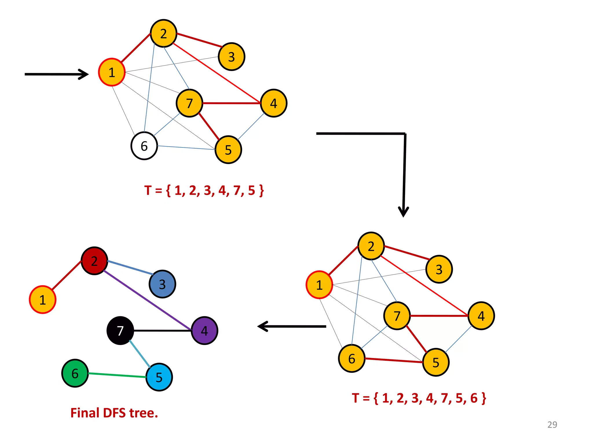
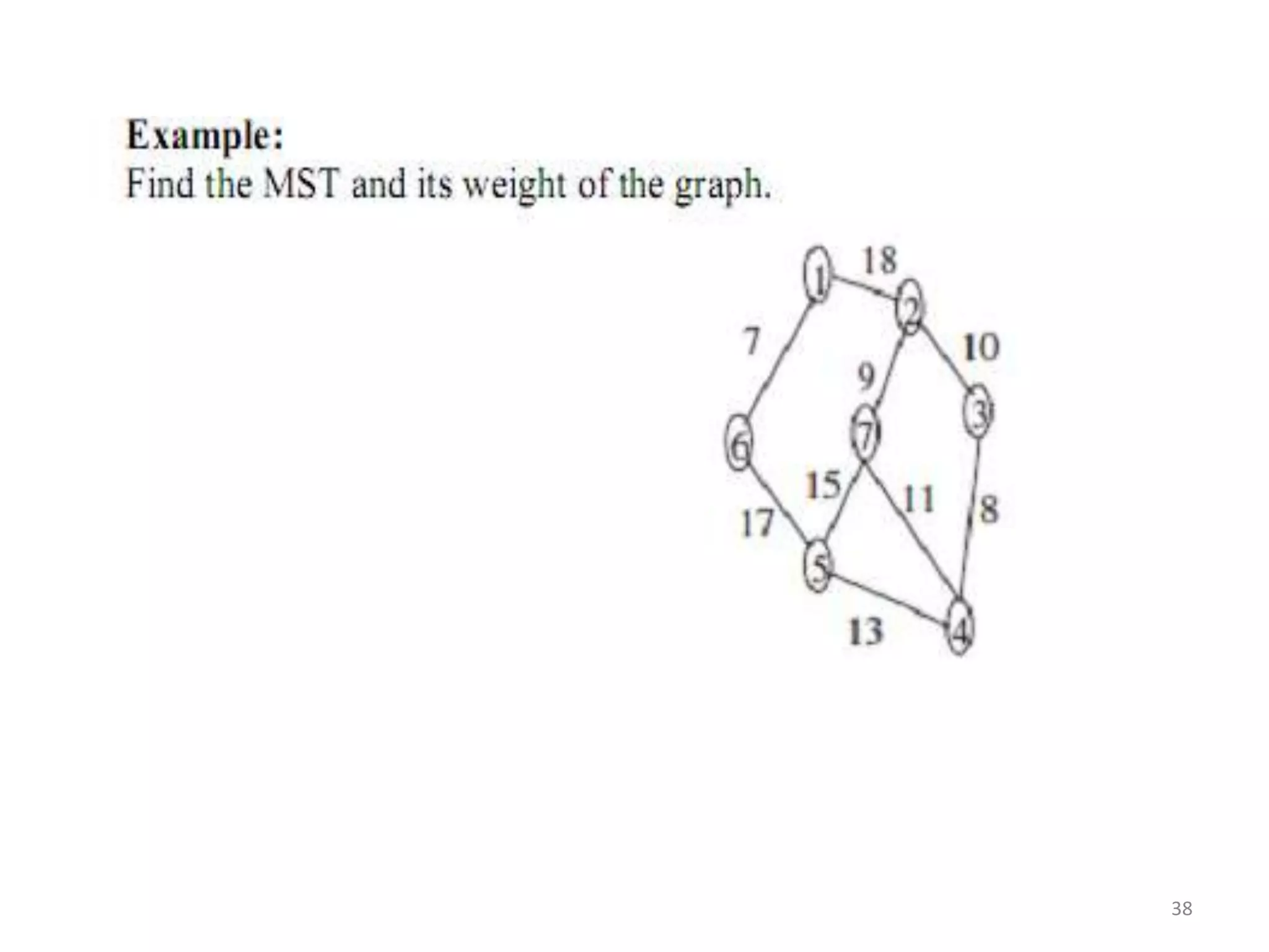
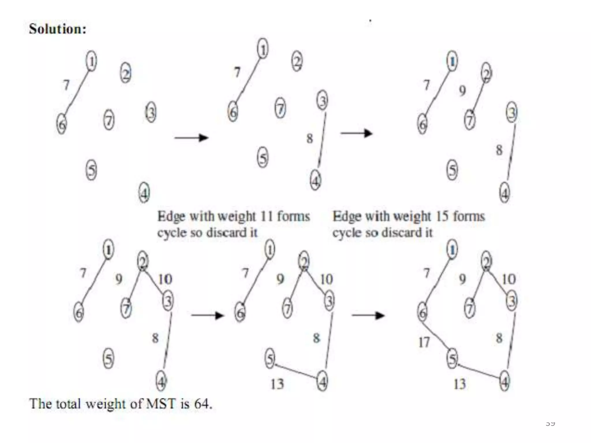
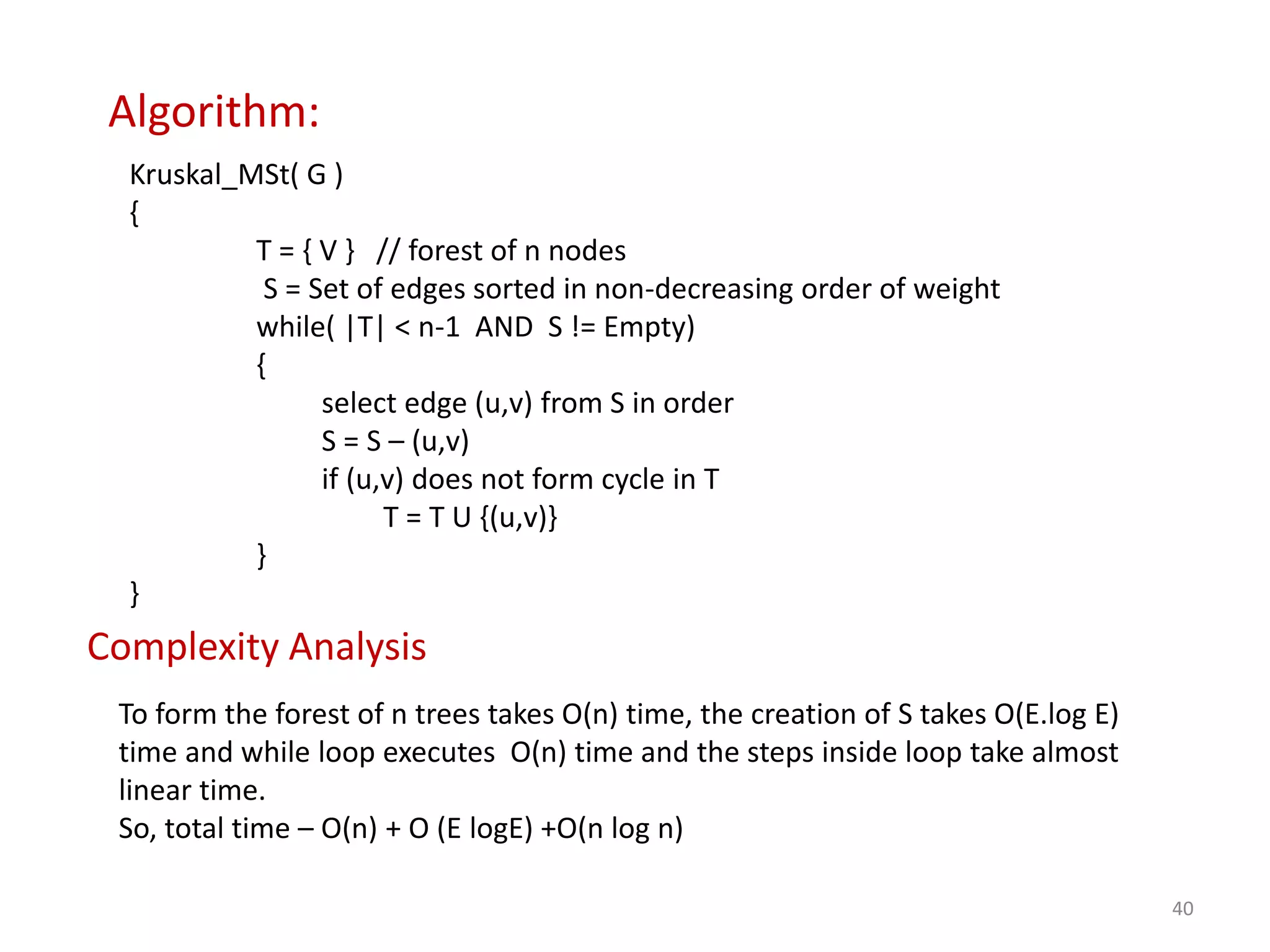
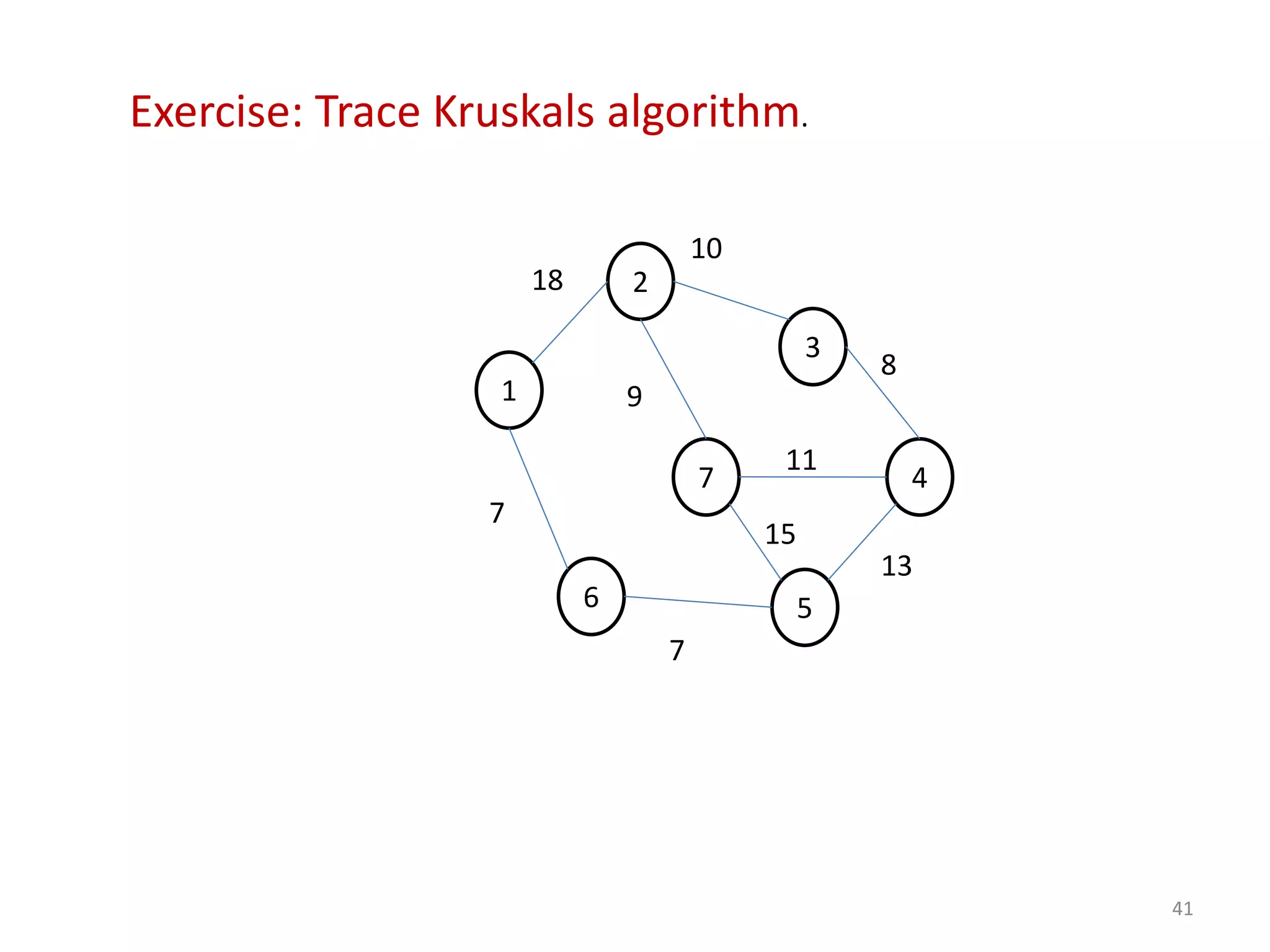
This document provides an overview of graphs and graph algorithms. It begins with an introduction to graphs, including definitions of vertices, edges, directed/undirected graphs, and graph representations using adjacency matrices and lists. It then covers graph traversal algorithms like depth-first search and breadth-first search. Minimum spanning trees and algorithms for finding them like Kruskal's algorithm are also discussed. The document provides examples and pseudocode for the algorithms. It analyzes the time complexity of the graph algorithms. Overall, the document provides a comprehensive introduction to fundamental graph concepts and algorithms.