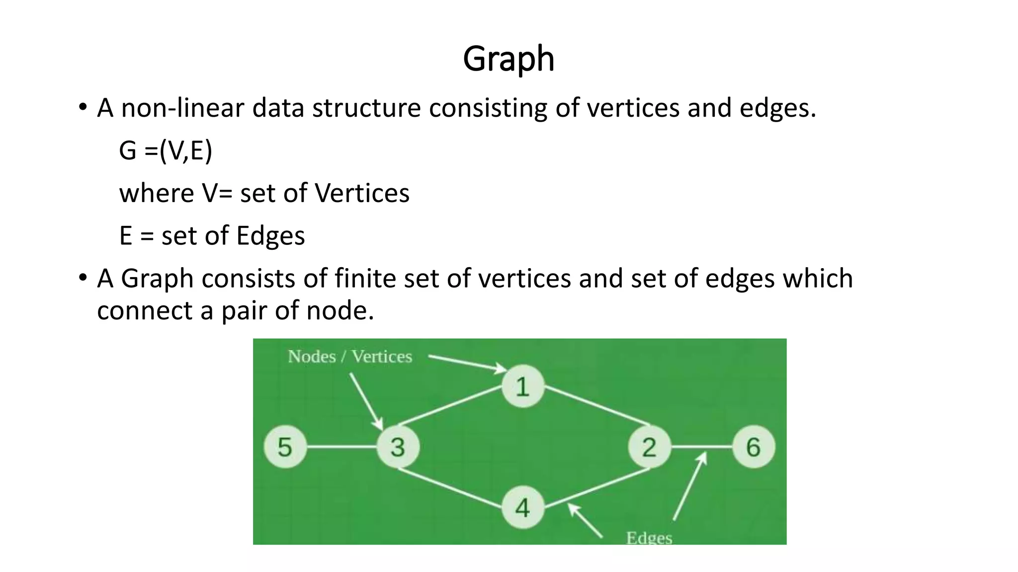
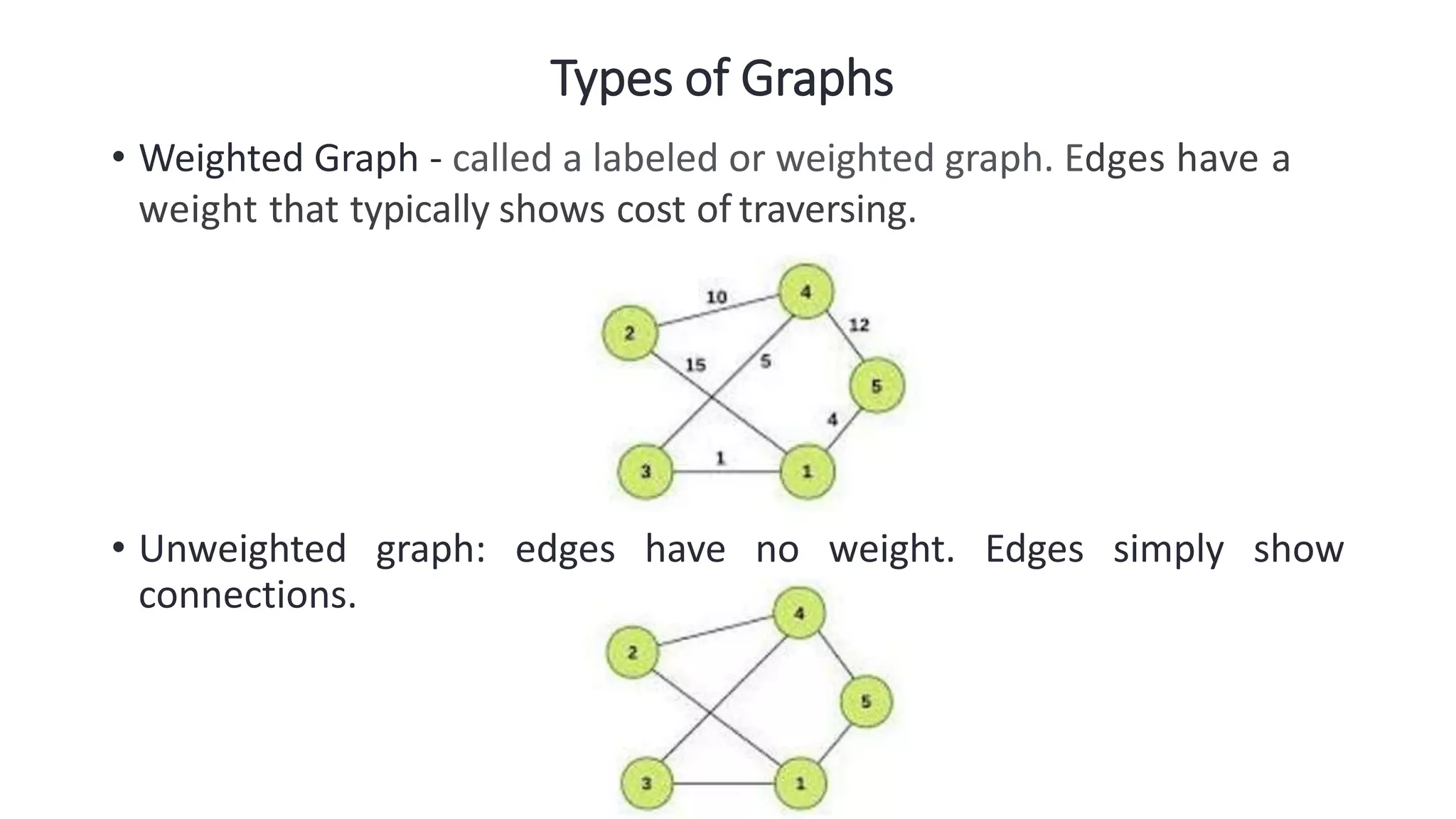
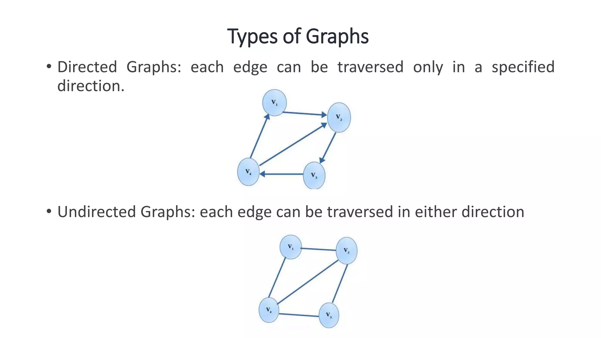
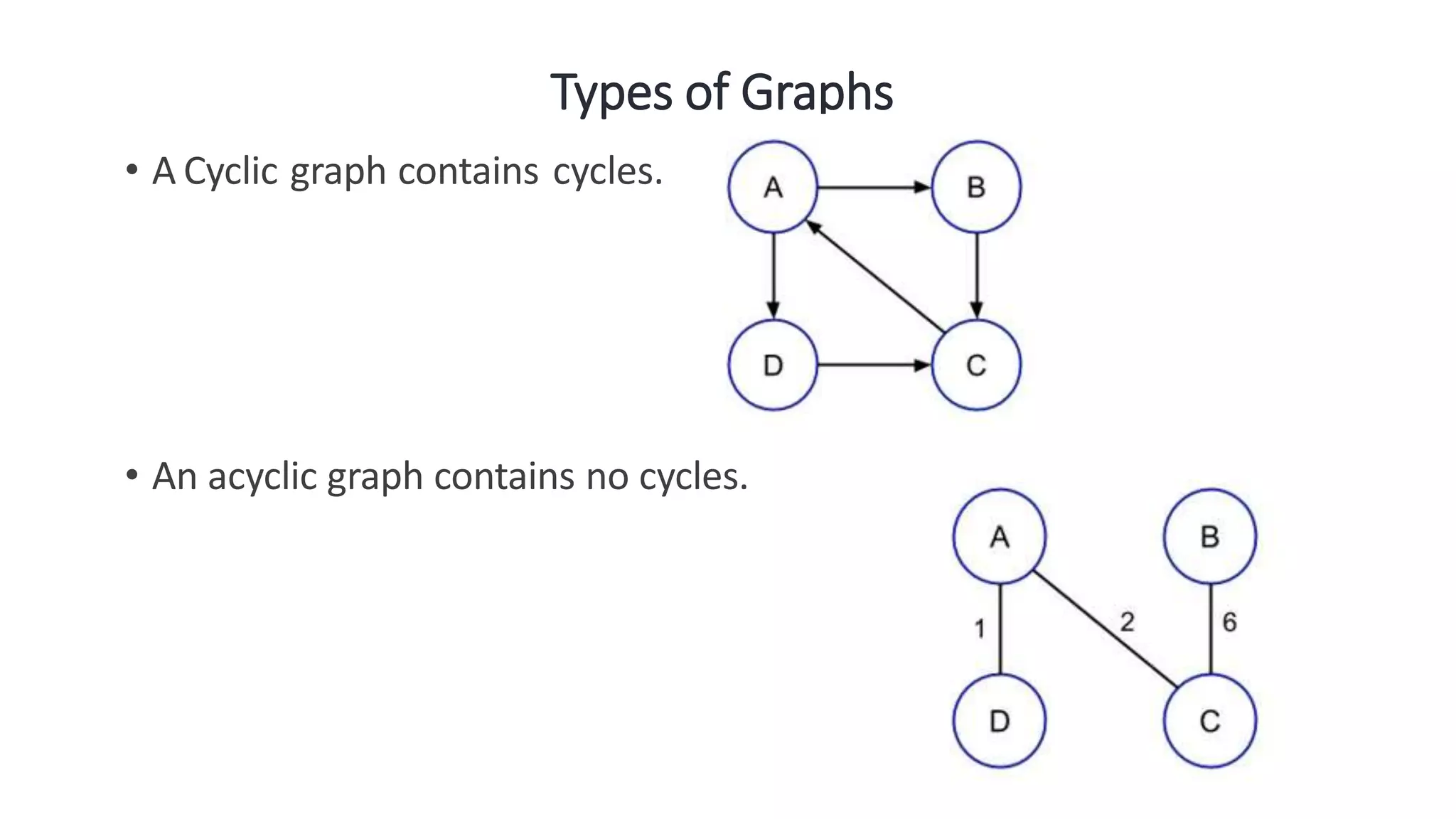
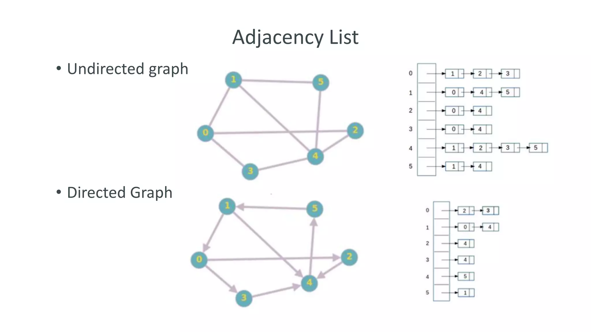
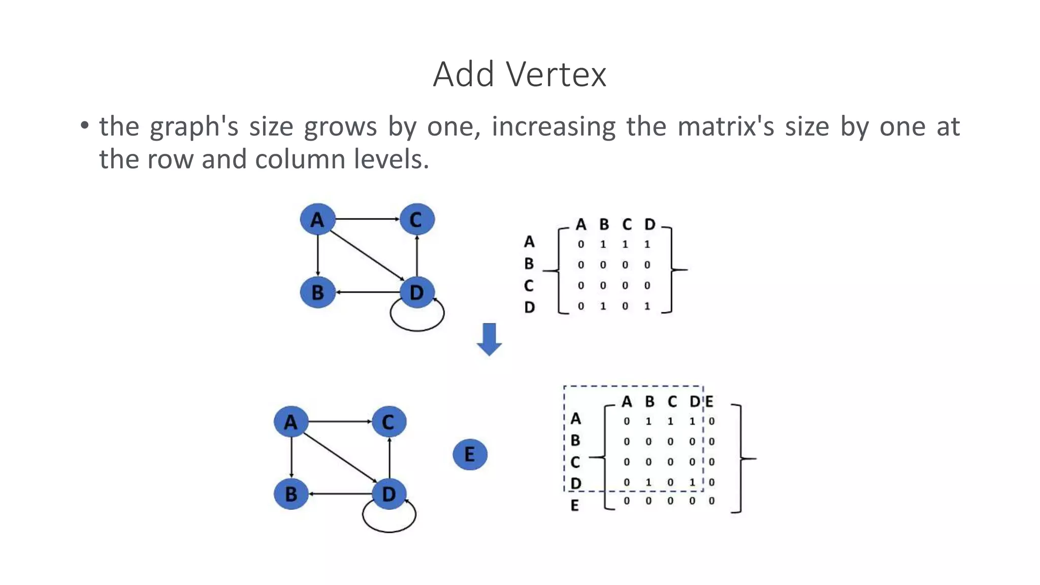
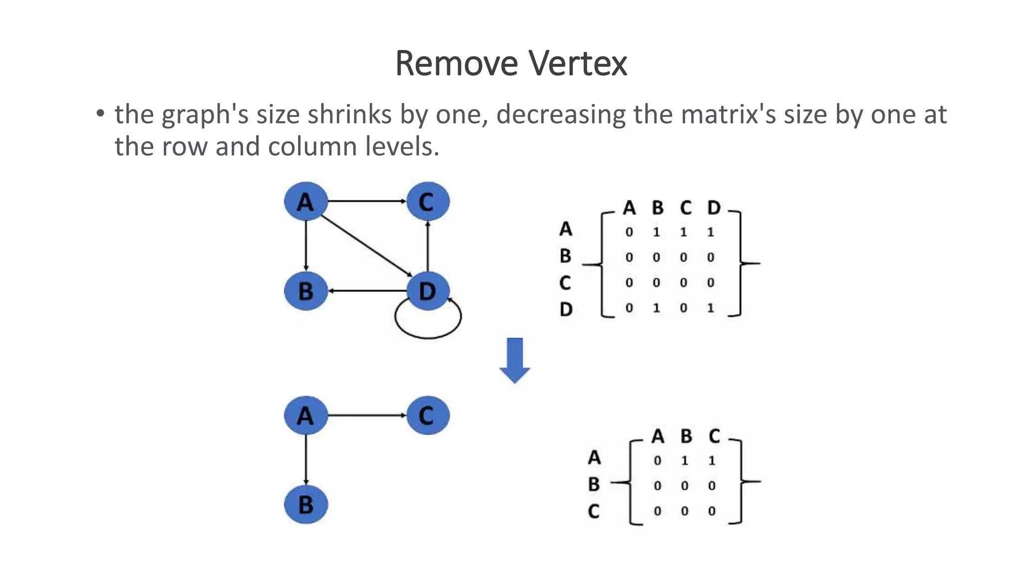
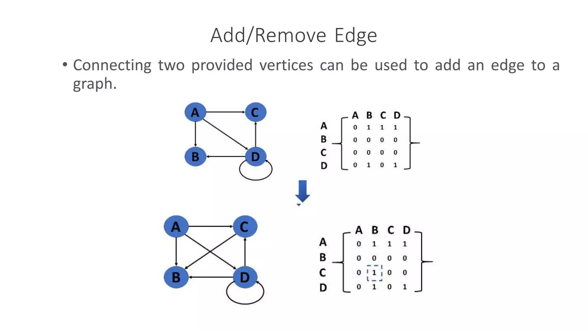
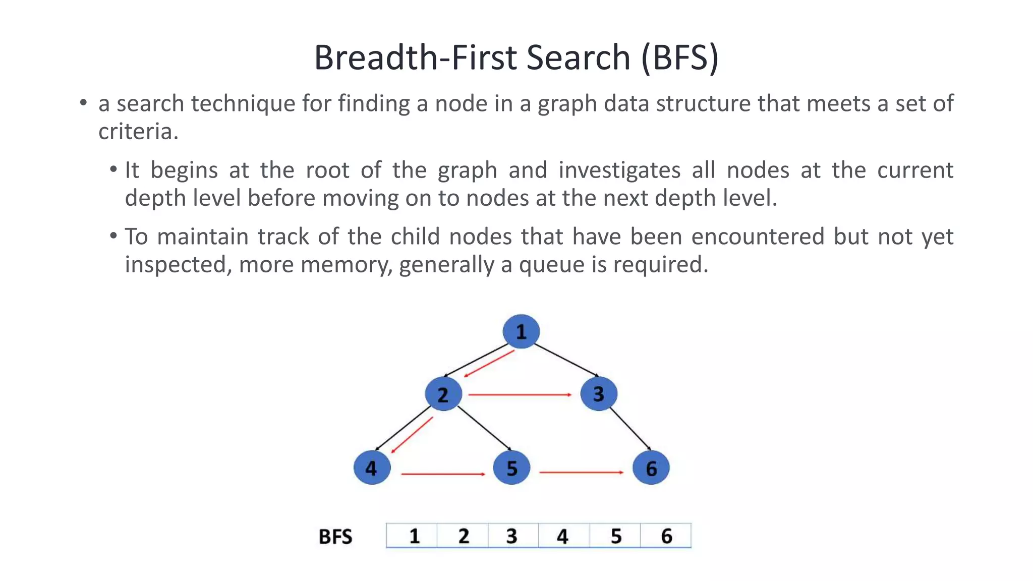
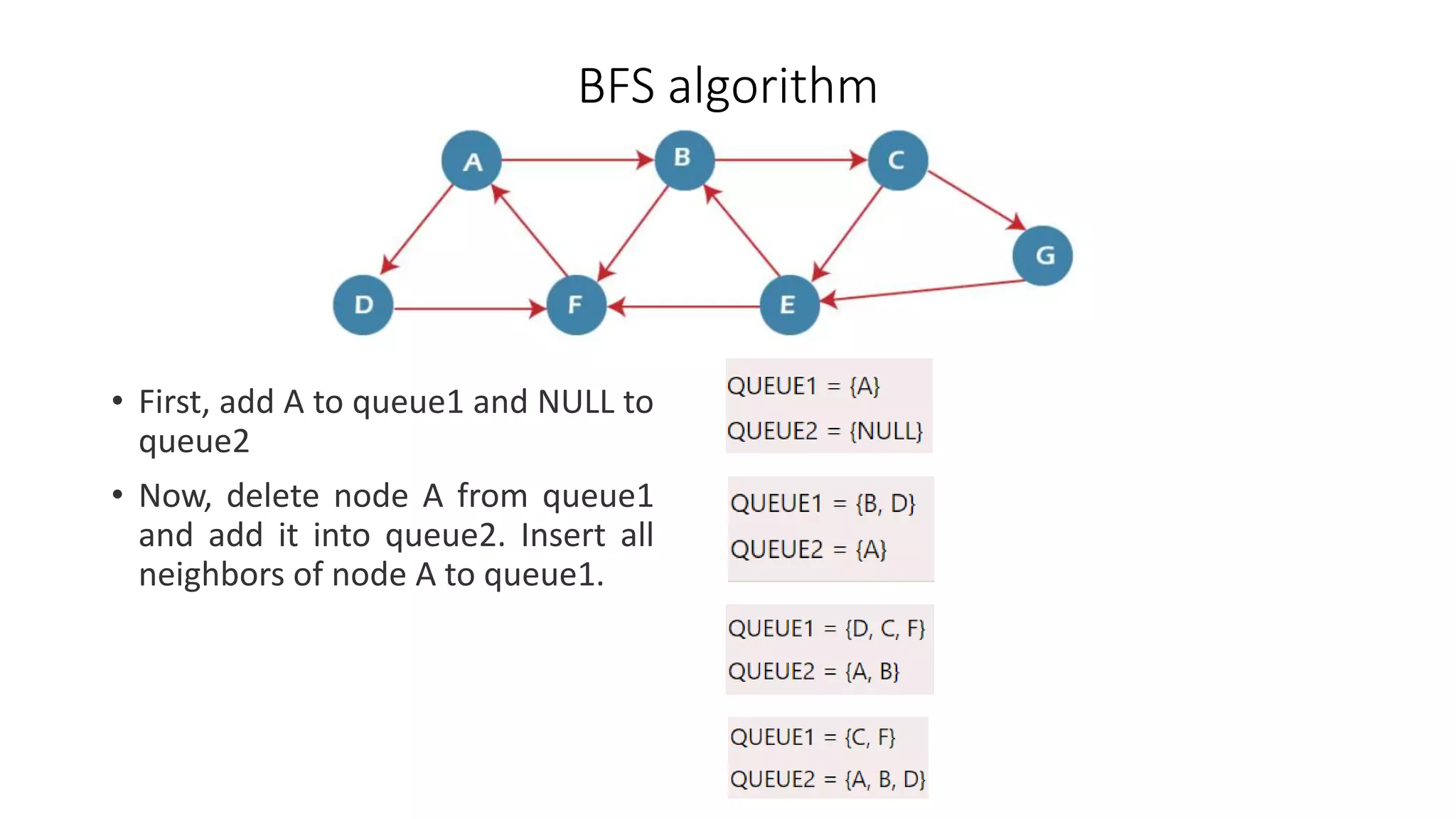
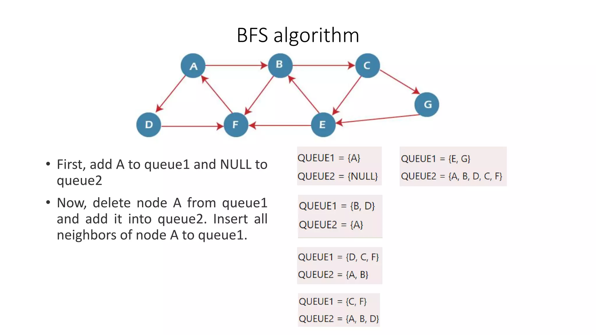
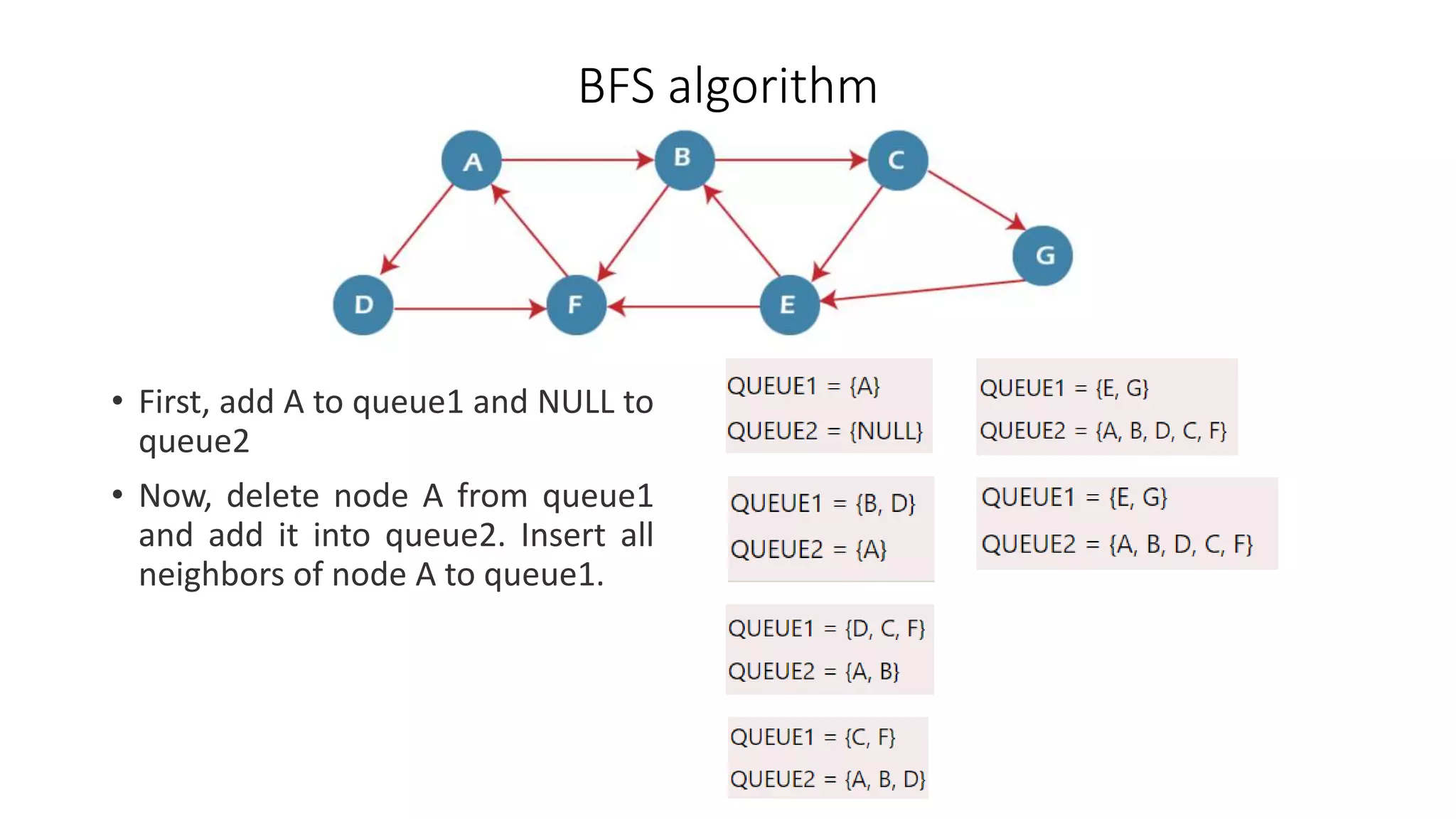
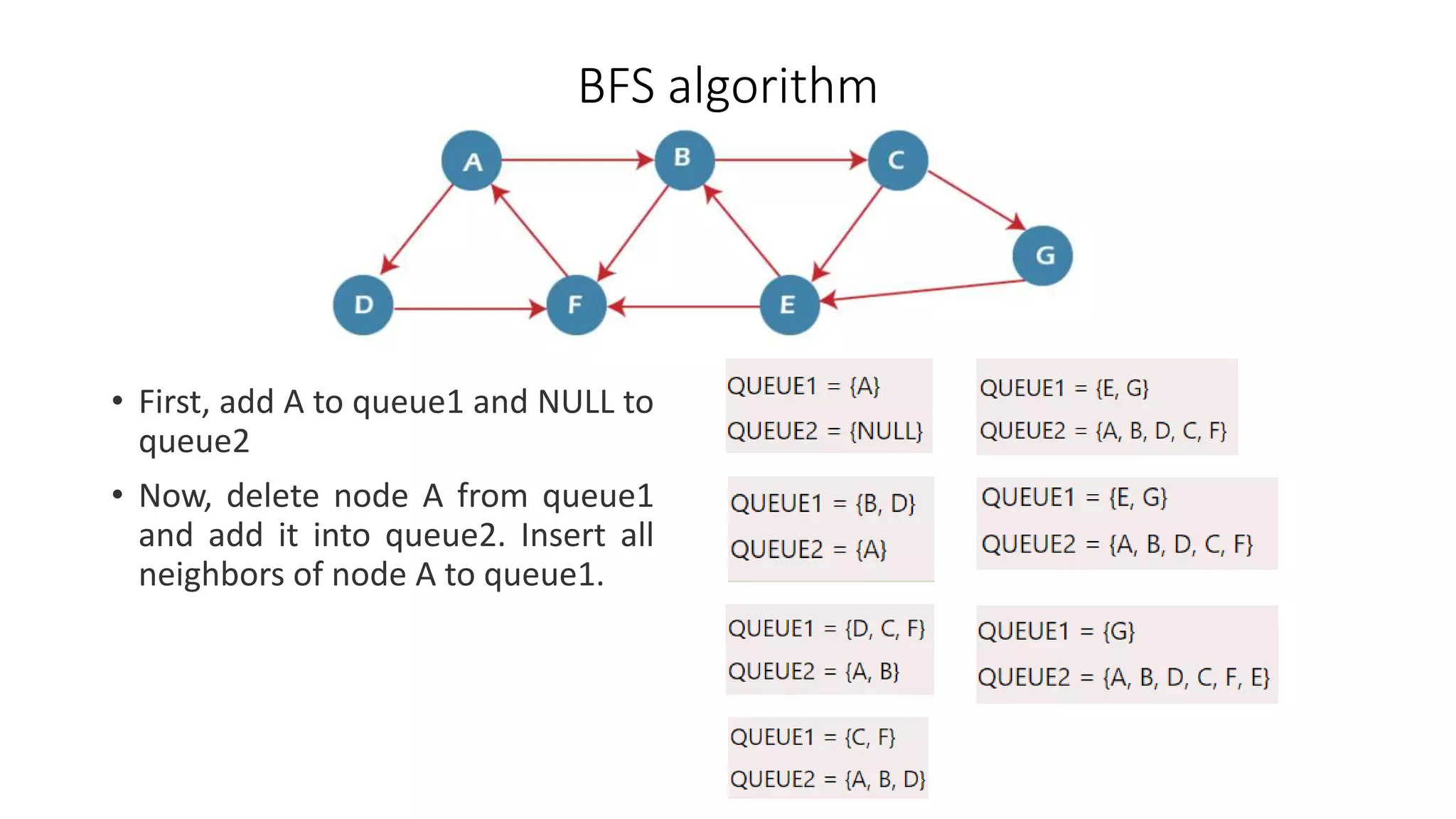
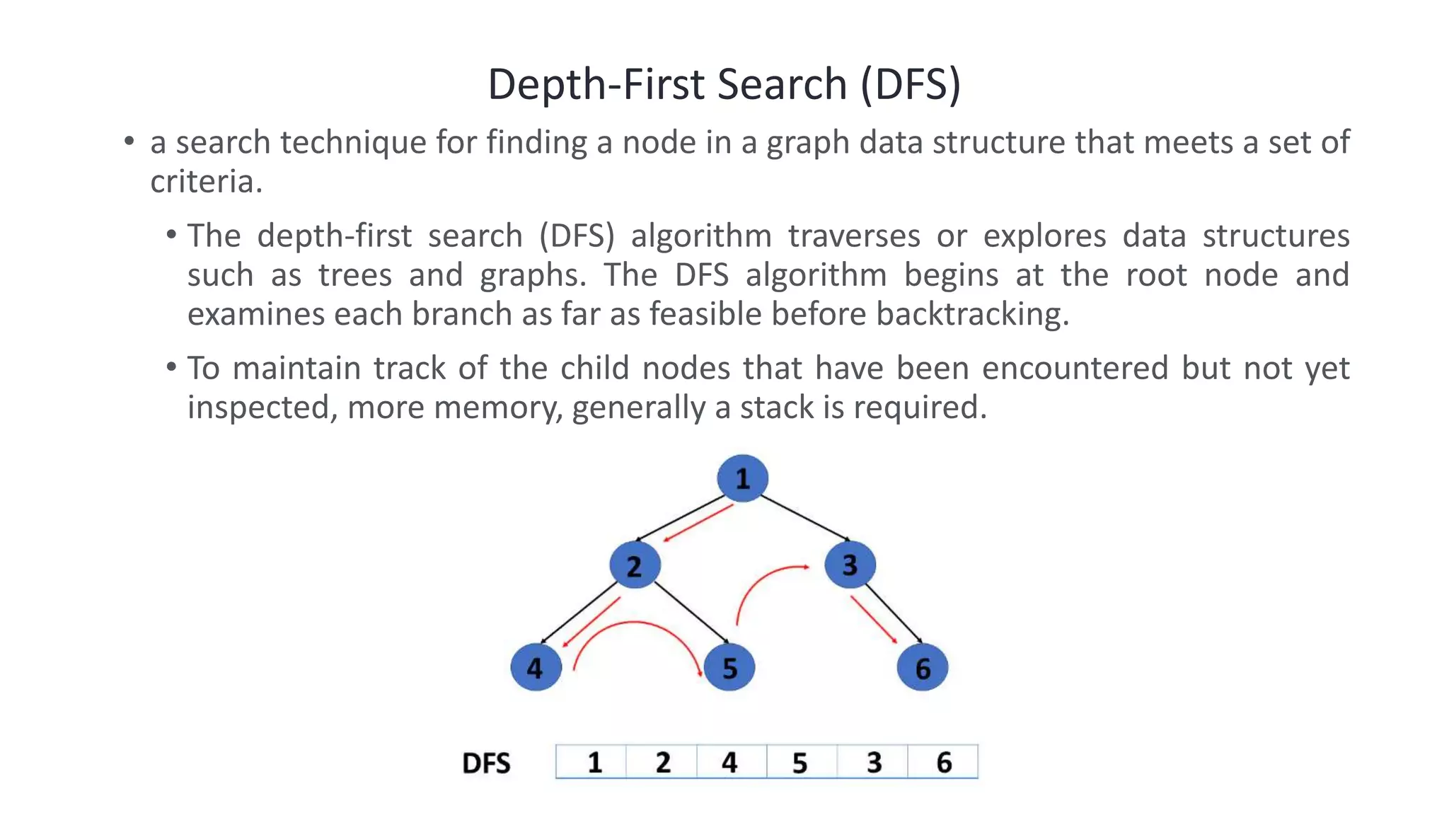
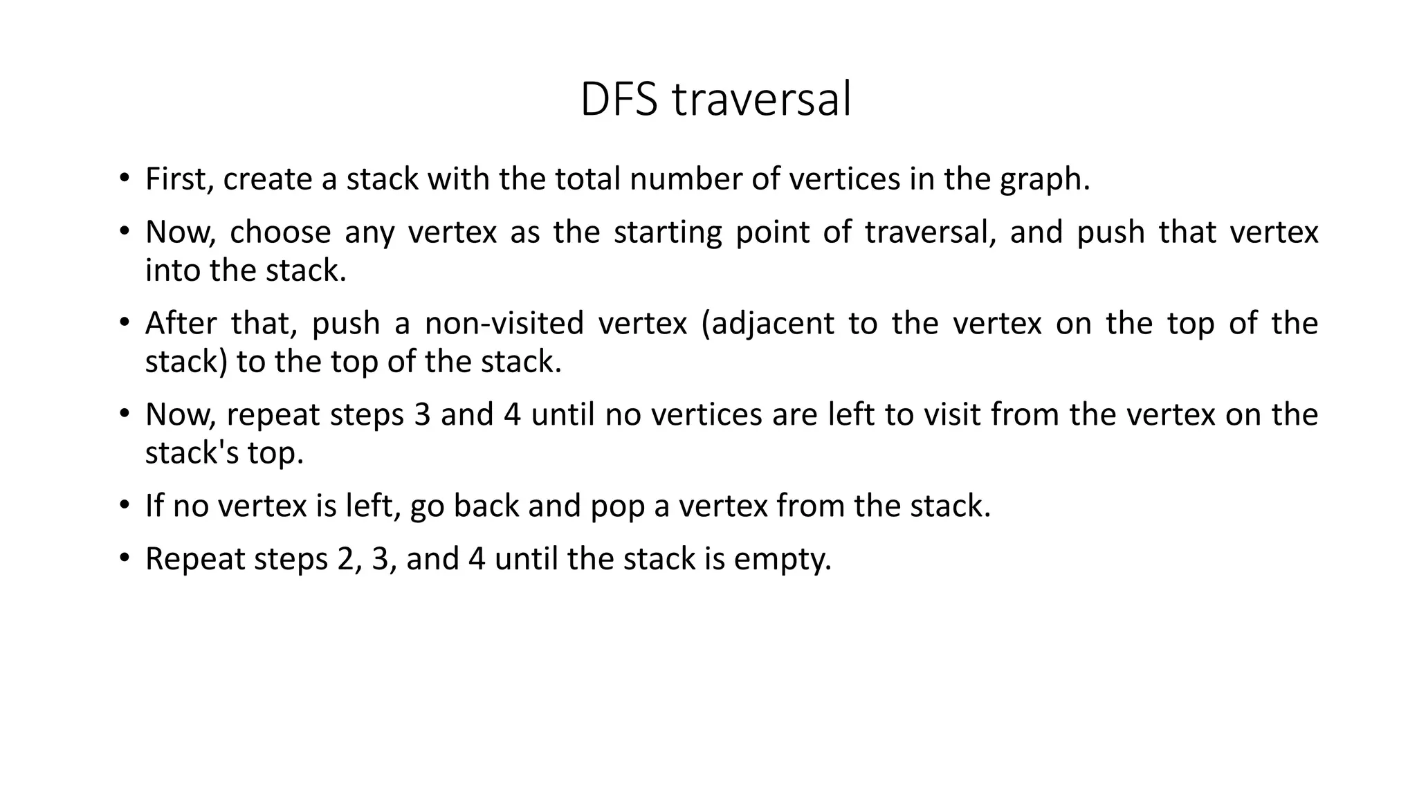
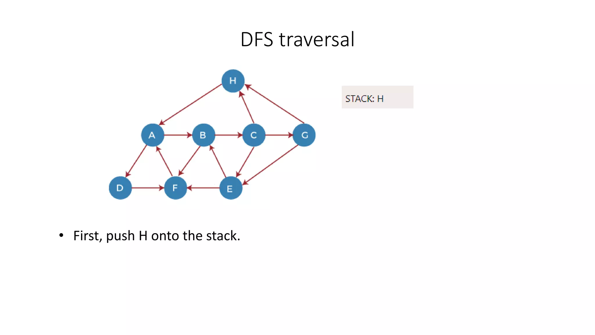
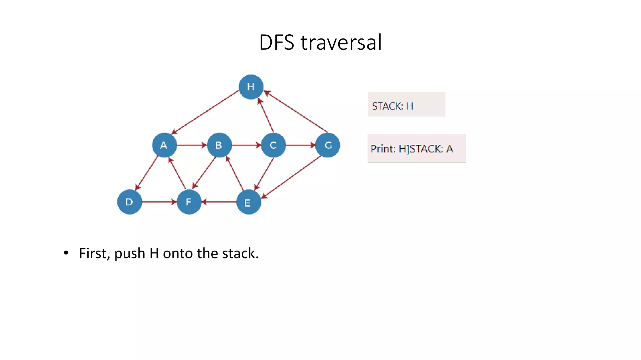
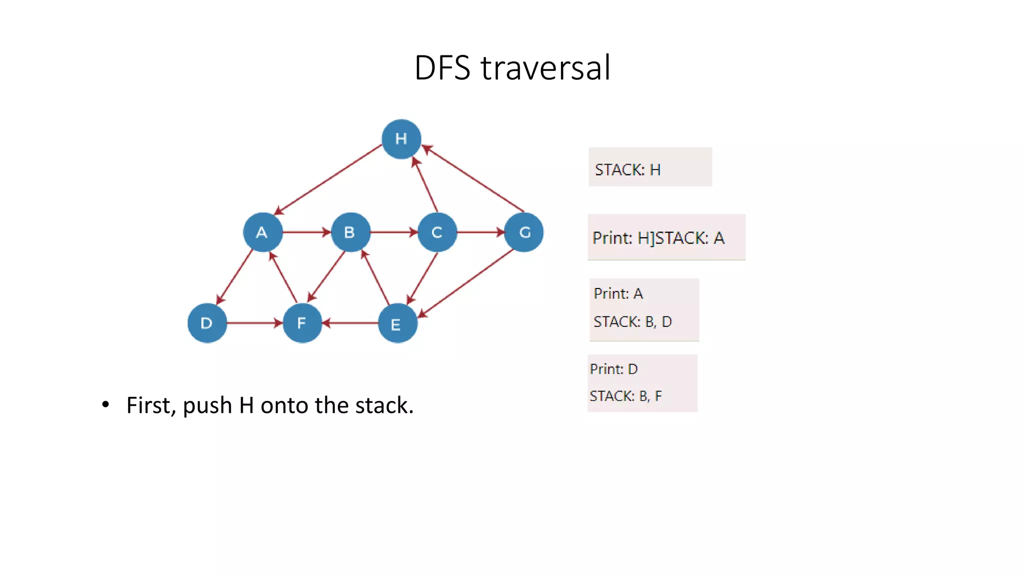
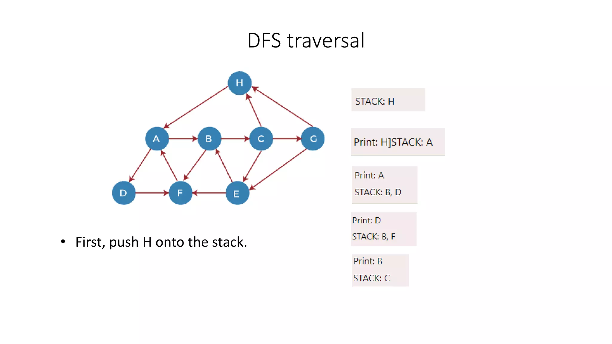
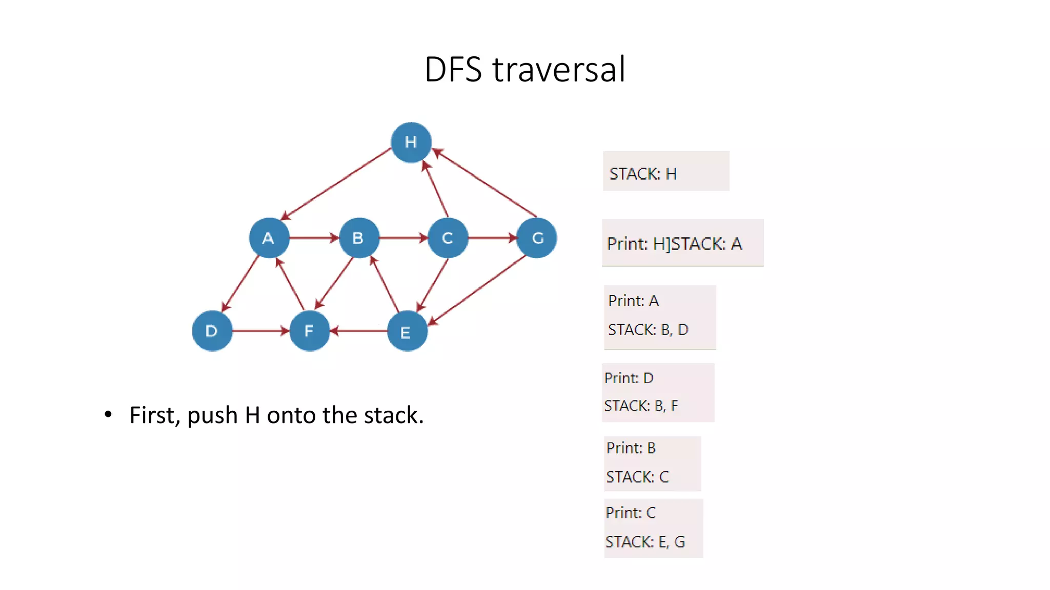
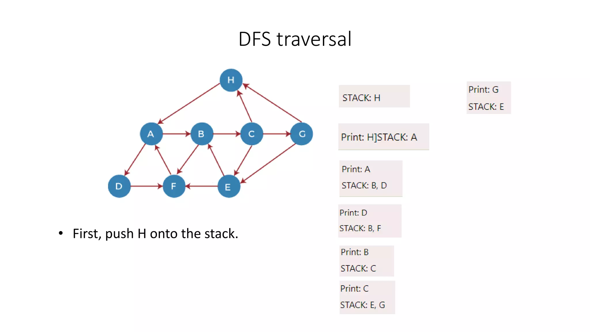
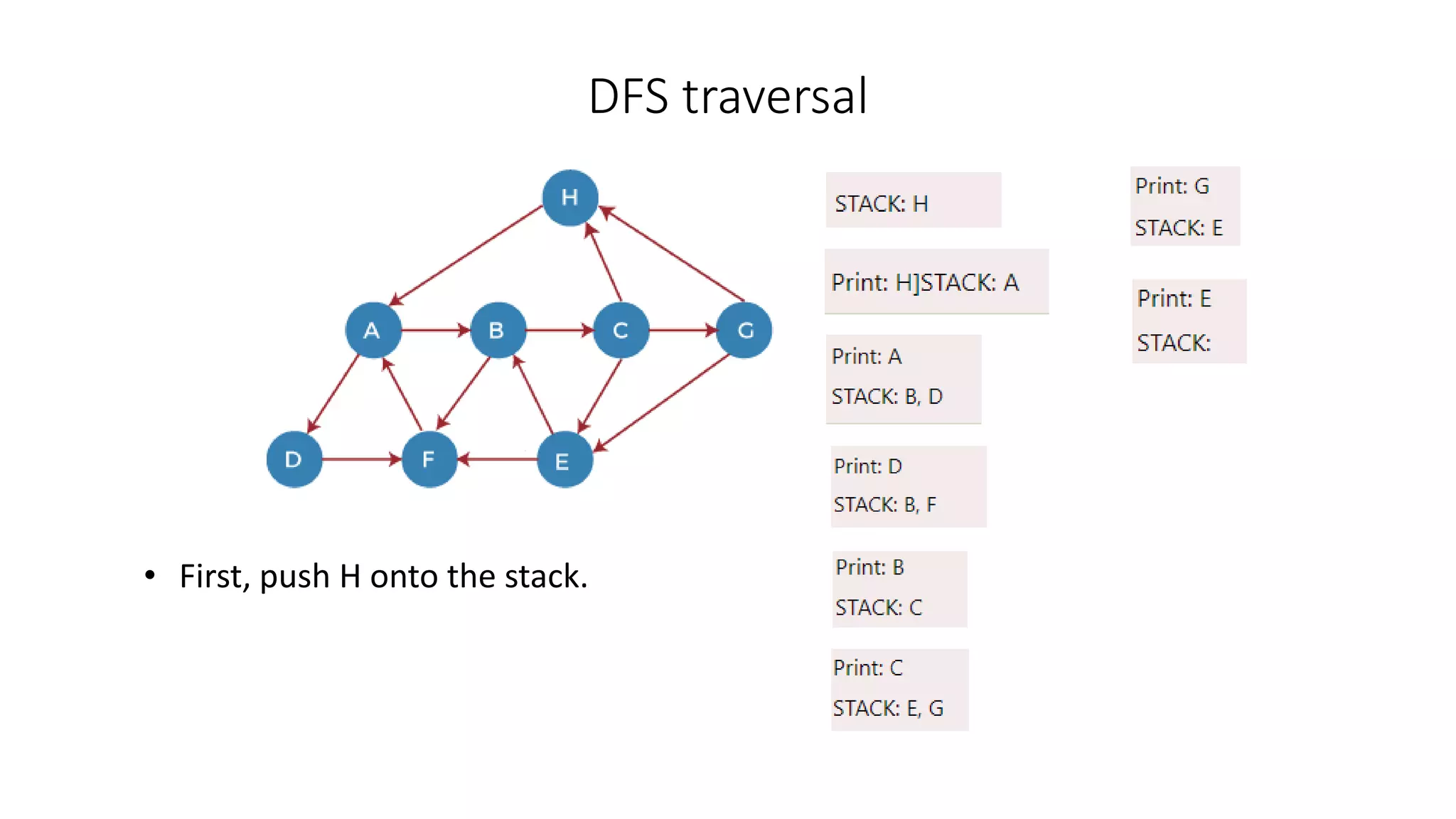
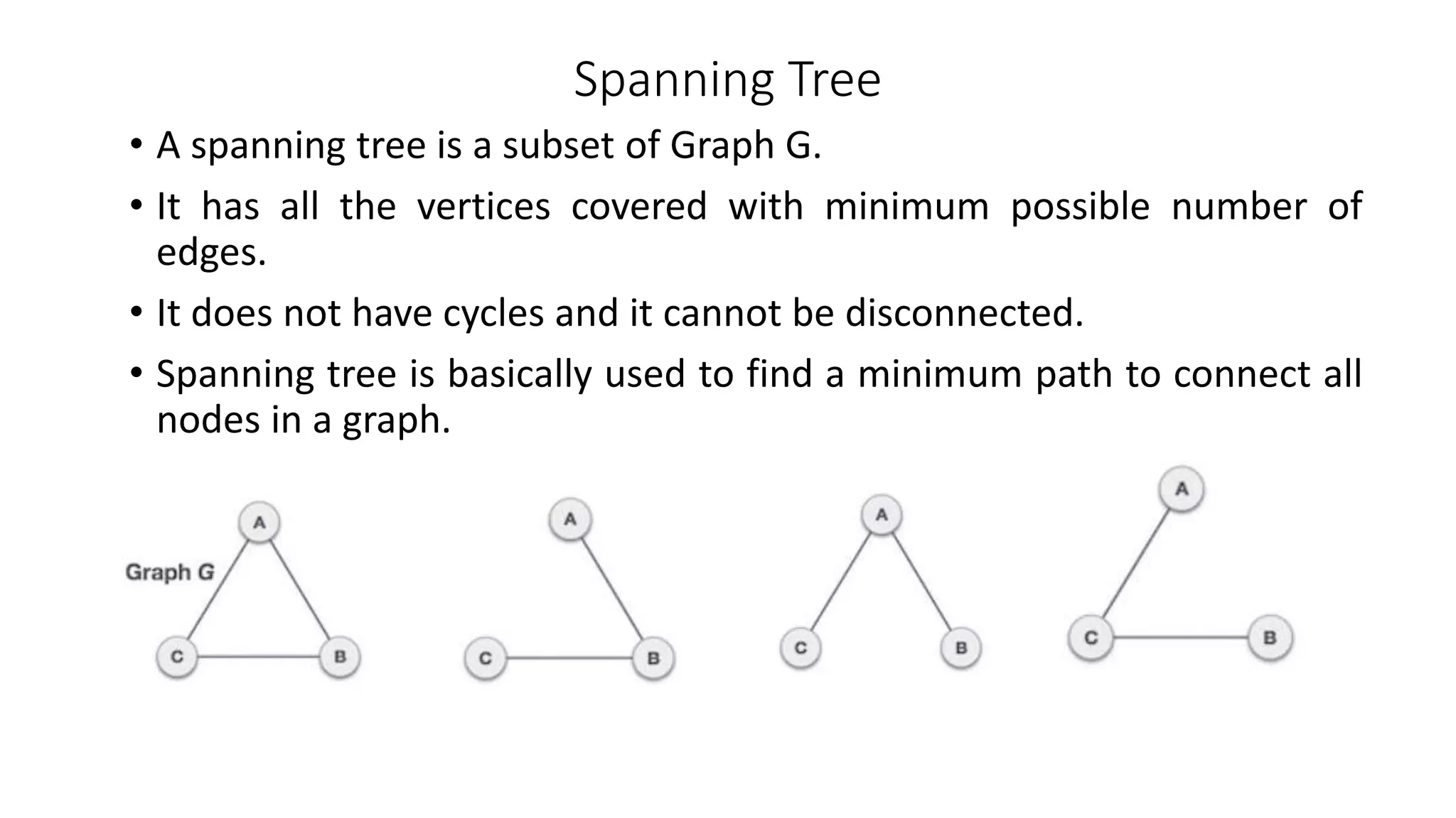
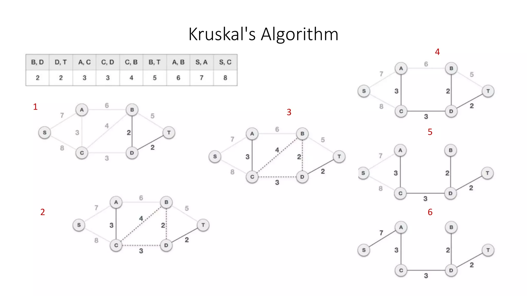
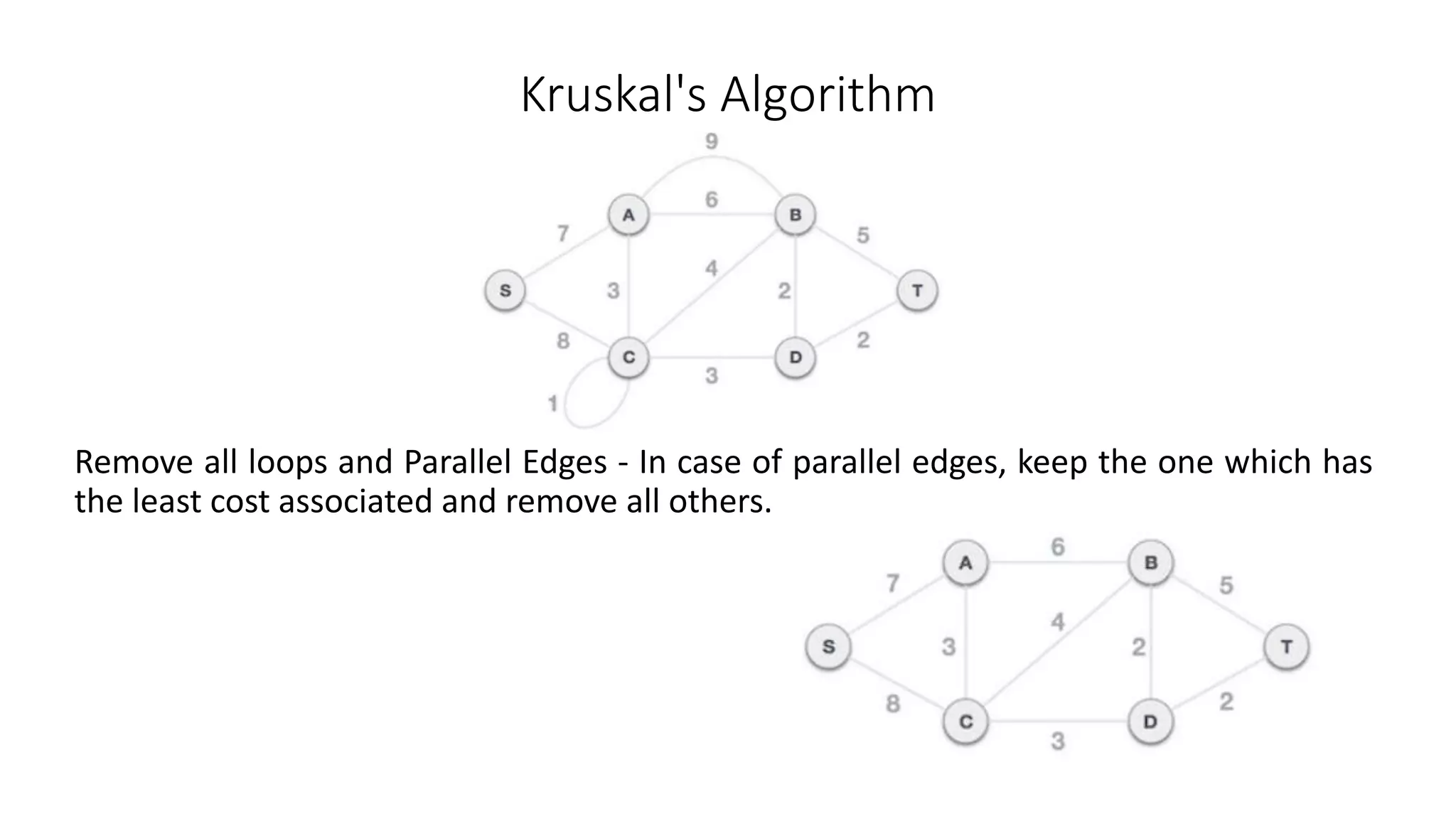
Unit VI
Graphs
Graph
• A non-linear data structure consisting of vertices and edges.
G =(V,E)
where V= set of Vertices
E = set of Edges
• A Graph consists of finite set of vertices and set of edges which
connect a pair of node.
Terminologies
• Vertex − Each node of the graph is represented as a vertex.
• Edge − Edge represents a path between two vertices or a line
between two vertices.
• Adjacency − Two node or vertices are adjacent if they are connected
to each other through an edge.
• Path − Path represents a sequence of edges between the two
vertices.
• Degree of a node – is the number of edges the node is used to define
• In – degree – Number of edges pointing to a node
• Out – degree – Number of edges pointing from a node
Terminologies
• Cycle – a path that starts and ends on the same vertex.
• Simple path – a path that does not cross itself.
• Length of a path: Number of edges in the path.
• An undirected graph is connected if every pair of vertices has a path
between it.
• A directed graph is strongly connected if every pair of vertices has a
path between them, in both directions
Types of Graphs
• Weighted Graph - called a labeled or weighted graph. Edges have a
weight that typically shows cost of traversing.
• Unweighted graph: edges have no weight. Edges simply show
connections.
Types of Graphs
• Directed Graphs: each edge can be traversed only in a specified
direction.
• Undirected Graphs: each edge can be traversed in either direction
Types of Graphs
• A Cyclic graph contains cycles.
• An acyclic graph contains no cycles.
Applications ofgraphs
• To represent networks. The networks may include paths in a city or
telephone network or circuit network.
• In social networks like linkedIn, Facebook. For example, in Facebook,
each person is represented with a vertex(or node). Each node is a
structure and contains information like person id, name, gender, etc.
Applications ofgraphs
• Electrical Engineering − extensively used in designing circuit connections.
• Computer Network − The relationships among interconnected computers
in the network follows the principles of graph theory.
• Science − The molecular structure and chemical structure of a substance,
the DNA structure of an organism, etc., are represented by graphs.
• Linguistics − The parsing tree of a language and grammar of a language
uses graphs.
Graphs
• Graphs can also be defined in the form of matrices.
• To perform the calculation of paths and cycles in the graphs, matrix
representation is used.
• It is calculated using matrix operations.
• The two most common representation of the graphs are:
• Adjacency Matrix
• Adjacency List
AdjacencyMatrix
• is nothing but a square matrix utilised to describe a finite graph.
• also called the connection matrix.
• is a matrix containing rows and columns which is used to represent a
simple labelled graph, with 0 or 1.
• If a graph has n number of vertices, then the adjacency matrix
of that graph is n x n, and each entry of the matrix represents
the number of edges from one vertex to another.
• Sometimes it is also called a Vertex matrix.
Adjacency matrix for an undirected graph
• edges are not associated with the directions with them.
Adjacency matrix for a directed graph
Adjacency matrix for the undirected weighted graph
Adjacency matrix for the directed weighted graph
Adjacency List
• a list that helps you keep track each node’s neighbor in a graph.
• is an array of separate lists.
• Each element of array is a list of corresponding neighbour (or directly
connected) vertices.
• This representation is based on Linked Lists.
• At the end of list, each node is connected with the null values to tell
that it is the end node of that list.
Adjacency List
• Undirected graph
• Directed Graph
Operations onGraphs
• Add/Remove Vertex
• Add/Remove Edge
• Traverse a graph
Add Vertex
• the graph's size grows by one, increasing the matrix's size by one at
the row and column levels.
Remove Vertex
• the graph's size shrinks by one, decreasing the matrix's size by one at
the row and column levels.
Add/Remove Edge
• Connecting two provided vertices can be used to add an edge to a
graph.
Remove Edge
• The connection between the vertices or nodes can be removed to
delete an edge
Traverse a graph
• The process of visiting or updating each vertex in a graph is known as
graph traversal.
• The sequence in which they visit the vertices is used to classify such
traversals. Graph traversal is a subset of tree traversal.
• There are two techniques to implement a graph traversal algorithm:
• Breadth-first search
• Depth-first search
Breadth-First Search (BFS)
• a search technique for finding a node in a graph data structure that meets a set of
criteria.
• It begins at the root of the graph and investigates all nodes at the current
depth level before moving on to nodes at the next depth level.
• To maintain track of the child nodes that have been encountered but not yet
inspected, more memory, generally a queue is required.
Breadth-First Traversal
• a graph is similar to Breadth-First Traversal of a tree.
• graphs may contain cycles, the same node may be visited again.
• To avoid processing a node more than once, the vertices are divided
into two categories:
• Visited
• Not visited
Breadth-First Search Algorithm
• starts at the first starting node in a graph and travels it entirely.
• After traversing the first node successfully, it visits and marks the next
non-traversed vertex in the graph.
• in the graph, every node is known.
• initialize a queue.
• start from source node and mark it as visited.
• observe unvisited nearby nodes, mark it as visited, and enqueue it
alphabetically.
• If a given source node has no unvisited nodes in its immediate vicinity
dequeue it.
BFS algorithm
• First, add A to queue1 and NULL to
queue2
• Now, delete node A from queue1
and add it into queue2. Insert all
neighbors of node A to queue1.
BFS algorithm
• First, add A to queue1 and NULL to
queue2
• Now, delete node A from queue1
and add it into queue2. Insert all
neighbors of node A to queue1.
BFS algorithm
• First, add A to queue1 and NULL to
queue2
• Now, delete node A from queue1
and add it into queue2. Insert all
neighbors of node A to queue1.
BFS algorithm
• First, add A to queue1 and NULL to
queue2
• Now, delete node A from queue1
and add it into queue2. Insert all
neighbors of node A to queue1.
BFS algorithm
• First, add A to queue1 and NULL to
queue2
• Now, delete node A from queue1
and add it into queue2. Insert all
neighbors of node A to queue1.
BFS algorithm
• First, add A to queue1 and NULL to
queue2
• Now, delete node A from queue1
and add it into queue2. Insert all
neighbors of node A to queue1.
BFS algorithm
• First, add A to queue1 and NULL to
queue2
• Now, delete node A from queue1
and add it into queue2. Insert all
neighbors of node A to queue1.
Complexity of BFS algorithm
• The time complexity of BFS algorithm is O(V+E).
• The space complexity of BFS can be expressed as O(V).
Applications of BFS
• For GPS navigation
• Path finding algorithms
• In Ford-Fulkerson algorithm to find maximum flow in a network
• Cycle detection in an undirected graph
• In minimum spanning tree
Depth-First Search (DFS)
• a search technique for finding a node in a graph data structure that meets a set of
criteria.
• The depth-first search (DFS) algorithm traverses or explores data structures
such as trees and graphs. The DFS algorithm begins at the root node and
examines each branch as far as feasible before backtracking.
• To maintain track of the child nodes that have been encountered but not yet
inspected, more memory, generally a stack is required.
Depth-First Search (DFS)
• It is a recursive algorithm to search all the vertices of a tree data structure or a
graph.
• The depth-first search (DFS) algorithm starts with the initial node of graph and
goes deeper until the goal node or the node with no children is reached.
• Because of the recursive nature, stack data structure can be used to implement
the DFS algorithm.
DFS traversal
• First, create a stack with the total number of vertices in the graph.
• Now, choose any vertex as the starting point of traversal, and push that vertex
into the stack.
• After that, push a non-visited vertex (adjacent to the vertex on the top of the
stack) to the top of the stack.
• Now, repeat steps 3 and 4 until no vertices are left to visit from the vertex on the
stack's top.
• If no vertex is left, go back and pop a vertex from the stack.
• Repeat steps 2, 3, and 4 until the stack is empty.
DFS traversal
• First, push H onto the stack.
DFS traversal
• First, push H onto the stack.
DFS traversal
• First, push H onto the stack.
DFS traversal
• First, push H onto the stack.
DFS traversal
• First, push H onto the stack.
DFS traversal
• First, push H onto the stack.
DFS traversal
• First, push H onto the stack.
DFS traversal
• First, push H onto the stack.
Complexity of Depth-first search algorithm
• The time complexity of the DFS algorithm is O(V+E)
• The space complexity of the DFS algorithm is O(V)
Applications of DFS algorithm
• For finding the path.
• For finding the strongly connected components of a graph.
• For detecting cycles in a graph.
Spanning Tree
• A spanning tree is a subset of Graph G.
• It has all the vertices covered with minimum possible number of
edges.
• It does not have cycles and it cannot be disconnected.
• Spanning tree is basically used to find a minimum path to connect all
nodes in a graph.
Properties of Spanning Tree
• A connected graph G can have more than one spanning tree.
• All possible spanning trees of graph G, have the same number of edges and
vertices.
• The spanning tree does not have any cycle (loops).
• Removing one edge from the spanning tree will make the graph disconnected, i.e.
the spanning tree is minimally connected.
• Adding one edge to the spanning tree will create a circuit or loop, i.e. the
spanning tree is maximally acyclic.
Mathematical Properties of Spanning Tree
• Spanning tree has n-1 edges, where n is the number of nodes
(vertices).
• A spanning tree can be constructed from a complete graph, by
removing maximum e - n + 1 edges.
• A complete graph can have maximum nn-2 number of spanning trees.
Application of Spanning Tree
• Civil Network Planning
• Computer Network Routing Protocol
• Cluster Analysis
Minimum Spanning Tree (MST)
• A spanning tree that has minimum weight than all other spanning
trees of the same graph.
• This weight can be measured as distance, congestion, traffic load or
any arbitrary value denoted to the edges.
Applications of minimum spanning tree
• Minimum spanning tree can be used to design water-supply
networks, telecommunication networks, and electrical grids.
• It can be used to find paths in the map.
Minimum Spanning-Tree Algorithm
• Kruskal's Algorithm
• Prim's Algorithm
Kruskal's Algorithm
• Used to find the minimum cost spanning tree using the greedy
approach.
• Treats the graph as a forest and every node it has as an individual
tree.
• A tree connects to another only and only if, it has the least cost
among all available options and does not violate MST properties.
Kruskal's Algorithm
• Used to find the minimum cost spanning tree using the greedy
approach.
• Edge with minimum weight is selected.
• Cycle should not be formed.
• Each time the edge of minimum weight has to be selected.
• It is not necessary to have edges of minimum weights to be adjacent.
Kruskal's Algorithm
Remove all loops and Parallel Edges - In case of parallel edges, keep the one which has
the least cost associated and remove all others.
Kruskal's Algorithm
• Arrange all edges in their increasing order of weight - create a set of edges and
weight, and arrange them in an ascending order of weightage (cost).
• Add the edge which has the least weightage - start adding edges to the graph
beginning from the one which has the least weight while checking that the spanning
properties remain intact.
Kruskal's Algorithm
1
5
4
3
2 6
Kruskal's Algorithm
Remove all loops and Parallel Edges - In case of parallel edges, keep the one which has
the least cost associated and remove all others.

Unit VI - Graphs.ppt

  • 1.
  • 2.
    Graph • A non-lineardata structure consisting of vertices and edges. G =(V,E) where V= set of Vertices E = set of Edges • A Graph consists of finite set of vertices and set of edges which connect a pair of node.
  • 3.
    Terminologies • Vertex −Each node of the graph is represented as a vertex. • Edge − Edge represents a path between two vertices or a line between two vertices. • Adjacency − Two node or vertices are adjacent if they are connected to each other through an edge. • Path − Path represents a sequence of edges between the two vertices. • Degree of a node – is the number of edges the node is used to define • In – degree – Number of edges pointing to a node • Out – degree – Number of edges pointing from a node
  • 4.
    Terminologies • Cycle –a path that starts and ends on the same vertex. • Simple path – a path that does not cross itself. • Length of a path: Number of edges in the path. • An undirected graph is connected if every pair of vertices has a path between it. • A directed graph is strongly connected if every pair of vertices has a path between them, in both directions
  • 5.
    Types of Graphs •Weighted Graph - called a labeled or weighted graph. Edges have a weight that typically shows cost of traversing. • Unweighted graph: edges have no weight. Edges simply show connections.
  • 6.
    Types of Graphs •Directed Graphs: each edge can be traversed only in a specified direction. • Undirected Graphs: each edge can be traversed in either direction
  • 7.
    Types of Graphs •A Cyclic graph contains cycles. • An acyclic graph contains no cycles.
  • 8.
    Applications ofgraphs • Torepresent networks. The networks may include paths in a city or telephone network or circuit network. • In social networks like linkedIn, Facebook. For example, in Facebook, each person is represented with a vertex(or node). Each node is a structure and contains information like person id, name, gender, etc.
  • 9.
    Applications ofgraphs • ElectricalEngineering − extensively used in designing circuit connections. • Computer Network − The relationships among interconnected computers in the network follows the principles of graph theory. • Science − The molecular structure and chemical structure of a substance, the DNA structure of an organism, etc., are represented by graphs. • Linguistics − The parsing tree of a language and grammar of a language uses graphs.
  • 10.
    Graphs • Graphs canalso be defined in the form of matrices. • To perform the calculation of paths and cycles in the graphs, matrix representation is used. • It is calculated using matrix operations. • The two most common representation of the graphs are: • Adjacency Matrix • Adjacency List
  • 11.
    AdjacencyMatrix • is nothingbut a square matrix utilised to describe a finite graph. • also called the connection matrix. • is a matrix containing rows and columns which is used to represent a simple labelled graph, with 0 or 1. • If a graph has n number of vertices, then the adjacency matrix of that graph is n x n, and each entry of the matrix represents the number of edges from one vertex to another. • Sometimes it is also called a Vertex matrix.
  • 12.
    Adjacency matrix foran undirected graph • edges are not associated with the directions with them.
  • 13.
    Adjacency matrix fora directed graph
  • 14.
    Adjacency matrix forthe undirected weighted graph
  • 15.
    Adjacency matrix forthe directed weighted graph
  • 16.
    Adjacency List • alist that helps you keep track each node’s neighbor in a graph. • is an array of separate lists. • Each element of array is a list of corresponding neighbour (or directly connected) vertices. • This representation is based on Linked Lists. • At the end of list, each node is connected with the null values to tell that it is the end node of that list.
  • 17.
    Adjacency List • Undirectedgraph • Directed Graph
  • 18.
    Operations onGraphs • Add/RemoveVertex • Add/Remove Edge • Traverse a graph
  • 19.
    Add Vertex • thegraph's size grows by one, increasing the matrix's size by one at the row and column levels.
  • 20.
    Remove Vertex • thegraph's size shrinks by one, decreasing the matrix's size by one at the row and column levels.
  • 21.
    Add/Remove Edge • Connectingtwo provided vertices can be used to add an edge to a graph.
  • 22.
    Remove Edge • Theconnection between the vertices or nodes can be removed to delete an edge
  • 23.
    Traverse a graph •The process of visiting or updating each vertex in a graph is known as graph traversal. • The sequence in which they visit the vertices is used to classify such traversals. Graph traversal is a subset of tree traversal. • There are two techniques to implement a graph traversal algorithm: • Breadth-first search • Depth-first search
  • 24.
    Breadth-First Search (BFS) •a search technique for finding a node in a graph data structure that meets a set of criteria. • It begins at the root of the graph and investigates all nodes at the current depth level before moving on to nodes at the next depth level. • To maintain track of the child nodes that have been encountered but not yet inspected, more memory, generally a queue is required.
  • 25.
    Breadth-First Traversal • agraph is similar to Breadth-First Traversal of a tree. • graphs may contain cycles, the same node may be visited again. • To avoid processing a node more than once, the vertices are divided into two categories: • Visited • Not visited
  • 26.
    Breadth-First Search Algorithm •starts at the first starting node in a graph and travels it entirely. • After traversing the first node successfully, it visits and marks the next non-traversed vertex in the graph. • in the graph, every node is known. • initialize a queue. • start from source node and mark it as visited. • observe unvisited nearby nodes, mark it as visited, and enqueue it alphabetically. • If a given source node has no unvisited nodes in its immediate vicinity dequeue it.
  • 27.
    BFS algorithm • First,add A to queue1 and NULL to queue2 • Now, delete node A from queue1 and add it into queue2. Insert all neighbors of node A to queue1.
  • 28.
    BFS algorithm • First,add A to queue1 and NULL to queue2 • Now, delete node A from queue1 and add it into queue2. Insert all neighbors of node A to queue1.
  • 29.
    BFS algorithm • First,add A to queue1 and NULL to queue2 • Now, delete node A from queue1 and add it into queue2. Insert all neighbors of node A to queue1.
  • 30.
    BFS algorithm • First,add A to queue1 and NULL to queue2 • Now, delete node A from queue1 and add it into queue2. Insert all neighbors of node A to queue1.
  • 31.
    BFS algorithm • First,add A to queue1 and NULL to queue2 • Now, delete node A from queue1 and add it into queue2. Insert all neighbors of node A to queue1.
  • 32.
    BFS algorithm • First,add A to queue1 and NULL to queue2 • Now, delete node A from queue1 and add it into queue2. Insert all neighbors of node A to queue1.
  • 33.
    BFS algorithm • First,add A to queue1 and NULL to queue2 • Now, delete node A from queue1 and add it into queue2. Insert all neighbors of node A to queue1.
  • 34.
    Complexity of BFSalgorithm • The time complexity of BFS algorithm is O(V+E). • The space complexity of BFS can be expressed as O(V).
  • 35.
    Applications of BFS •For GPS navigation • Path finding algorithms • In Ford-Fulkerson algorithm to find maximum flow in a network • Cycle detection in an undirected graph • In minimum spanning tree
  • 36.
    Depth-First Search (DFS) •a search technique for finding a node in a graph data structure that meets a set of criteria. • The depth-first search (DFS) algorithm traverses or explores data structures such as trees and graphs. The DFS algorithm begins at the root node and examines each branch as far as feasible before backtracking. • To maintain track of the child nodes that have been encountered but not yet inspected, more memory, generally a stack is required.
  • 37.
    Depth-First Search (DFS) •It is a recursive algorithm to search all the vertices of a tree data structure or a graph. • The depth-first search (DFS) algorithm starts with the initial node of graph and goes deeper until the goal node or the node with no children is reached. • Because of the recursive nature, stack data structure can be used to implement the DFS algorithm.
  • 38.
    DFS traversal • First,create a stack with the total number of vertices in the graph. • Now, choose any vertex as the starting point of traversal, and push that vertex into the stack. • After that, push a non-visited vertex (adjacent to the vertex on the top of the stack) to the top of the stack. • Now, repeat steps 3 and 4 until no vertices are left to visit from the vertex on the stack's top. • If no vertex is left, go back and pop a vertex from the stack. • Repeat steps 2, 3, and 4 until the stack is empty.
  • 39.
    DFS traversal • First,push H onto the stack.
  • 40.
    DFS traversal • First,push H onto the stack.
  • 41.
    DFS traversal • First,push H onto the stack.
  • 42.
    DFS traversal • First,push H onto the stack.
  • 43.
    DFS traversal • First,push H onto the stack.
  • 44.
    DFS traversal • First,push H onto the stack.
  • 45.
    DFS traversal • First,push H onto the stack.
  • 46.
    DFS traversal • First,push H onto the stack.
  • 47.
    Complexity of Depth-firstsearch algorithm • The time complexity of the DFS algorithm is O(V+E) • The space complexity of the DFS algorithm is O(V)
  • 48.
    Applications of DFSalgorithm • For finding the path. • For finding the strongly connected components of a graph. • For detecting cycles in a graph.
  • 49.
    Spanning Tree • Aspanning tree is a subset of Graph G. • It has all the vertices covered with minimum possible number of edges. • It does not have cycles and it cannot be disconnected. • Spanning tree is basically used to find a minimum path to connect all nodes in a graph.
  • 50.
    Properties of SpanningTree • A connected graph G can have more than one spanning tree. • All possible spanning trees of graph G, have the same number of edges and vertices. • The spanning tree does not have any cycle (loops). • Removing one edge from the spanning tree will make the graph disconnected, i.e. the spanning tree is minimally connected. • Adding one edge to the spanning tree will create a circuit or loop, i.e. the spanning tree is maximally acyclic.
  • 51.
    Mathematical Properties ofSpanning Tree • Spanning tree has n-1 edges, where n is the number of nodes (vertices). • A spanning tree can be constructed from a complete graph, by removing maximum e - n + 1 edges. • A complete graph can have maximum nn-2 number of spanning trees.
  • 52.
    Application of SpanningTree • Civil Network Planning • Computer Network Routing Protocol • Cluster Analysis
  • 53.
    Minimum Spanning Tree(MST) • A spanning tree that has minimum weight than all other spanning trees of the same graph. • This weight can be measured as distance, congestion, traffic load or any arbitrary value denoted to the edges.
  • 54.
    Applications of minimumspanning tree • Minimum spanning tree can be used to design water-supply networks, telecommunication networks, and electrical grids. • It can be used to find paths in the map.
  • 55.
    Minimum Spanning-Tree Algorithm •Kruskal's Algorithm • Prim's Algorithm
  • 56.
    Kruskal's Algorithm • Usedto find the minimum cost spanning tree using the greedy approach. • Treats the graph as a forest and every node it has as an individual tree. • A tree connects to another only and only if, it has the least cost among all available options and does not violate MST properties.
  • 57.
    Kruskal's Algorithm • Usedto find the minimum cost spanning tree using the greedy approach. • Edge with minimum weight is selected. • Cycle should not be formed. • Each time the edge of minimum weight has to be selected. • It is not necessary to have edges of minimum weights to be adjacent.
  • 58.
    Kruskal's Algorithm Remove allloops and Parallel Edges - In case of parallel edges, keep the one which has the least cost associated and remove all others.
  • 59.
    Kruskal's Algorithm • Arrangeall edges in their increasing order of weight - create a set of edges and weight, and arrange them in an ascending order of weightage (cost). • Add the edge which has the least weightage - start adding edges to the graph beginning from the one which has the least weight while checking that the spanning properties remain intact.
  • 60.
  • 62.
    Kruskal's Algorithm Remove allloops and Parallel Edges - In case of parallel edges, keep the one which has the least cost associated and remove all others.