Course Instructor
Dr. Md.Mosaddek Khan
Associate Professor
Dept. of Computer Science and Engineering
Email: mosaddek.khan@northsouth.edu
3.
Recommended Textbook
• Cormen,T.H., Leiserson, C.E., Rivest, R.L. and Stein, C., 2022.
Introduction to algorithms. MIT press.
4.
Time complexity
• Amountof time needed for the algorithm to
finish
• Best case
• Average case
• Worst case
• Not actual time: related to size of input.
• Big O notation
5.
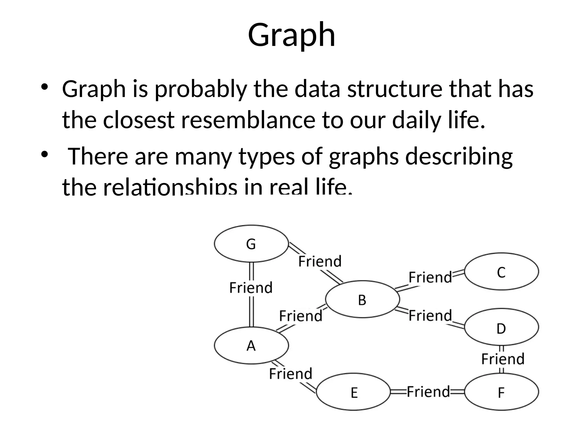
Graph
• Graph isprobably the data structure that has
the closest resemblance to our daily life.
• There are many types of graphs describing
the relationships in real life.
6.
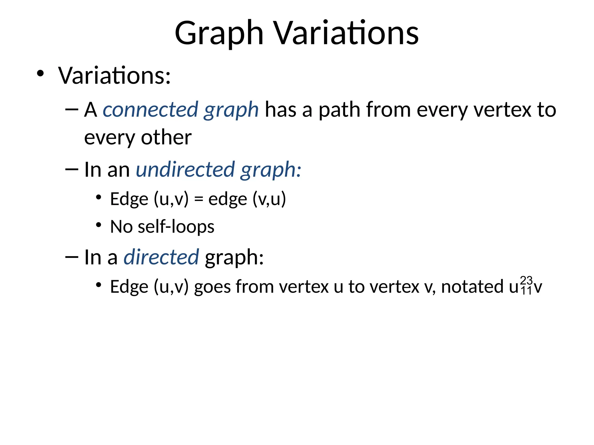
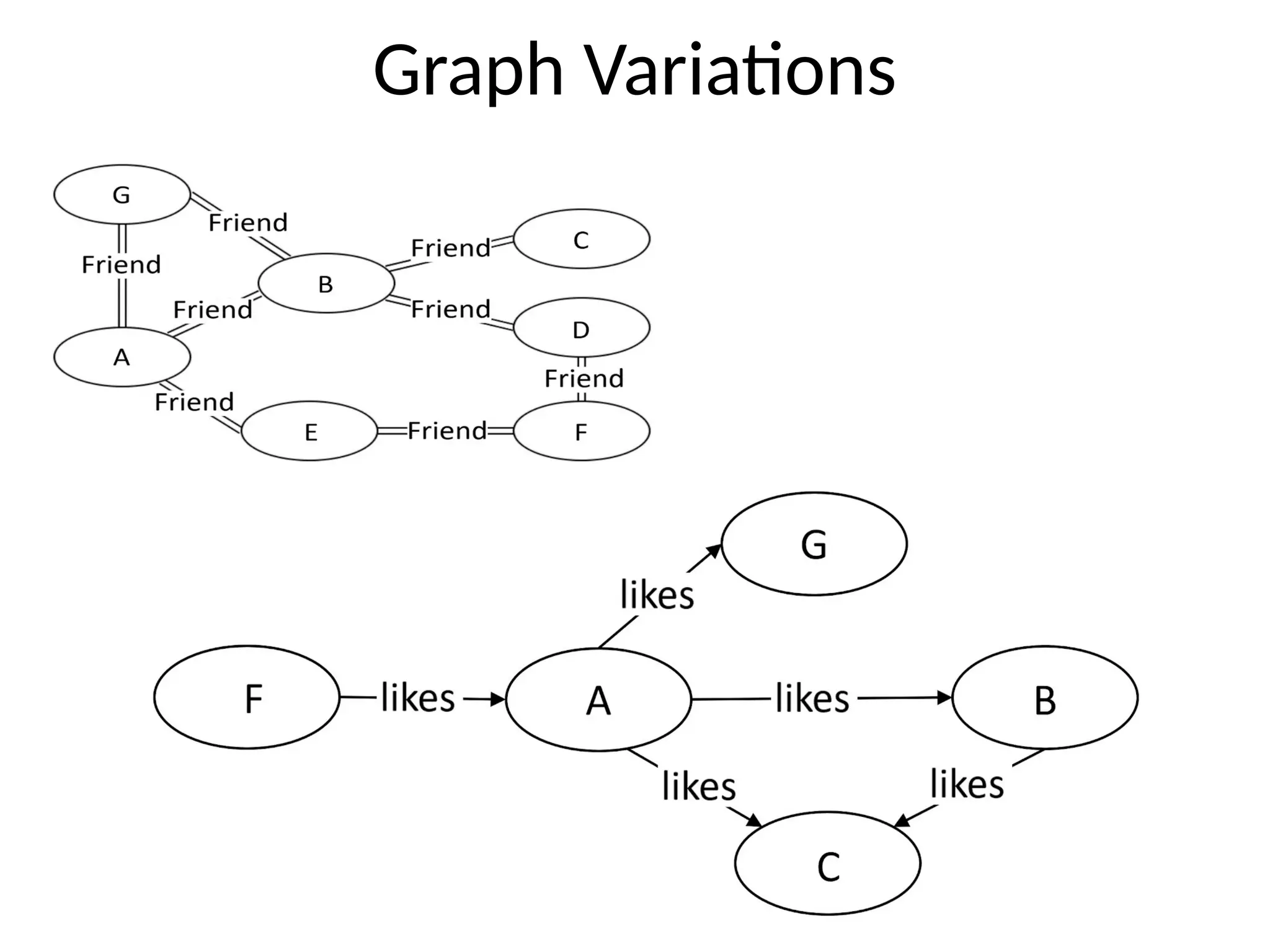
Graph Variations
• Variations:
–A connected graph has a path from every vertex to
every other
– In an undirected graph:
• Edge (u,v) = edge (v,u)
• No self-loops
– In a directed graph:
• Edge (u,v) goes from vertex u to vertex v, notated uv
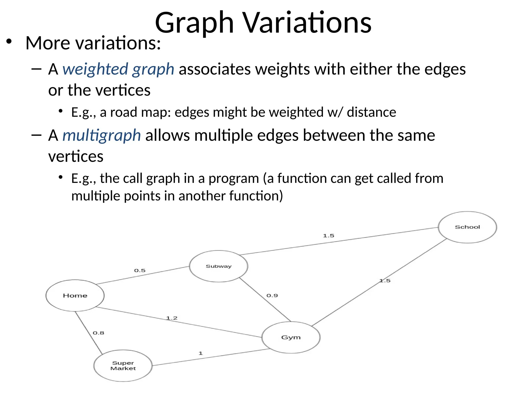
Graph Variations
• Morevariations:
– A weighted graph associates weights with either the edges
or the vertices
• E.g., a road map: edges might be weighted w/ distance
– A multigraph allows multiple edges between the same
vertices
• E.g., the call graph in a program (a function can get called from
multiple points in another function)
9.
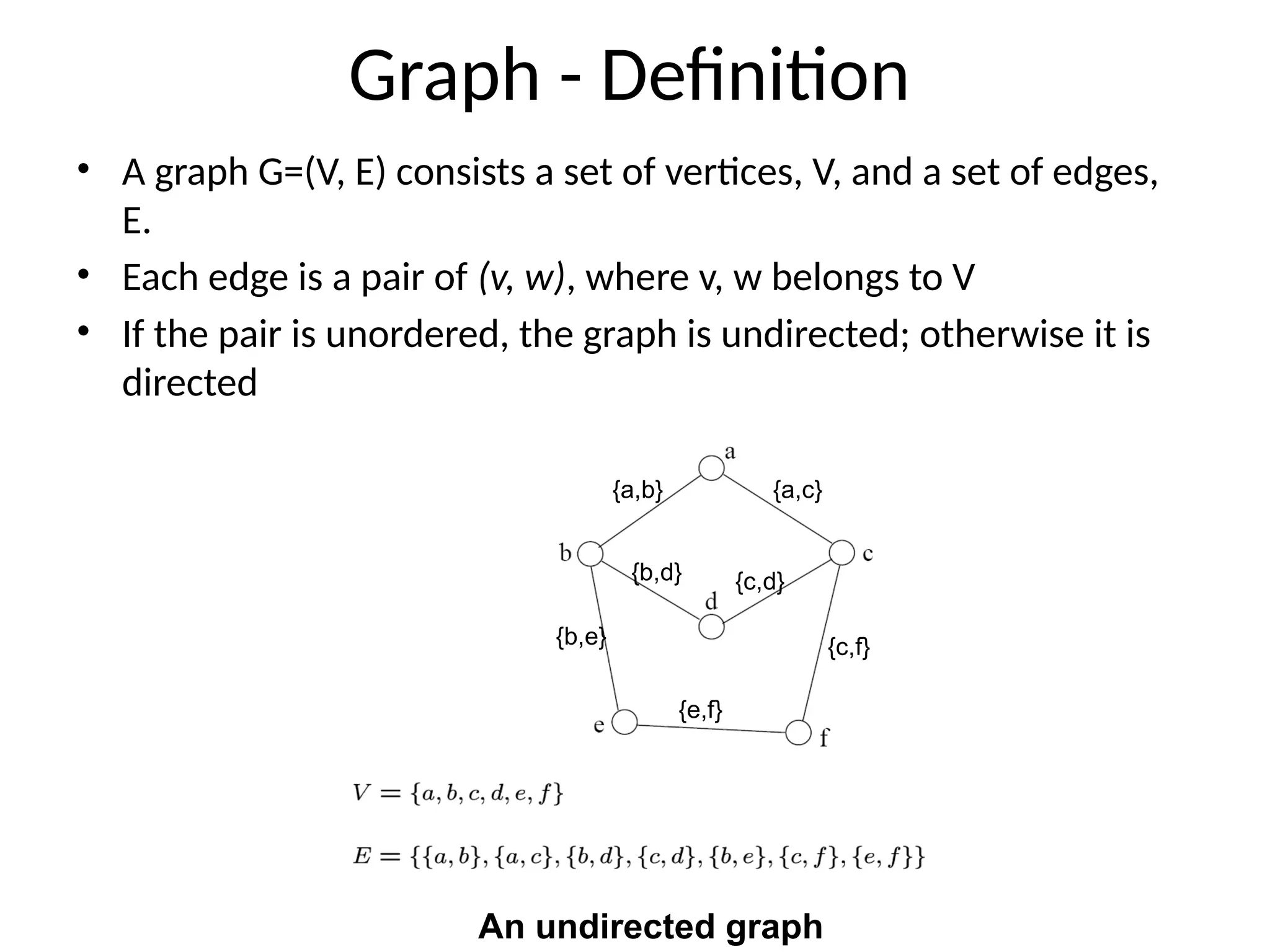
Graph - Definition
•A graph G=(V, E) consists a set of vertices, V, and a set of edges,
E.
• Each edge is a pair of (v, w), where v, w belongs to V
• If the pair is unordered, the graph is undirected; otherwise it is
directed
{c,f}
{a,c}
{a,b}
{b,d} {c,d}
{e,f}
{b,e}
An undirected graph
10.
Definition
• Path: thesequence of vertices to go through from one vertex to
another.
– a path from A to C is [A, B, C], or [A, G, B, C], or [A, E, F, D, B, C].
• Path Length: the number of edges in a path.
• Cycle: a path where the starting point and endpoint are the same
vertex.
– [A, B, D, F, E] forms a cycle. Similarly, [A, G, B] forms another cycle.
11.
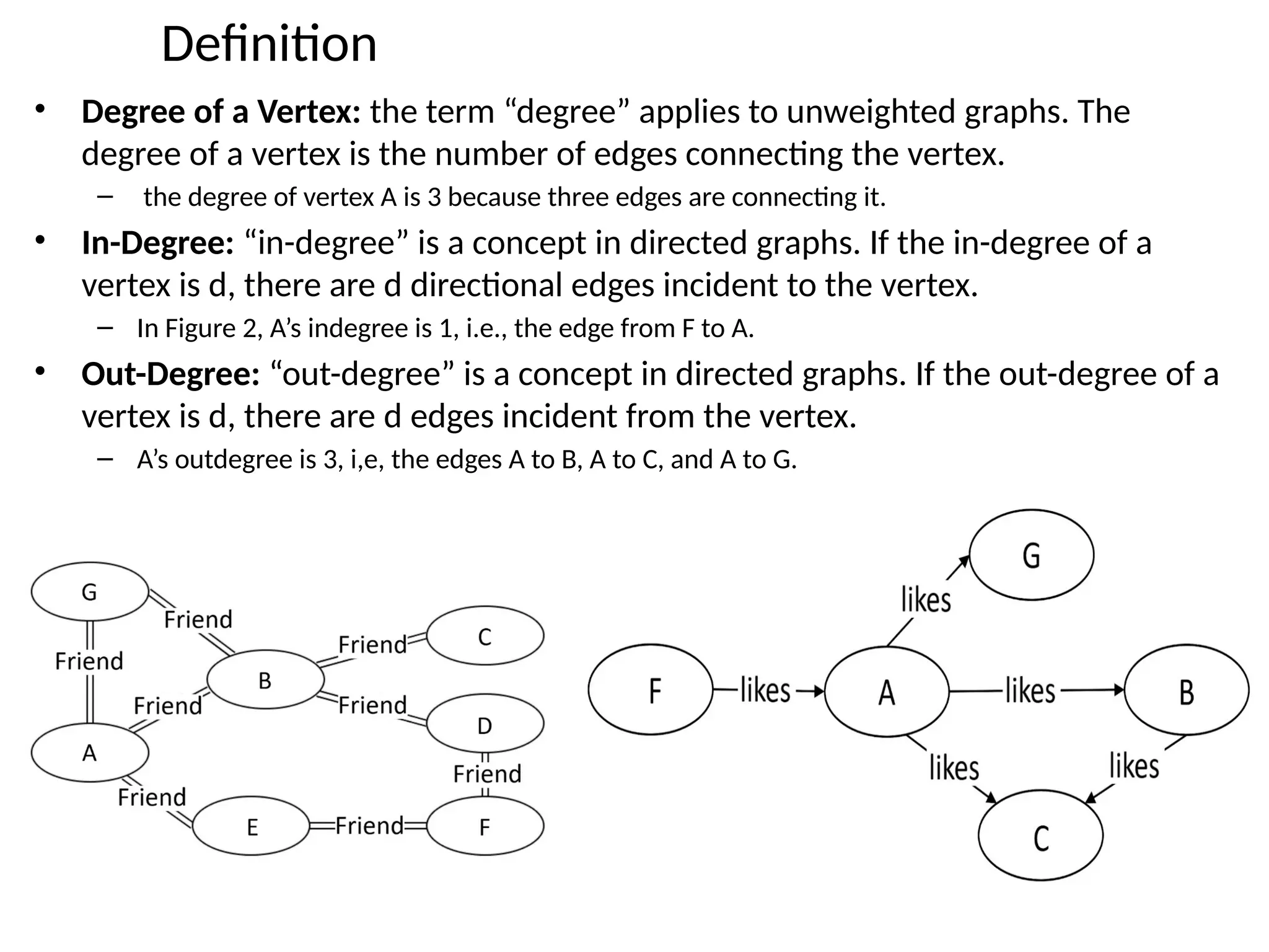
Definition
• Degree ofa Vertex: the term “degree” applies to unweighted graphs. The
degree of a vertex is the number of edges connecting the vertex.
– the degree of vertex A is 3 because three edges are connecting it.
• In-Degree: “in-degree” is a concept in directed graphs. If the in-degree of a
vertex is d, there are d directional edges incident to the vertex.
– In Figure 2, A’s indegree is 1, i.e., the edge from F to A.
• Out-Degree: “out-degree” is a concept in directed graphs. If the out-degree of a
vertex is d, there are d edges incident from the vertex.
– A’s outdegree is 3, i,e, the edges A to B, A to C, and A to G.
12.
Definition
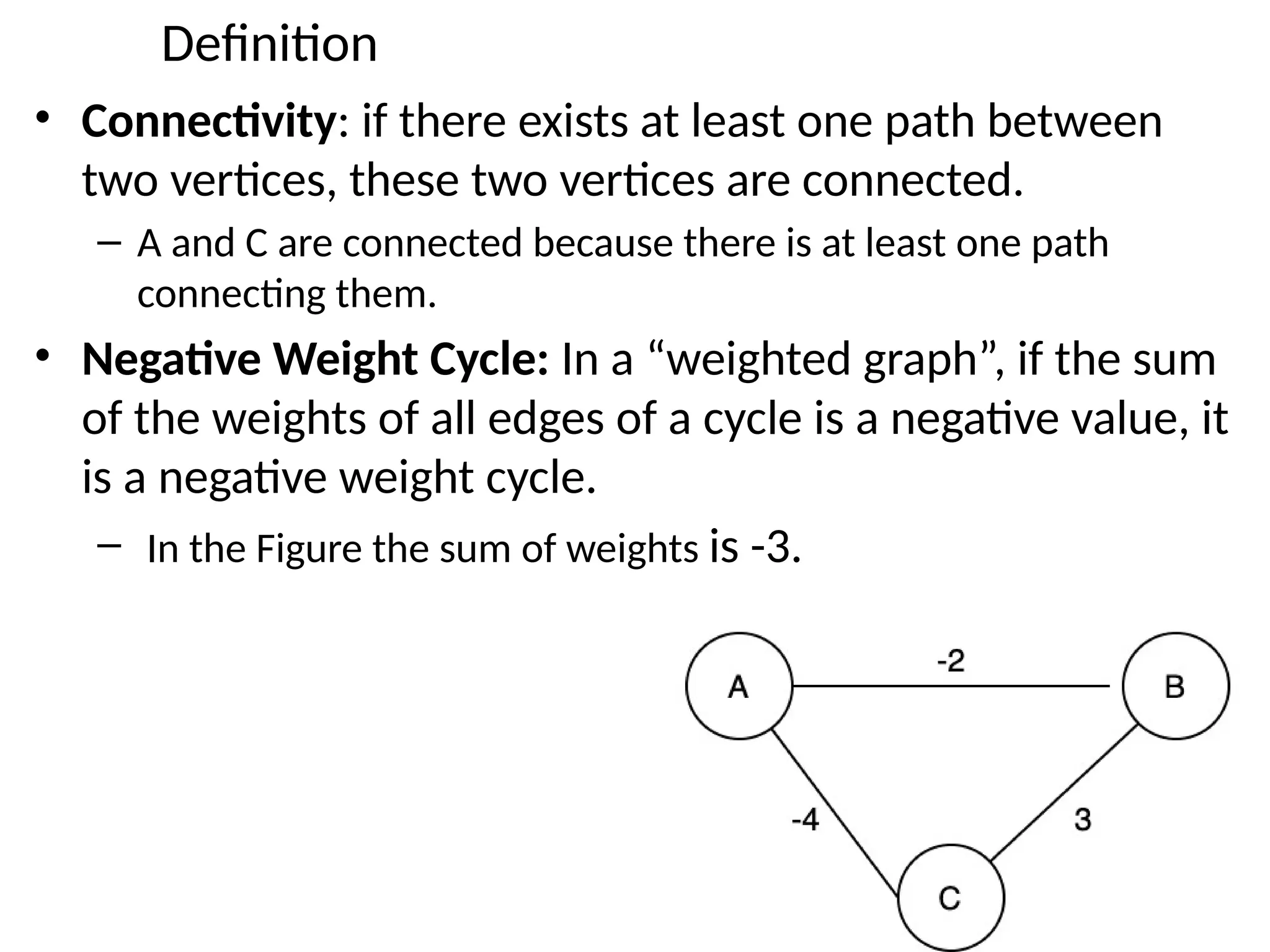
• Connectivity: ifthere exists at least one path between
two vertices, these two vertices are connected.
– A and C are connected because there is at least one path
connecting them.
• Negative Weight Cycle: In a “weighted graph”, if the sum
of the weights of all edges of a cycle is a negative value, it
is a negative weight cycle.
– In the Figure the sum of weights is -3.
13.
Definition
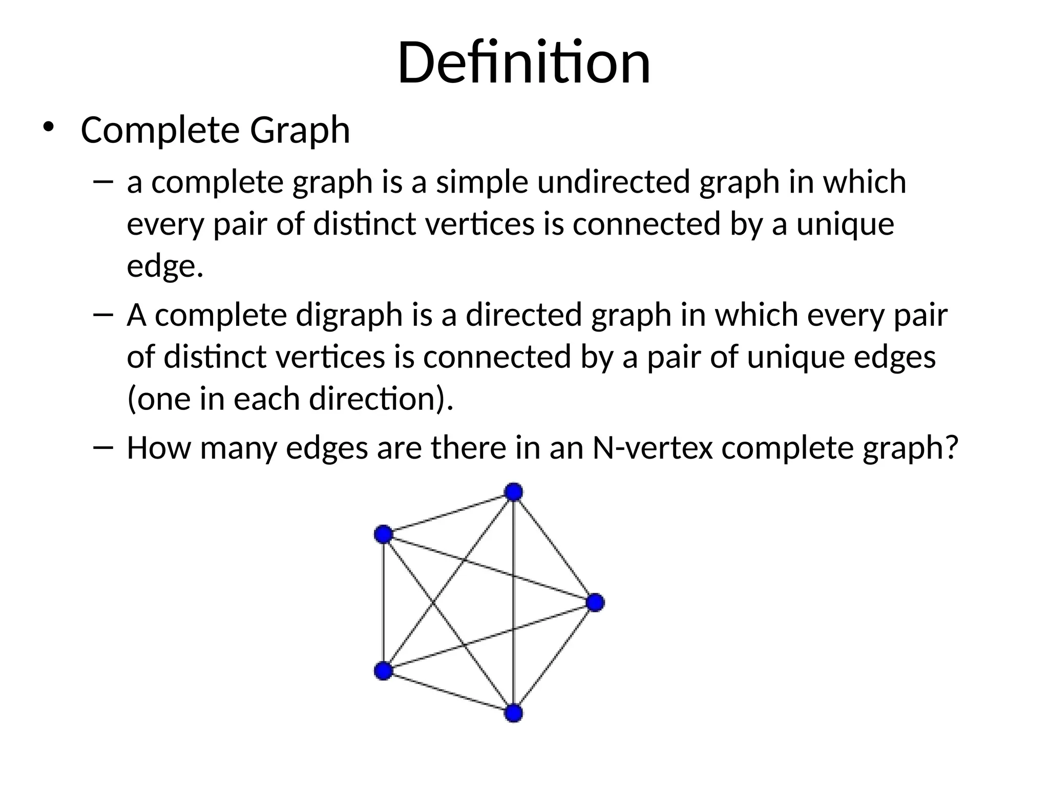
• Complete Graph
–a complete graph is a simple undirected graph in which
every pair of distinct vertices is connected by a unique
edge.
– A complete digraph is a directed graph in which every pair
of distinct vertices is connected by a pair of unique edges
(one in each direction).
– How many edges are there in an N-vertex complete graph?
14.
Definition
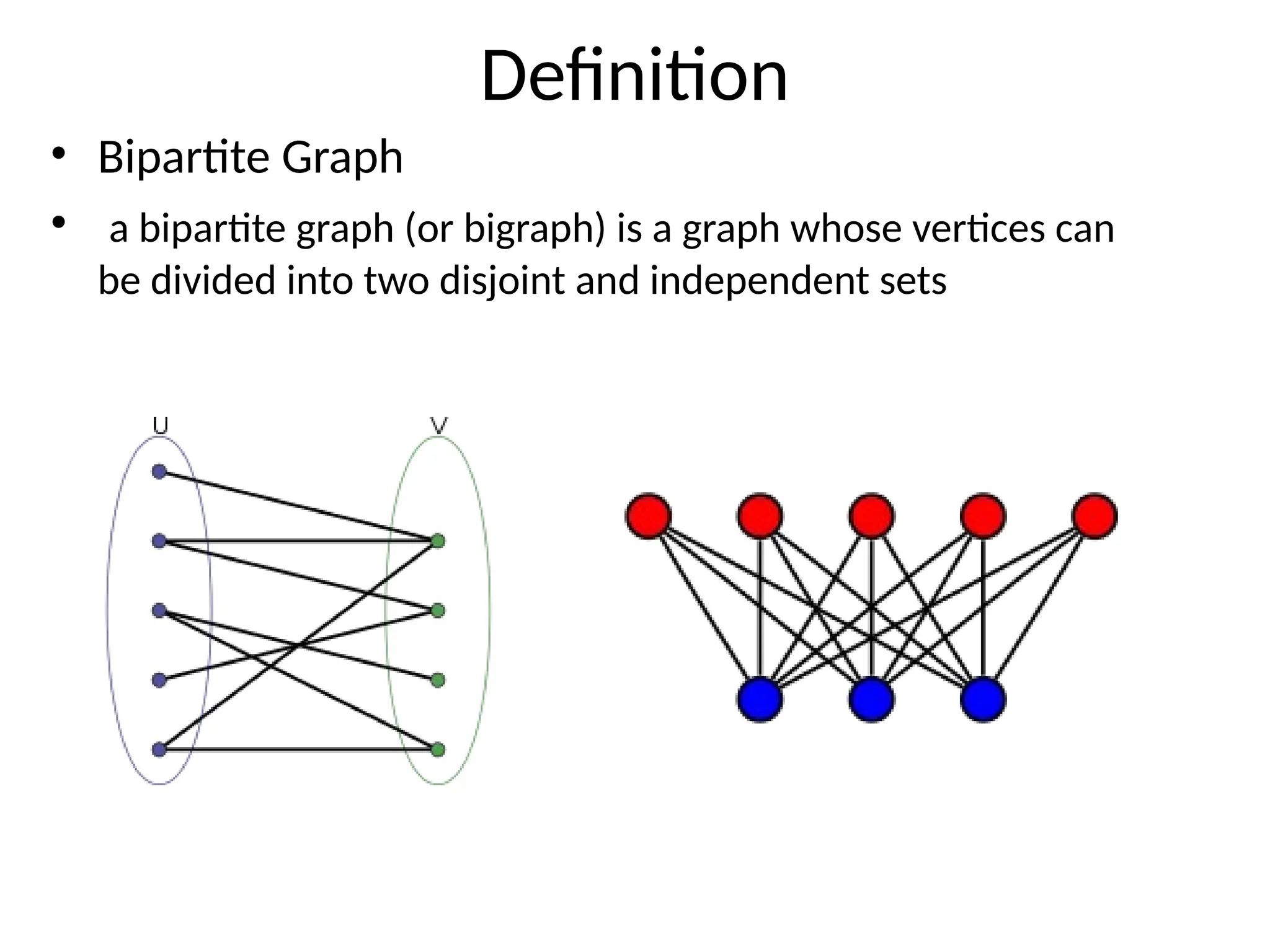
• Bipartite Graph
•a bipartite graph (or bigraph) is a graph whose vertices can
be divided into two disjoint and independent sets
15.
Definition
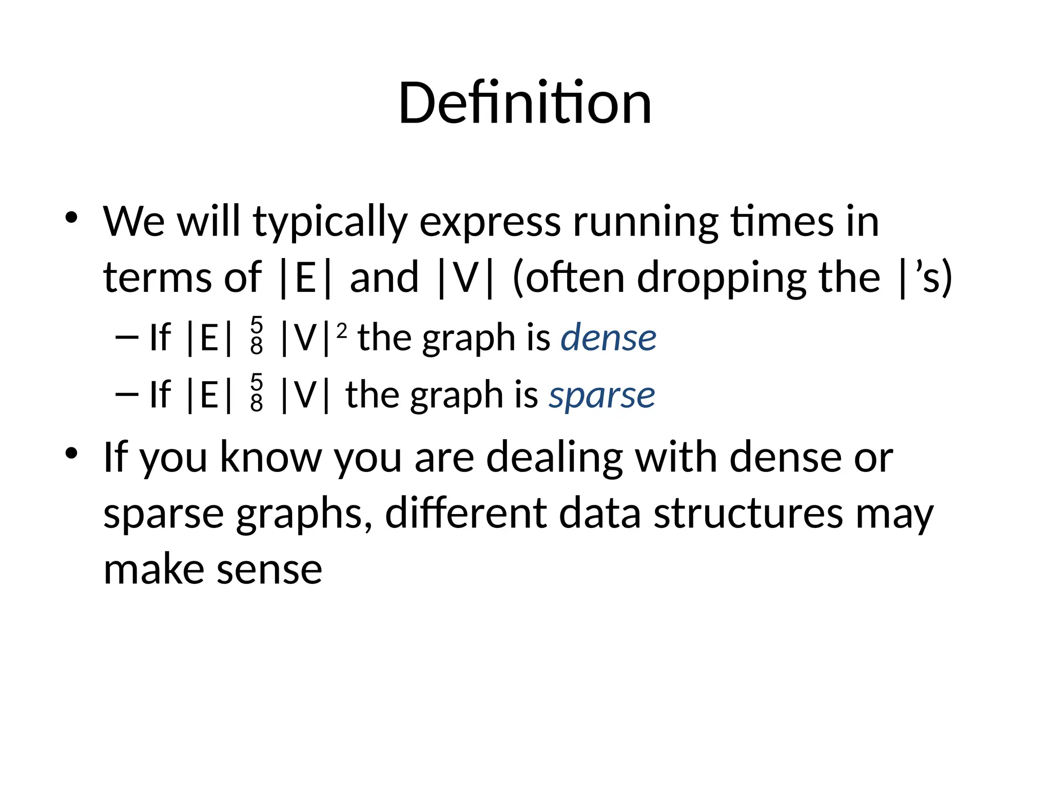
• We willtypically express running times in
terms of |E| and |V| (often dropping the |’s)
– If |E| |V|2
the graph is dense
– If |E| |V| the graph is sparse
• If you know you are dealing with dense or
sparse graphs, different data structures may
make sense
16.
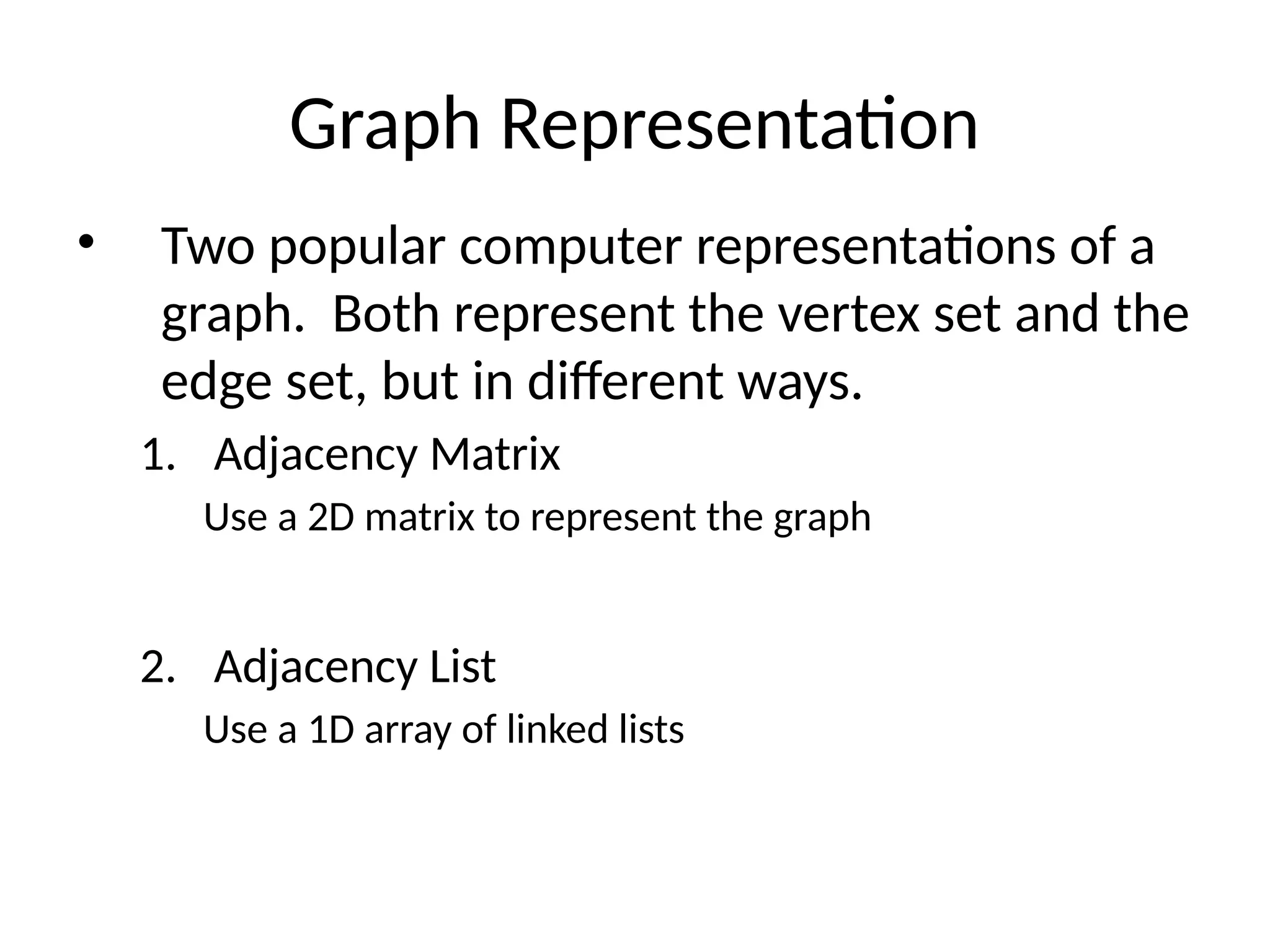
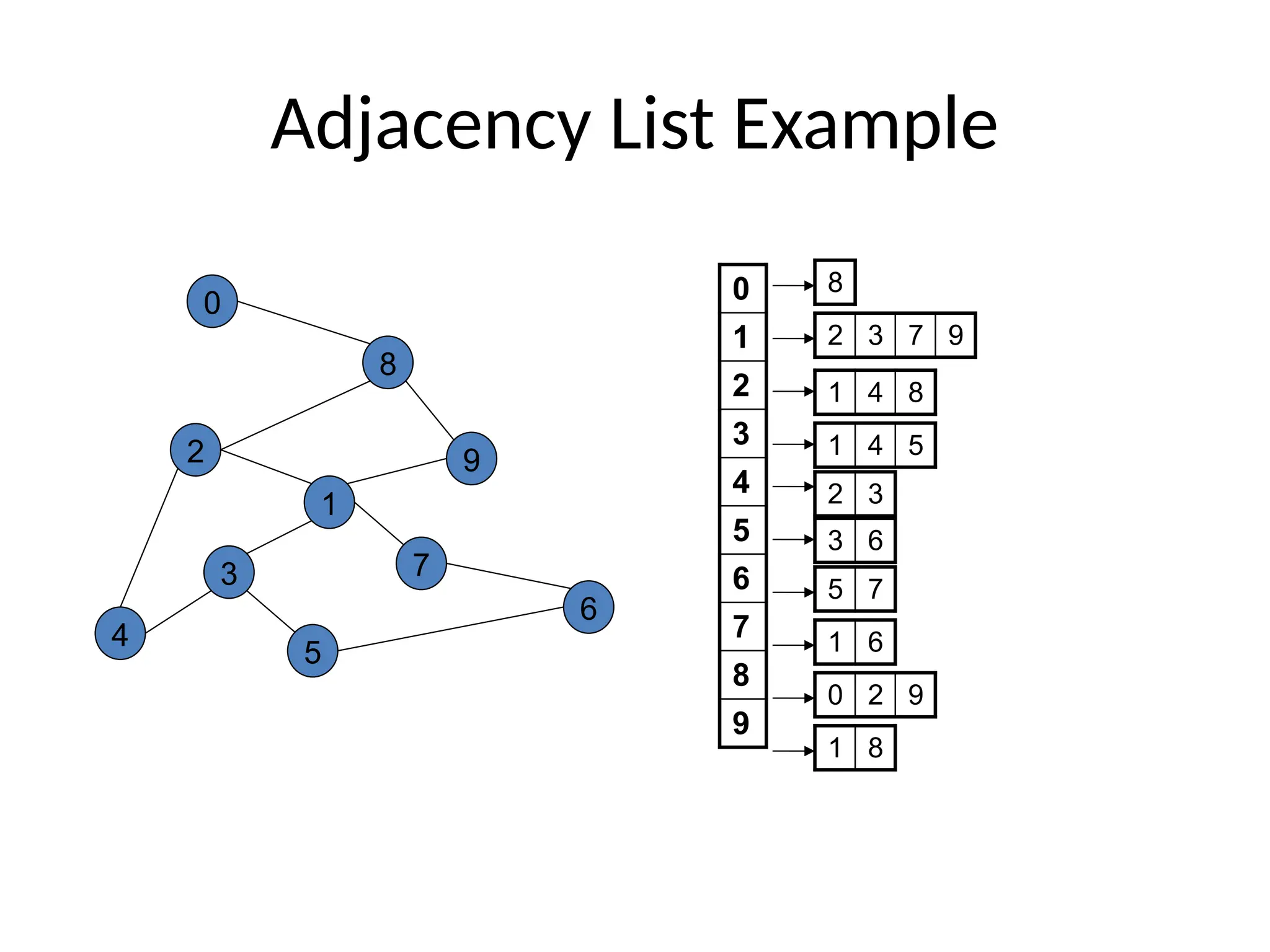
Graph Representation
• Twopopular computer representations of a
graph. Both represent the vertex set and the
edge set, but in different ways.
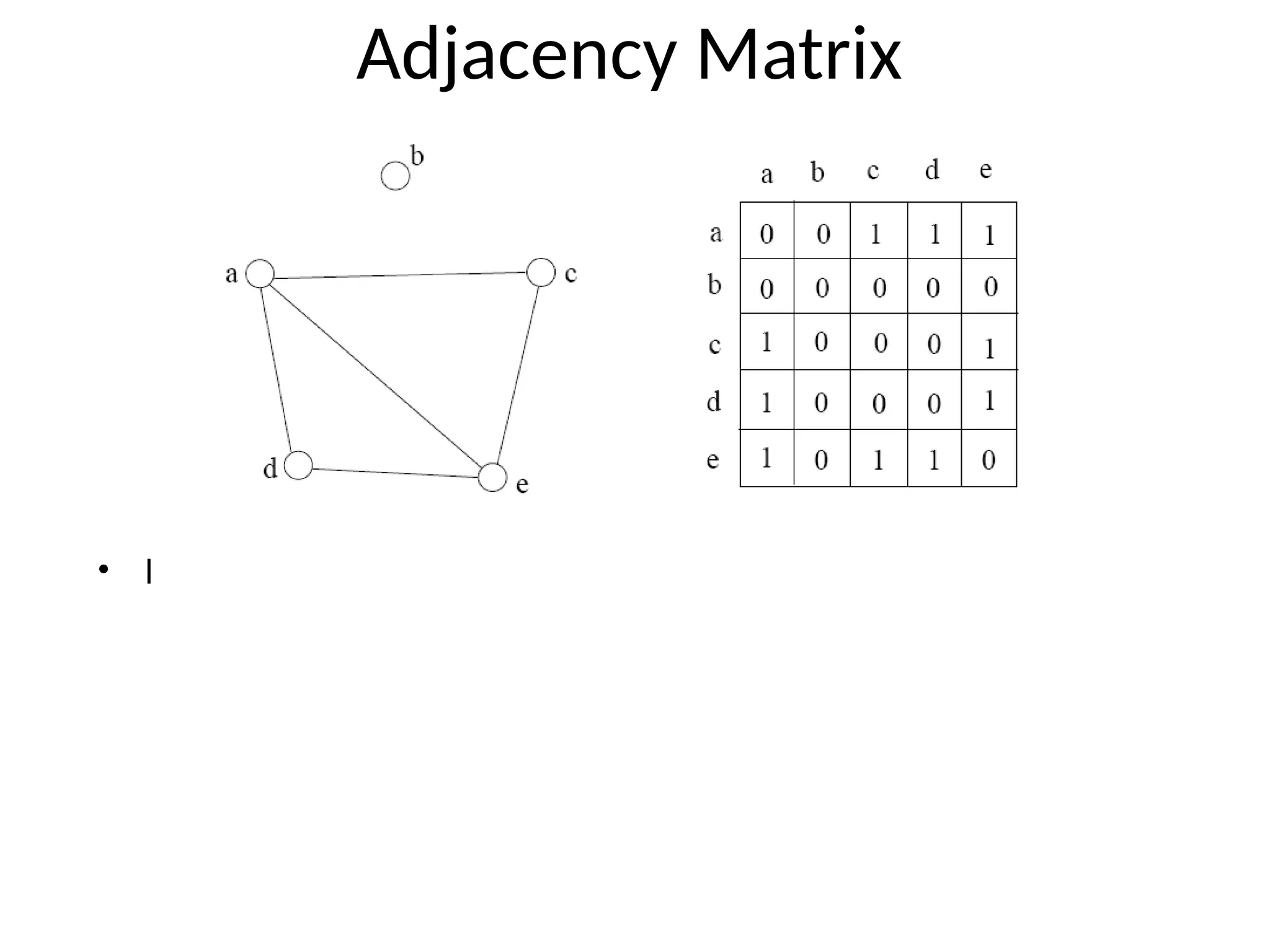
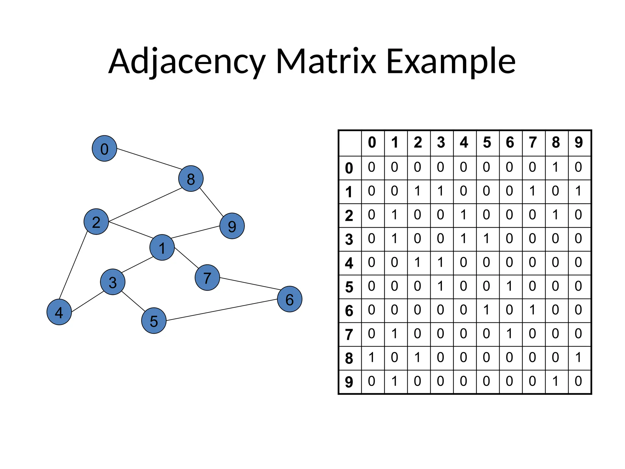
1. Adjacency Matrix
Use a 2D matrix to represent the graph
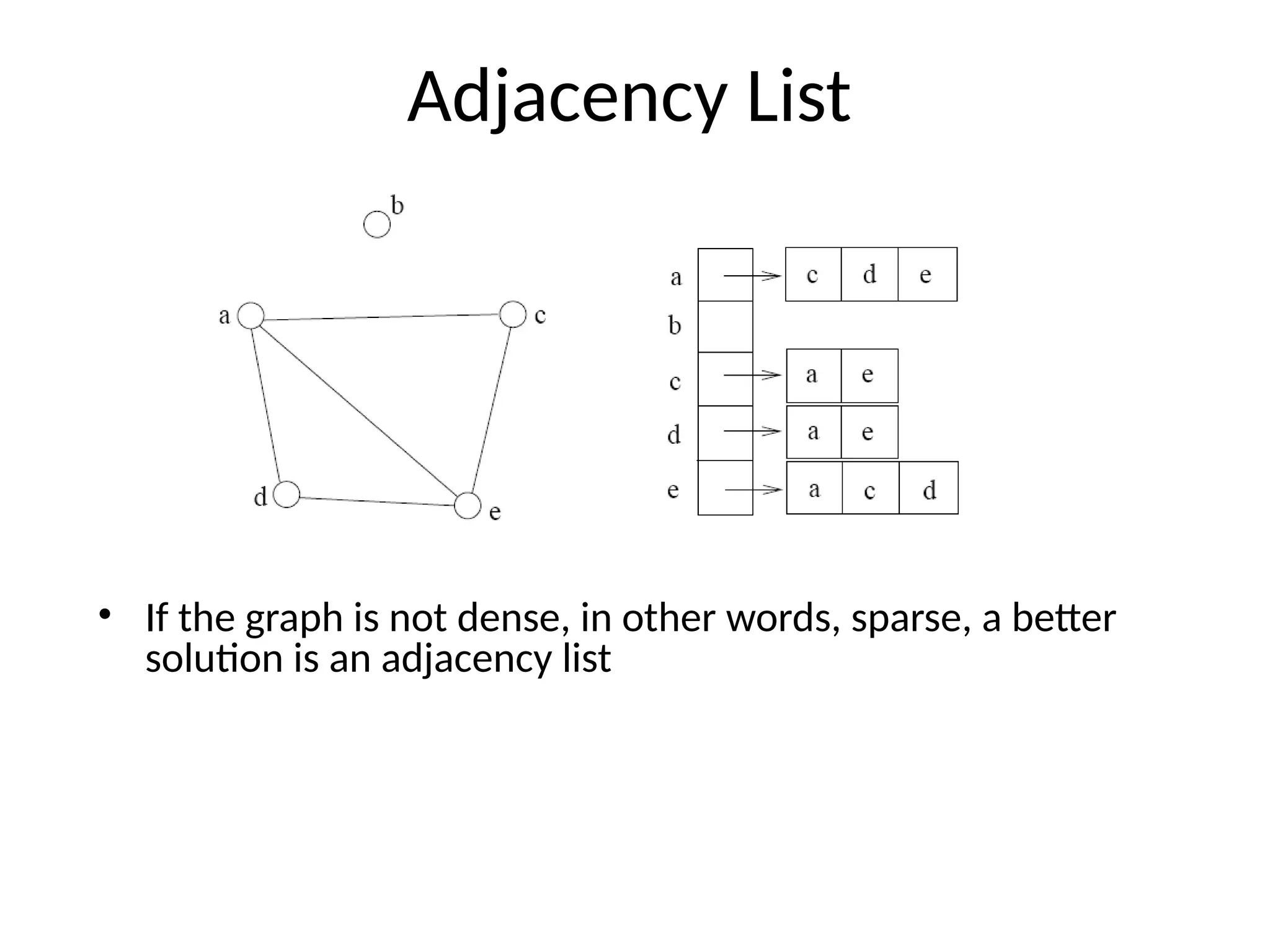
2. Adjacency List
Use a 1D array of linked lists
Adjacency List vs.Matrix
• Adjacency List
– More compact than adjacency matrices if graph has few
edges
– Requires more time to find if an edge exists
• Adjacency Matrix
– Always require n2
space
• This can waste a lot of space if the number of edges are
sparse
– Can quickly find if an edge exists
22.
Graph Traversal
• Applicationexample
– Given a graph representation and a vertex s in the
graph
– Find paths from s to other vertices
• Two common graph traversal algorithms
• Breadth-First Search (BFS)
– Find the shortest paths in an unweighted graph
• Depth-First Search (DFS)
– Topological sort
– Find strongly connected components
23.
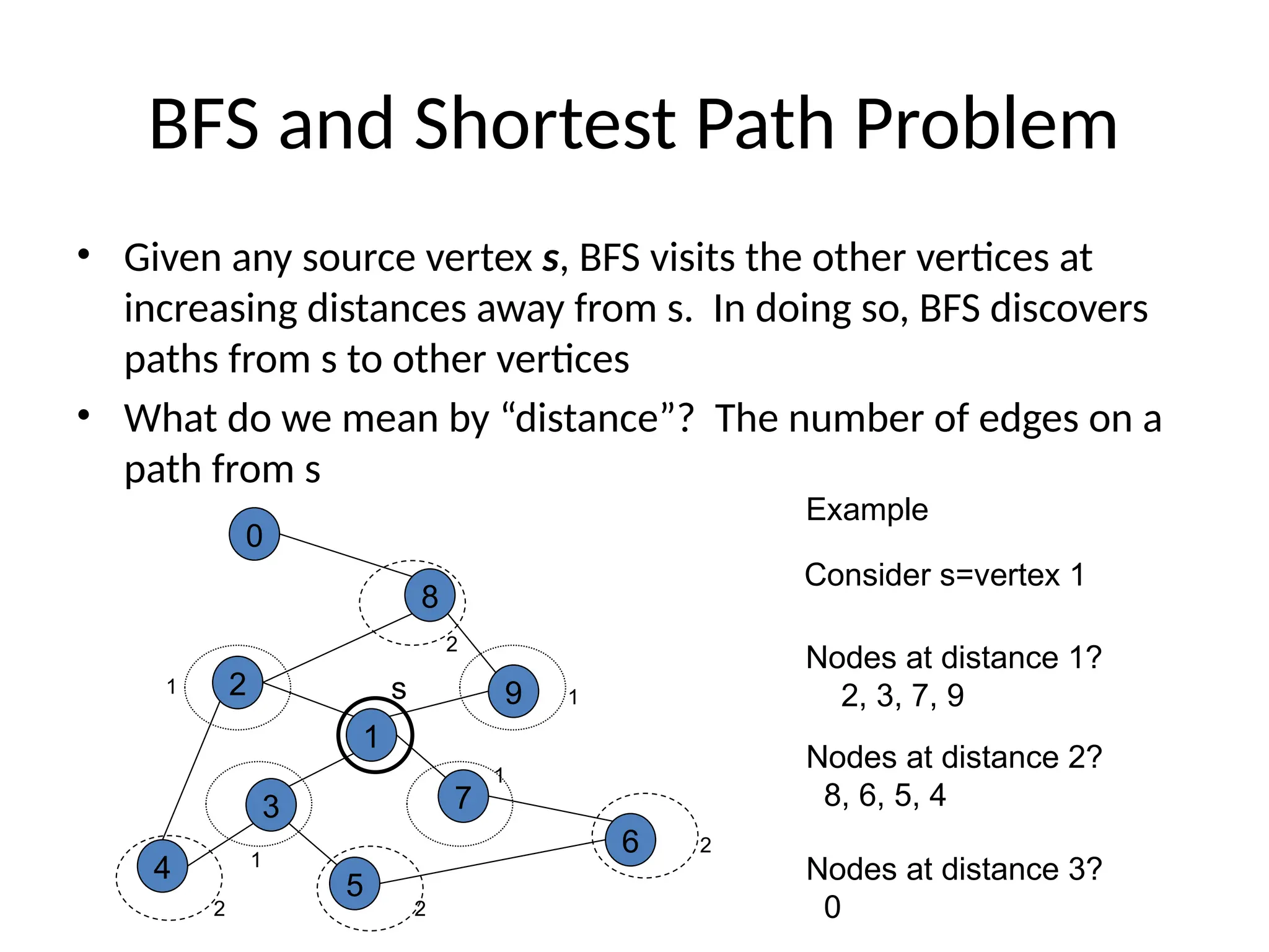
BFS and ShortestPath Problem
• Given any source vertex s, BFS visits the other vertices at
increasing distances away from s. In doing so, BFS discovers
paths from s to other vertices
• What do we mean by “distance”? The number of edges on a
path from s
2
4
3
5
1
7
6
9
8
0
Consider s=vertex 1
Nodes at distance 1?
2, 3, 7, 9
1
1
1
1
2
2
2
2
s
Example
Nodes at distance 2?
8, 6, 5, 4
Nodes at distance 3?
0
24.
Graph Searching
• Given:a graph G = (V, E), directed or undirected
• Goal: methodically explore every vertex and
every edge
• Ultimately: build a tree on the graph
– Pick a vertex as the root
– Choose certain edges to produce a tree
– Note: might also build a forest if graph is not
connected
25.
Breadth-First Search
• “Explore”a graph, turning it into a tree
– One vertex at a time
– Expand frontier of explored vertices across the
breadth of the frontier
• Builds a tree over the graph
– Pick a source vertex to be the root
– Find (“discover”) its children, then their children,
etc.
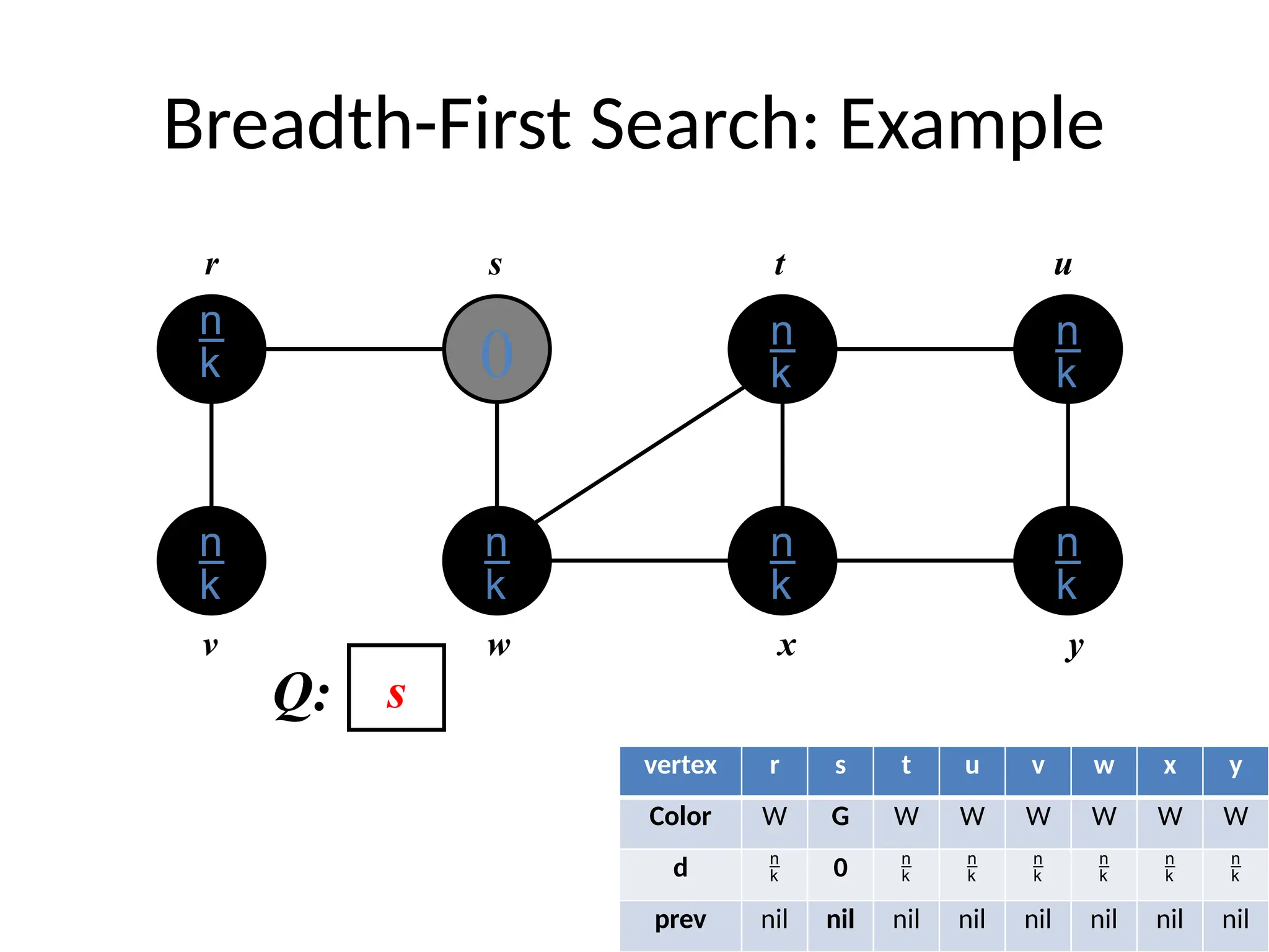
26.
Breadth-First Search
• Everyvertex of a graph contains a color at every
moment:
– White vertices have not been discovered
• All vertices start with white initially
– Grey vertices are discovered but not fully explored
• They may be adjacent to white vertices
– Black vertices are discovered and fully explored
• They are adjacent only to black and gray vertices
• Explore vertices by scanning adjacency list of grey
vertices
27.
Breadth-First Search: TheCode
Data: color[V], prev[V],d[V]
BFS(G) // starts from here
{
for each vertex u V-
{s}
{
color[u]=WHITE;
prev[u]=NIL;
d[u]=inf;
}
color[s]=GRAY;
d[s]=0; prev[s]=NIL;
Q=empty;
ENQUEUE(Q,s);
While(Q not empty)
{
u = DEQUEUE(Q);
for each v adj[u]{
if (color[v] == WHITE){
color[v] = GREY;
d[v] = d[u] + 1;
prev[v] = u;
Enqueue(Q, v);
}
}
color[u] = BLACK;
}
}
BFS: Complexity
Data: color[V],prev[V],d[V]
BFS(G) // starts from here
{
for each vertex u V-
{s}
{
color[u]=WHITE;
prev[u]=NIL;
d[u]=inf;
}
color[s]=GRAY;
d[s]=0; prev[s]=NIL;
Q=empty;
ENQUEUE(Q,s);
While(Q not empty)
{
u = DEQUEUE(Q);
for each v adj[u]{
if(color[v] == WHITE){
color[v] = GREY;
d[v] = d[u] + 1;
prev[v] = u;
Enqueue(Q, v);
}
}
color[u] = BLACK;
}
}
O(V)
O(V)
u = every vertex, but only once
(Why?)
What will be the running time?
Total running time: O(V+E)
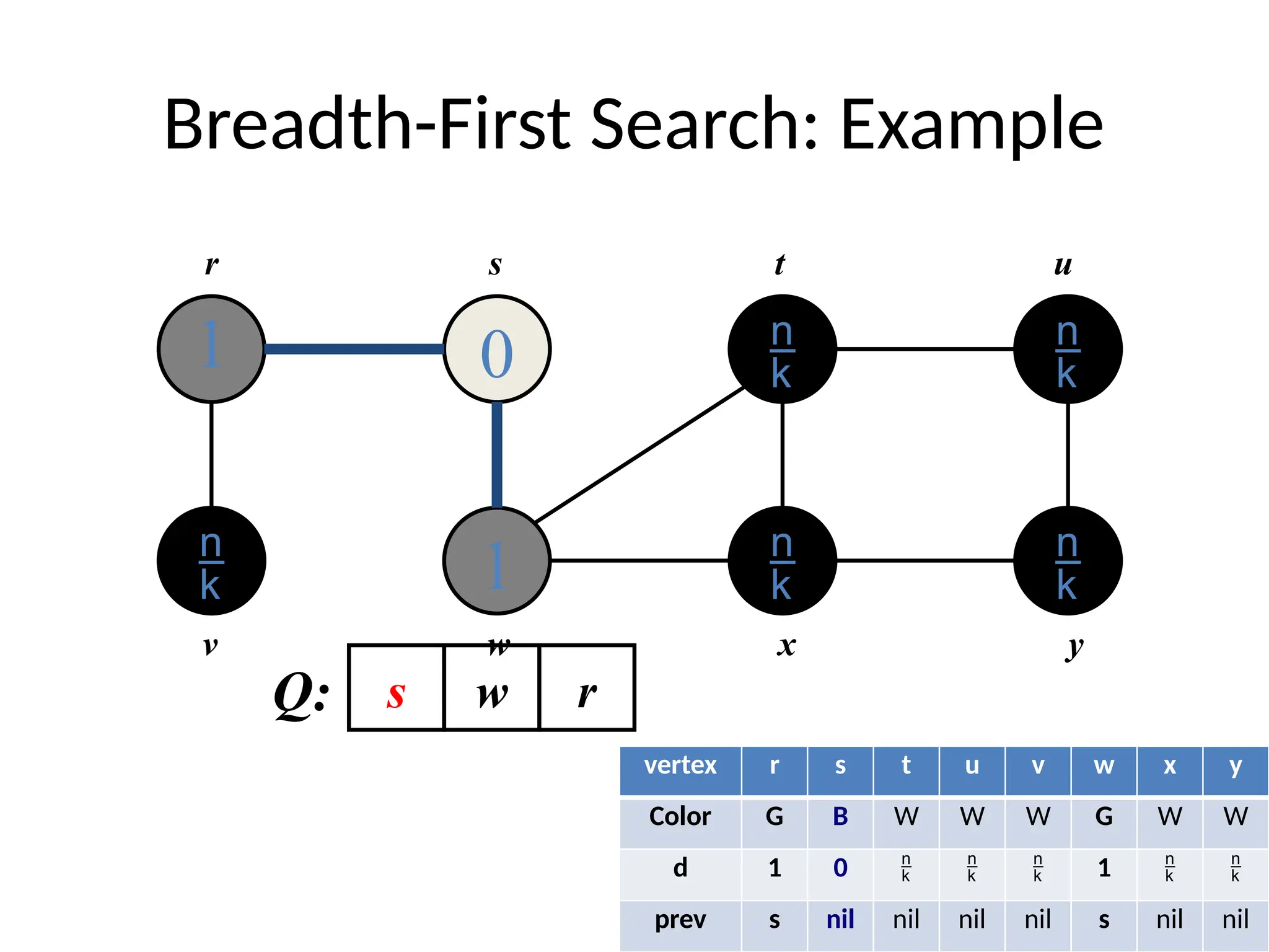
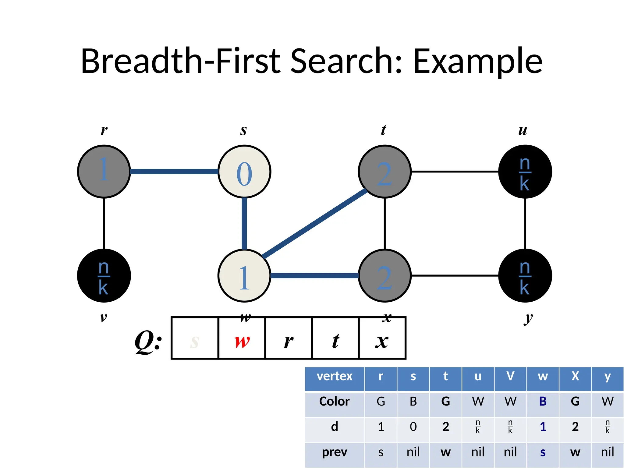
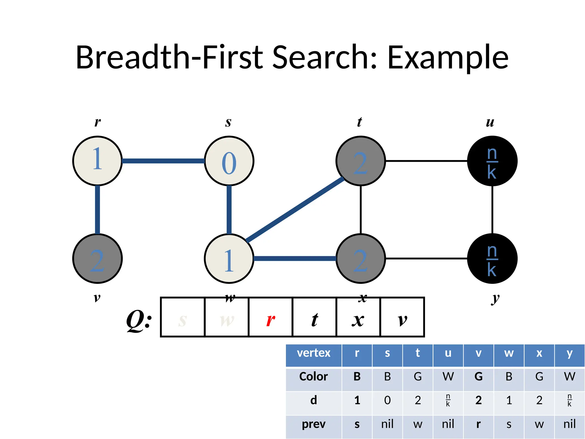
41.
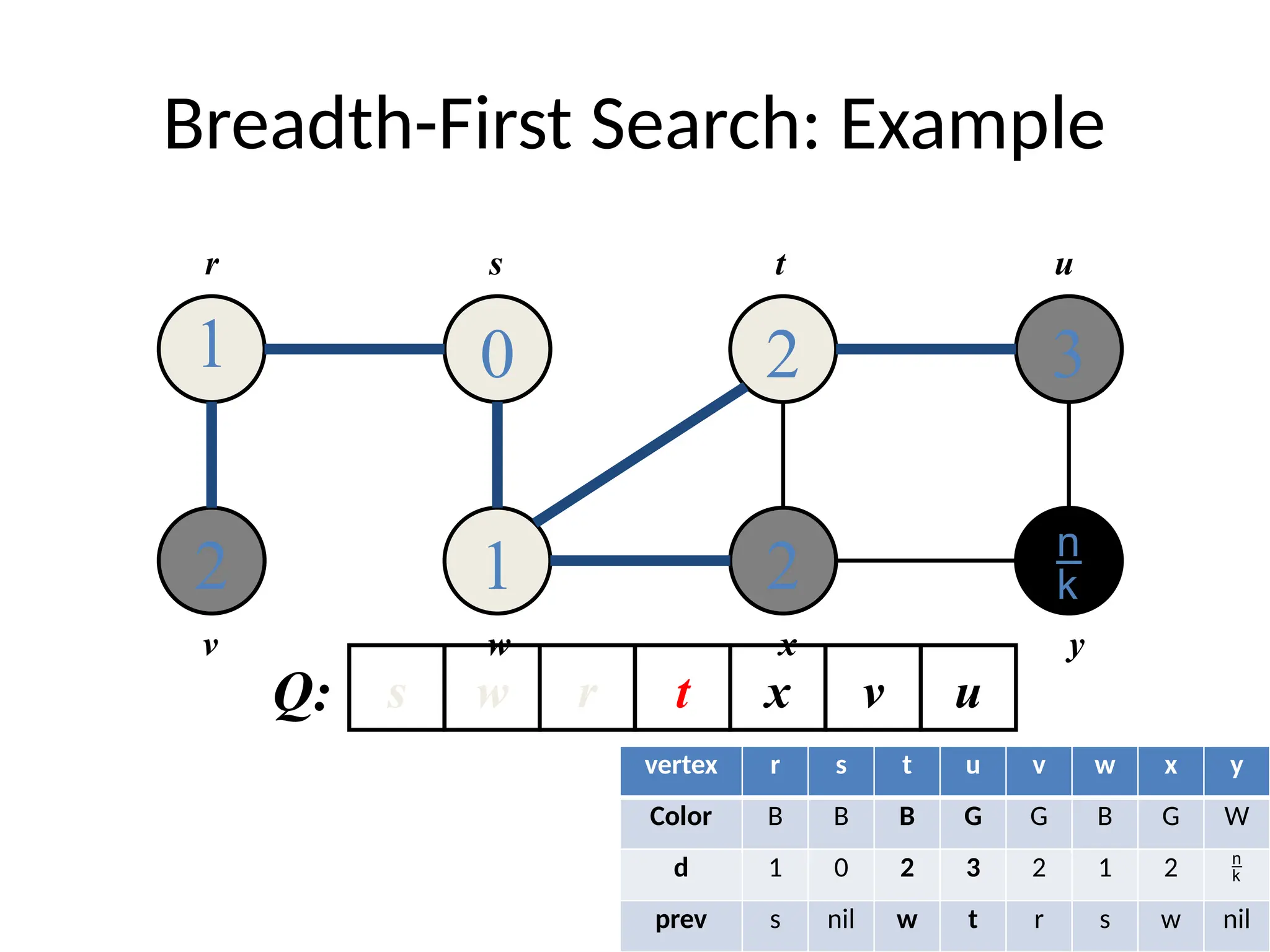
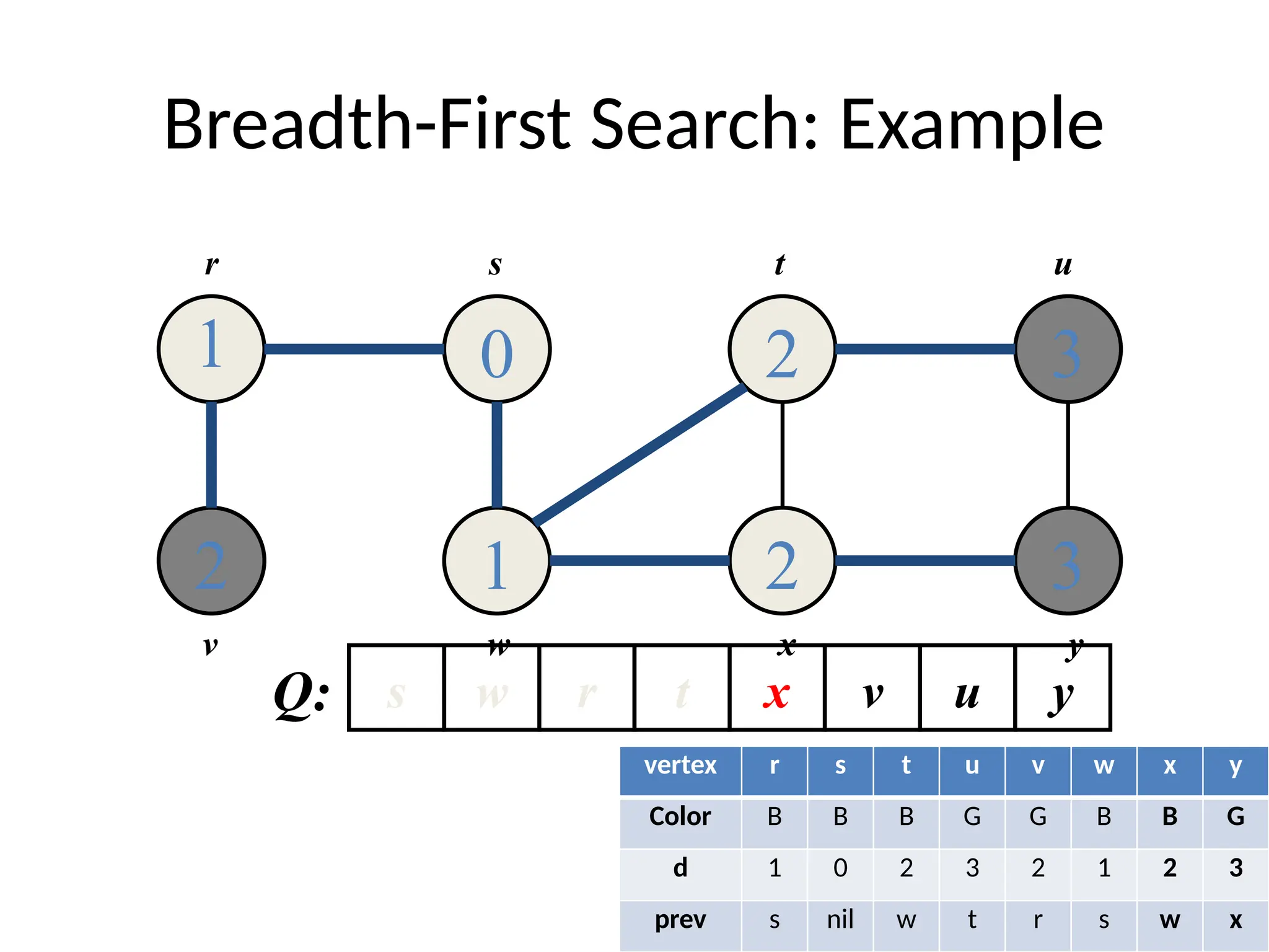
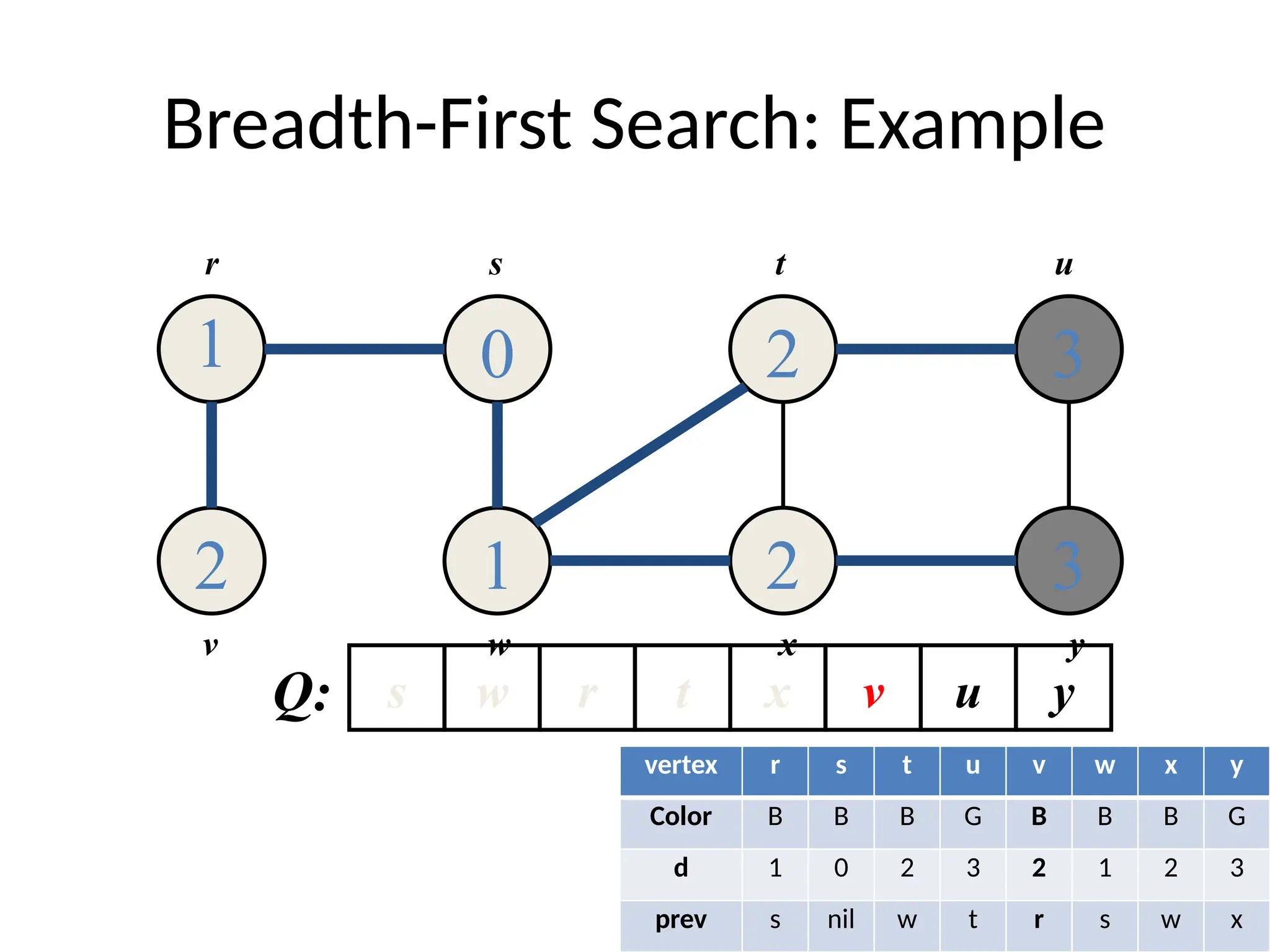
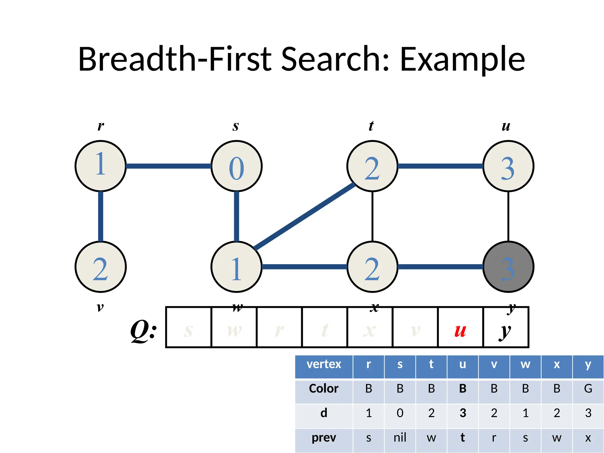
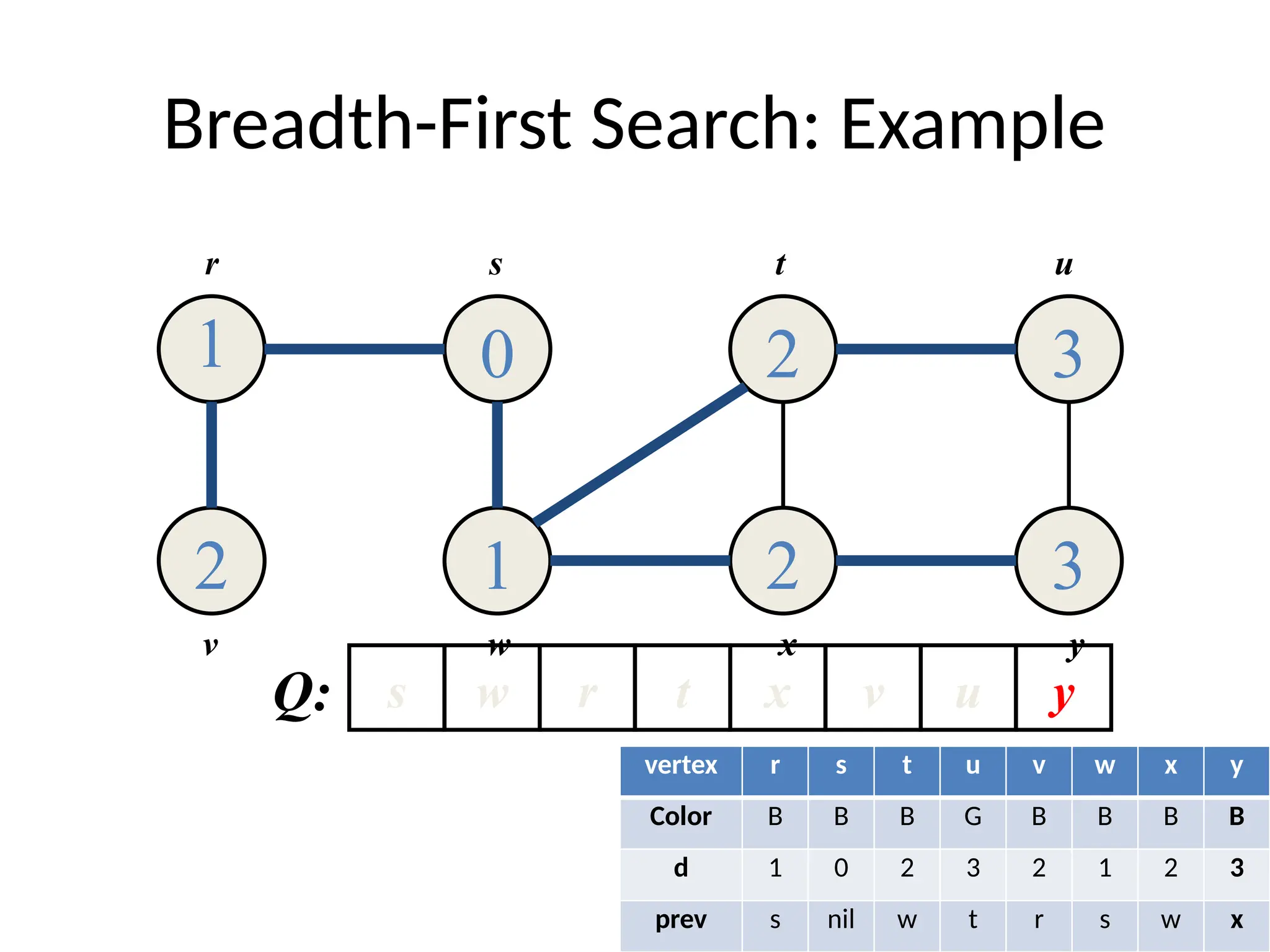
Breadth-First Search: Properties
•BFS calculates the shortest-path distance to the
source node
– Shortest-path distance (s,v) = minimum number of
edges from s to v, or if v not reachable from s
– Proof given in the book (p. 472-5)
• BFS builds breadth-first tree, in which paths to root
represent shortest paths in G
– Thus can use BFS to calculate shortest path from one
vertex to another in O(V+E) time
42.
Application of BFS
•Find the shortest path in an
undirected/directed unweighted graph.
• Find the bipartite-ness of a graph.
• Find cycle in a graph.
• Find the connectedness of a graph.
• And many more.
43.
Exercises on BFS
•CLRS – Chapter 22 – elementary Graph
Algorithms
• Exercise you have to solve: (Page 602)
– 22.2-7 (Wrestler)
– 22.2-8 (Diameter)
– 22.2-9 (Traverse)
44.
Depth-First Search
• Input:
–G = (V, E) (No source vertex given!)
• Goal:
– Explore the edges of G to “discover” every vertex in V starting at the most
current visited node
– Search may be repeated from multiple sources
• Output:
– 2 timestamps on each vertex:
• d[v] = discovery time
• f[v] = finishing time (done with examining v’s adjacency list)
– Depth-first forest
1 2
5 4
3
45.
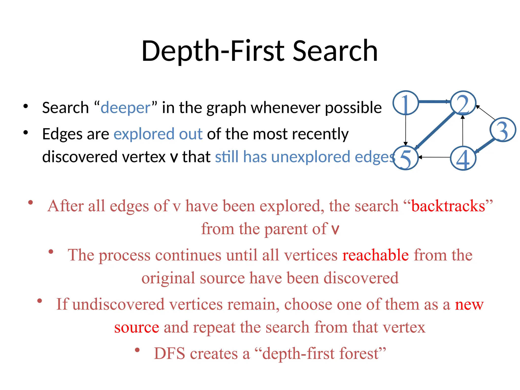
Depth-First Search
• Search“deeper” in the graph whenever possible
• Edges are explored out of the most recently
discovered vertex v that still has unexplored edges
• After all edges of v have been explored, the search “backtracks”
from the parent of v
• The process continues until all vertices reachable from the
original source have been discovered
• If undiscovered vertices remain, choose one of them as a new
source and repeat the search from that vertex
• DFS creates a “depth-first forest”
1 2
5 4
3
46.
DFS Additional DataStructures
• Global variable: time-stamp
– Incremented when nodes are discovered or finished
• color[u] – similar to BFS
– White before discovery, gray while processing and black
when finished processing
• prev[u] – predecessor of u
• d[u], f[u] – discovery and finish times
GRAY
WHITE BLACK
0 2V
d[u] f[u]
1 ≤ d[u] < f [u] ≤ 2 |V|
47.
Depth-First Search: TheCode
Data: color[V], time,
prev[V],d[V], f[V]
DFS(G) // where prog starts
{
for each vertex u V
{
color[u] = WHITE;
prev[u]=NIL;
f[u]=inf;
d[u]=inf;
}
time = 0;
for each vertex u V
if (color[u] == WHITE)
DFS_Visit(u);
}
DFS_Visit(u)
{
color[u] = GREY;
time = time+1;
d[u] = time;
for each v Adj[u]
{
if(color[v] == WHITE){
prev[v]=u;
DFS_Visit(v);}
}
color[u] = BLACK;
time = time+1;
f[u] = time;
}
Initialize
48.
Depth-First Search: TheCode
Data: color[V], time,
prev[V],d[V], f[V]
DFS(G) // where prog starts
{
for each vertex u V
{
color[u] = WHITE;
prev[u]=NIL;
f[u]=inf;
d[u]=inf;
}
time = 0;
for each vertex u V
if (color[u] == WHITE)
DFS_Visit(u);
}
DFS_Visit(u)
{
color[u] = GREY;
time = time+1;
d[u] = time;
for each v Adj[u]
{
if(color[v] == WHITE){
prev[v]=u;
DFS_Visit(v);}
}
color[u] = BLACK;
time = time+1;
f[u] = time;
}
What does d[u] represent?
49.
Depth-First Search: TheCode
Data: color[V], time,
prev[V],d[V], f[V]
DFS(G) // where prog starts
{
for each vertex u V
{
color[u] = WHITE;
prev[u]=NIL;
f[u]=inf;
d[u]=inf;
}
time = 0;
for each vertex u V
if (color[u] == WHITE)
DFS_Visit(u);
}
DFS_Visit(u)
{
color[u] = GREY;
time = time+1;
d[u] = time;
for each v Adj[u]
{
if(color[v] == WHITE){
prev[v]=u;
DFS_Visit(v);}
}
color[u] = BLACK;
time = time+1;
f[u] = time;
}
What does f[u] represent?
50.
Depth-First Search: TheCode
Data: color[V], time,
prev[V],d[V], f[V]
DFS(G) // where prog starts
{
for each vertex u V
{
color[u] = WHITE;
prev[u]=NIL;
f[u]=inf;
d[u]=inf;
}
time = 0;
for each vertex u V
if (color[u] == WHITE)
DFS_Visit(u);
}
DFS_Visit(u)
{
color[u] = GREY;
time = time+1;
d[u] = time;
for each v Adj[u]
{
if(color[v] == WHITE){
prev[v]=u;
DFS_Visit(v);
}}
color[u] = BLACK;
time = time+1;
f[u] = time;
}
Will all vertices eventually be colored black?
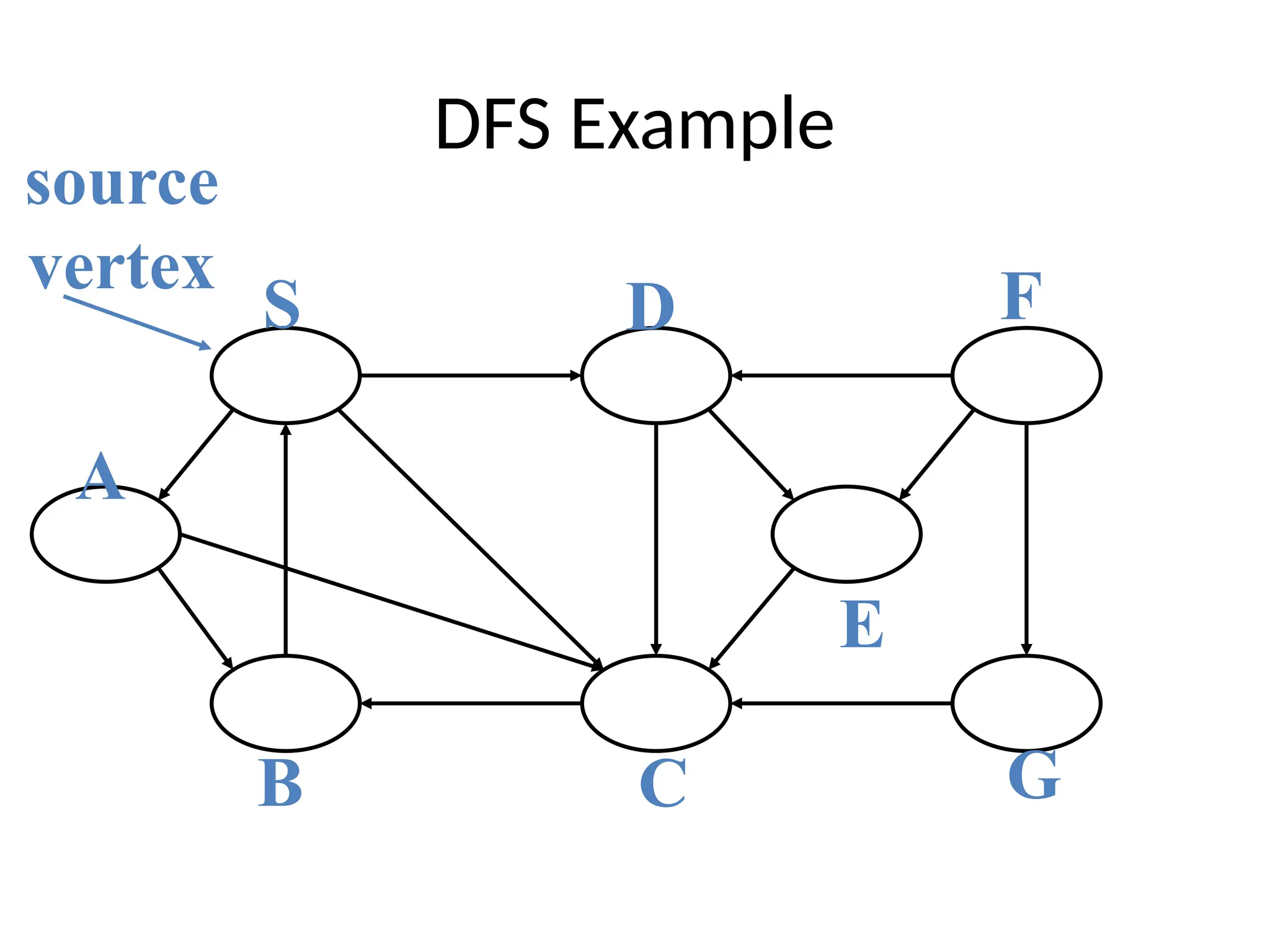
DFS Example
1 || |
|
|
|
| |
source
vertex
d f
S
A
B C
D
E
F
G
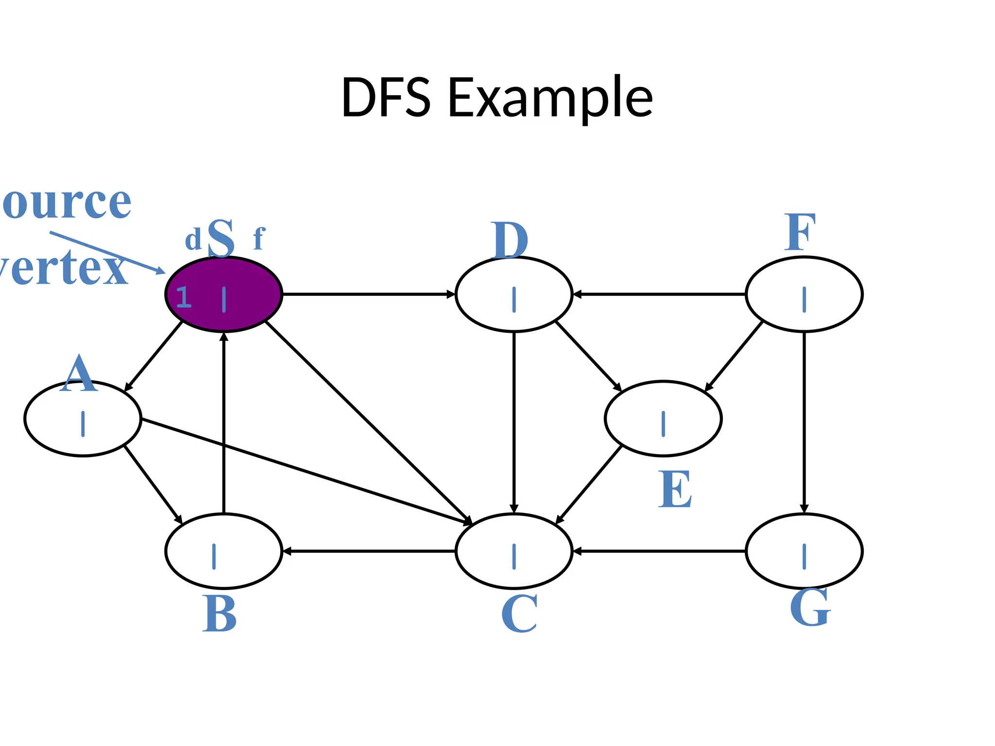
53.
DFS Example
1 || |
|
|
|
2 | |
source
vertex
d f
S
A
B C
D
E
F
G
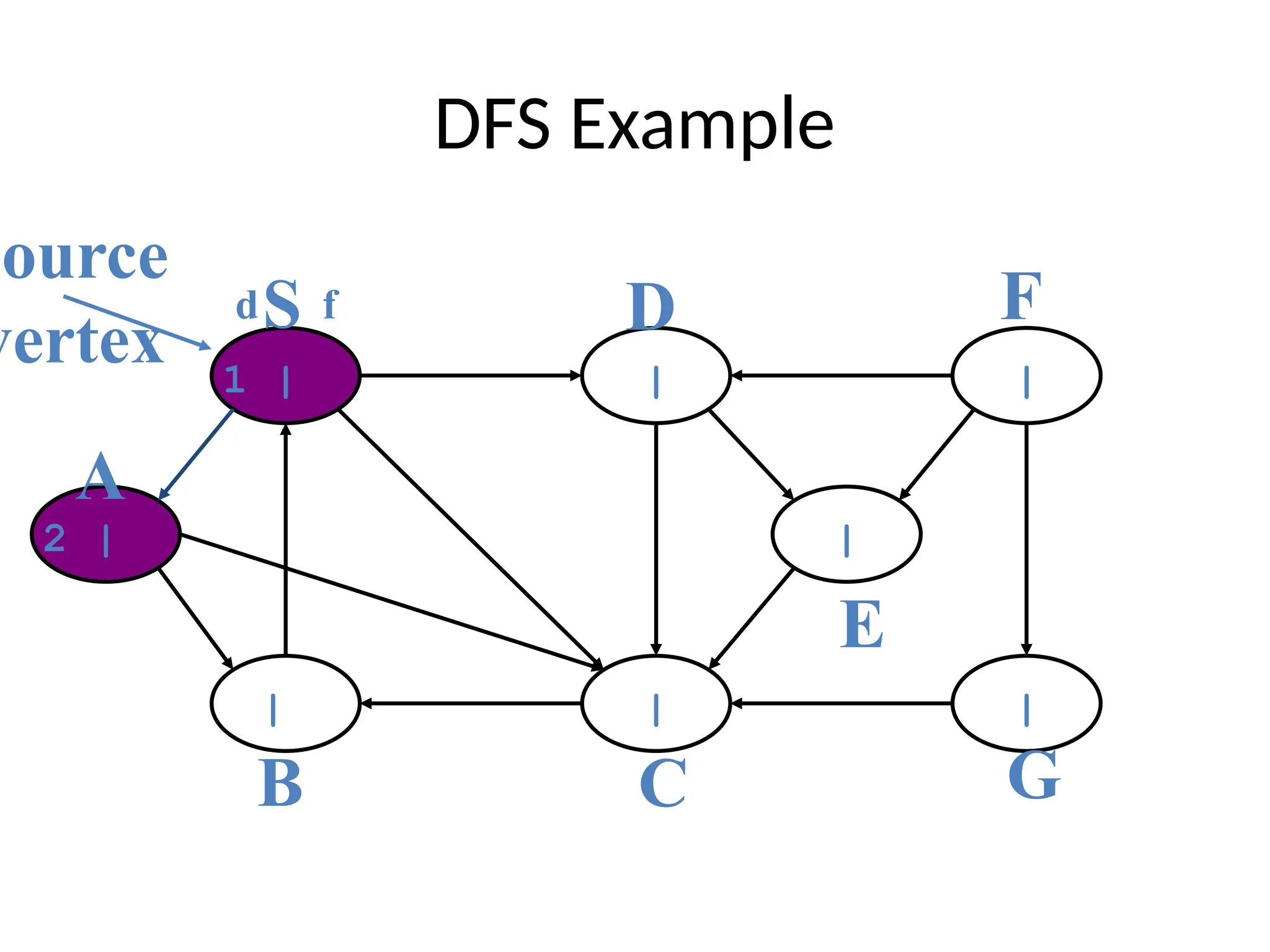
54.
DFS Example
1 || |
|
|
3 |
2 | |
source
vertex
d f
S
A
B C
D
E
F
G
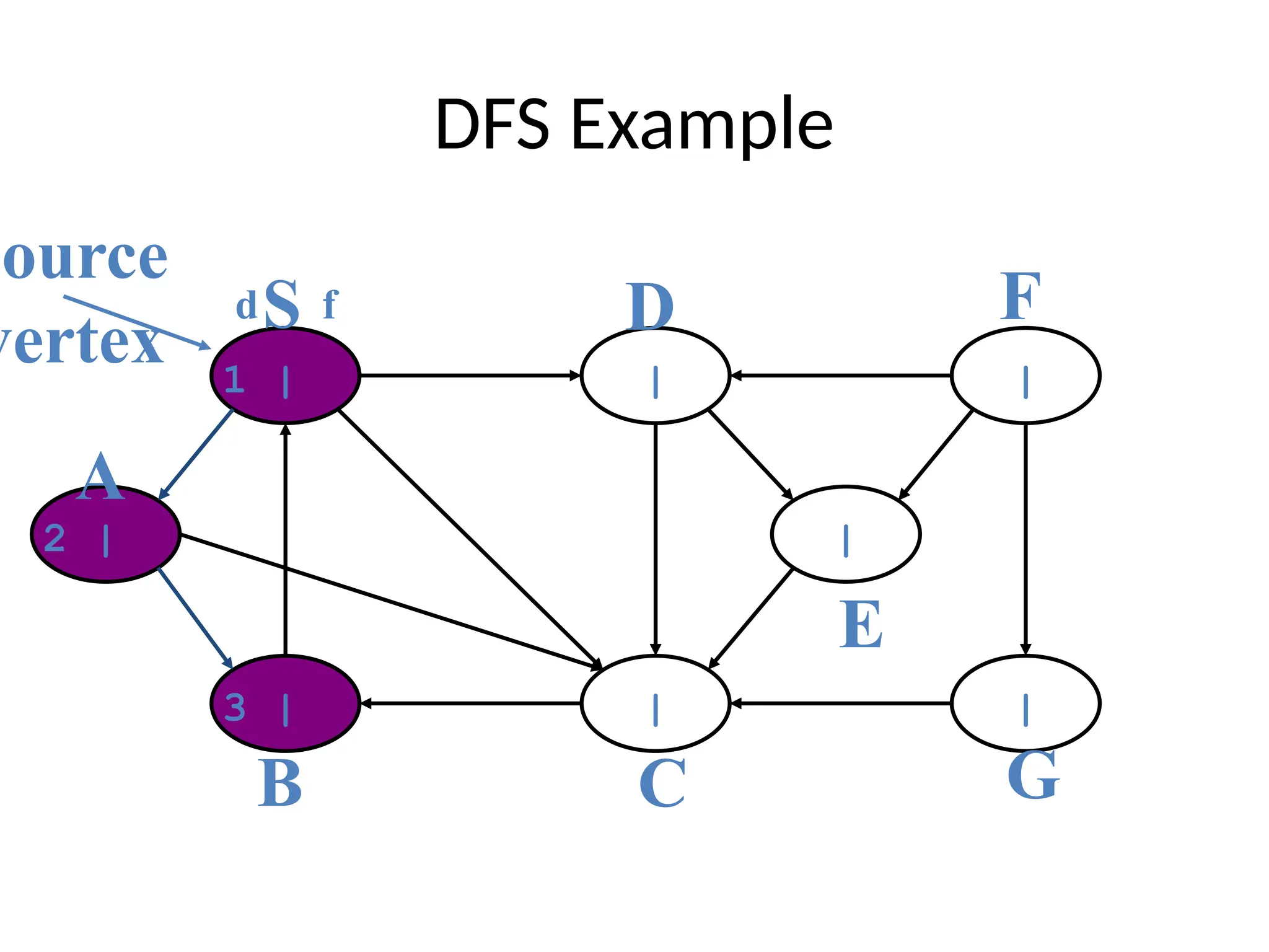
55.
DFS Example
1 || |
|
|
3 | 4
2 | |
source
vertex
d f
S
A
B C
D
E
F
G
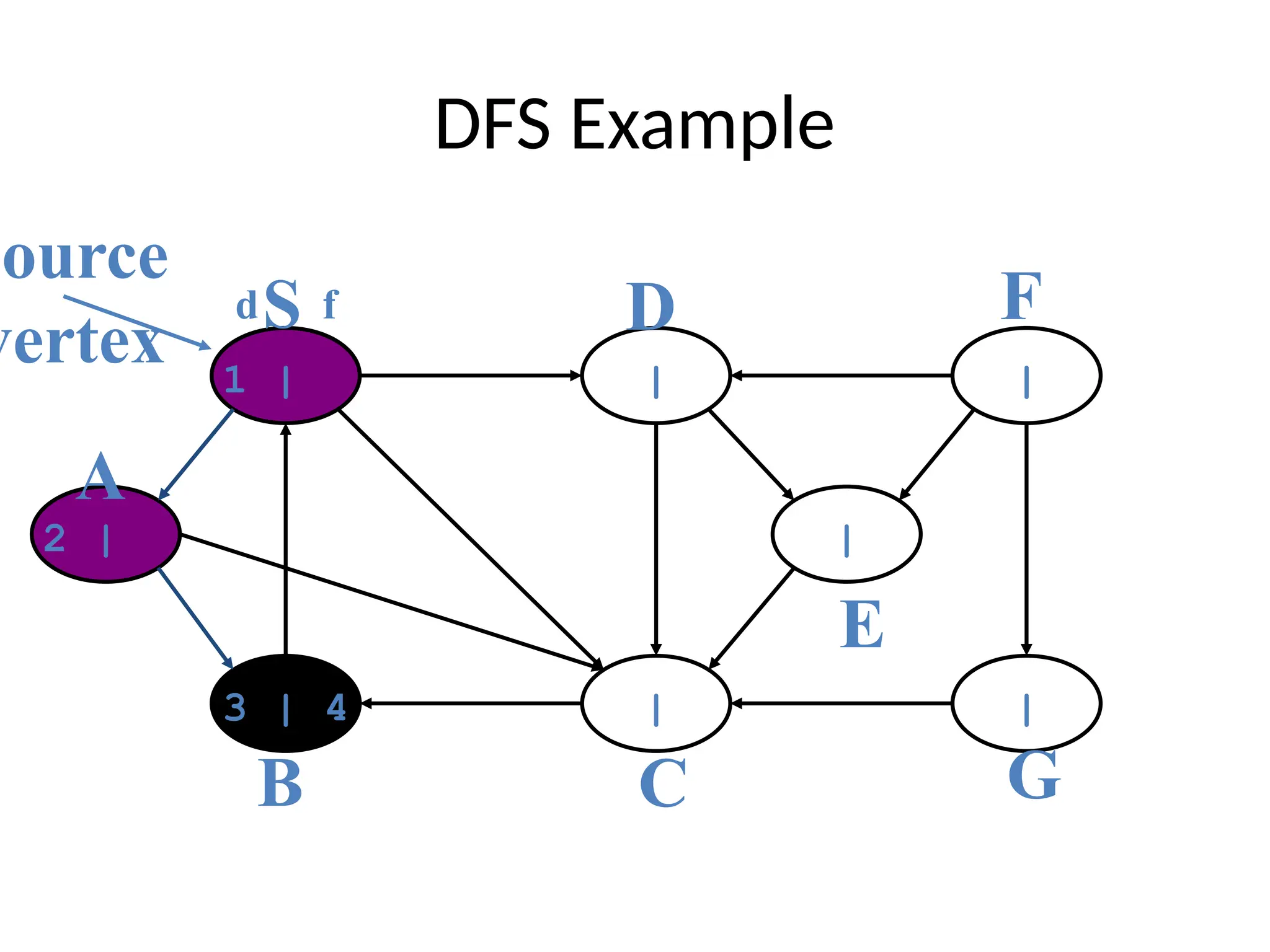
56.
DFS Example
1 || |
|
5 |
3 | 4
2 | |
source
vertex
d f
S
A
B C
D
E
F
G
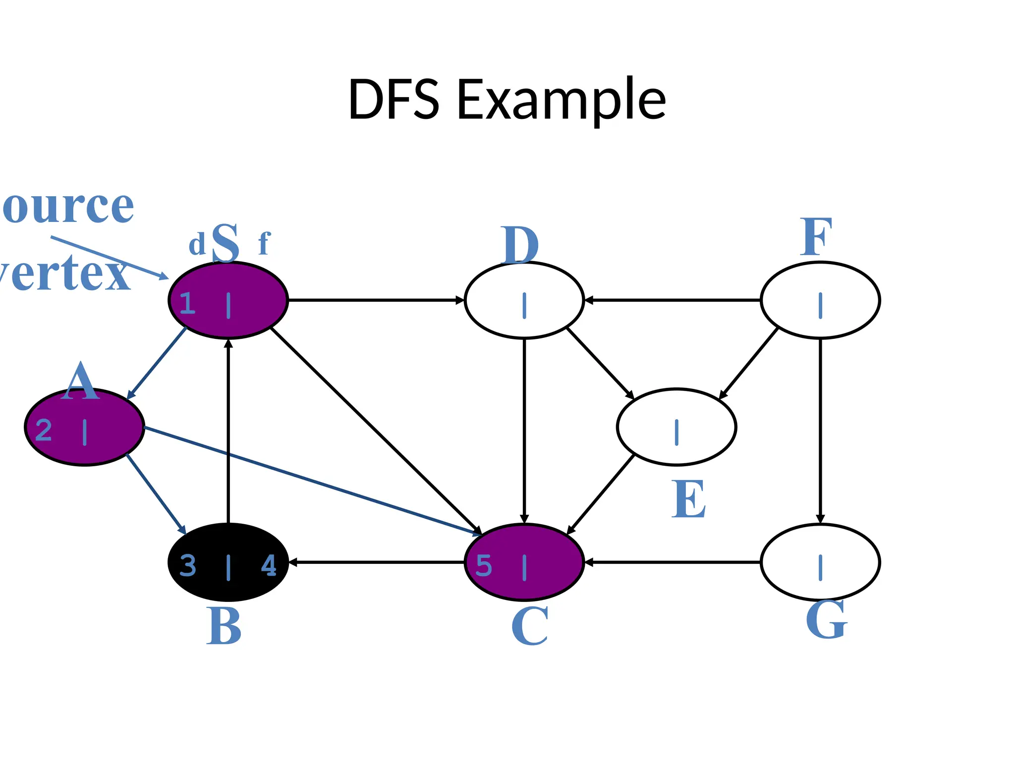
57.
DFS Example
1 || |
|
5 | 6
3 | 4
2 | |
source
vertex
d f
S
A
B C
D
E
F
G
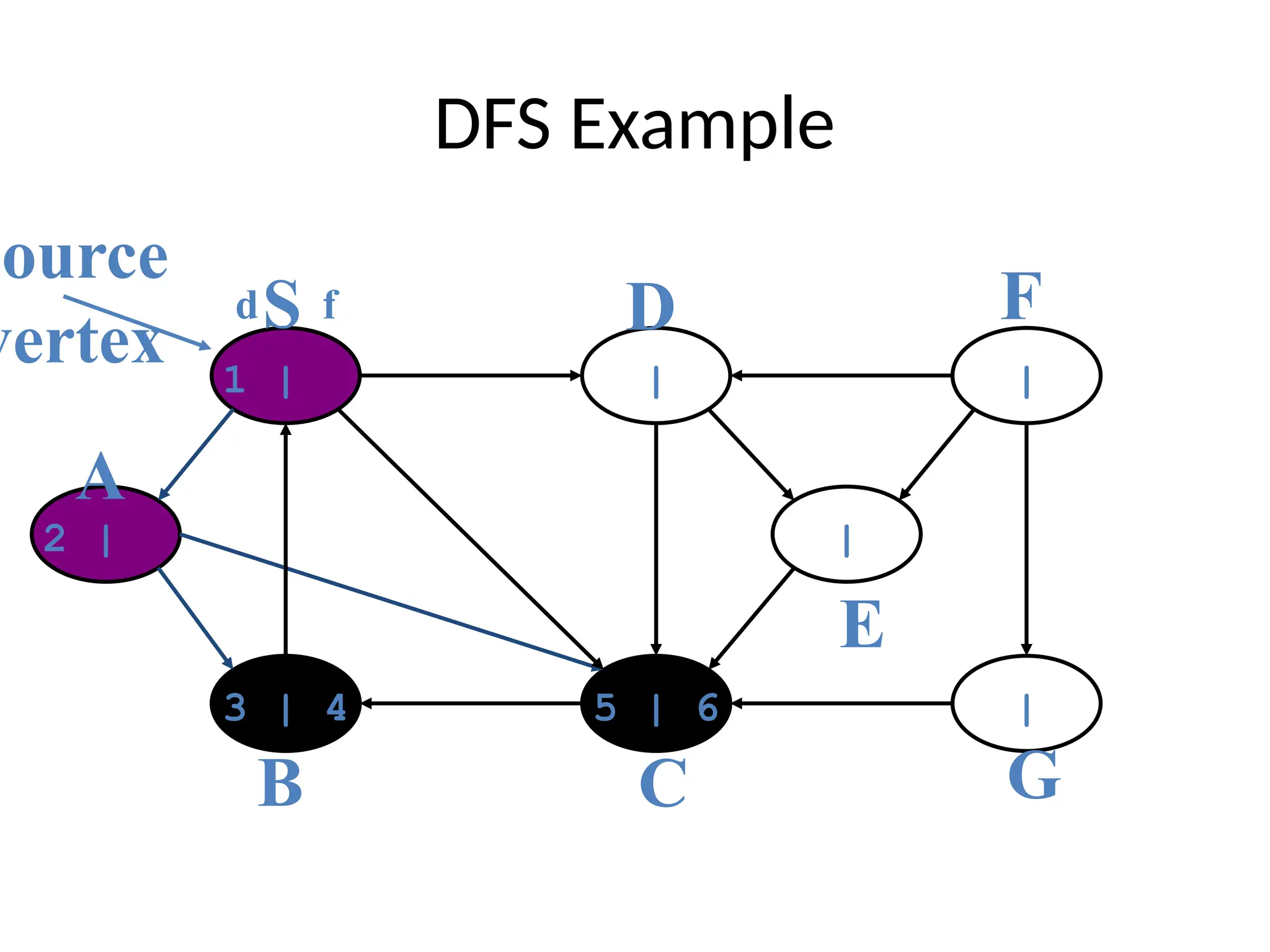
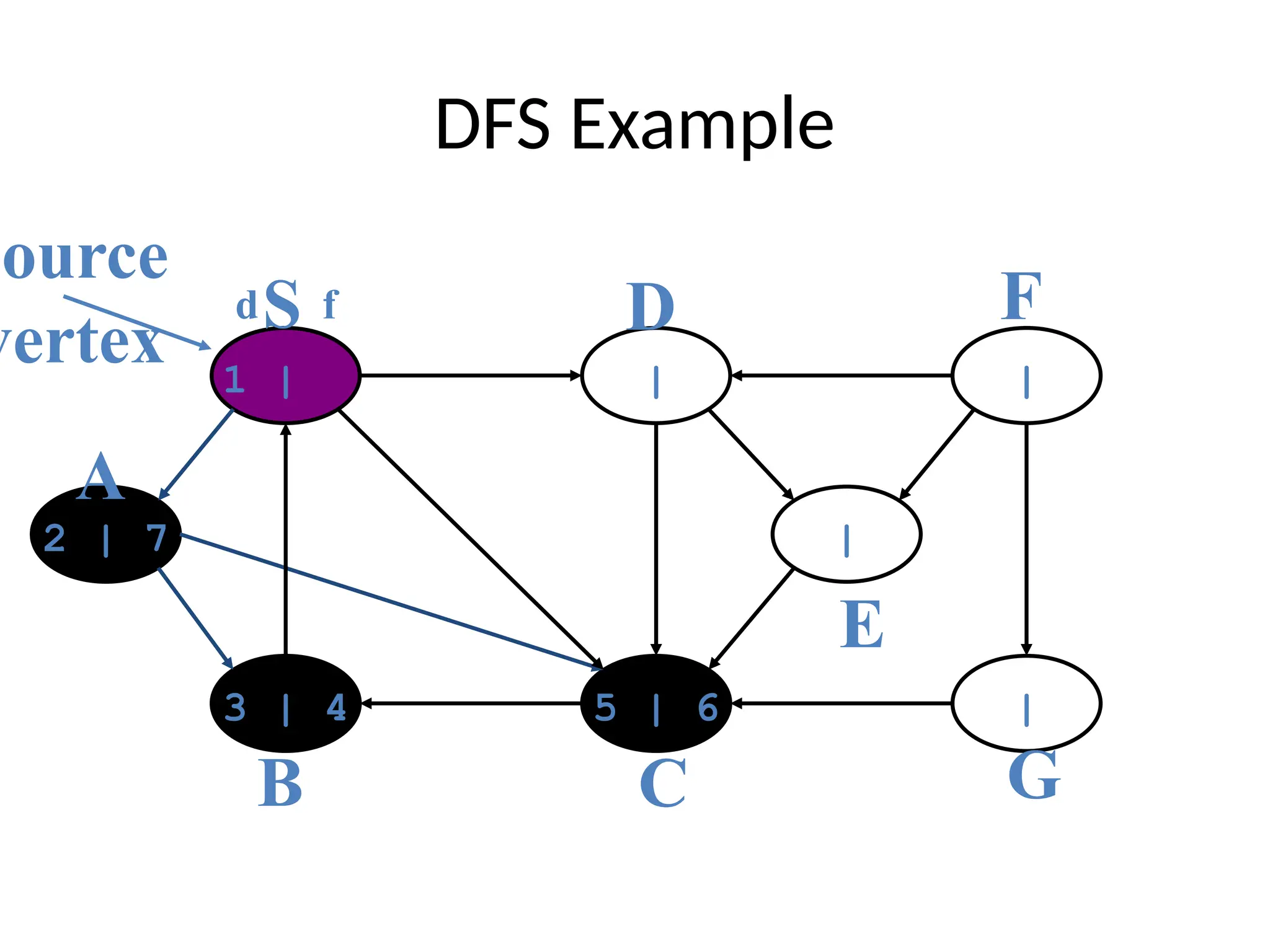
58.
DFS Example
1 || |
|
5 | 6
3 | 4
2 | 7 |
source
vertex
d f
S
A
B C
D
E
F
G
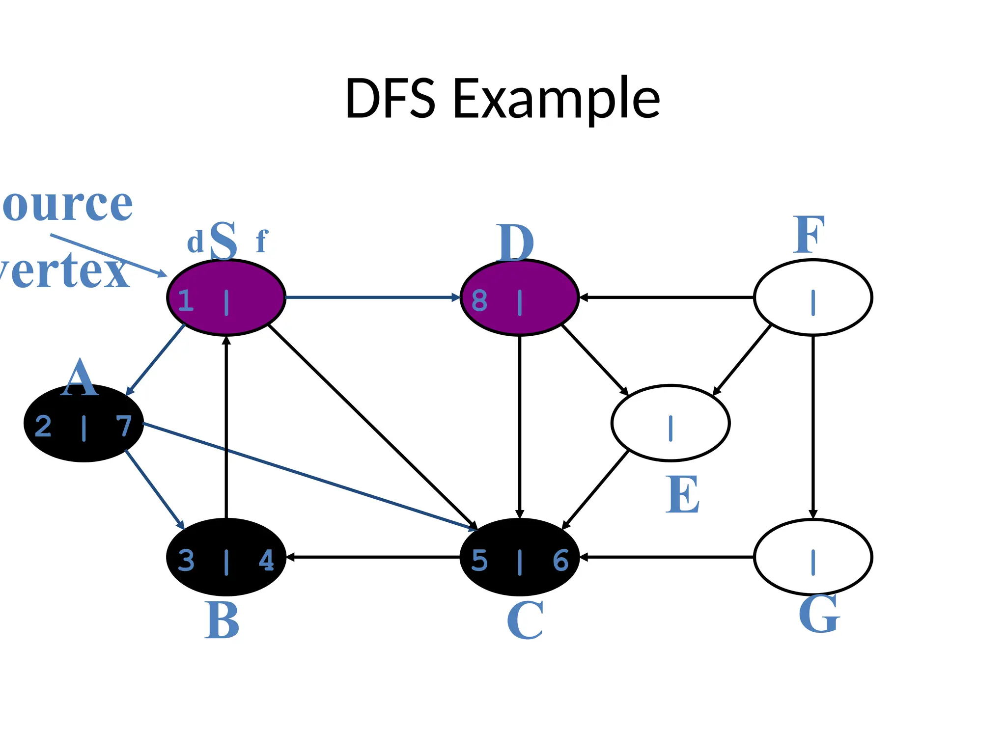
59.
DFS Example
1 |8 | |
|
5 | 6
3 | 4
2 | 7 |
source
vertex
d f
S
A
B C
D
E
F
G
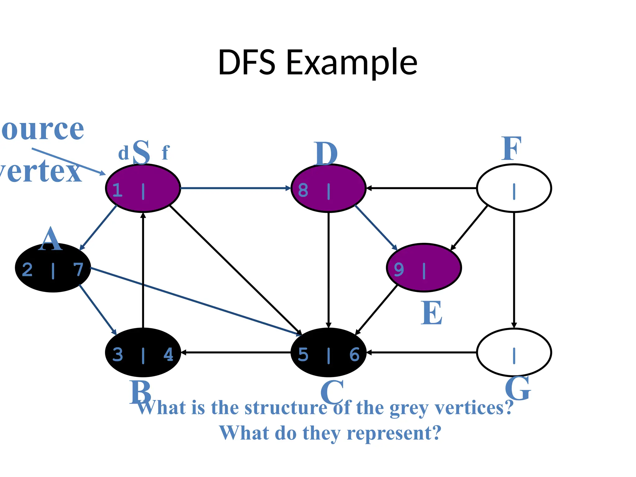
60.
DFS Example
1 |8 | |
|
5 | 6
3 | 4
2 | 7 9 |
source
vertex
d f
What is the structure of the grey vertices?
What do they represent?
S
A
B C
D
E
F
G
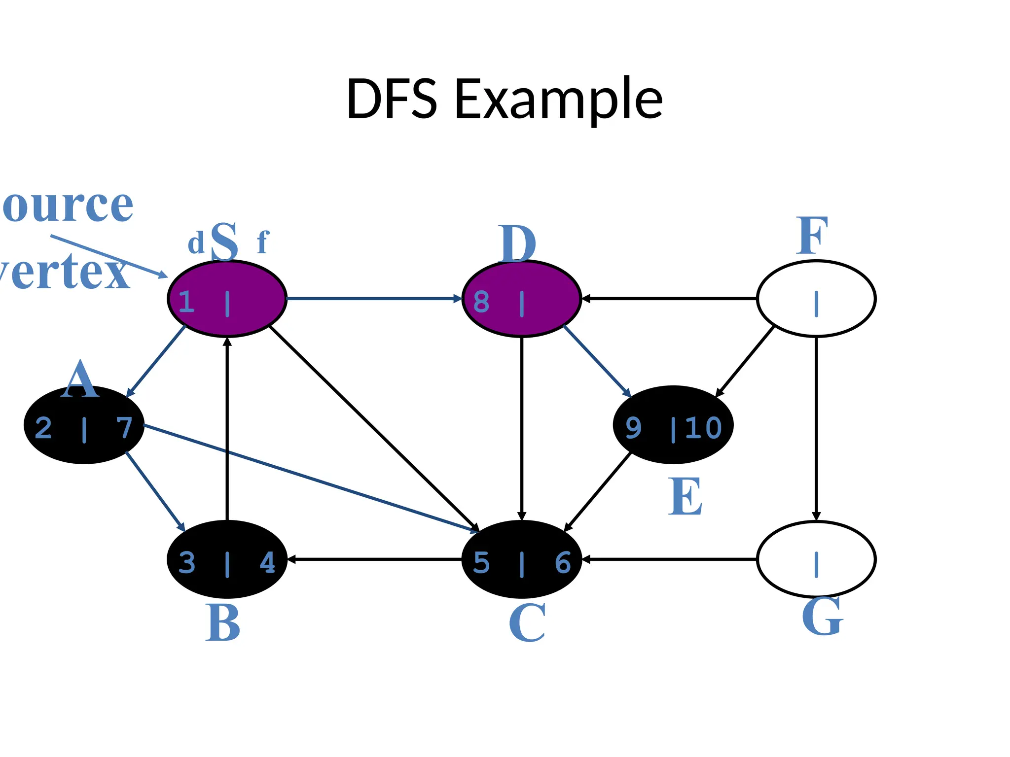
61.
DFS Example
1 |8 | |
|
5 | 6
3 | 4
2 | 7 9 |10
source
vertex
d f
S
A
B C
D
E
F
G
62.
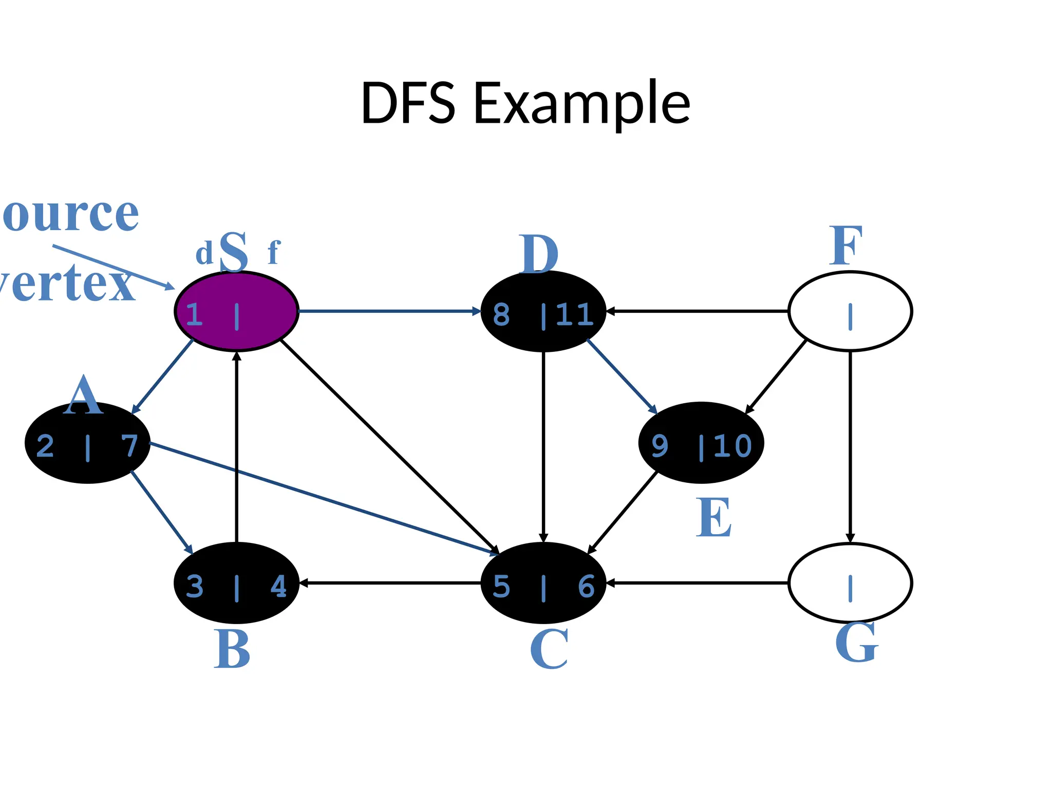
DFS Example
1 |8 |11 |
|
5 | 6
3 | 4
2 | 7 9 |10
source
vertex
d f
S
A
B C
D
E
F
G
63.
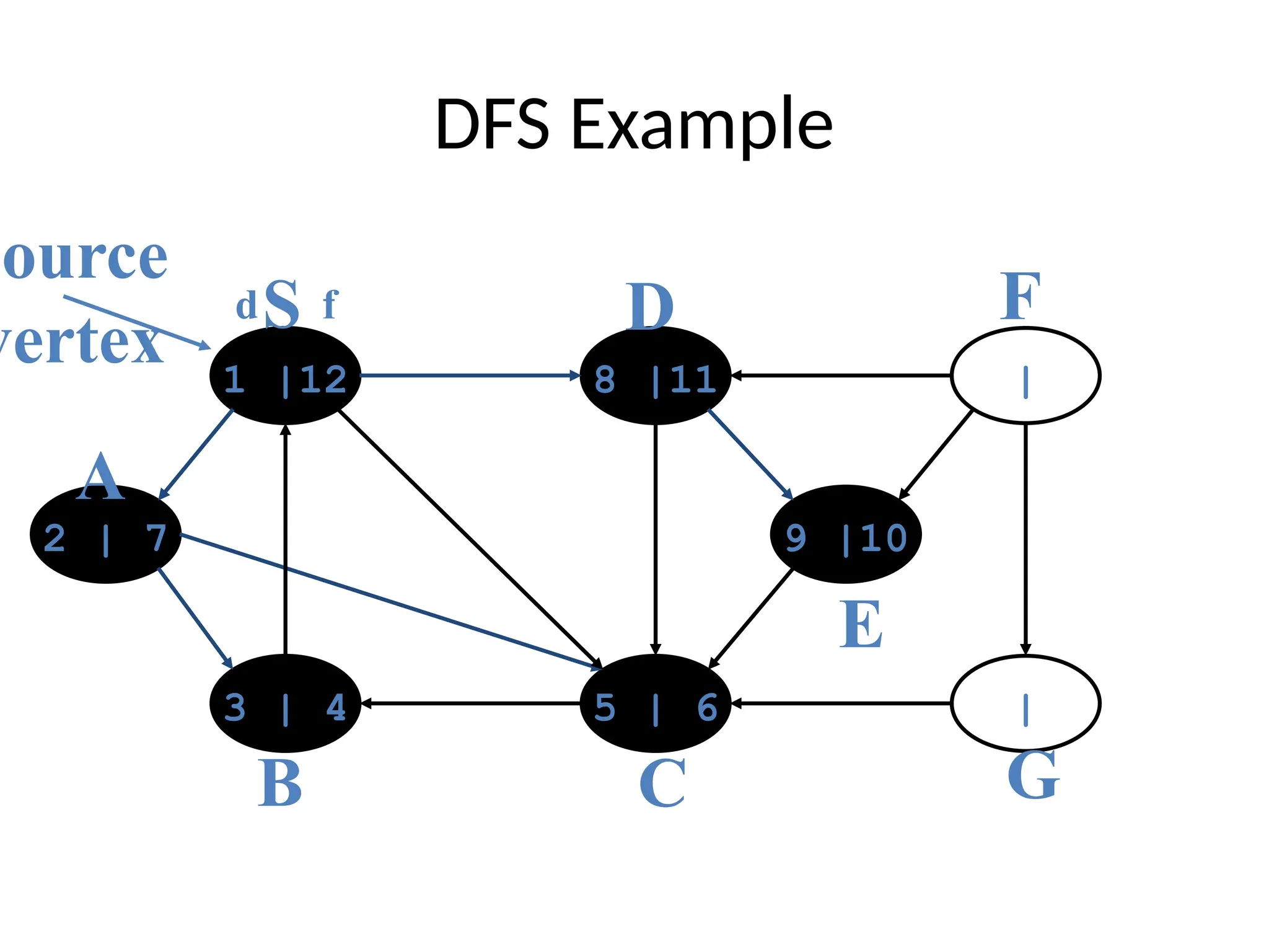
DFS Example
1 |128 |11 |
|
5 | 6
3 | 4
2 | 7 9 |10
source
vertex
d f
S
A
B C
D
E
F
G
64.
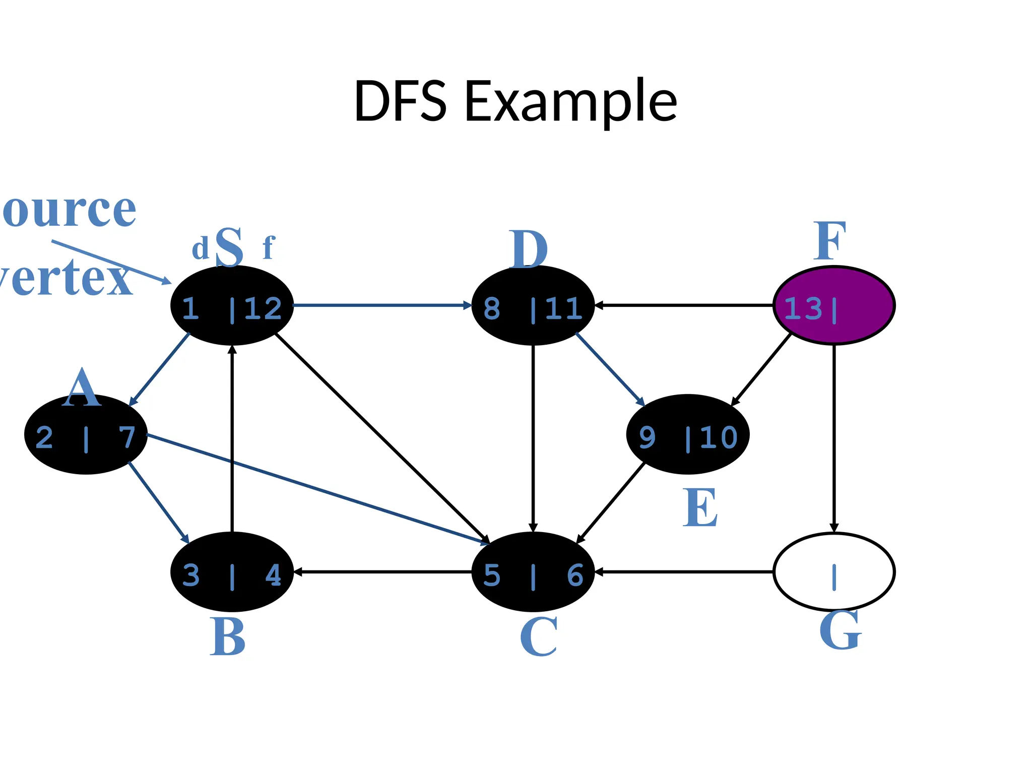
DFS Example
1 |128 |11 13|
|
5 | 6
3 | 4
2 | 7 9 |10
source
vertex
d f
S
A
B C
D
E
F
G
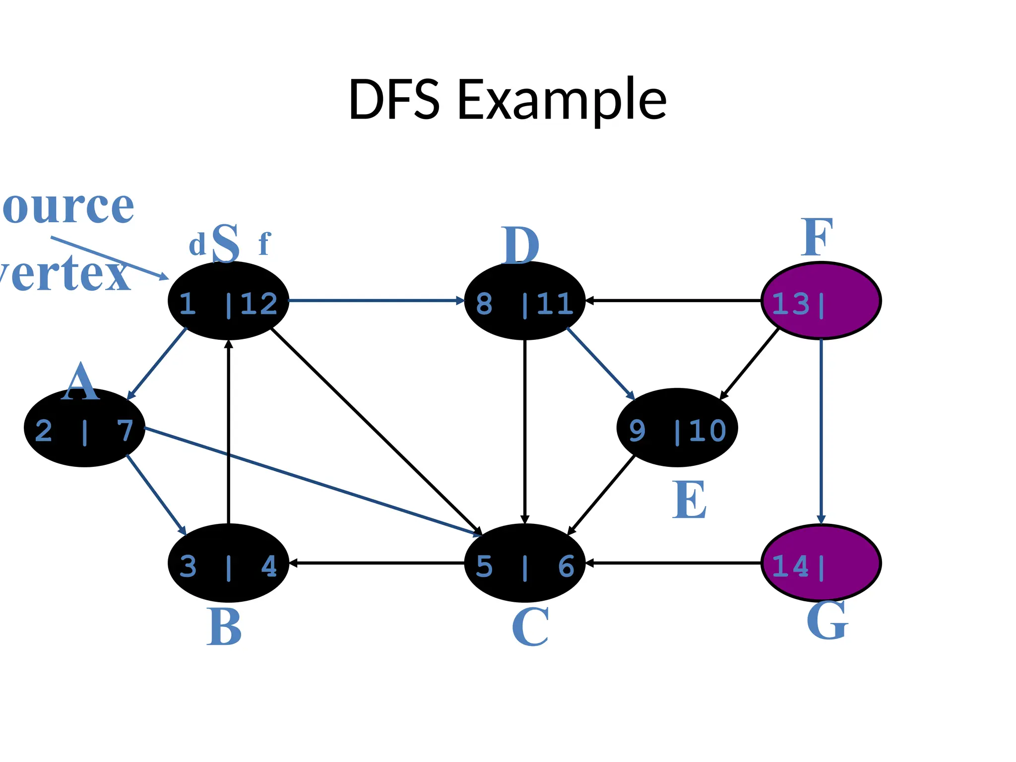
65.
DFS Example
1 |128 |11 13|
14|
5 | 6
3 | 4
2 | 7 9 |10
source
vertex
d f
S
A
B C
D
E
F
G
66.
DFS Example
1 |128 |11 13|
14|15
5 | 6
3 | 4
2 | 7 9 |10
source
vertex
d f
S
A
B C
D
E
F
G
67.
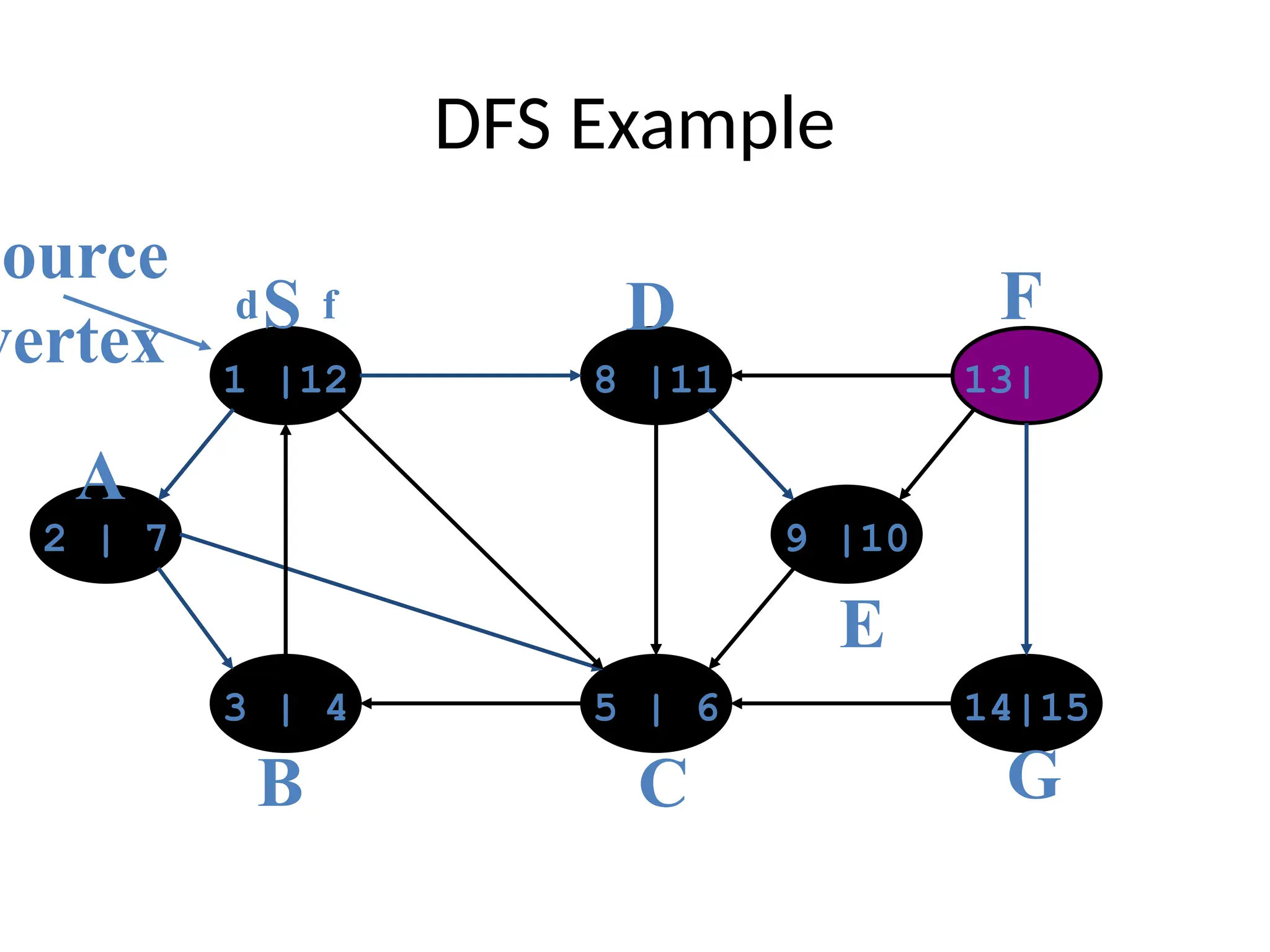
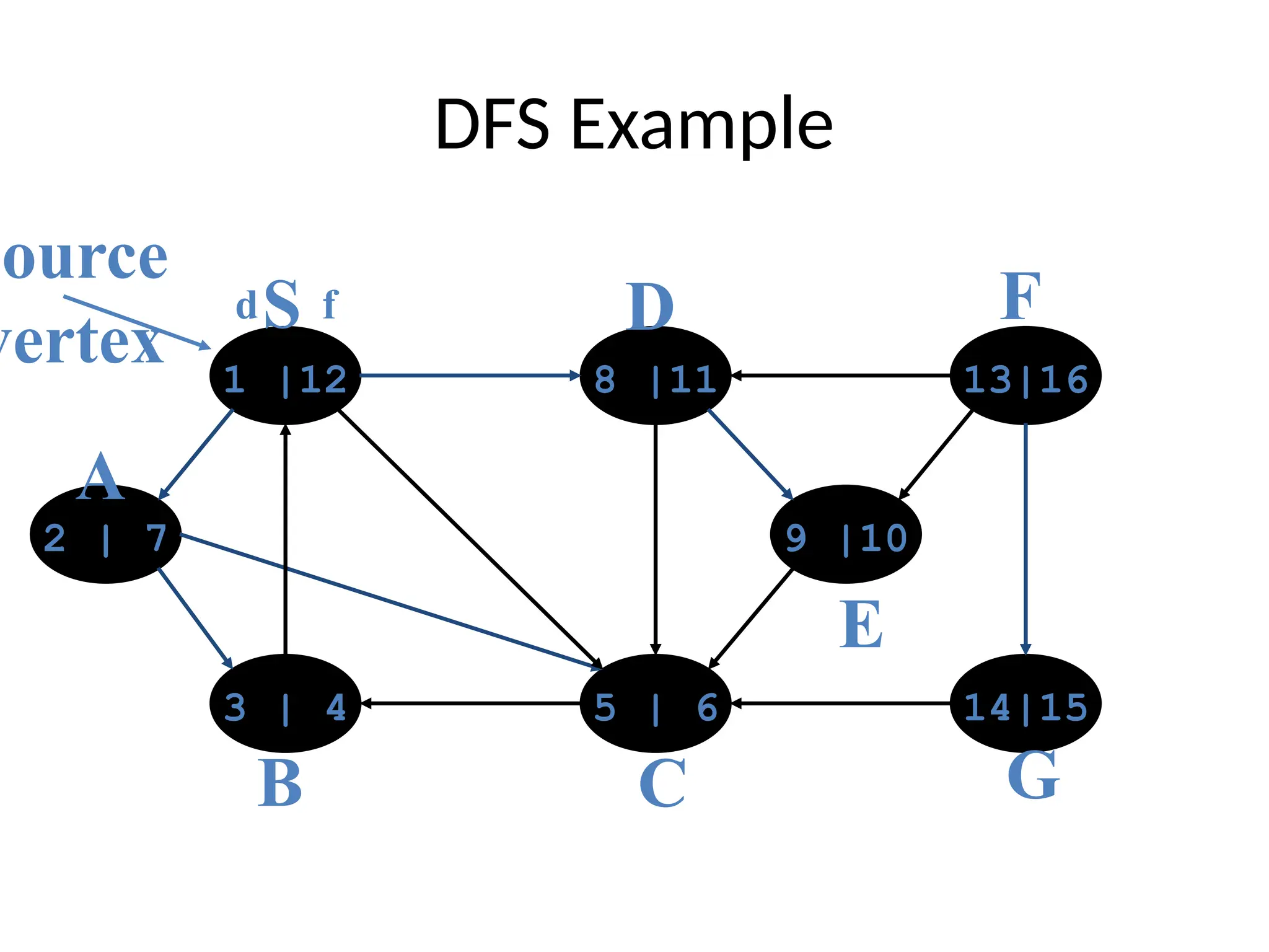
DFS Example
1 |128 |11 13|16
14|15
5 | 6
3 | 4
2 | 7 9 |10
source
vertex
d f
S
A
B C
D
E
F
G
68.
Depth-First Search: TheCode
Data: color[V], time,
prev[V],d[V], f[V]
DFS(G) // where prog starts
{
for each vertex u V
{
color[u] = WHITE;
prev[u]=NIL;
f[u]=inf;
d[u]=inf;
}
time = 0;
for each vertex u V
if (color[u] == WHITE)
DFS_Visit(u);
}
DFS_Visit(u)
{
color[u] = GREY;
time = time+1;
d[u] = time;
for each v Adj[u]
{
if (color[v] == WHITE)
prev[v]=u;
DFS_Visit(v);
}
color[u] = BLACK;
time = time+1;
f[u] = time;
}
What will be the running time?
69.
Depth-First Search: TheCode
Data: color[V], time,
prev[V],d[V], f[V]
DFS(G) // where prog starts
{
for each vertex u V
{
color[u] = WHITE;
prev[u]=NIL;
f[u]=inf;
d[u]=inf;
}
time = 0;
for each vertex u V
if (color[u] == WHITE)
DFS_Visit(u);
}
DFS_Visit(u)
{
color[u] = GREY;
time = time+1;
d[u] = time;
for each v Adj[u]
{
if (color[v] == WHITE)
prev[v]=u;
DFS_Visit(v);
}
color[u] = BLACK;
time = time+1;
f[u] = time;
}
Running time: O(V2
) because call DFS_Visit on each vertex,
and the loop over Adj[] can run as many as |V| times
O(V)
O(V)
O(V)
70.
Depth-First Search: TheCode
Data: color[V], time,
prev[V],d[V], f[V]
DFS(G) // where prog starts
{
for each vertex u V
{
color[u] = WHITE;
prev[u]=NIL;
f[u]=inf;
d[u]=inf;
}
time = 0;
for each vertex u V
if (color[u] == WHITE)
DFS_Visit(u);
}
DFS_Visit(u)
{
color[u] = GREY;
time = time+1;
d[u] = time;
for each v Adj[u]
{
if (color[v] == WHITE)
prev[v]=u;
DFS_Visit(v);
}
color[u] = BLACK;
time = time+1;
f[u] = time;
}
BUT, there is actually a tighter bound.
How many times will DFS_Visit() actually be called?
71.
Depth-First Search: TheCode
Data: color[V], time,
prev[V],d[V], f[V]
DFS(G) // where prog starts
{
for each vertex u V
{
color[u] = WHITE;
prev[u]=NIL;
f[u]=inf;
d[u]=inf;
}
time = 0;
for each vertex u V
if (color[u] == WHITE)
DFS_Visit(u);
}
DFS_Visit(u)
{
color[u] = GREY;
time = time+1;
d[u] = time;
for each v Adj[u]
{
if (color[v] == WHITE)
prev[v]=u;
DFS_Visit(v);
}
color[u] = BLACK;
time = time+1;
f[u] = time;
}
So, running time of DFS = O(V+E)
72.
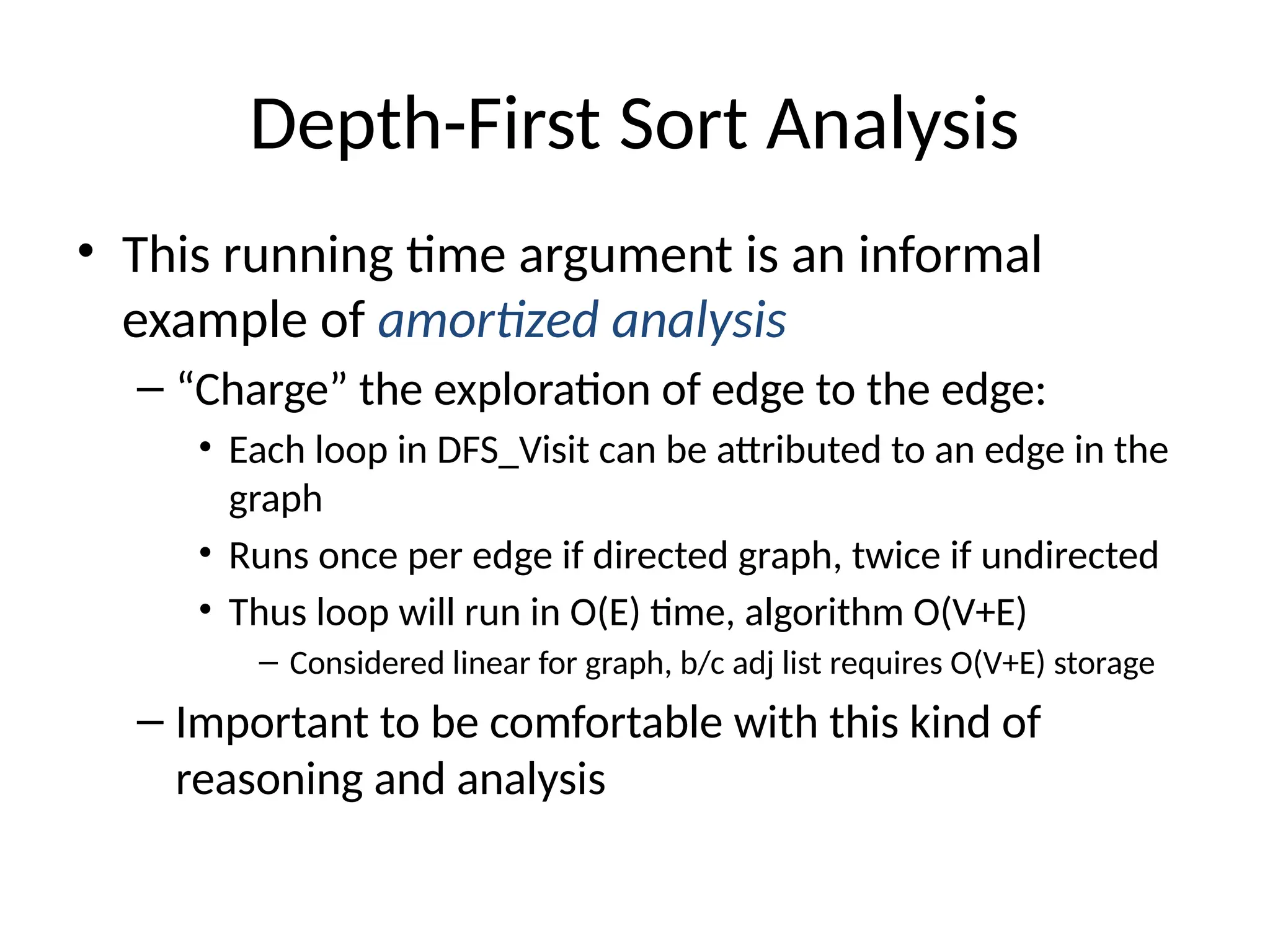
Depth-First Sort Analysis
•This running time argument is an informal
example of amortized analysis
– “Charge” the exploration of edge to the edge:
• Each loop in DFS_Visit can be attributed to an edge in the
graph
• Runs once per edge if directed graph, twice if undirected
• Thus loop will run in O(E) time, algorithm O(V+E)
– Considered linear for graph, b/c adj list requires O(V+E) storage
– Important to be comfortable with this kind of
reasoning and analysis
73.
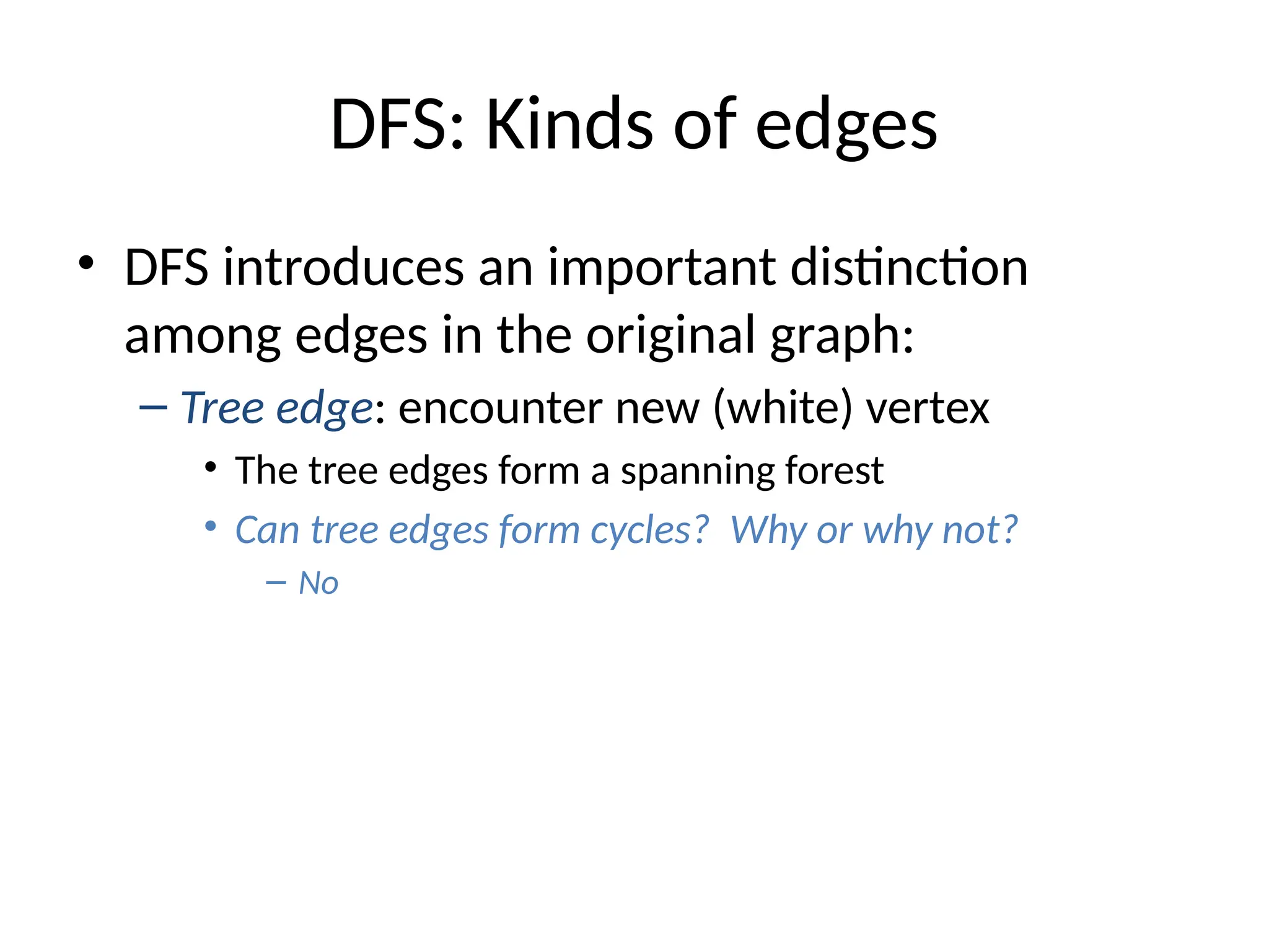
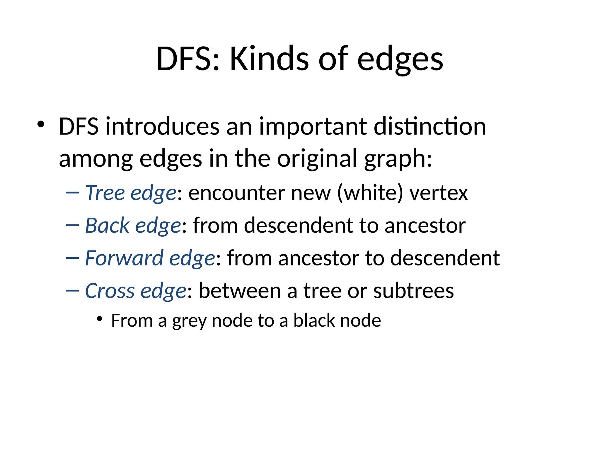
DFS: Kinds ofedges
• DFS introduces an important distinction
among edges in the original graph:
– Tree edge: encounter new (white) vertex
• The tree edges form a spanning forest
• Can tree edges form cycles? Why or why not?
– No
74.
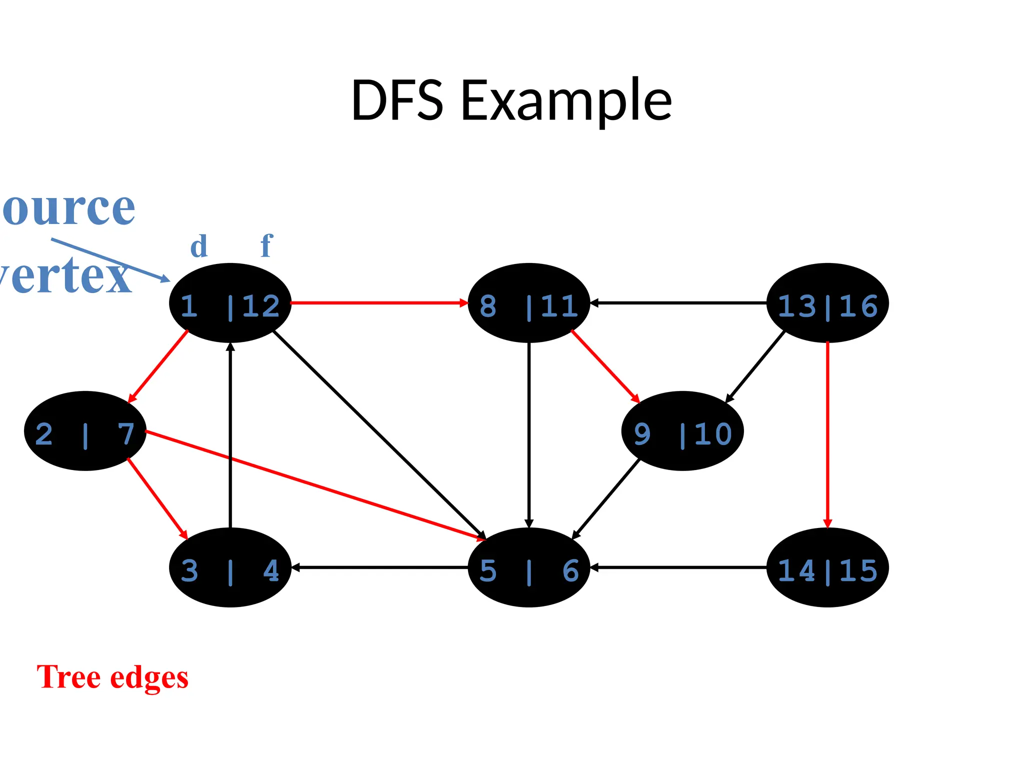
DFS Example
1 |128 |11 13|16
14|15
5 | 6
3 | 4
2 | 7 9 |10
source
vertex
d f
Tree edges
75.
DFS: Kinds ofedges
• DFS introduces an important distinction
among edges in the original graph:
– Tree edge: encounter new (white) vertex
– Back edge: from descendent to ancestor
• Encounter a grey vertex (grey to grey)
• Self loops are considered as to be back edge.
76.
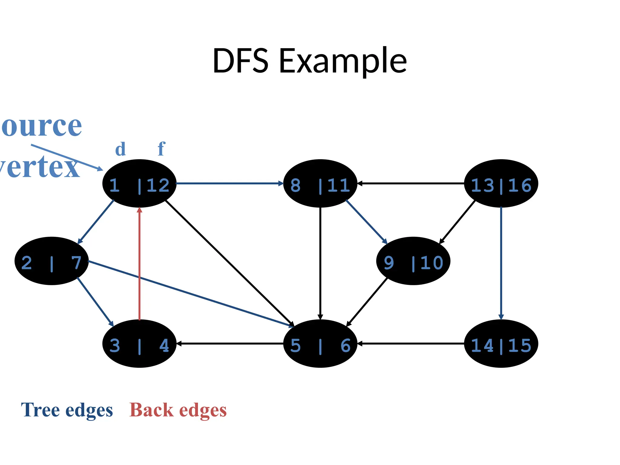
DFS Example
1 |128 |11 13|16
14|15
5 | 6
3 | 4
2 | 7 9 |10
source
vertex
d f
Tree edges Back edges
77.
DFS: Kinds ofedges
• DFS introduces an important distinction
among edges in the original graph:
– Tree edge: encounter new (white) vertex
– Back edge: from descendent to ancestor
– Forward edge: from ancestor to descendent
• Not a tree edge, though
• From grey node to black node
78.
DFS Example
1 |128 |11 13|16
14|15
5 | 6
3 | 4
2 | 7 9 |10
source
vertex
d f
Tree edges Back edges Forward edges
79.
DFS: Kinds ofedges
• DFS introduces an important distinction
among edges in the original graph:
– Tree edge: encounter new (white) vertex
– Back edge: from descendent to ancestor
– Forward edge: from ancestor to descendent
– Cross edge: between a tree or subtrees
• From a grey node to a black node
80.
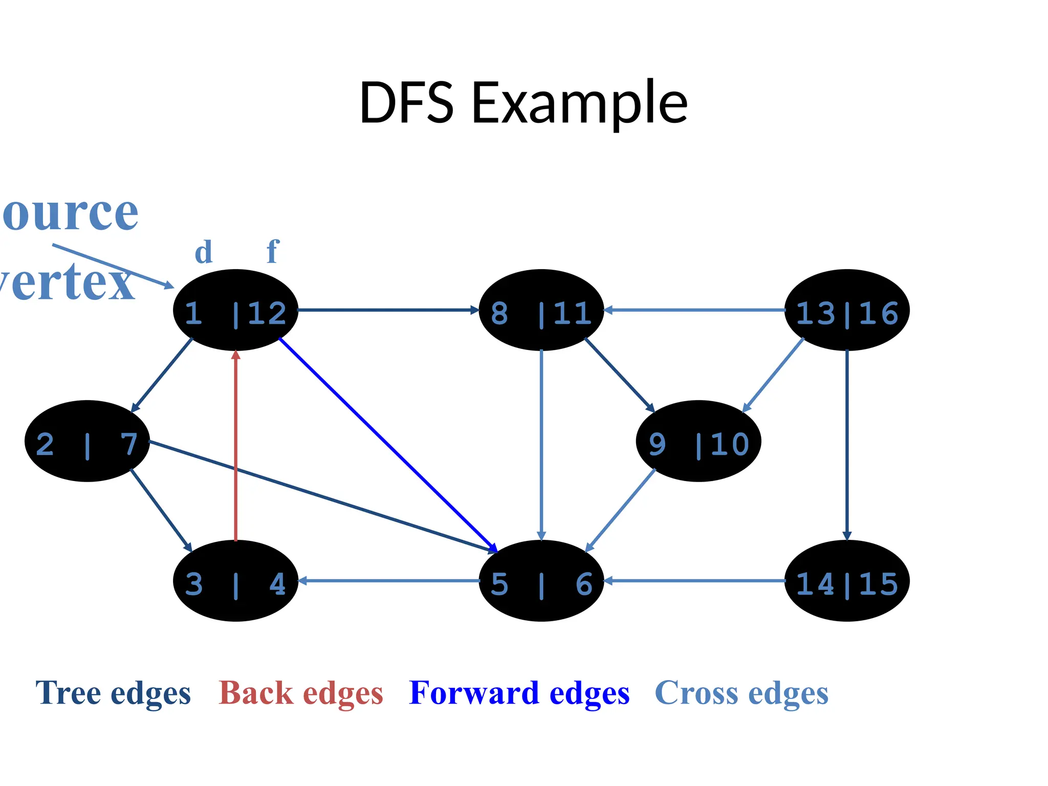
DFS Example
1 |128 |11 13|16
14|15
5 | 6
3 | 4
2 | 7 9 |10
source
vertex
d f
Tree edges Back edges Forward edges Cross edges
81.
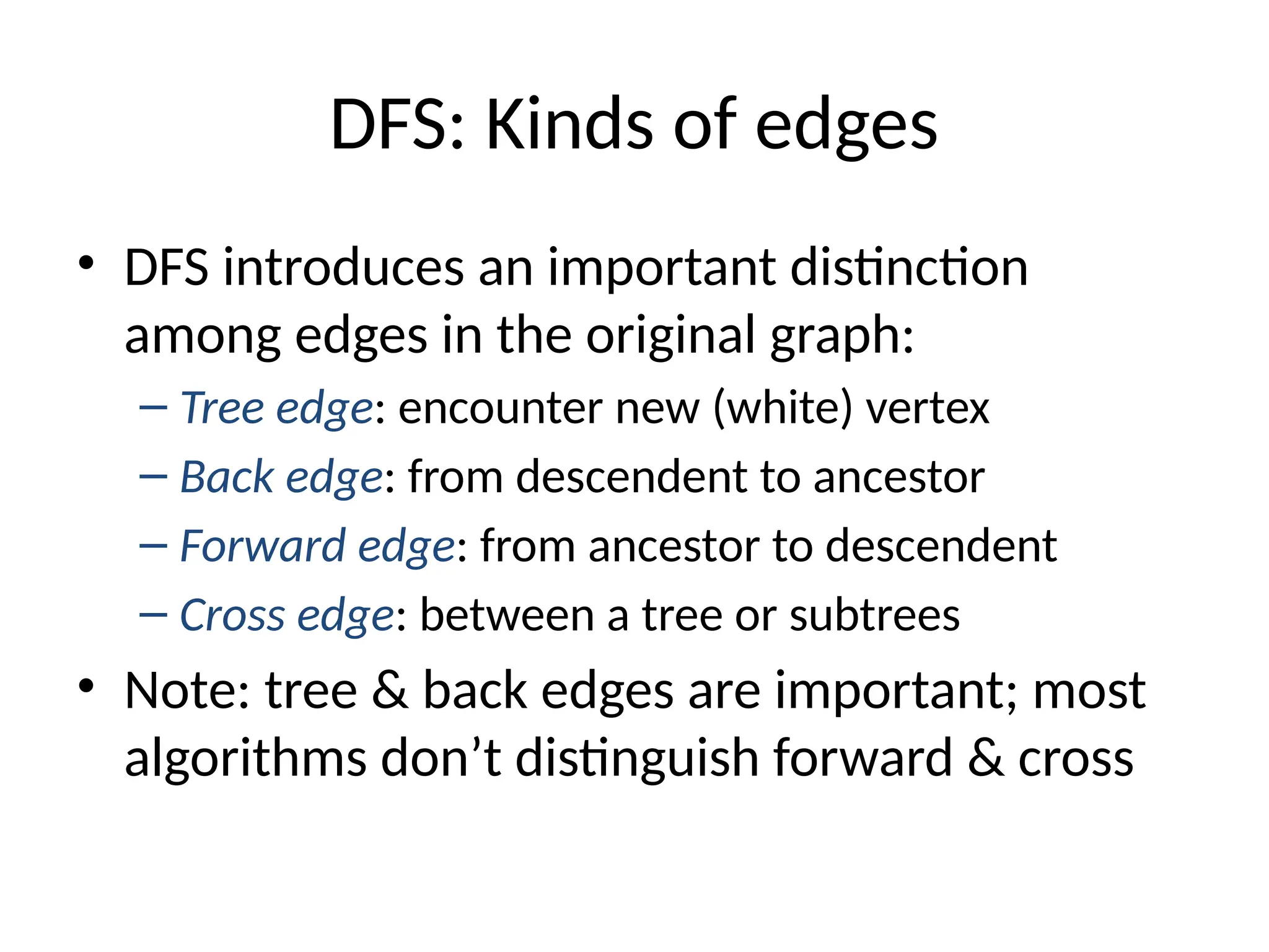
DFS: Kinds ofedges
• DFS introduces an important distinction
among edges in the original graph:
– Tree edge: encounter new (white) vertex
– Back edge: from descendent to ancestor
– Forward edge: from ancestor to descendent
– Cross edge: between a tree or subtrees
• Note: tree & back edges are important; most
algorithms don’t distinguish forward & cross
82.
More about theedges
• Let (u,v) is an edge.
– If (color[v] = WHITE) then (u,v) is a tree edge
– If (color[v] = GRAY) then (u,v) is a back edge
– If (color[v] = BLACK) then (u,v) is a forward/cross
edge
• Forward Edge: d[u]<d[v]
• Cross Edge: d[u]>d[v]
83.
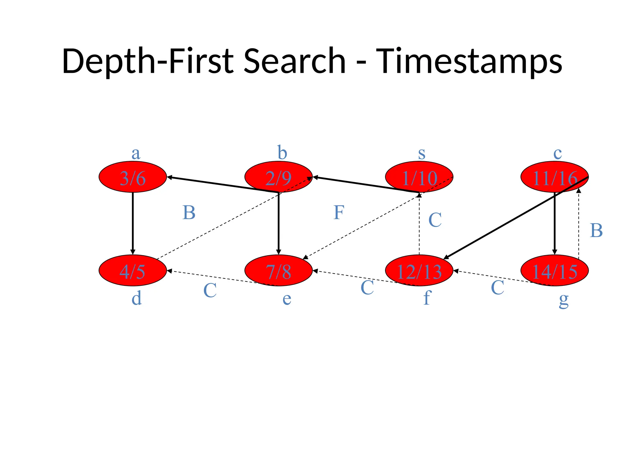
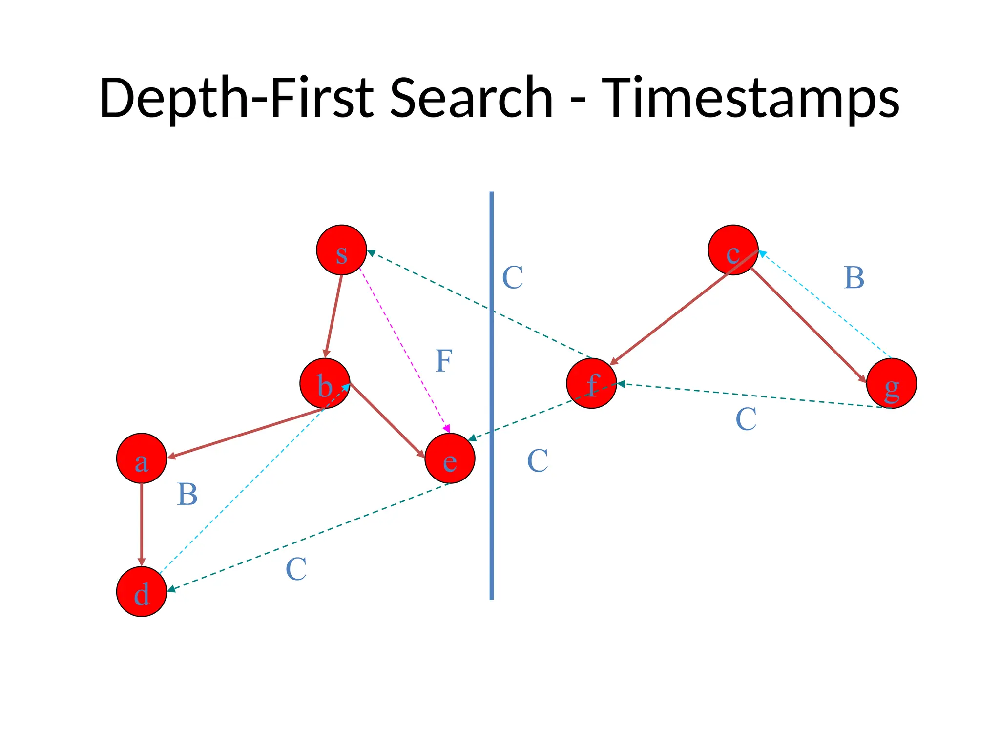
Depth-First Search -Timestamps
3/6
7/8
1/10
2/9
12/13
4/5
a b s
d e f
B F
11/16
14/15
c
g
C C
C
C
B
Depth-First Search: DetectEdge
Data: color[V], time,
prev[V],d[V], f[V]
DFS(G) // where prog starts
{
for each vertex u V
{
color[u] = WHITE;
prev[u]=NIL;
f[u]=inf;
d[u]=inf;
}
time = 0;
for each vertex u V
if (color[u] == WHITE)
DFS_Visit(u);
}
DFS_Visit(u)
{
color[u] = GREY;
time = time+1;
d[u] = time;
for each v Adj[u]
{
detect edge type using “color[v]”
if(color[v] == WHITE){
prev[v]=u;
DFS_Visit(v);
}}
color[u] = BLACK;
time = time+1;
f[u] = time;
}
86.
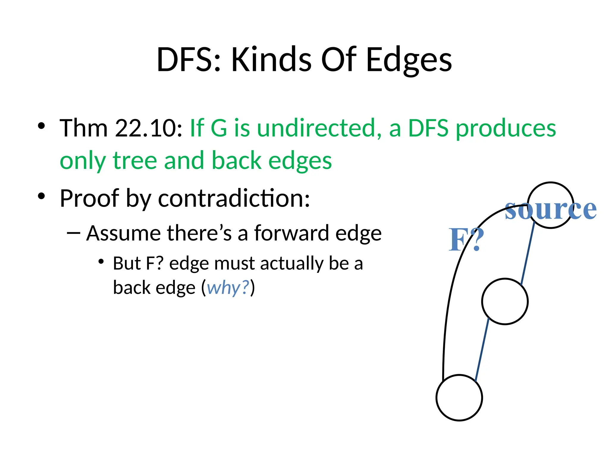
DFS: Kinds OfEdges
• Thm 22.10: If G is undirected, a DFS produces
only tree and back edges
• Proof by contradiction:
– Assume there’s a forward edge
• But F? edge must actually be a
back edge (why?)
source
F?
87.
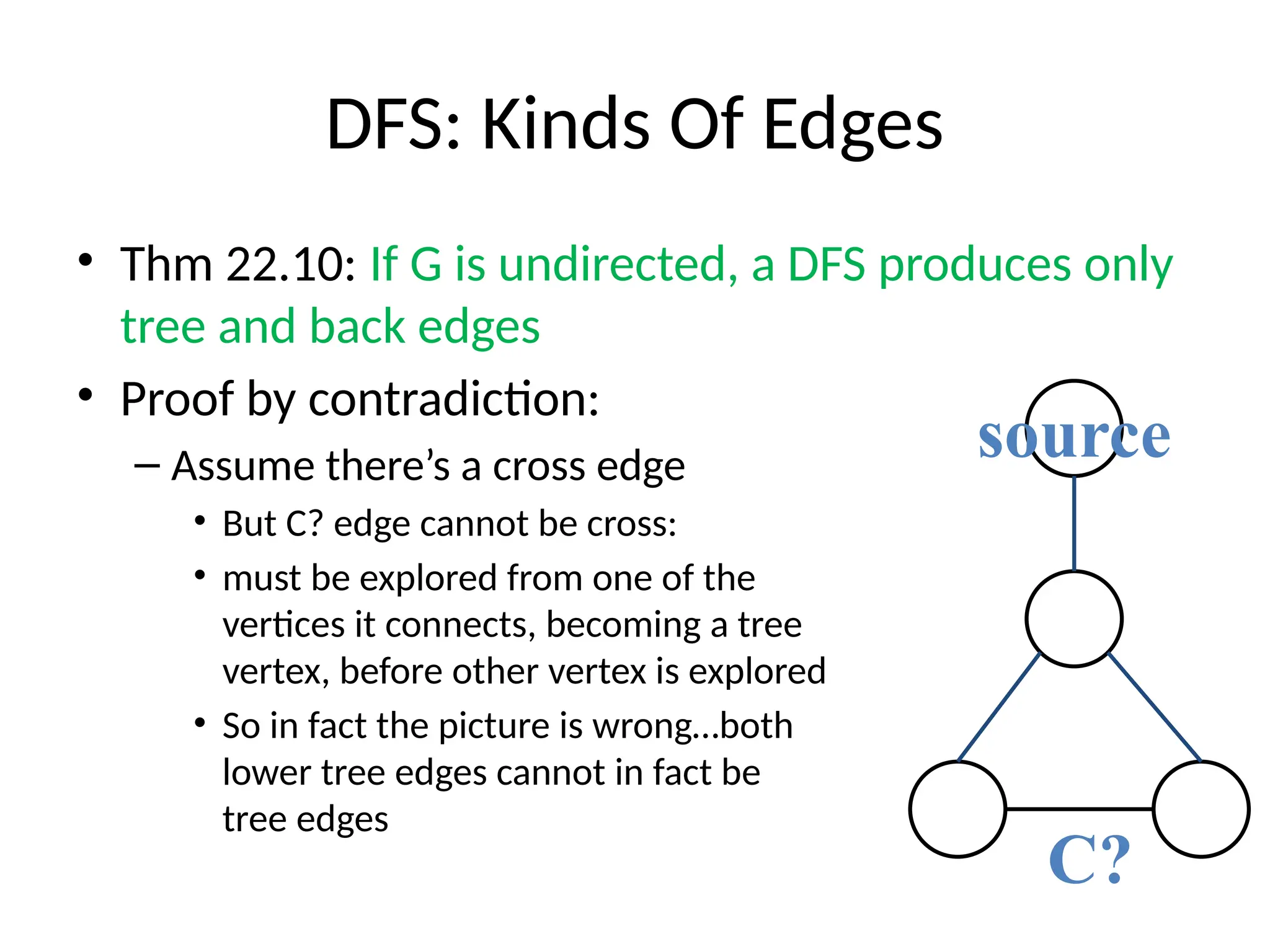
DFS: Kinds OfEdges
• Thm 22.10: If G is undirected, a DFS produces only
tree and back edges
• Proof by contradiction:
– Assume there’s a cross edge
• But C? edge cannot be cross:
• must be explored from one of the
vertices it connects, becoming a tree
vertex, before other vertex is explored
• So in fact the picture is wrong…both
lower tree edges cannot in fact be
tree edges
source
C?
88.
DFS And GraphCycles
• Thm: An undirected graph is acyclic iff a DFS yields
no back edges
– If acyclic, no back edges (because a back edge implies a
cycle
– If no back edges, acyclic
• No back edges implies only tree edges (Why?)
• Only tree edges implies we have a tree or a forest
• Which by definition is acyclic
• Thus, can run DFS to find whether a graph has a
cycle
89.
DFS And Cycles
Data:color[V], time,
prev[V],d[V], f[V]
DFS(G) // where prog starts
{
for each vertex u V
{
color[u] = WHITE;
prev[u]=NIL;
f[u]=inf; d[u]=inf;
}
time = 0;
for each vertex u V
if (color[u] == WHITE)
DFS_Visit(u);
}
DFS_Visit(u)
{
color[u] = GREY;
time = time+1;
d[u] = time;
for each v Adj[u]
{
if (color[v]==WHITE){
prev[v]=u;
DFS_Visit(v);
}
}
color[u] = BLACK;
time = time+1;
f[u] = time;
}
How would you modify the code to detect
cycles?
90.
DFS And Cycles
Data:color[V], time,
prev[V],d[V], f[V]
DFS(G) // where prog starts
{
for each vertex u V
{
color[u] = WHITE;
prev[u]=NIL;
f[u]=inf; d[u]=inf;
}
time = 0;
for each vertex u V
if (color[u] == WHITE)
DFS_Visit(u);
}
DFS_Visit(u)
{
color[u] = GREY;
time = time+1;
d[u] = time;
for each v Adj[u]
{
if (color[v]==WHITE){
prev[v]=u;
DFS_Visit(v); }
else {cycle exists;}
}
color[u] = BLACK;
time = time+1;
f[u] = time;
}
What will be the running time?
91.
DFS And Cycles
•What will be the running time for undirected
graph to detect cycle?
• A: O(V+E)
• We can actually determine if cycles exist in
O(V) time
– How??
92.
DFS And Cycles
•What will be the running time for undirected
graph to detect cycle?
• A: O(V+E)
• We can actually determine if cycles exist in
O(V) time:
– In an undirected acyclic forest, |E| |V| - 1
– So count the edges: if ever see |V| distinct edges,
must have seen a back edge along the way
93.
DFS And Cycles
•What will be the running time for directed
graph to detect cycle?
• A: O(V+E)
Some applications ofBFS and DFS
• Topological Sort (Topic of Next Lecture)
• Euler Path (Topic of Next Lecture)
• Dictionary Search
• Mathematical Problem
• Grid Traversal
96.
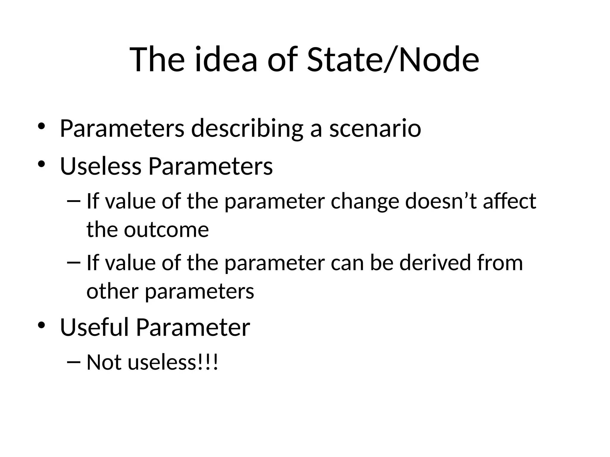
The idea ofState/Node
• Parameters describing a scenario
• Useless Parameters
– If value of the parameter change doesn’t affect
the outcome
– If value of the parameter can be derived from
other parameters
• Useful Parameter
– Not useless!!!
97.
Example - States
•Grid Problem, direction change takes time
• Grid Problem, blocks alternating


![Definition
• Path: the sequence of vertices to go through from one vertex to
another.
– a path from A to C is [A, B, C], or [A, G, B, C], or [A, E, F, D, B, C].
• Path Length: the number of edges in a path.
• Cycle: a path where the starting point and endpoint are the same
vertex.
– [A, B, D, F, E] forms a cycle. Similarly, [A, G, B] forms another cycle.](https://image.slidesharecdn.com/lecture1bfsdfs-250224160747-a8f05ee1/75/Design-and-analysis-of-Algorithms-Lecture-1-BFS-DFS-ppsx-10-2048.jpg)
![Breadth-First Search: The Code
Data: color[V], prev[V],d[V]
BFS(G) // starts from here
{
for each vertex u V-
{s}
{
color[u]=WHITE;
prev[u]=NIL;
d[u]=inf;
}
color[s]=GRAY;
d[s]=0; prev[s]=NIL;
Q=empty;
ENQUEUE(Q,s);
While(Q not empty)
{
u = DEQUEUE(Q);
for each v adj[u]{
if (color[v] == WHITE){
color[v] = GREY;
d[v] = d[u] + 1;
prev[v] = u;
Enqueue(Q, v);
}
}
color[u] = BLACK;
}
}](https://image.slidesharecdn.com/lecture1bfsdfs-250224160747-a8f05ee1/75/Design-and-analysis-of-Algorithms-Lecture-1-BFS-DFS-ppsx-27-2048.jpg)
![BFS: The Code (again)
Data: color[V], prev[V],d[V]
BFS(G) // starts from here
{
for each vertex u V-
{s}
{
color[u]=WHITE;
prev[u]=NIL;
d[u]=inf;
}
color[s]=GRAY;
d[s]=0; prev[s]=NIL;
Q=empty;
ENQUEUE(Q,s);
While(Q not empty)
{
u = DEQUEUE(Q);
for each v adj[u]{
if (color[v] == WHITE){
color[v] = GREY;
d[v] = d[u] + 1;
prev[v] = u;
Enqueue(Q, v);
}
}
color[u] = BLACK;
}
}](https://image.slidesharecdn.com/lecture1bfsdfs-250224160747-a8f05ee1/75/Design-and-analysis-of-Algorithms-Lecture-1-BFS-DFS-ppsx-38-2048.jpg)
![Breadth-First Search: Print Path
Data: color[V], prev[V],d[V]
Print-Path(G, s, v)
{
if(v==s)
print(s)
else if(prev[v]==NIL)
print(No path);
else{
Print-Path(G,s,prev[v]);
print(v);
}
}](https://image.slidesharecdn.com/lecture1bfsdfs-250224160747-a8f05ee1/75/Design-and-analysis-of-Algorithms-Lecture-1-BFS-DFS-ppsx-39-2048.jpg)
![BFS: Complexity
Data: color[V], prev[V],d[V]
BFS(G) // starts from here
{
for each vertex u V-
{s}
{
color[u]=WHITE;
prev[u]=NIL;
d[u]=inf;
}
color[s]=GRAY;
d[s]=0; prev[s]=NIL;
Q=empty;
ENQUEUE(Q,s);
While(Q not empty)
{
u = DEQUEUE(Q);
for each v adj[u]{
if(color[v] == WHITE){
color[v] = GREY;
d[v] = d[u] + 1;
prev[v] = u;
Enqueue(Q, v);
}
}
color[u] = BLACK;
}
}
O(V)
O(V)
u = every vertex, but only once
(Why?)
What will be the running time?
Total running time: O(V+E)](https://image.slidesharecdn.com/lecture1bfsdfs-250224160747-a8f05ee1/75/Design-and-analysis-of-Algorithms-Lecture-1-BFS-DFS-ppsx-40-2048.jpg)
![Depth-First Search
• Input:
– G = (V, E) (No source vertex given!)
• Goal:
– Explore the edges of G to “discover” every vertex in V starting at the most
current visited node
– Search may be repeated from multiple sources
• Output:
– 2 timestamps on each vertex:
• d[v] = discovery time
• f[v] = finishing time (done with examining v’s adjacency list)
– Depth-first forest
1 2
5 4
3](https://image.slidesharecdn.com/lecture1bfsdfs-250224160747-a8f05ee1/75/Design-and-analysis-of-Algorithms-Lecture-1-BFS-DFS-ppsx-44-2048.jpg)
![DFS Additional Data Structures
• Global variable: time-stamp
– Incremented when nodes are discovered or finished
• color[u] – similar to BFS
– White before discovery, gray while processing and black
when finished processing
• prev[u] – predecessor of u
• d[u], f[u] – discovery and finish times
GRAY
WHITE BLACK
0 2V
d[u] f[u]
1 ≤ d[u] < f [u] ≤ 2 |V|](https://image.slidesharecdn.com/lecture1bfsdfs-250224160747-a8f05ee1/75/Design-and-analysis-of-Algorithms-Lecture-1-BFS-DFS-ppsx-46-2048.jpg)
![Depth-First Search: The Code
Data: color[V], time,
prev[V],d[V], f[V]
DFS(G) // where prog starts
{
for each vertex u V
{
color[u] = WHITE;
prev[u]=NIL;
f[u]=inf;
d[u]=inf;
}
time = 0;
for each vertex u V
if (color[u] == WHITE)
DFS_Visit(u);
}
DFS_Visit(u)
{
color[u] = GREY;
time = time+1;
d[u] = time;
for each v Adj[u]
{
if(color[v] == WHITE){
prev[v]=u;
DFS_Visit(v);}
}
color[u] = BLACK;
time = time+1;
f[u] = time;
}
Initialize](https://image.slidesharecdn.com/lecture1bfsdfs-250224160747-a8f05ee1/75/Design-and-analysis-of-Algorithms-Lecture-1-BFS-DFS-ppsx-47-2048.jpg)
![Depth-First Search: The Code
Data: color[V], time,
prev[V],d[V], f[V]
DFS(G) // where prog starts
{
for each vertex u V
{
color[u] = WHITE;
prev[u]=NIL;
f[u]=inf;
d[u]=inf;
}
time = 0;
for each vertex u V
if (color[u] == WHITE)
DFS_Visit(u);
}
DFS_Visit(u)
{
color[u] = GREY;
time = time+1;
d[u] = time;
for each v Adj[u]
{
if(color[v] == WHITE){
prev[v]=u;
DFS_Visit(v);}
}
color[u] = BLACK;
time = time+1;
f[u] = time;
}
What does d[u] represent?](https://image.slidesharecdn.com/lecture1bfsdfs-250224160747-a8f05ee1/75/Design-and-analysis-of-Algorithms-Lecture-1-BFS-DFS-ppsx-48-2048.jpg)
![Depth-First Search: The Code
Data: color[V], time,
prev[V],d[V], f[V]
DFS(G) // where prog starts
{
for each vertex u V
{
color[u] = WHITE;
prev[u]=NIL;
f[u]=inf;
d[u]=inf;
}
time = 0;
for each vertex u V
if (color[u] == WHITE)
DFS_Visit(u);
}
DFS_Visit(u)
{
color[u] = GREY;
time = time+1;
d[u] = time;
for each v Adj[u]
{
if(color[v] == WHITE){
prev[v]=u;
DFS_Visit(v);}
}
color[u] = BLACK;
time = time+1;
f[u] = time;
}
What does f[u] represent?](https://image.slidesharecdn.com/lecture1bfsdfs-250224160747-a8f05ee1/75/Design-and-analysis-of-Algorithms-Lecture-1-BFS-DFS-ppsx-49-2048.jpg)
![Depth-First Search: The Code
Data: color[V], time,
prev[V],d[V], f[V]
DFS(G) // where prog starts
{
for each vertex u V
{
color[u] = WHITE;
prev[u]=NIL;
f[u]=inf;
d[u]=inf;
}
time = 0;
for each vertex u V
if (color[u] == WHITE)
DFS_Visit(u);
}
DFS_Visit(u)
{
color[u] = GREY;
time = time+1;
d[u] = time;
for each v Adj[u]
{
if(color[v] == WHITE){
prev[v]=u;
DFS_Visit(v);
}}
color[u] = BLACK;
time = time+1;
f[u] = time;
}
Will all vertices eventually be colored black?](https://image.slidesharecdn.com/lecture1bfsdfs-250224160747-a8f05ee1/75/Design-and-analysis-of-Algorithms-Lecture-1-BFS-DFS-ppsx-50-2048.jpg)
![Depth-First Search: The Code
Data: color[V], time,
prev[V],d[V], f[V]
DFS(G) // where prog starts
{
for each vertex u V
{
color[u] = WHITE;
prev[u]=NIL;
f[u]=inf;
d[u]=inf;
}
time = 0;
for each vertex u V
if (color[u] == WHITE)
DFS_Visit(u);
}
DFS_Visit(u)
{
color[u] = GREY;
time = time+1;
d[u] = time;
for each v Adj[u]
{
if (color[v] == WHITE)
prev[v]=u;
DFS_Visit(v);
}
color[u] = BLACK;
time = time+1;
f[u] = time;
}
What will be the running time?](https://image.slidesharecdn.com/lecture1bfsdfs-250224160747-a8f05ee1/75/Design-and-analysis-of-Algorithms-Lecture-1-BFS-DFS-ppsx-68-2048.jpg)
![Depth-First Search: The Code
Data: color[V], time,
prev[V],d[V], f[V]
DFS(G) // where prog starts
{
for each vertex u V
{
color[u] = WHITE;
prev[u]=NIL;
f[u]=inf;
d[u]=inf;
}
time = 0;
for each vertex u V
if (color[u] == WHITE)
DFS_Visit(u);
}
DFS_Visit(u)
{
color[u] = GREY;
time = time+1;
d[u] = time;
for each v Adj[u]
{
if (color[v] == WHITE)
prev[v]=u;
DFS_Visit(v);
}
color[u] = BLACK;
time = time+1;
f[u] = time;
}
Running time: O(V2
) because call DFS_Visit on each vertex,
and the loop over Adj[] can run as many as |V| times
O(V)
O(V)
O(V)](https://image.slidesharecdn.com/lecture1bfsdfs-250224160747-a8f05ee1/75/Design-and-analysis-of-Algorithms-Lecture-1-BFS-DFS-ppsx-69-2048.jpg)
![Depth-First Search: The Code
Data: color[V], time,
prev[V],d[V], f[V]
DFS(G) // where prog starts
{
for each vertex u V
{
color[u] = WHITE;
prev[u]=NIL;
f[u]=inf;
d[u]=inf;
}
time = 0;
for each vertex u V
if (color[u] == WHITE)
DFS_Visit(u);
}
DFS_Visit(u)
{
color[u] = GREY;
time = time+1;
d[u] = time;
for each v Adj[u]
{
if (color[v] == WHITE)
prev[v]=u;
DFS_Visit(v);
}
color[u] = BLACK;
time = time+1;
f[u] = time;
}
BUT, there is actually a tighter bound.
How many times will DFS_Visit() actually be called?](https://image.slidesharecdn.com/lecture1bfsdfs-250224160747-a8f05ee1/75/Design-and-analysis-of-Algorithms-Lecture-1-BFS-DFS-ppsx-70-2048.jpg)
![Depth-First Search: The Code
Data: color[V], time,
prev[V],d[V], f[V]
DFS(G) // where prog starts
{
for each vertex u V
{
color[u] = WHITE;
prev[u]=NIL;
f[u]=inf;
d[u]=inf;
}
time = 0;
for each vertex u V
if (color[u] == WHITE)
DFS_Visit(u);
}
DFS_Visit(u)
{
color[u] = GREY;
time = time+1;
d[u] = time;
for each v Adj[u]
{
if (color[v] == WHITE)
prev[v]=u;
DFS_Visit(v);
}
color[u] = BLACK;
time = time+1;
f[u] = time;
}
So, running time of DFS = O(V+E)](https://image.slidesharecdn.com/lecture1bfsdfs-250224160747-a8f05ee1/75/Design-and-analysis-of-Algorithms-Lecture-1-BFS-DFS-ppsx-71-2048.jpg)

![More about the edges
• Let (u,v) is an edge.
– If (color[v] = WHITE) then (u,v) is a tree edge
– If (color[v] = GRAY) then (u,v) is a back edge
– If (color[v] = BLACK) then (u,v) is a forward/cross
edge
• Forward Edge: d[u]<d[v]
• Cross Edge: d[u]>d[v]](https://image.slidesharecdn.com/lecture1bfsdfs-250224160747-a8f05ee1/75/Design-and-analysis-of-Algorithms-Lecture-1-BFS-DFS-ppsx-82-2048.jpg)
![Depth-First Search: Detect Edge
Data: color[V], time,
prev[V],d[V], f[V]
DFS(G) // where prog starts
{
for each vertex u V
{
color[u] = WHITE;
prev[u]=NIL;
f[u]=inf;
d[u]=inf;
}
time = 0;
for each vertex u V
if (color[u] == WHITE)
DFS_Visit(u);
}
DFS_Visit(u)
{
color[u] = GREY;
time = time+1;
d[u] = time;
for each v Adj[u]
{
detect edge type using “color[v]”
if(color[v] == WHITE){
prev[v]=u;
DFS_Visit(v);
}}
color[u] = BLACK;
time = time+1;
f[u] = time;
}](https://image.slidesharecdn.com/lecture1bfsdfs-250224160747-a8f05ee1/75/Design-and-analysis-of-Algorithms-Lecture-1-BFS-DFS-ppsx-85-2048.jpg)
![DFS And Cycles
Data: color[V], time,
prev[V],d[V], f[V]
DFS(G) // where prog starts
{
for each vertex u V
{
color[u] = WHITE;
prev[u]=NIL;
f[u]=inf; d[u]=inf;
}
time = 0;
for each vertex u V
if (color[u] == WHITE)
DFS_Visit(u);
}
DFS_Visit(u)
{
color[u] = GREY;
time = time+1;
d[u] = time;
for each v Adj[u]
{
if (color[v]==WHITE){
prev[v]=u;
DFS_Visit(v);
}
}
color[u] = BLACK;
time = time+1;
f[u] = time;
}
How would you modify the code to detect
cycles?](https://image.slidesharecdn.com/lecture1bfsdfs-250224160747-a8f05ee1/75/Design-and-analysis-of-Algorithms-Lecture-1-BFS-DFS-ppsx-89-2048.jpg)
![DFS And Cycles
Data: color[V], time,
prev[V],d[V], f[V]
DFS(G) // where prog starts
{
for each vertex u V
{
color[u] = WHITE;
prev[u]=NIL;
f[u]=inf; d[u]=inf;
}
time = 0;
for each vertex u V
if (color[u] == WHITE)
DFS_Visit(u);
}
DFS_Visit(u)
{
color[u] = GREY;
time = time+1;
d[u] = time;
for each v Adj[u]
{
if (color[v]==WHITE){
prev[v]=u;
DFS_Visit(v); }
else {cycle exists;}
}
color[u] = BLACK;
time = time+1;
f[u] = time;
}
What will be the running time?](https://image.slidesharecdn.com/lecture1bfsdfs-250224160747-a8f05ee1/75/Design-and-analysis-of-Algorithms-Lecture-1-BFS-DFS-ppsx-90-2048.jpg)
![Exercises on DFS
• CLRS Chapter 22 (Elementary Graph
Algorithms)
• Exercise: (Page
– 22.3-5 –Detect edge using d[u], d[v], f[u], f[v]
– 22.3-12 – Connected Component
– 22.3-13 – Singly connected](https://image.slidesharecdn.com/lecture1bfsdfs-250224160747-a8f05ee1/75/Design-and-analysis-of-Algorithms-Lecture-1-BFS-DFS-ppsx-94-2048.jpg)


![Definition
• Path: the sequence of vertices to go through from one vertex to
another.
– a path from A to C is [A, B, C], or [A, G, B, C], or [A, E, F, D, B, C].
• Path Length: the number of edges in a path.
• Cycle: a path where the starting point and endpoint are the same
vertex.
– [A, B, D, F, E] forms a cycle. Similarly, [A, G, B] forms another cycle.](https://crownmelresort.com/image.slidesharecdn.com/lecture1bfsdfs-250224160747-a8f05ee1/75/Design-and-analysis-of-Algorithms-Lecture-1-BFS-DFS-ppsx-10-2048.jpg)


![Breadth-First Search: The Code
Data: color[V], prev[V],d[V]
BFS(G) // starts from here
{
for each vertex u V-
{s}
{
color[u]=WHITE;
prev[u]=NIL;
d[u]=inf;
}
color[s]=GRAY;
d[s]=0; prev[s]=NIL;
Q=empty;
ENQUEUE(Q,s);
While(Q not empty)
{
u = DEQUEUE(Q);
for each v adj[u]{
if (color[v] == WHITE){
color[v] = GREY;
d[v] = d[u] + 1;
prev[v] = u;
Enqueue(Q, v);
}
}
color[u] = BLACK;
}
}](https://crownmelresort.com/image.slidesharecdn.com/lecture1bfsdfs-250224160747-a8f05ee1/75/Design-and-analysis-of-Algorithms-Lecture-1-BFS-DFS-ppsx-27-2048.jpg)


![BFS: The Code (again)
Data: color[V], prev[V],d[V]
BFS(G) // starts from here
{
for each vertex u V-
{s}
{
color[u]=WHITE;
prev[u]=NIL;
d[u]=inf;
}
color[s]=GRAY;
d[s]=0; prev[s]=NIL;
Q=empty;
ENQUEUE(Q,s);
While(Q not empty)
{
u = DEQUEUE(Q);
for each v adj[u]{
if (color[v] == WHITE){
color[v] = GREY;
d[v] = d[u] + 1;
prev[v] = u;
Enqueue(Q, v);
}
}
color[u] = BLACK;
}
}](https://crownmelresort.com/image.slidesharecdn.com/lecture1bfsdfs-250224160747-a8f05ee1/75/Design-and-analysis-of-Algorithms-Lecture-1-BFS-DFS-ppsx-38-2048.jpg)
![Breadth-First Search: Print Path
Data: color[V], prev[V],d[V]
Print-Path(G, s, v)
{
if(v==s)
print(s)
else if(prev[v]==NIL)
print(No path);
else{
Print-Path(G,s,prev[v]);
print(v);
}
}](https://crownmelresort.com/image.slidesharecdn.com/lecture1bfsdfs-250224160747-a8f05ee1/75/Design-and-analysis-of-Algorithms-Lecture-1-BFS-DFS-ppsx-39-2048.jpg)
![BFS: Complexity
Data: color[V], prev[V],d[V]
BFS(G) // starts from here
{
for each vertex u V-
{s}
{
color[u]=WHITE;
prev[u]=NIL;
d[u]=inf;
}
color[s]=GRAY;
d[s]=0; prev[s]=NIL;
Q=empty;
ENQUEUE(Q,s);
While(Q not empty)
{
u = DEQUEUE(Q);
for each v adj[u]{
if(color[v] == WHITE){
color[v] = GREY;
d[v] = d[u] + 1;
prev[v] = u;
Enqueue(Q, v);
}
}
color[u] = BLACK;
}
}
O(V)
O(V)
u = every vertex, but only once
(Why?)
What will be the running time?
Total running time: O(V+E)](https://crownmelresort.com/image.slidesharecdn.com/lecture1bfsdfs-250224160747-a8f05ee1/75/Design-and-analysis-of-Algorithms-Lecture-1-BFS-DFS-ppsx-40-2048.jpg)


![Depth-First Search
• Input:
– G = (V, E) (No source vertex given!)
• Goal:
– Explore the edges of G to “discover” every vertex in V starting at the most
current visited node
– Search may be repeated from multiple sources
• Output:
– 2 timestamps on each vertex:
• d[v] = discovery time
• f[v] = finishing time (done with examining v’s adjacency list)
– Depth-first forest
1 2
5 4
3](https://crownmelresort.com/image.slidesharecdn.com/lecture1bfsdfs-250224160747-a8f05ee1/75/Design-and-analysis-of-Algorithms-Lecture-1-BFS-DFS-ppsx-44-2048.jpg)

![DFS Additional Data Structures
• Global variable: time-stamp
– Incremented when nodes are discovered or finished
• color[u] – similar to BFS
– White before discovery, gray while processing and black
when finished processing
• prev[u] – predecessor of u
• d[u], f[u] – discovery and finish times
GRAY
WHITE BLACK
0 2V
d[u] f[u]
1 ≤ d[u] < f [u] ≤ 2 |V|](https://crownmelresort.com/image.slidesharecdn.com/lecture1bfsdfs-250224160747-a8f05ee1/75/Design-and-analysis-of-Algorithms-Lecture-1-BFS-DFS-ppsx-46-2048.jpg)
![Depth-First Search: The Code
Data: color[V], time,
prev[V],d[V], f[V]
DFS(G) // where prog starts
{
for each vertex u V
{
color[u] = WHITE;
prev[u]=NIL;
f[u]=inf;
d[u]=inf;
}
time = 0;
for each vertex u V
if (color[u] == WHITE)
DFS_Visit(u);
}
DFS_Visit(u)
{
color[u] = GREY;
time = time+1;
d[u] = time;
for each v Adj[u]
{
if(color[v] == WHITE){
prev[v]=u;
DFS_Visit(v);}
}
color[u] = BLACK;
time = time+1;
f[u] = time;
}
Initialize](https://crownmelresort.com/image.slidesharecdn.com/lecture1bfsdfs-250224160747-a8f05ee1/75/Design-and-analysis-of-Algorithms-Lecture-1-BFS-DFS-ppsx-47-2048.jpg)
![Depth-First Search: The Code
Data: color[V], time,
prev[V],d[V], f[V]
DFS(G) // where prog starts
{
for each vertex u V
{
color[u] = WHITE;
prev[u]=NIL;
f[u]=inf;
d[u]=inf;
}
time = 0;
for each vertex u V
if (color[u] == WHITE)
DFS_Visit(u);
}
DFS_Visit(u)
{
color[u] = GREY;
time = time+1;
d[u] = time;
for each v Adj[u]
{
if(color[v] == WHITE){
prev[v]=u;
DFS_Visit(v);}
}
color[u] = BLACK;
time = time+1;
f[u] = time;
}
What does d[u] represent?](https://crownmelresort.com/image.slidesharecdn.com/lecture1bfsdfs-250224160747-a8f05ee1/75/Design-and-analysis-of-Algorithms-Lecture-1-BFS-DFS-ppsx-48-2048.jpg)
![Depth-First Search: The Code
Data: color[V], time,
prev[V],d[V], f[V]
DFS(G) // where prog starts
{
for each vertex u V
{
color[u] = WHITE;
prev[u]=NIL;
f[u]=inf;
d[u]=inf;
}
time = 0;
for each vertex u V
if (color[u] == WHITE)
DFS_Visit(u);
}
DFS_Visit(u)
{
color[u] = GREY;
time = time+1;
d[u] = time;
for each v Adj[u]
{
if(color[v] == WHITE){
prev[v]=u;
DFS_Visit(v);}
}
color[u] = BLACK;
time = time+1;
f[u] = time;
}
What does f[u] represent?](https://crownmelresort.com/image.slidesharecdn.com/lecture1bfsdfs-250224160747-a8f05ee1/75/Design-and-analysis-of-Algorithms-Lecture-1-BFS-DFS-ppsx-49-2048.jpg)
![Depth-First Search: The Code
Data: color[V], time,
prev[V],d[V], f[V]
DFS(G) // where prog starts
{
for each vertex u V
{
color[u] = WHITE;
prev[u]=NIL;
f[u]=inf;
d[u]=inf;
}
time = 0;
for each vertex u V
if (color[u] == WHITE)
DFS_Visit(u);
}
DFS_Visit(u)
{
color[u] = GREY;
time = time+1;
d[u] = time;
for each v Adj[u]
{
if(color[v] == WHITE){
prev[v]=u;
DFS_Visit(v);
}}
color[u] = BLACK;
time = time+1;
f[u] = time;
}
Will all vertices eventually be colored black?](https://crownmelresort.com/image.slidesharecdn.com/lecture1bfsdfs-250224160747-a8f05ee1/75/Design-and-analysis-of-Algorithms-Lecture-1-BFS-DFS-ppsx-50-2048.jpg)


![Depth-First Search: The Code
Data: color[V], time,
prev[V],d[V], f[V]
DFS(G) // where prog starts
{
for each vertex u V
{
color[u] = WHITE;
prev[u]=NIL;
f[u]=inf;
d[u]=inf;
}
time = 0;
for each vertex u V
if (color[u] == WHITE)
DFS_Visit(u);
}
DFS_Visit(u)
{
color[u] = GREY;
time = time+1;
d[u] = time;
for each v Adj[u]
{
if (color[v] == WHITE)
prev[v]=u;
DFS_Visit(v);
}
color[u] = BLACK;
time = time+1;
f[u] = time;
}
What will be the running time?](https://crownmelresort.com/image.slidesharecdn.com/lecture1bfsdfs-250224160747-a8f05ee1/75/Design-and-analysis-of-Algorithms-Lecture-1-BFS-DFS-ppsx-68-2048.jpg)
![Depth-First Search: The Code
Data: color[V], time,
prev[V],d[V], f[V]
DFS(G) // where prog starts
{
for each vertex u V
{
color[u] = WHITE;
prev[u]=NIL;
f[u]=inf;
d[u]=inf;
}
time = 0;
for each vertex u V
if (color[u] == WHITE)
DFS_Visit(u);
}
DFS_Visit(u)
{
color[u] = GREY;
time = time+1;
d[u] = time;
for each v Adj[u]
{
if (color[v] == WHITE)
prev[v]=u;
DFS_Visit(v);
}
color[u] = BLACK;
time = time+1;
f[u] = time;
}
Running time: O(V2
) because call DFS_Visit on each vertex,
and the loop over Adj[] can run as many as |V| times
O(V)
O(V)
O(V)](https://crownmelresort.com/image.slidesharecdn.com/lecture1bfsdfs-250224160747-a8f05ee1/75/Design-and-analysis-of-Algorithms-Lecture-1-BFS-DFS-ppsx-69-2048.jpg)
![Depth-First Search: The Code
Data: color[V], time,
prev[V],d[V], f[V]
DFS(G) // where prog starts
{
for each vertex u V
{
color[u] = WHITE;
prev[u]=NIL;
f[u]=inf;
d[u]=inf;
}
time = 0;
for each vertex u V
if (color[u] == WHITE)
DFS_Visit(u);
}
DFS_Visit(u)
{
color[u] = GREY;
time = time+1;
d[u] = time;
for each v Adj[u]
{
if (color[v] == WHITE)
prev[v]=u;
DFS_Visit(v);
}
color[u] = BLACK;
time = time+1;
f[u] = time;
}
BUT, there is actually a tighter bound.
How many times will DFS_Visit() actually be called?](https://crownmelresort.com/image.slidesharecdn.com/lecture1bfsdfs-250224160747-a8f05ee1/75/Design-and-analysis-of-Algorithms-Lecture-1-BFS-DFS-ppsx-70-2048.jpg)
![Depth-First Search: The Code
Data: color[V], time,
prev[V],d[V], f[V]
DFS(G) // where prog starts
{
for each vertex u V
{
color[u] = WHITE;
prev[u]=NIL;
f[u]=inf;
d[u]=inf;
}
time = 0;
for each vertex u V
if (color[u] == WHITE)
DFS_Visit(u);
}
DFS_Visit(u)
{
color[u] = GREY;
time = time+1;
d[u] = time;
for each v Adj[u]
{
if (color[v] == WHITE)
prev[v]=u;
DFS_Visit(v);
}
color[u] = BLACK;
time = time+1;
f[u] = time;
}
So, running time of DFS = O(V+E)](https://crownmelresort.com/image.slidesharecdn.com/lecture1bfsdfs-250224160747-a8f05ee1/75/Design-and-analysis-of-Algorithms-Lecture-1-BFS-DFS-ppsx-71-2048.jpg)


![More about the edges
• Let (u,v) is an edge.
– If (color[v] = WHITE) then (u,v) is a tree edge
– If (color[v] = GRAY) then (u,v) is a back edge
– If (color[v] = BLACK) then (u,v) is a forward/cross
edge
• Forward Edge: d[u]<d[v]
• Cross Edge: d[u]>d[v]](https://crownmelresort.com/image.slidesharecdn.com/lecture1bfsdfs-250224160747-a8f05ee1/75/Design-and-analysis-of-Algorithms-Lecture-1-BFS-DFS-ppsx-82-2048.jpg)


![Depth-First Search: Detect Edge
Data: color[V], time,
prev[V],d[V], f[V]
DFS(G) // where prog starts
{
for each vertex u V
{
color[u] = WHITE;
prev[u]=NIL;
f[u]=inf;
d[u]=inf;
}
time = 0;
for each vertex u V
if (color[u] == WHITE)
DFS_Visit(u);
}
DFS_Visit(u)
{
color[u] = GREY;
time = time+1;
d[u] = time;
for each v Adj[u]
{
detect edge type using “color[v]”
if(color[v] == WHITE){
prev[v]=u;
DFS_Visit(v);
}}
color[u] = BLACK;
time = time+1;
f[u] = time;
}](https://crownmelresort.com/image.slidesharecdn.com/lecture1bfsdfs-250224160747-a8f05ee1/75/Design-and-analysis-of-Algorithms-Lecture-1-BFS-DFS-ppsx-85-2048.jpg)


![DFS And Cycles
Data: color[V], time,
prev[V],d[V], f[V]
DFS(G) // where prog starts
{
for each vertex u V
{
color[u] = WHITE;
prev[u]=NIL;
f[u]=inf; d[u]=inf;
}
time = 0;
for each vertex u V
if (color[u] == WHITE)
DFS_Visit(u);
}
DFS_Visit(u)
{
color[u] = GREY;
time = time+1;
d[u] = time;
for each v Adj[u]
{
if (color[v]==WHITE){
prev[v]=u;
DFS_Visit(v);
}
}
color[u] = BLACK;
time = time+1;
f[u] = time;
}
How would you modify the code to detect
cycles?](https://crownmelresort.com/image.slidesharecdn.com/lecture1bfsdfs-250224160747-a8f05ee1/75/Design-and-analysis-of-Algorithms-Lecture-1-BFS-DFS-ppsx-89-2048.jpg)
![DFS And Cycles
Data: color[V], time,
prev[V],d[V], f[V]
DFS(G) // where prog starts
{
for each vertex u V
{
color[u] = WHITE;
prev[u]=NIL;
f[u]=inf; d[u]=inf;
}
time = 0;
for each vertex u V
if (color[u] == WHITE)
DFS_Visit(u);
}
DFS_Visit(u)
{
color[u] = GREY;
time = time+1;
d[u] = time;
for each v Adj[u]
{
if (color[v]==WHITE){
prev[v]=u;
DFS_Visit(v); }
else {cycle exists;}
}
color[u] = BLACK;
time = time+1;
f[u] = time;
}
What will be the running time?](https://crownmelresort.com/image.slidesharecdn.com/lecture1bfsdfs-250224160747-a8f05ee1/75/Design-and-analysis-of-Algorithms-Lecture-1-BFS-DFS-ppsx-90-2048.jpg)


![Exercises on DFS
• CLRS Chapter 22 (Elementary Graph
Algorithms)
• Exercise: (Page
– 22.3-5 –Detect edge using d[u], d[v], f[u], f[v]
– 22.3-12 – Connected Component
– 22.3-13 – Singly connected](https://crownmelresort.com/image.slidesharecdn.com/lecture1bfsdfs-250224160747-a8f05ee1/75/Design-and-analysis-of-Algorithms-Lecture-1-BFS-DFS-ppsx-94-2048.jpg)