Download as PDF, PPTX
![Architecture
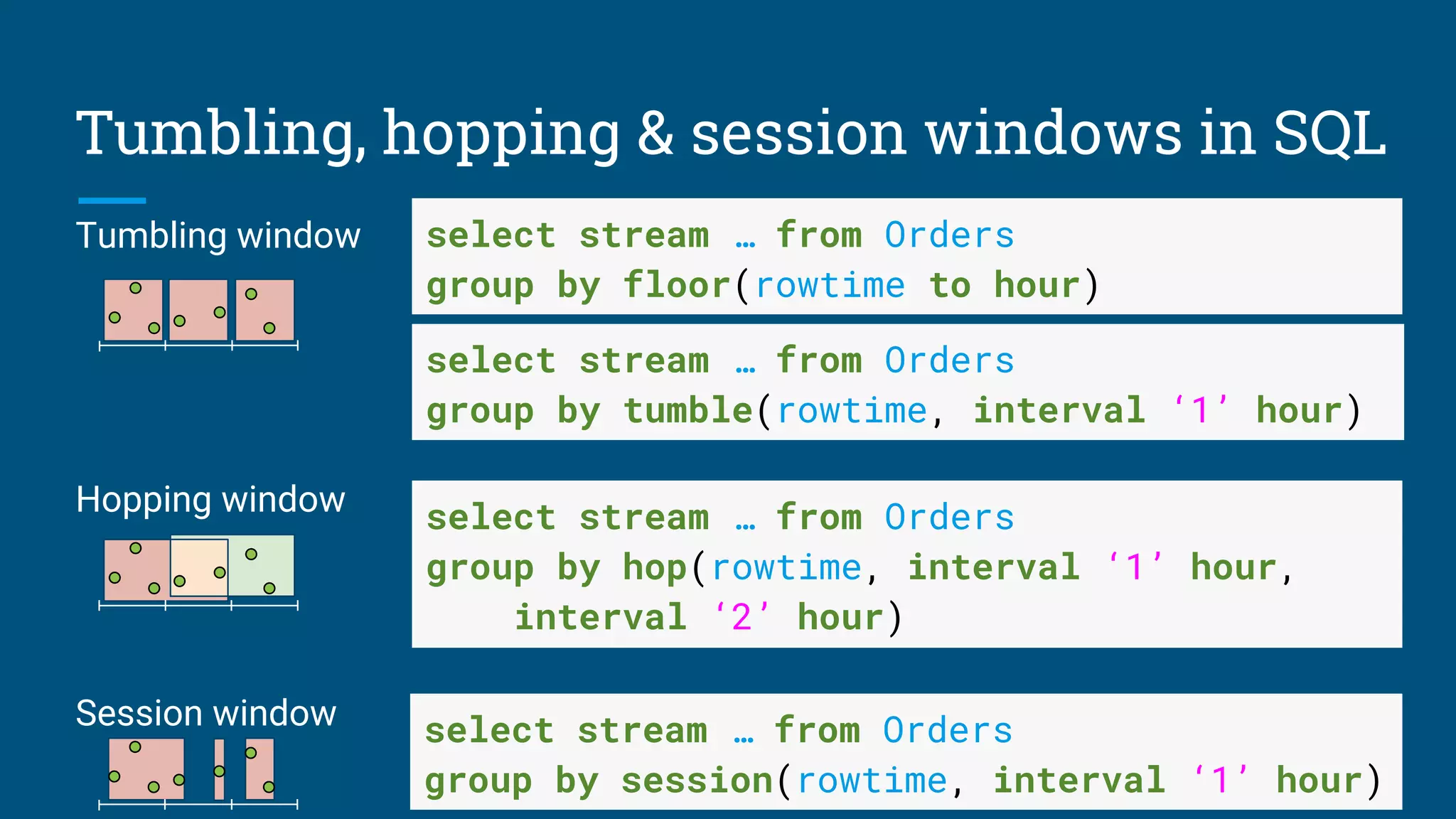
Core – Operator expressions
(relational algebra) and planner
(based on Volcano/Cascades[2])
External – Data storage, algorithms
and catalog
Optional – SQL parser, JDBC &
ODBC drivers
Extensible – Planner rewrite rules,
statistics, cost model, algebra, UDFs](https://image.slidesharecdn.com/calcite-lyft-2018-180628001402/75/Data-all-over-the-place-How-SQL-and-Apache-Calcite-bring-sanity-to-streaming-and-spatial-data-7-2048.jpg)
![Models of relations
A table is a multi-set of records; contents vary over time, with some kind
transactional consistency
A temporal table is like a table, but you can also query its contents at previous
times; usually mapped to a base table with (start, end) columns
So, what is a stream?
1. A stream is an append-only table with an event-time column
2. Or, if you speak monads[3], a stream is a function: Stream x → Time → Bag x
3. Or, a stream is the time-derivative of a table
Are a table, its temporal table, and its stream one catalog object or three?](https://image.slidesharecdn.com/calcite-lyft-2018-180628001402/75/Data-all-over-the-place-How-SQL-and-Apache-Calcite-bring-sanity-to-streaming-and-spatial-data-24-2048.jpg)
![Efficient spatial query?
Spatial queries are hard to execute efficiently.
Conventional DBs use two tricks that don’t work:
● Hash (no ranges / no locality)
● Sort (only one-dimensional ranges)
Two techniques that do work[4]:
● Data-organized structures (e.g. r-tree) – self-balancing
● Space-organized structures (e.g. tiles) – allow algebraic rewrite
Algebraic rewrites work on general-purpose data structures, and they compose.
•
•
•
•
A scan over a two-dimensional index only
has locality in one dimension](https://image.slidesharecdn.com/calcite-lyft-2018-180628001402/75/Data-all-over-the-place-How-SQL-and-Apache-Calcite-bring-sanity-to-streaming-and-spatial-data-31-2048.jpg)


![Architecture
Core – Operator expressions
(relational algebra) and planner
(based on Volcano/Cascades[2])
External – Data storage, algorithms
and catalog
Optional – SQL parser, JDBC &
ODBC drivers
Extensible – Planner rewrite rules,
statistics, cost model, algebra, UDFs](https://crownmelresort.com/image.slidesharecdn.com/calcite-lyft-2018-180628001402/75/Data-all-over-the-place-How-SQL-and-Apache-Calcite-bring-sanity-to-streaming-and-spatial-data-7-2048.jpg)


![Models of relations
A table is a multi-set of records; contents vary over time, with some kind
transactional consistency
A temporal table is like a table, but you can also query its contents at previous
times; usually mapped to a base table with (start, end) columns
So, what is a stream?
1. A stream is an append-only table with an event-time column
2. Or, if you speak monads[3], a stream is a function: Stream x → Time → Bag x
3. Or, a stream is the time-derivative of a table
Are a table, its temporal table, and its stream one catalog object or three?](https://crownmelresort.com/image.slidesharecdn.com/calcite-lyft-2018-180628001402/75/Data-all-over-the-place-How-SQL-and-Apache-Calcite-bring-sanity-to-streaming-and-spatial-data-24-2048.jpg)


![Efficient spatial query?
Spatial queries are hard to execute efficiently.
Conventional DBs use two tricks that don’t work:
● Hash (no ranges / no locality)
● Sort (only one-dimensional ranges)
Two techniques that do work[4]:
● Data-organized structures (e.g. r-tree) – self-balancing
● Space-organized structures (e.g. tiles) – allow algebraic rewrite
Algebraic rewrites work on general-purpose data structures, and they compose.
•
•
•
•
A scan over a two-dimensional index only
has locality in one dimension](https://crownmelresort.com/image.slidesharecdn.com/calcite-lyft-2018-180628001402/75/Data-all-over-the-place-How-SQL-and-Apache-Calcite-bring-sanity-to-streaming-and-spatial-data-31-2048.jpg)


The document discusses Apache Calcite, a framework that brings order to diverse data formats and enables efficient query processing across streaming, spatial, and relational data. It outlines key features of Calcite, including query federation, materialized views, and SQL syntax extensions for streaming queries. The presentation emphasizes the importance of SQL as a standardized language for handling various data paradigms in modern enterprises.
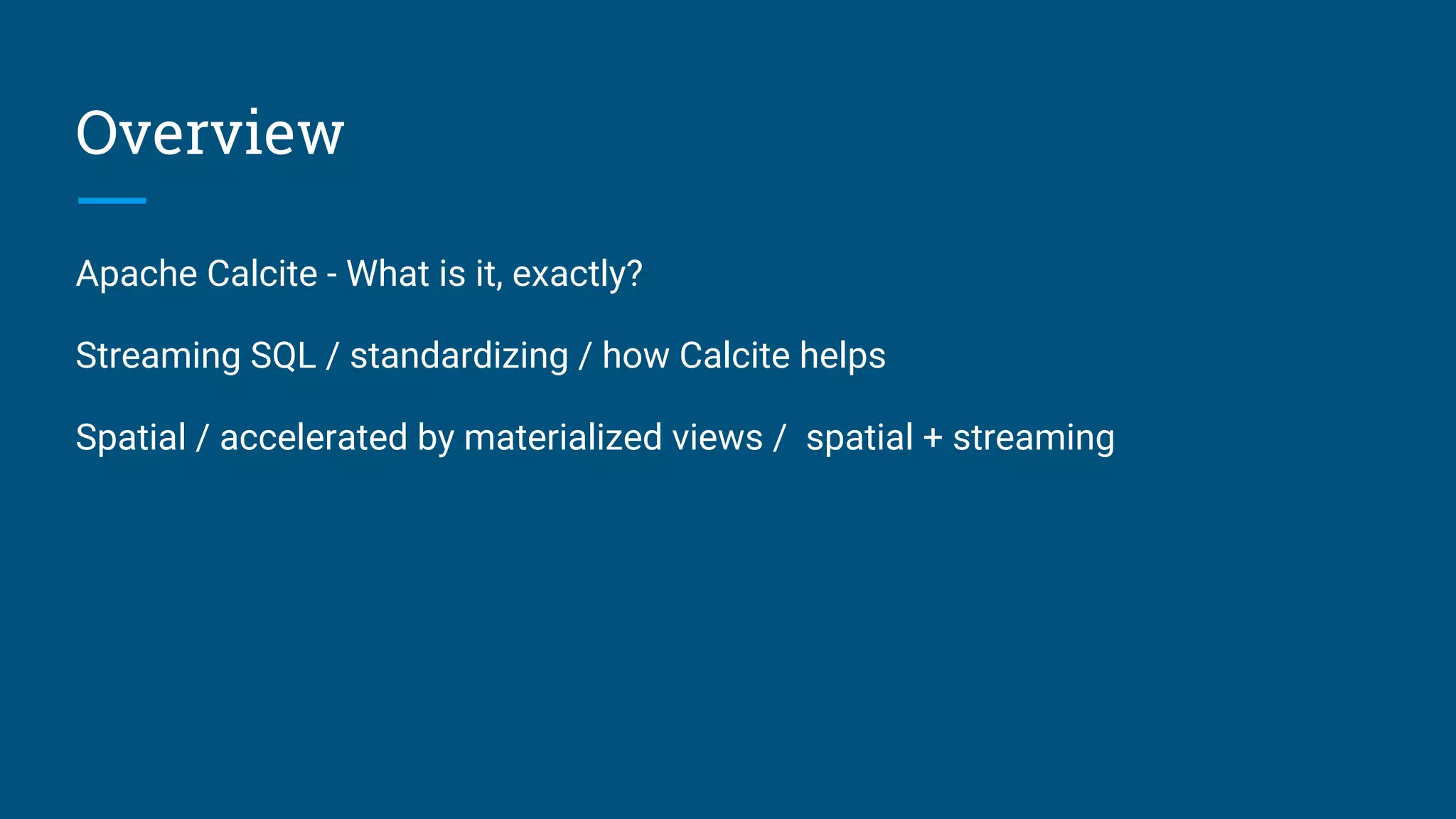
Introduction to Apache Calcite and its purpose in standardizing streaming and spatial data.
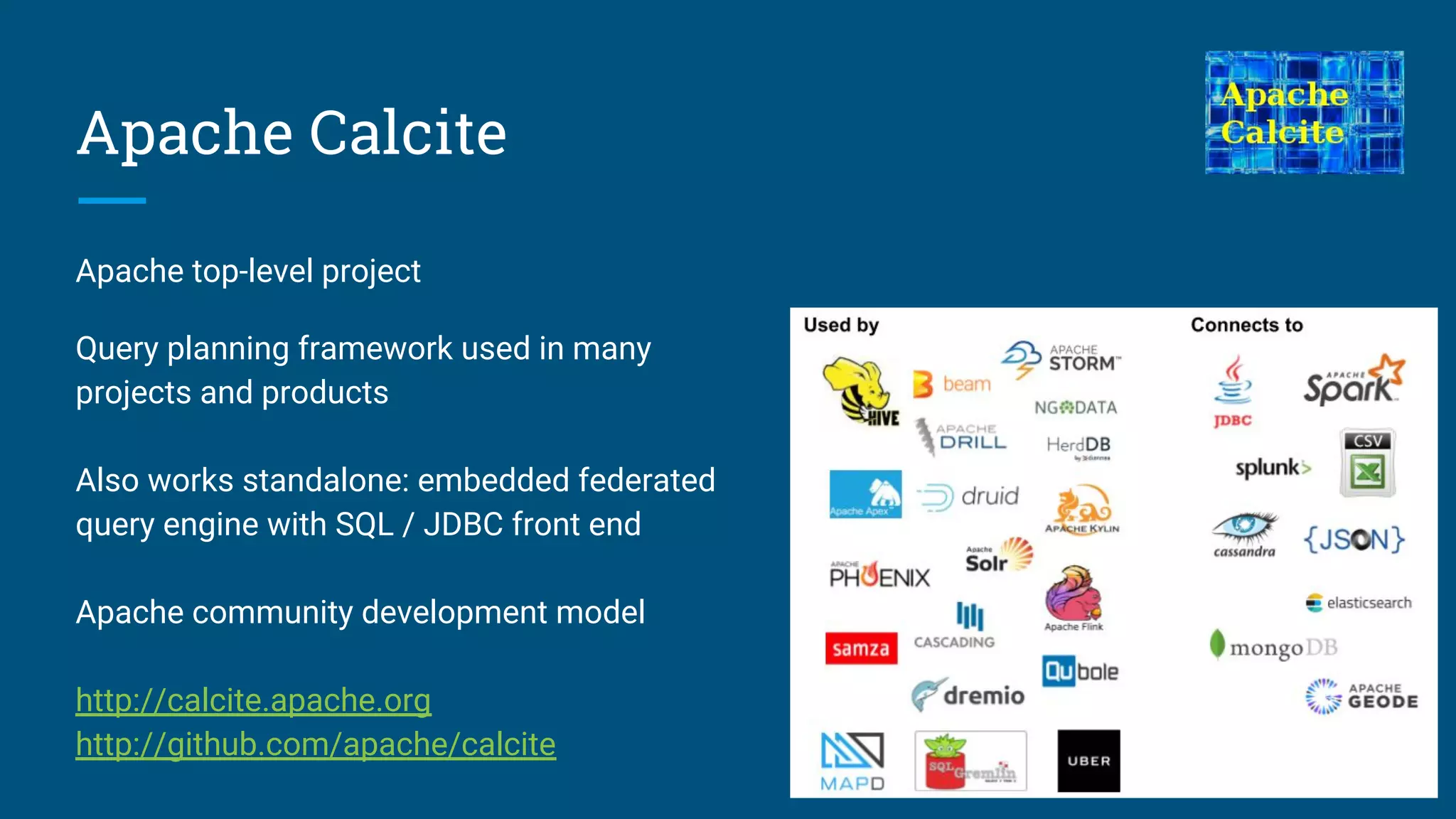
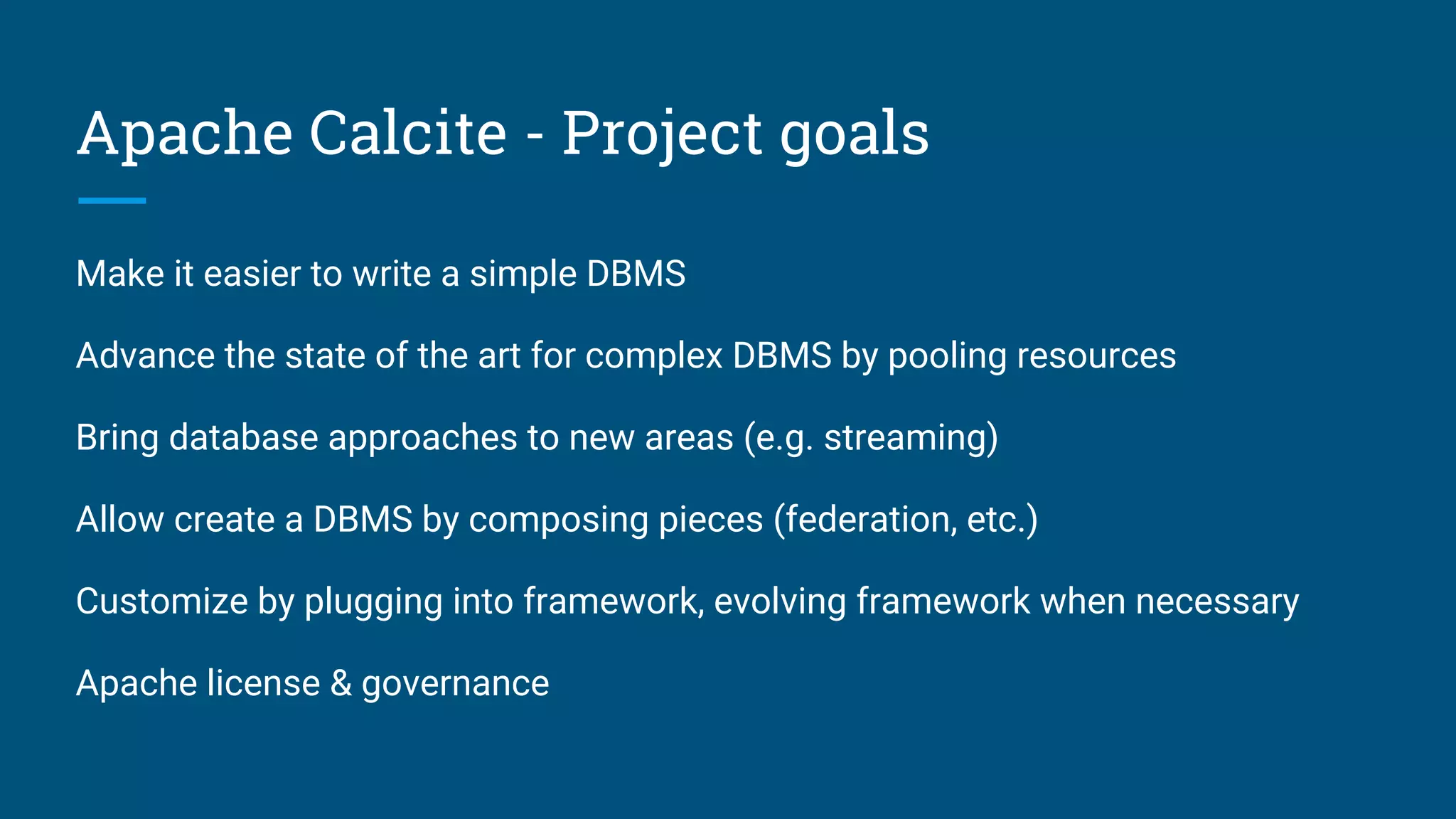
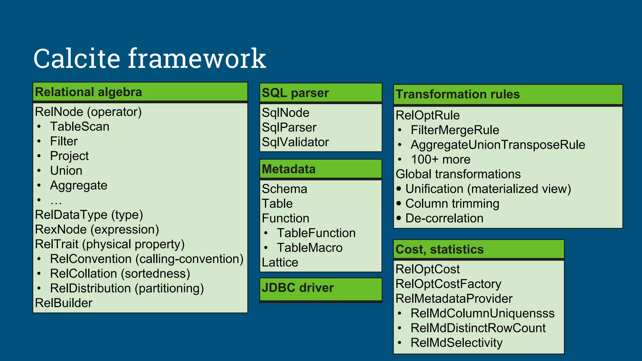
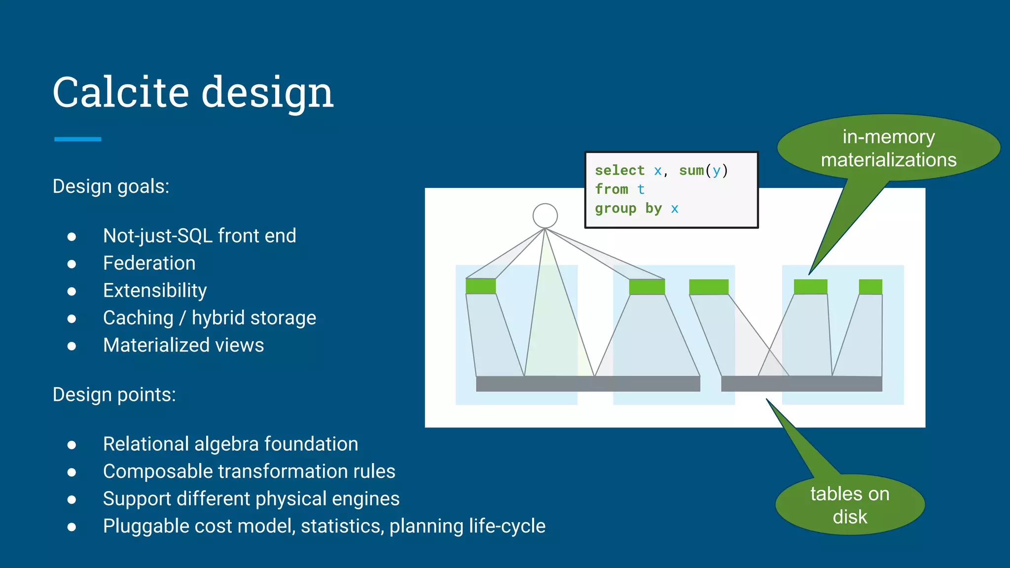
Details on Apache Calcite, goals, and its architecture as a query planning framework.
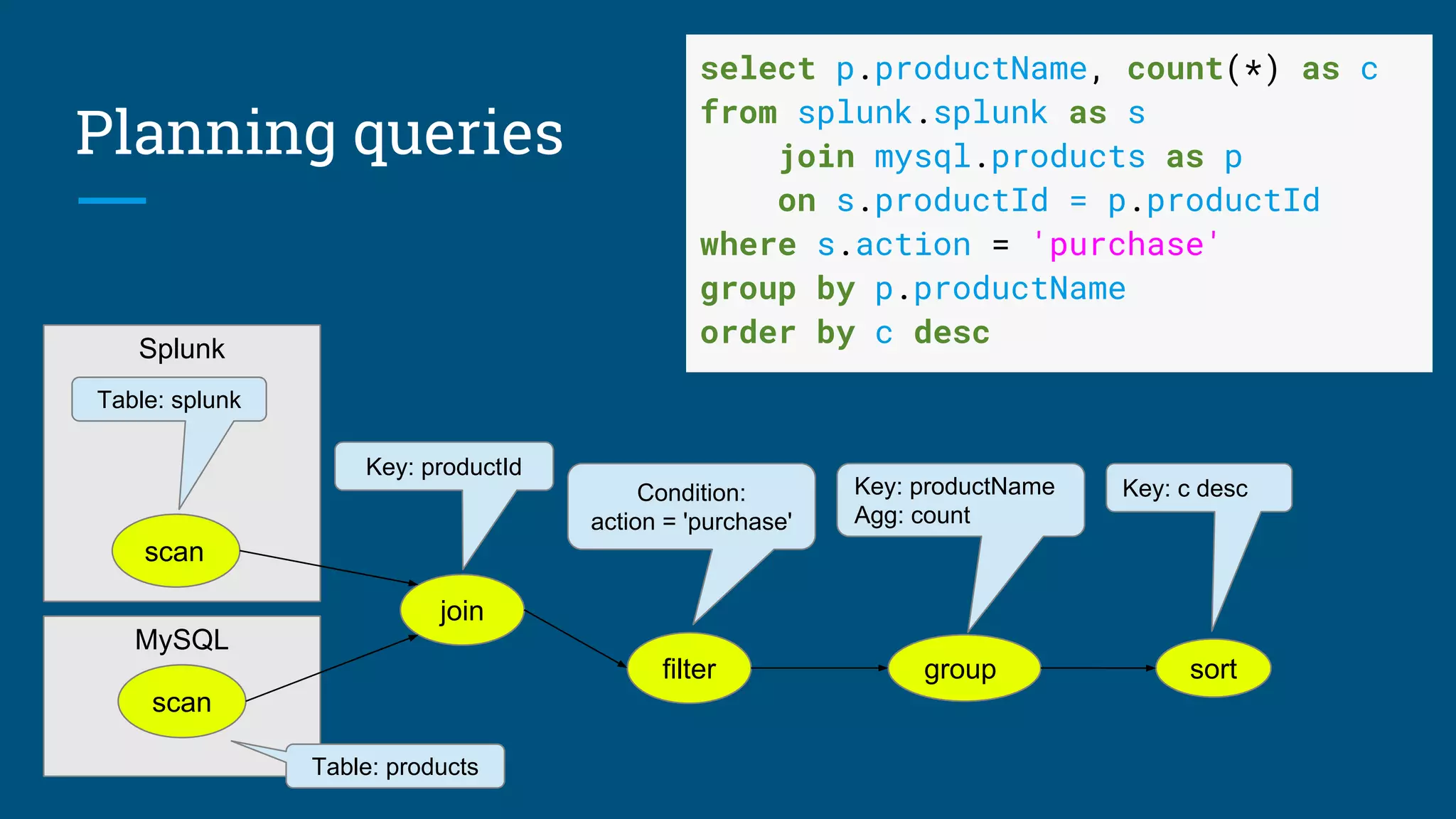
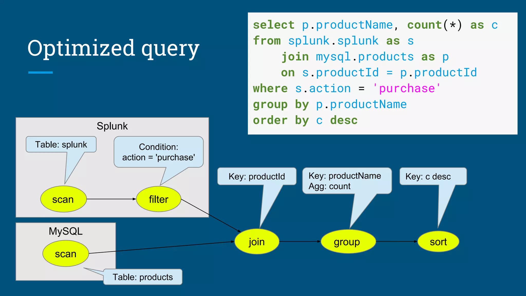
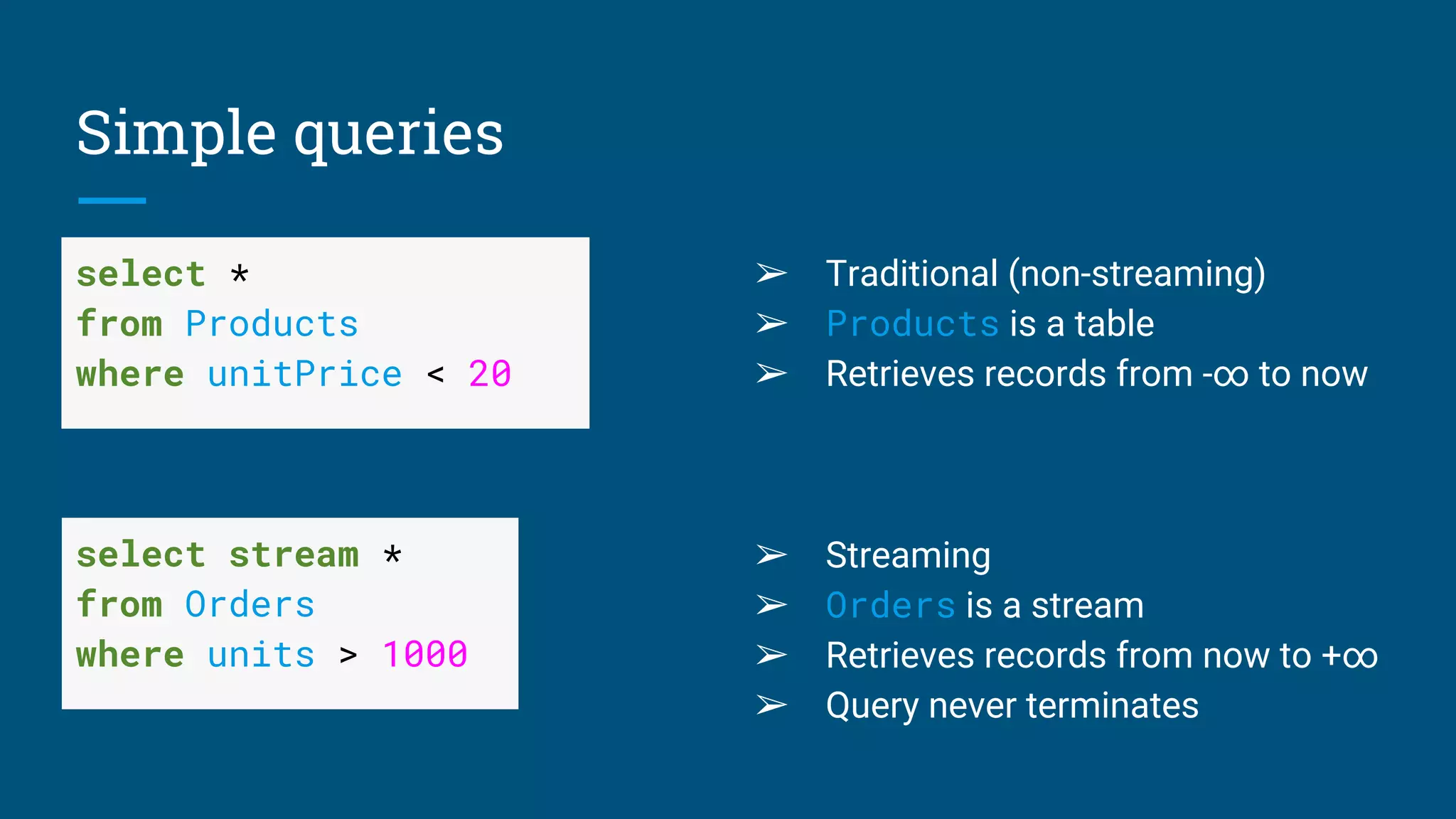
Sample SQL queries illustrating query planning with Apache Calcite and optimization techniques.
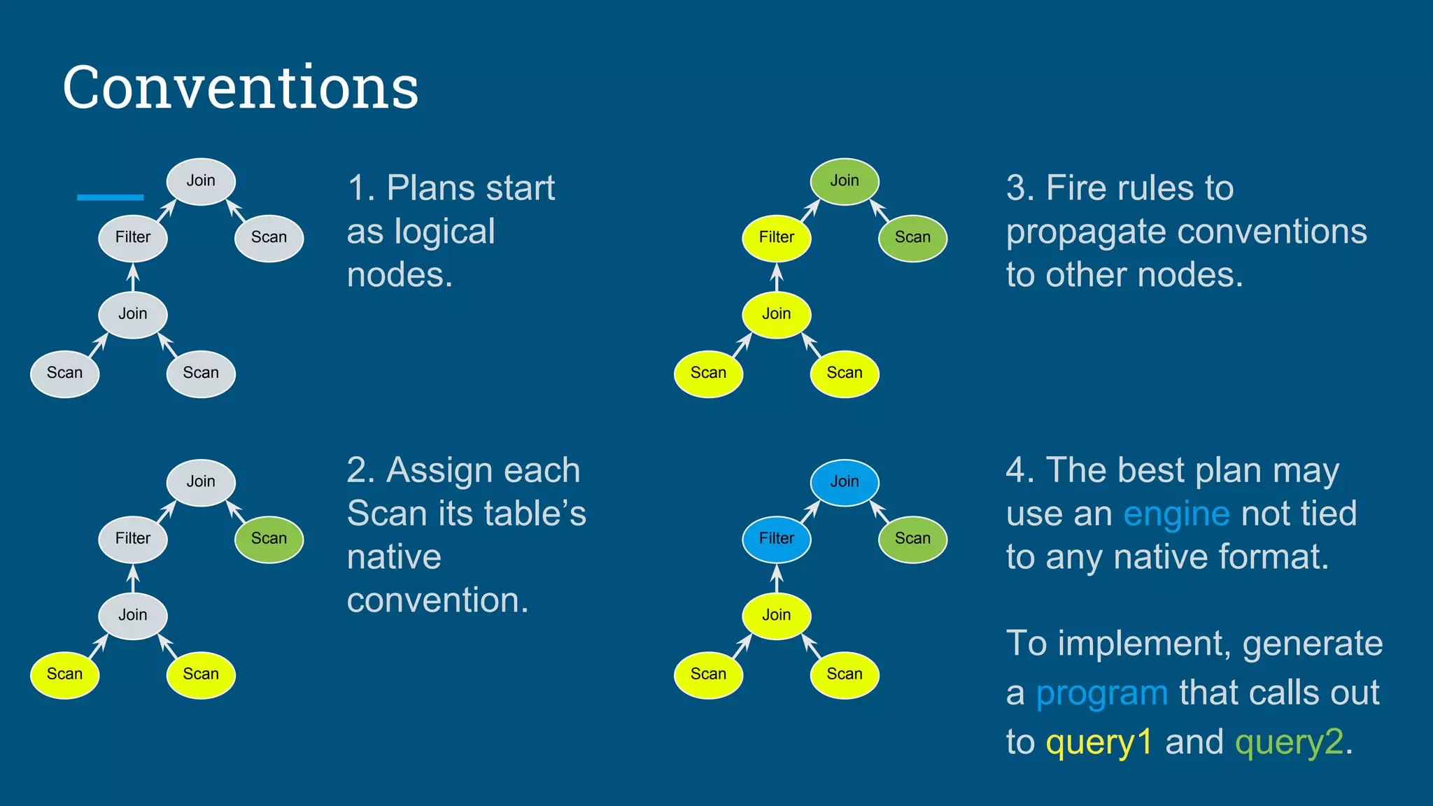
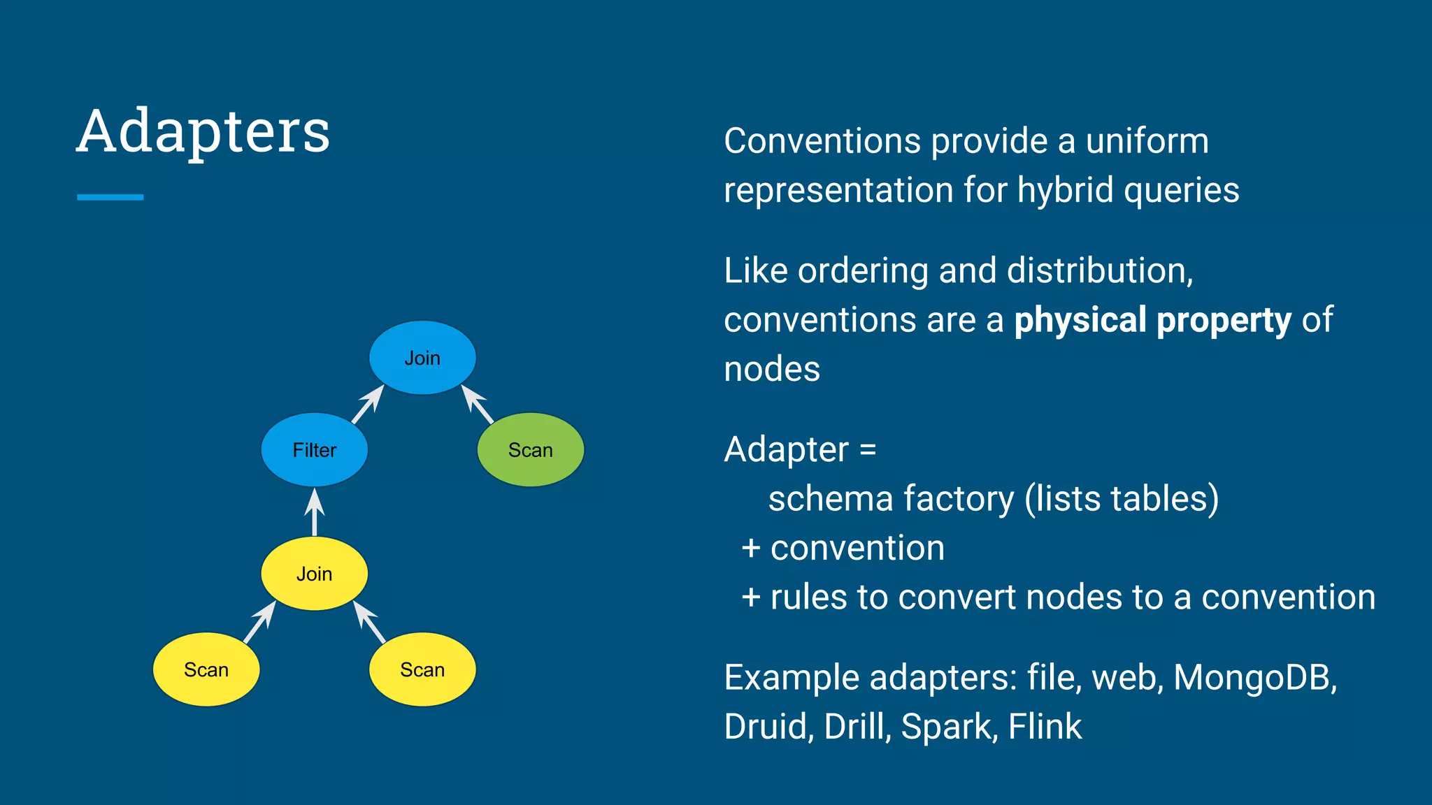
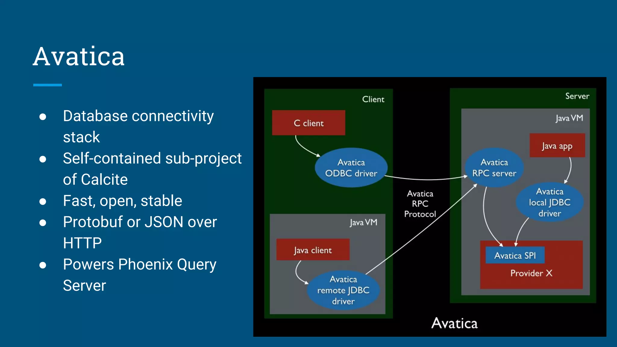
Execution flow of queries and explanations of adapters that translate data sources.
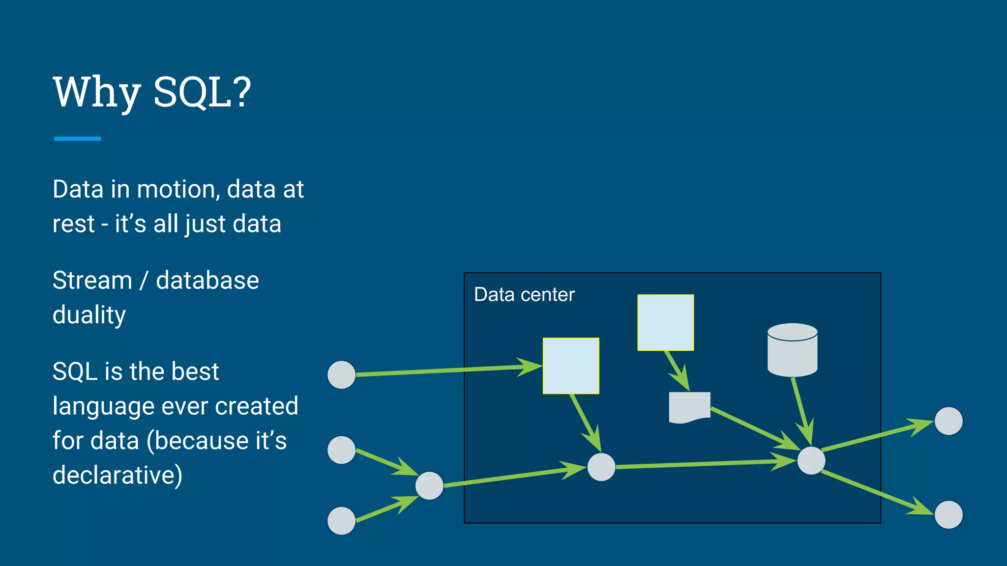
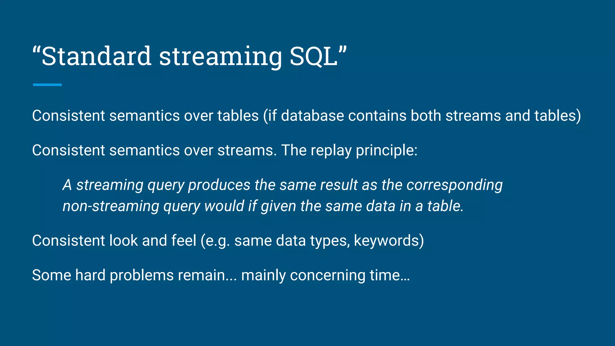
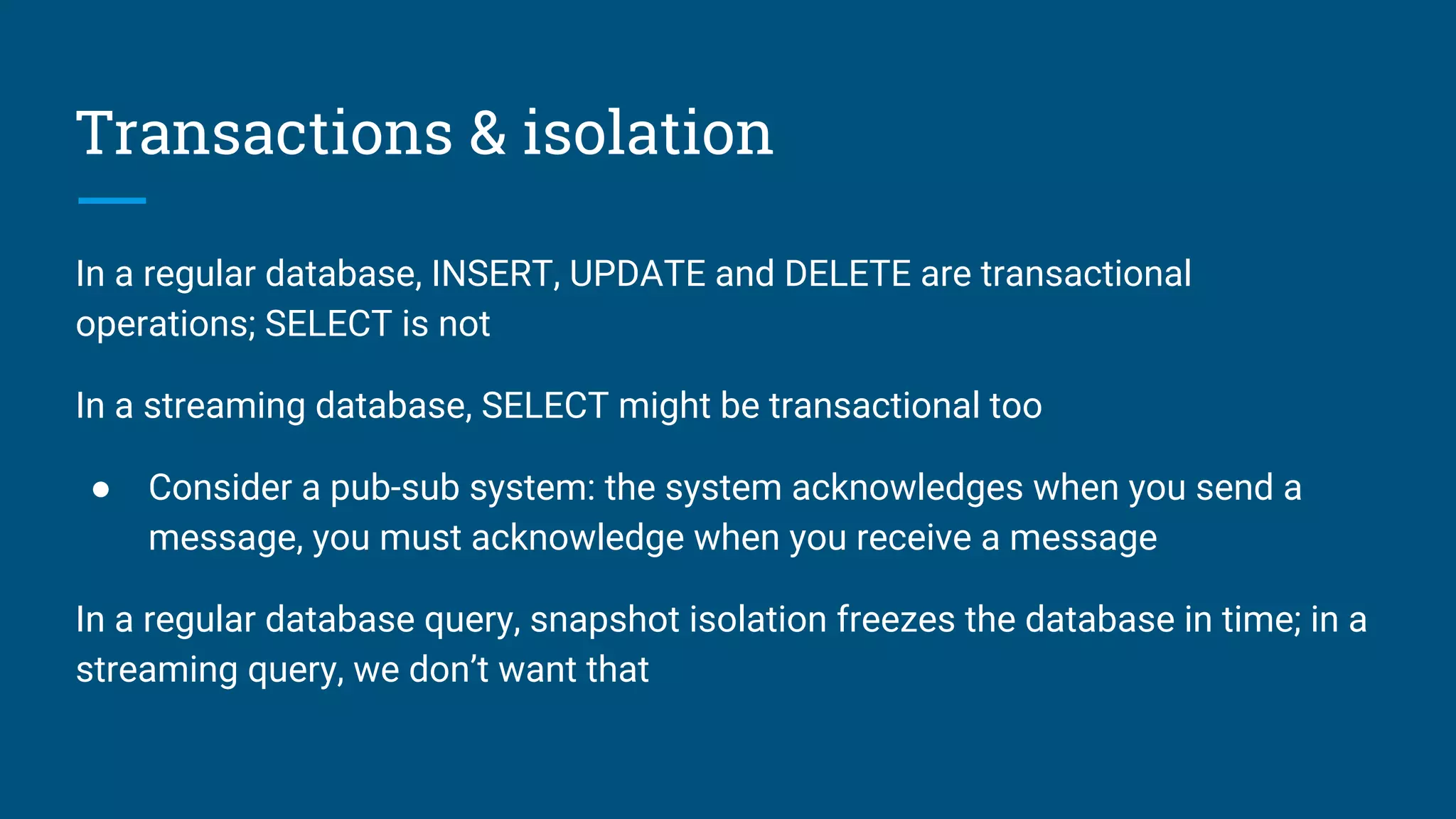
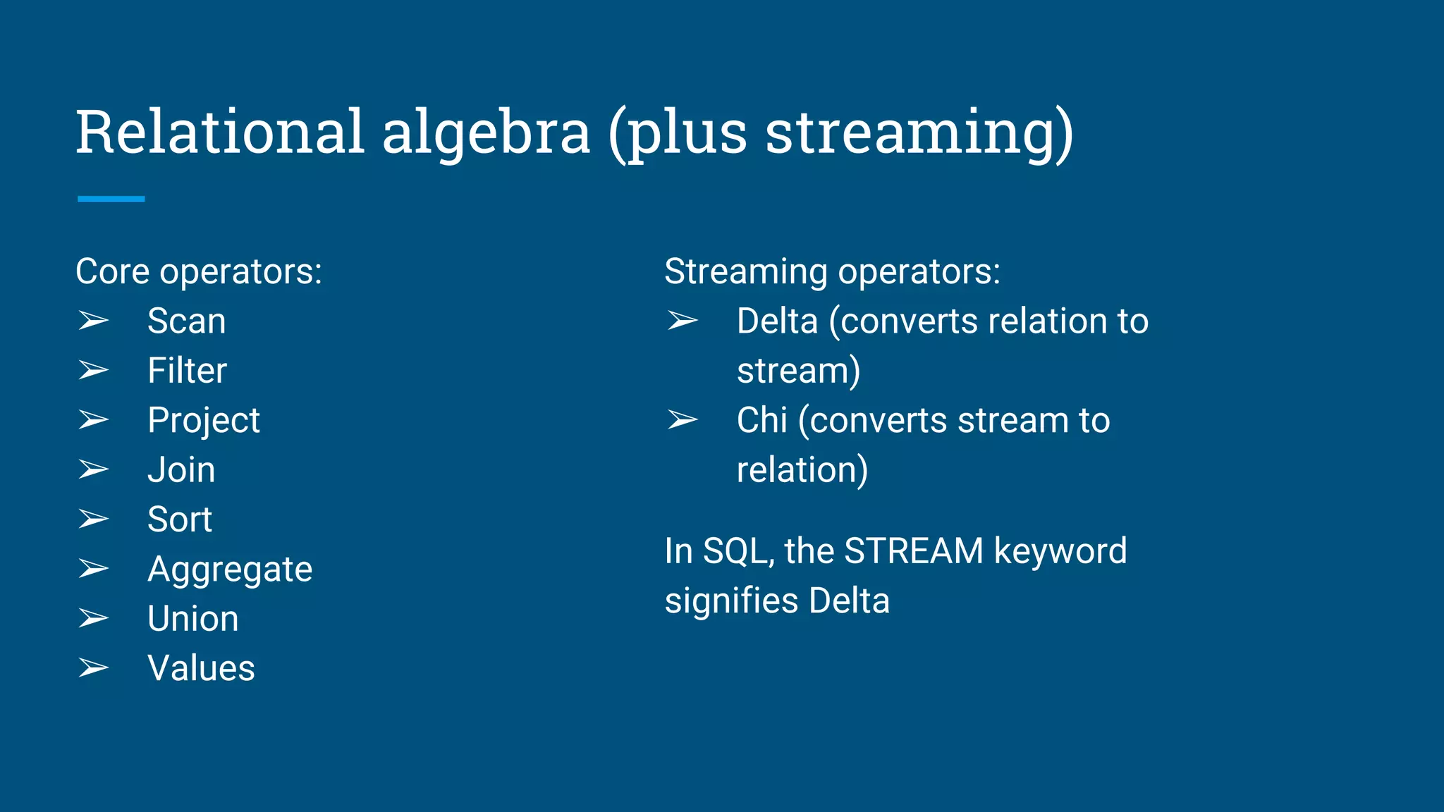
Introduction to streaming SQL and the reasons for using SQL in both streaming and traditional databases.
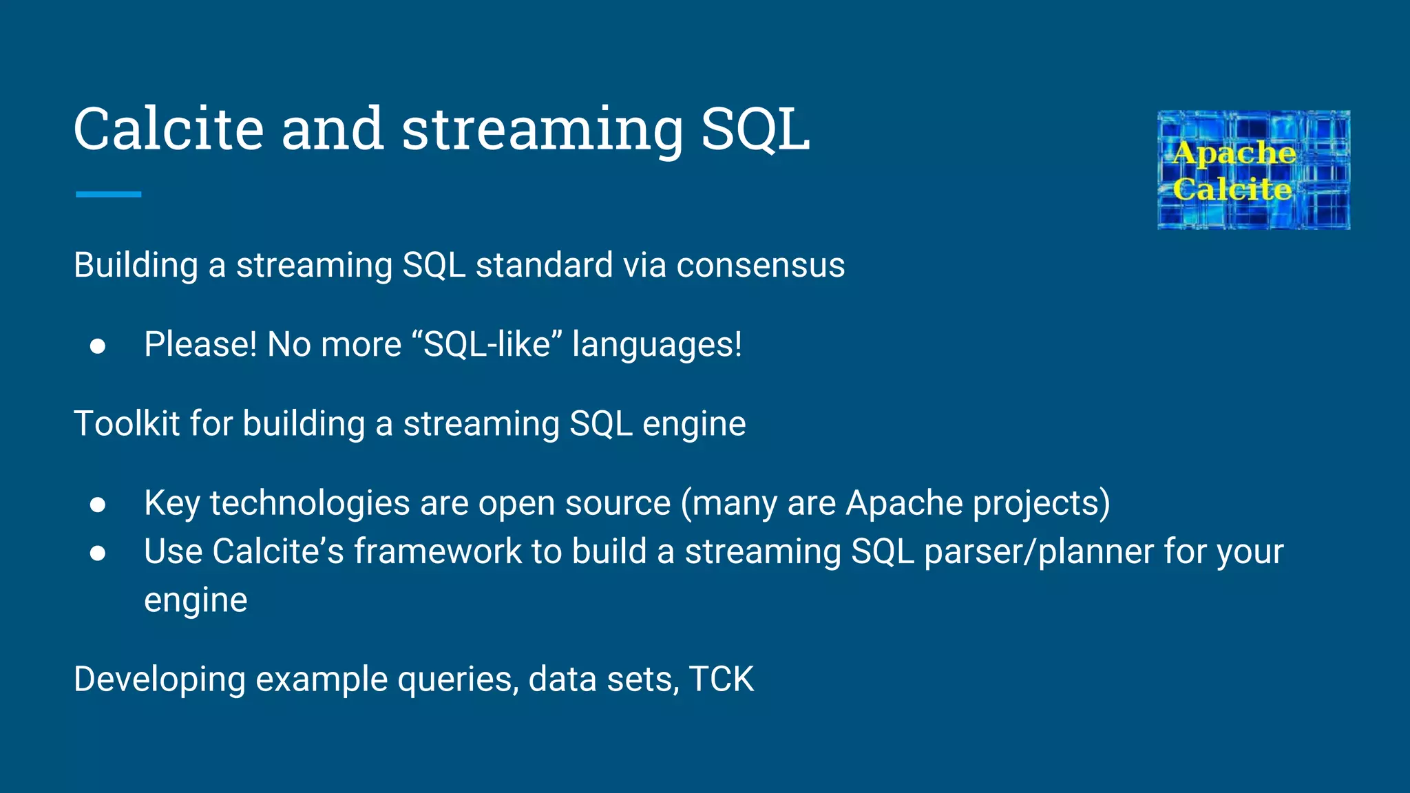
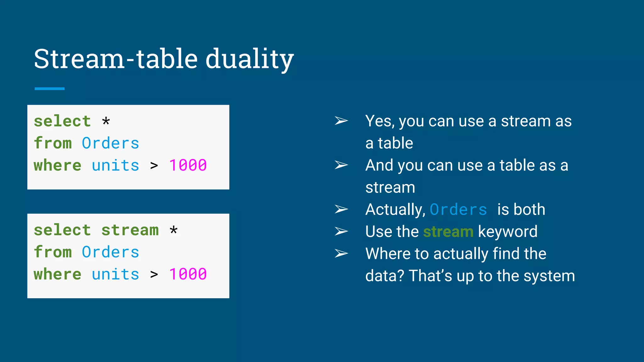
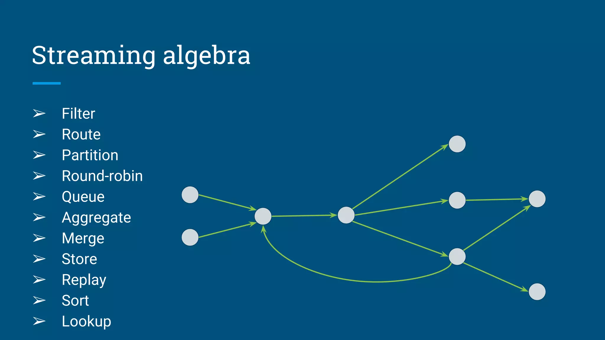
Framework for developing a consistent streaming SQL standard, emphasizing duality of streams and tables.
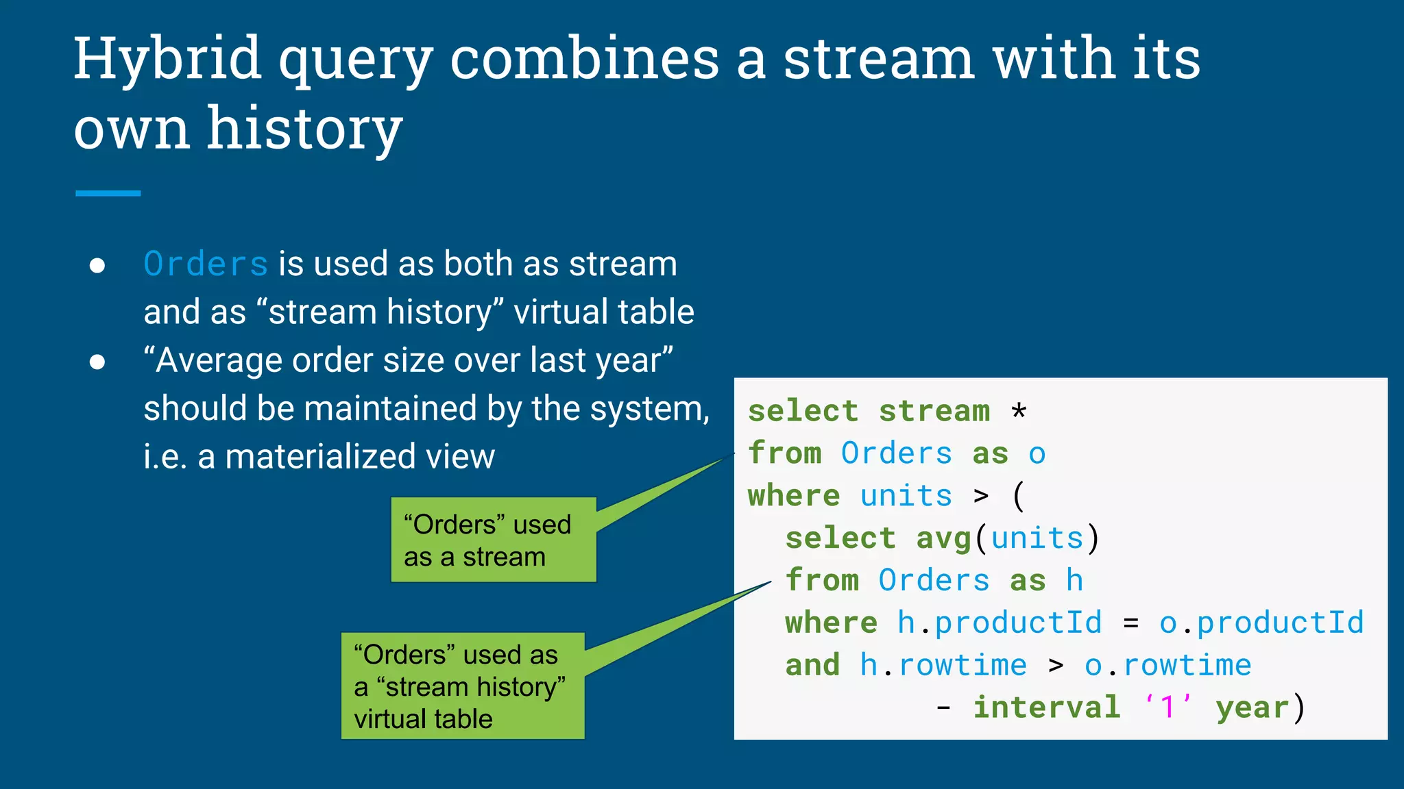
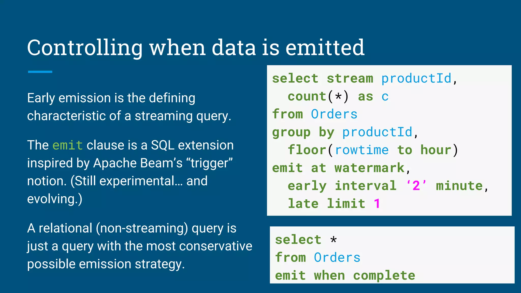
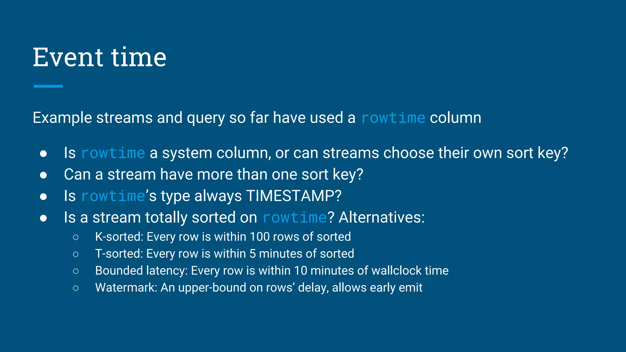
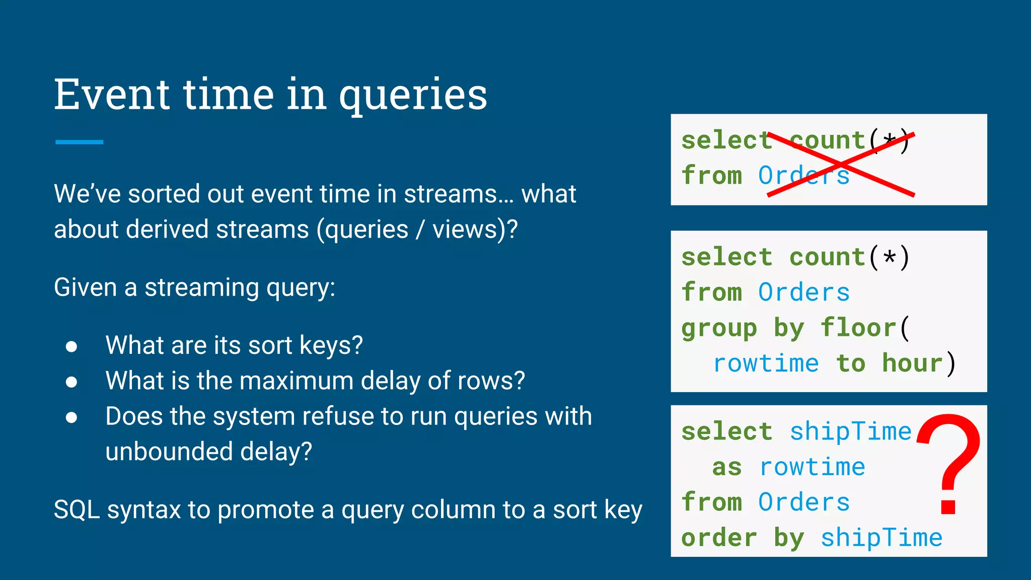
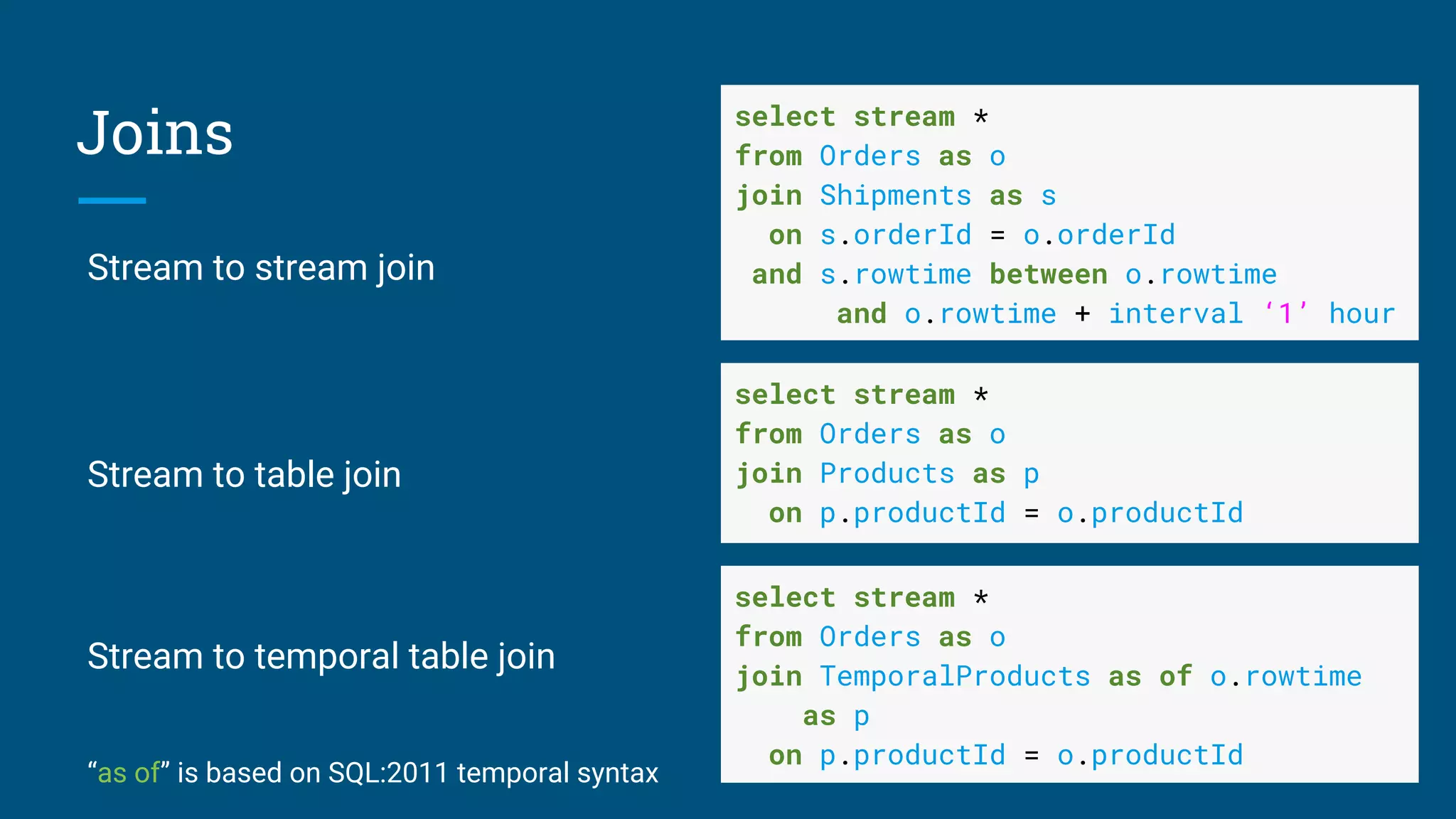
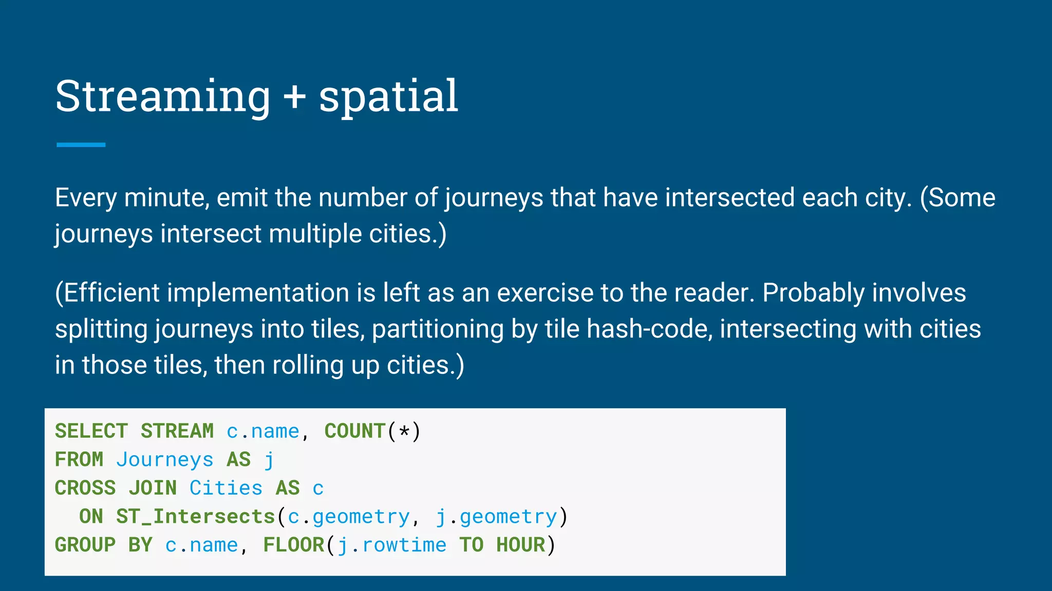
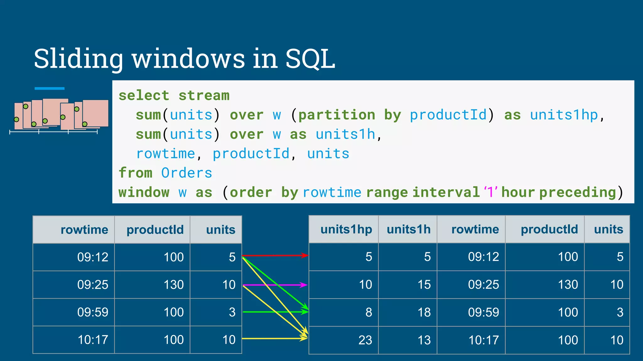
Details on emitting data, event time management, combining stream and temporal tables with SQL.
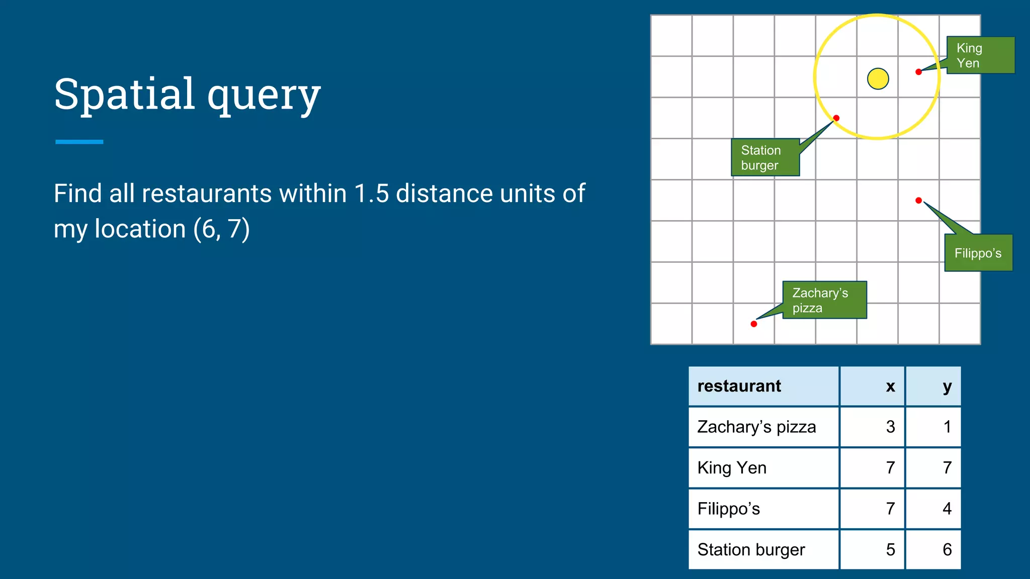
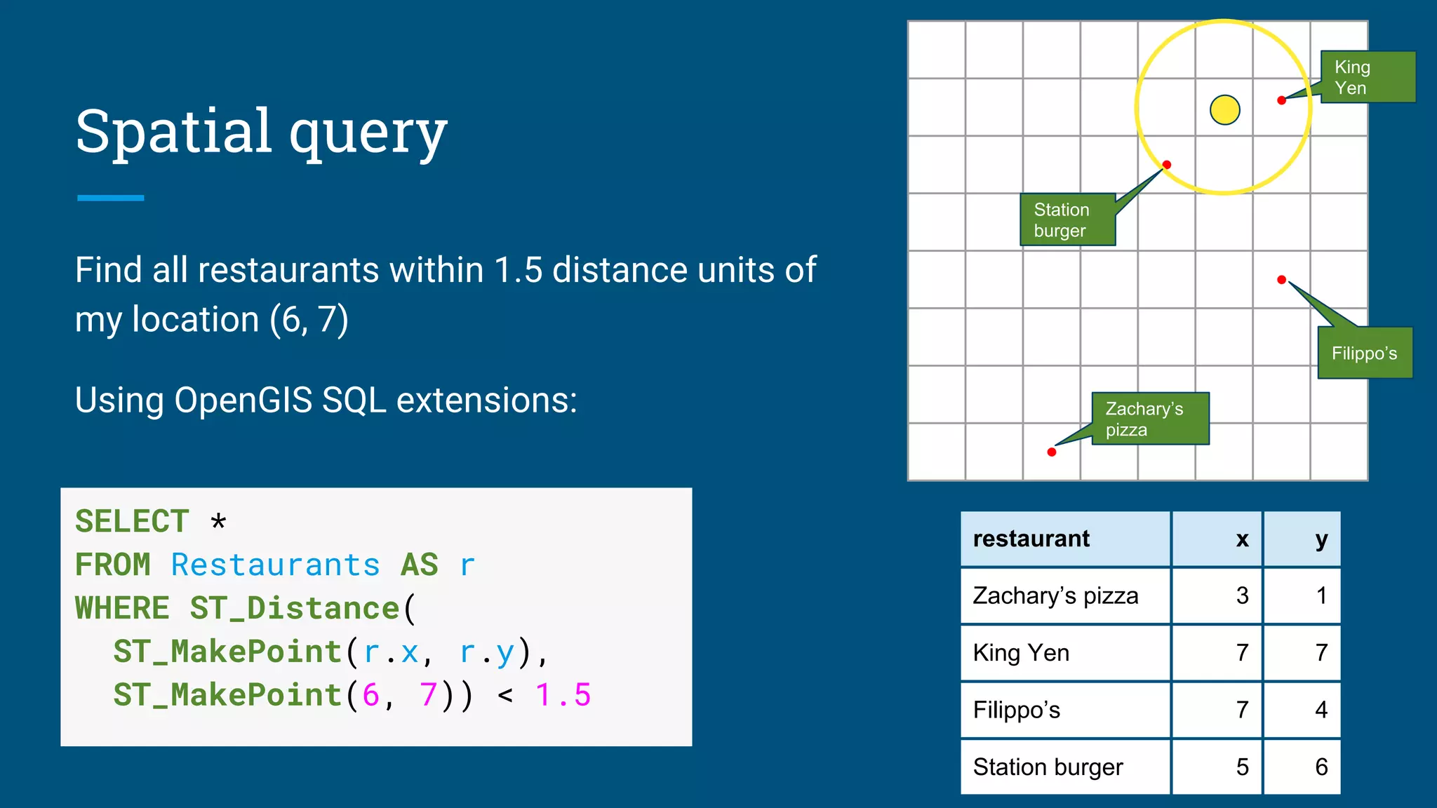
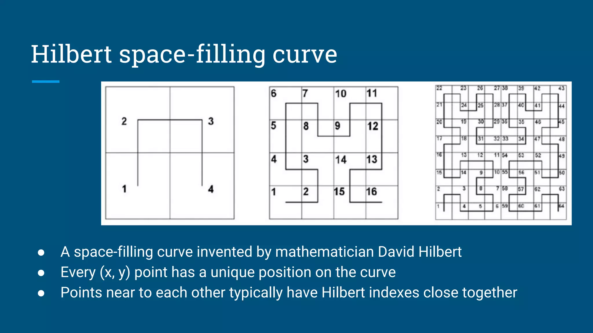
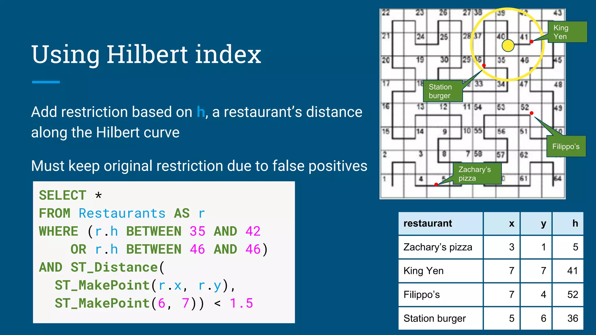
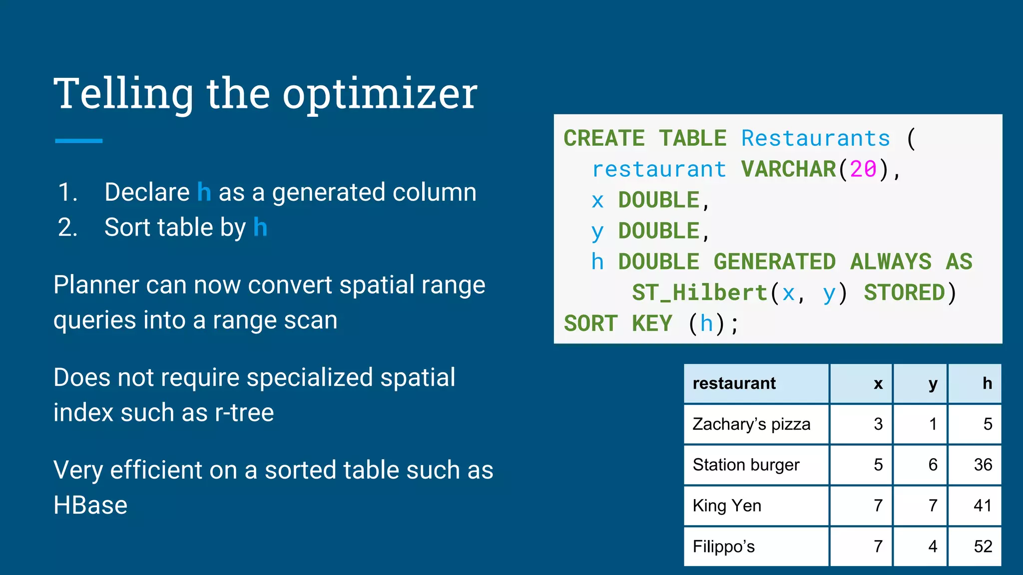
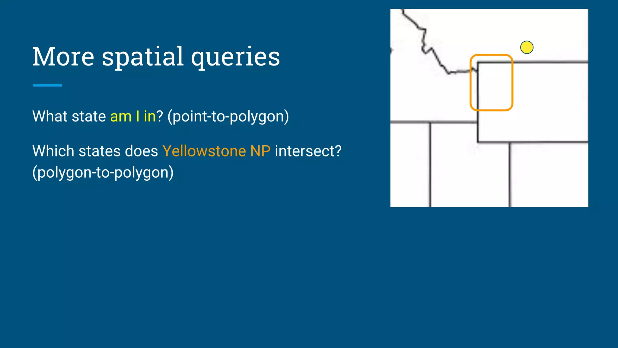
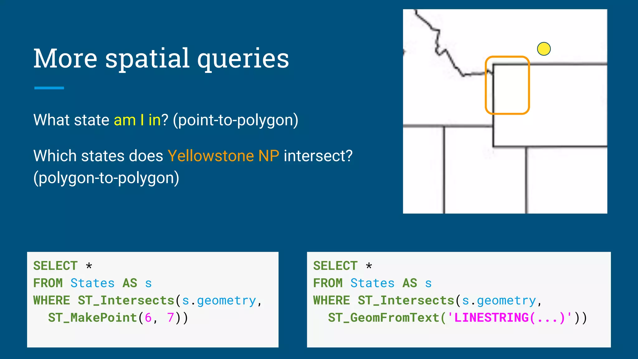
Introduction to spatial queries using geographic data and techniques for optimizing spatial queries.
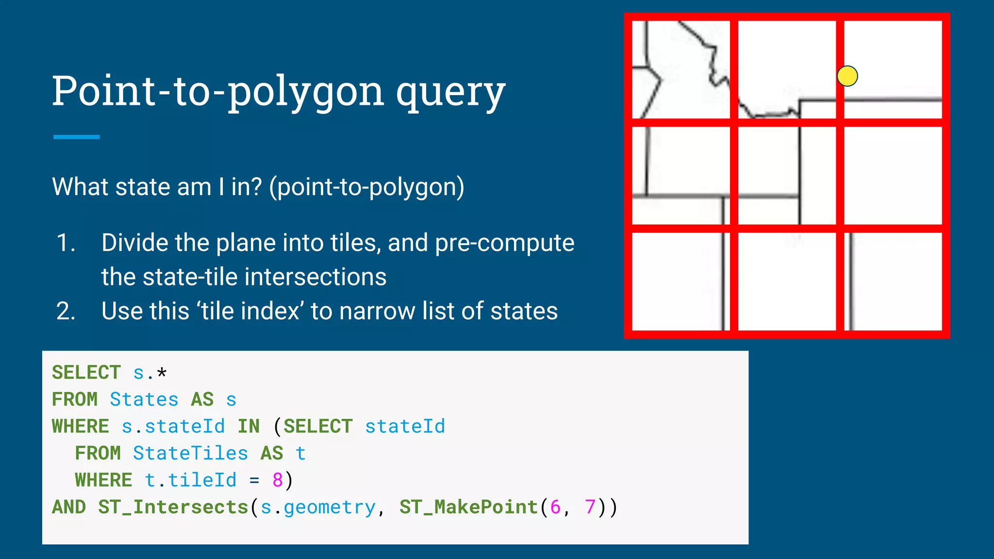
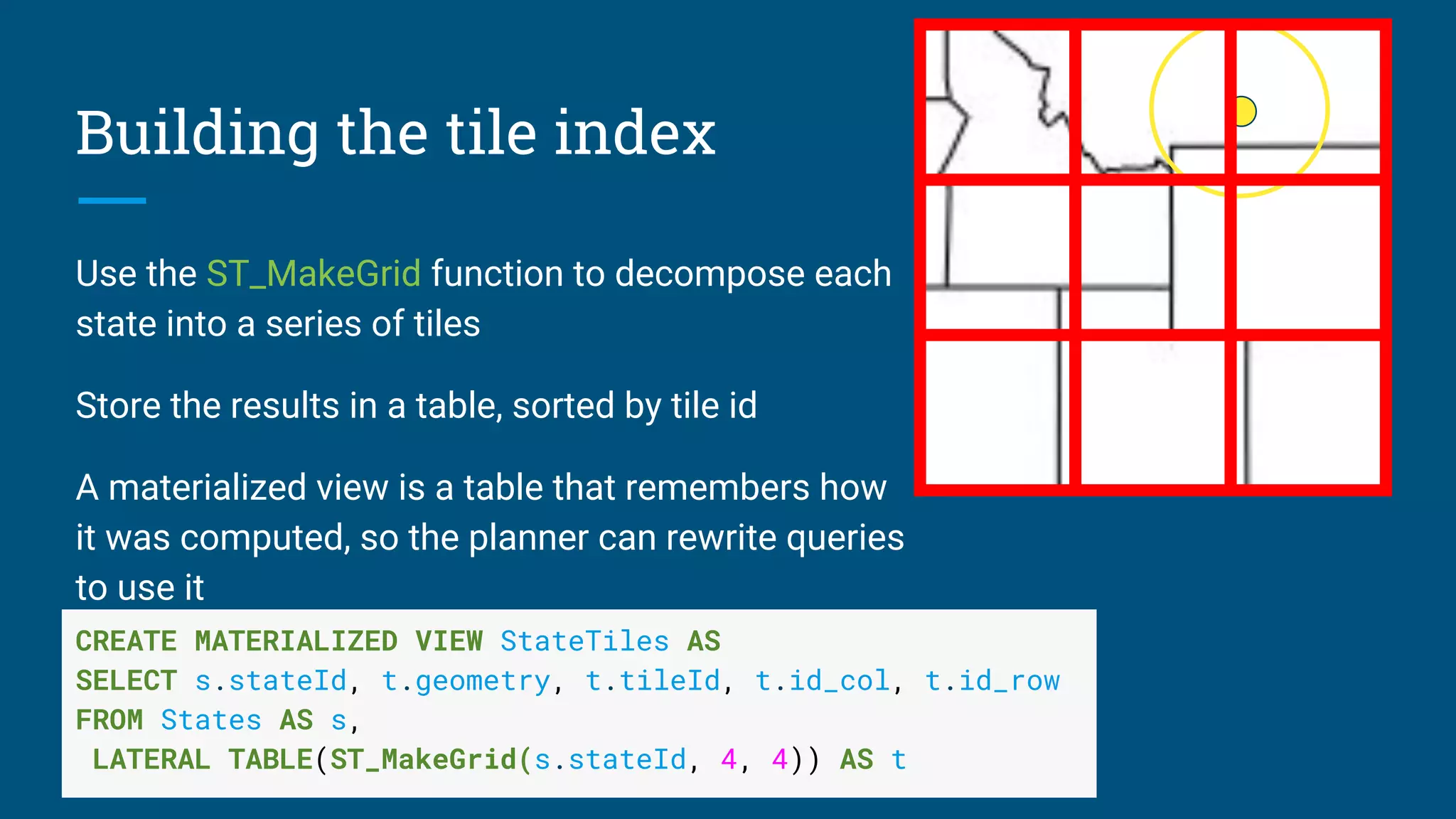
Examples of complex spatial queries including point-to-polygon and utilizing materialized views.
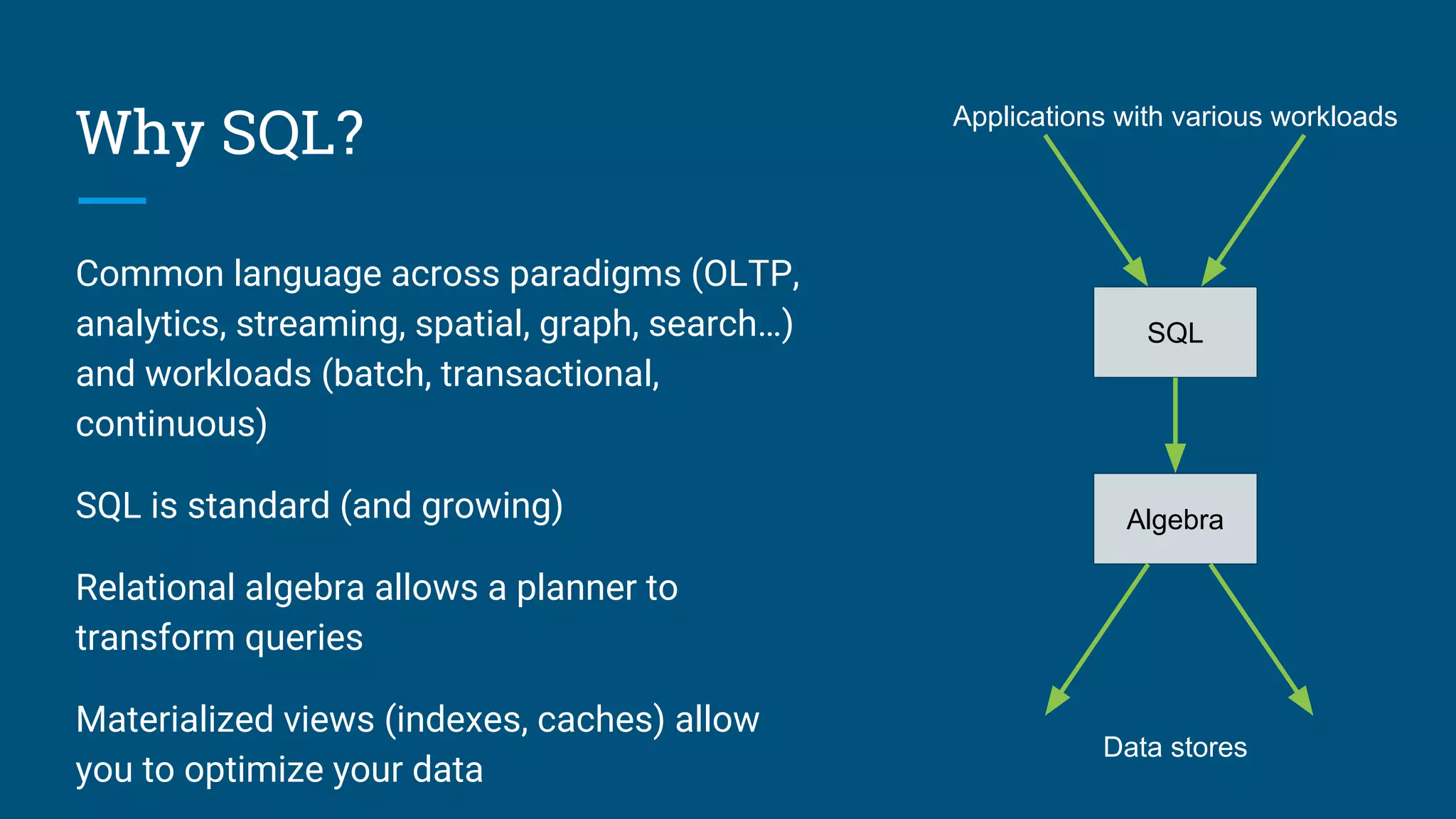
Summary of SQL's role as a common language across various data paradigms and workloads.
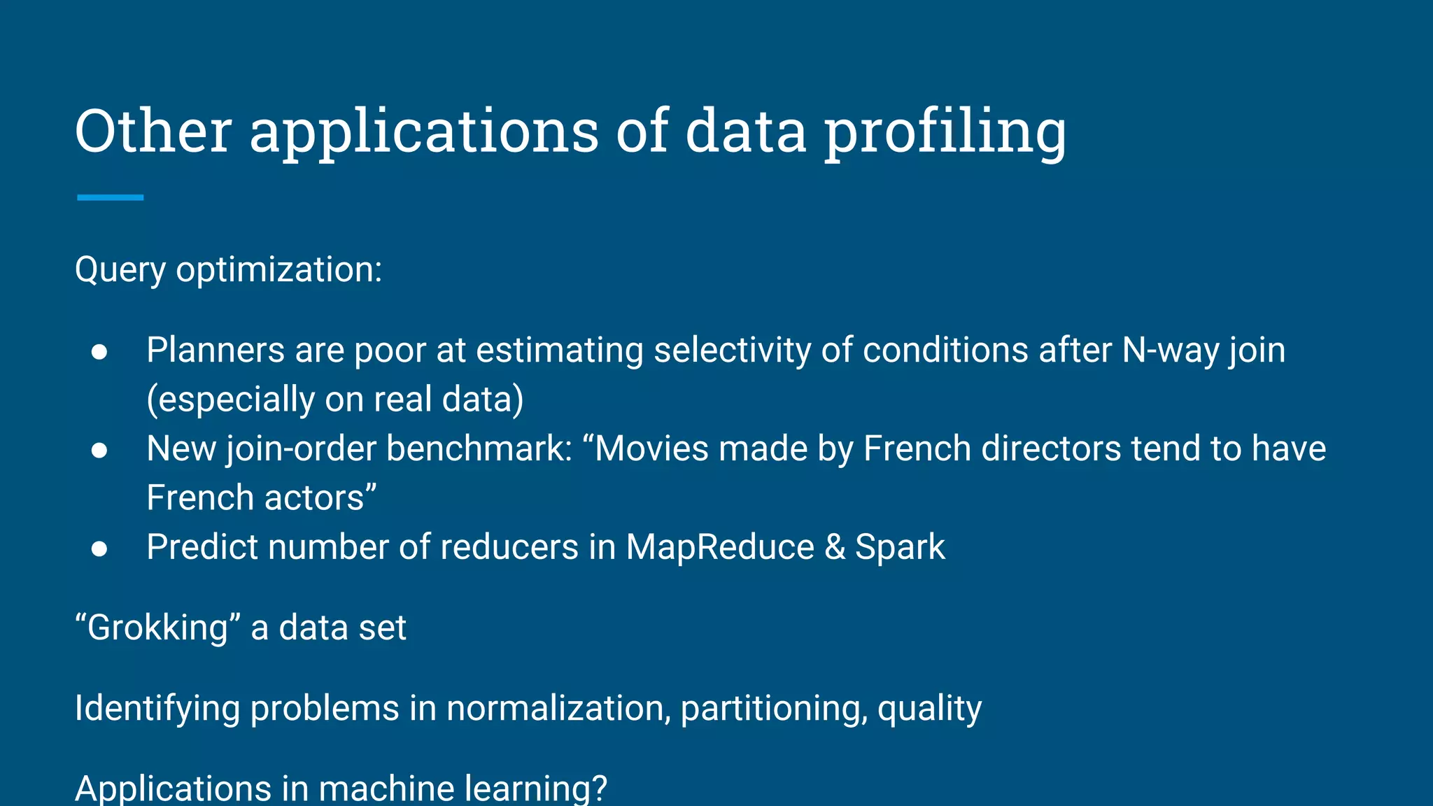
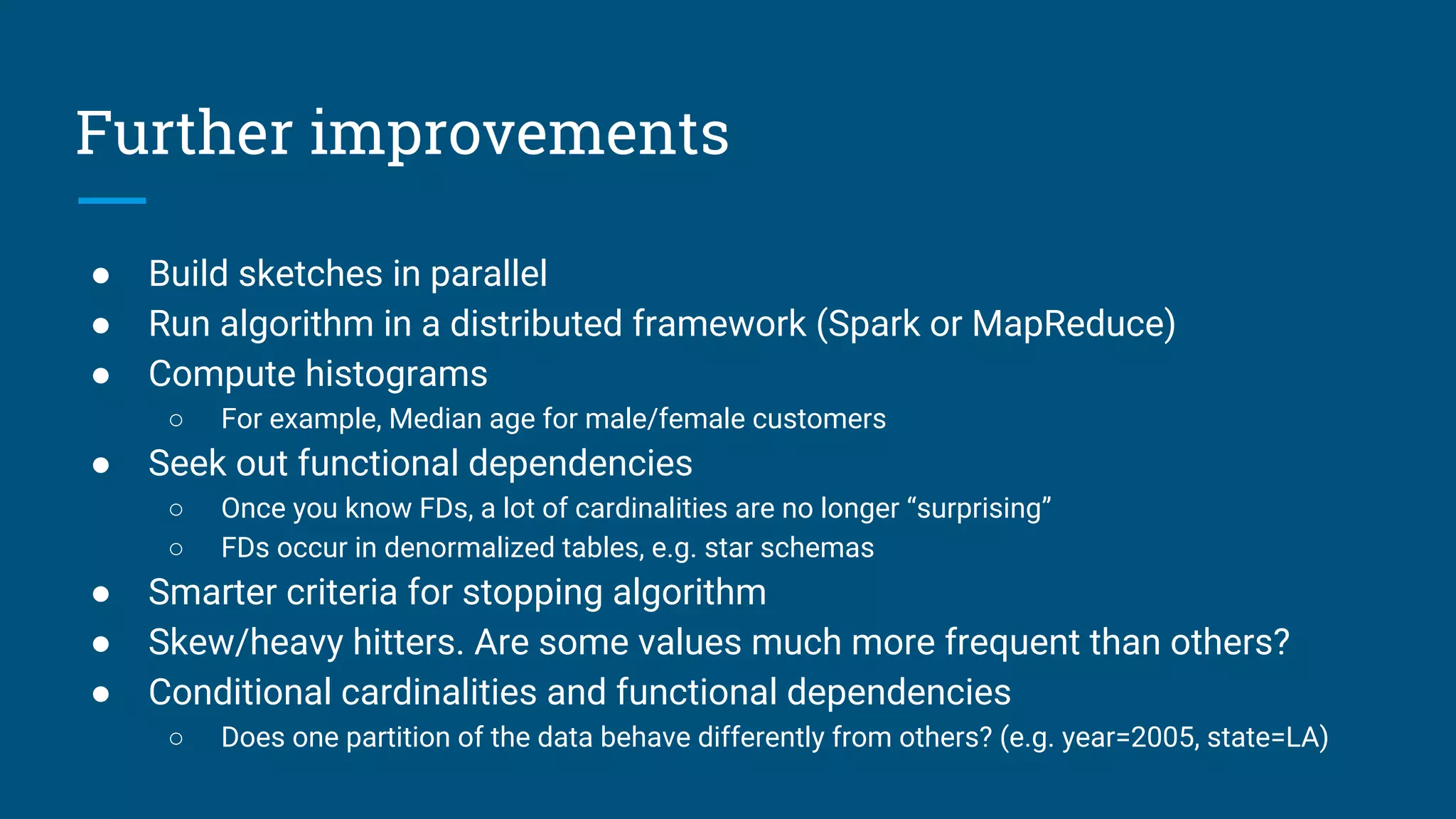
Applications of data profiling, query optimization, and relational algebra in contexts beyond traditional queries.
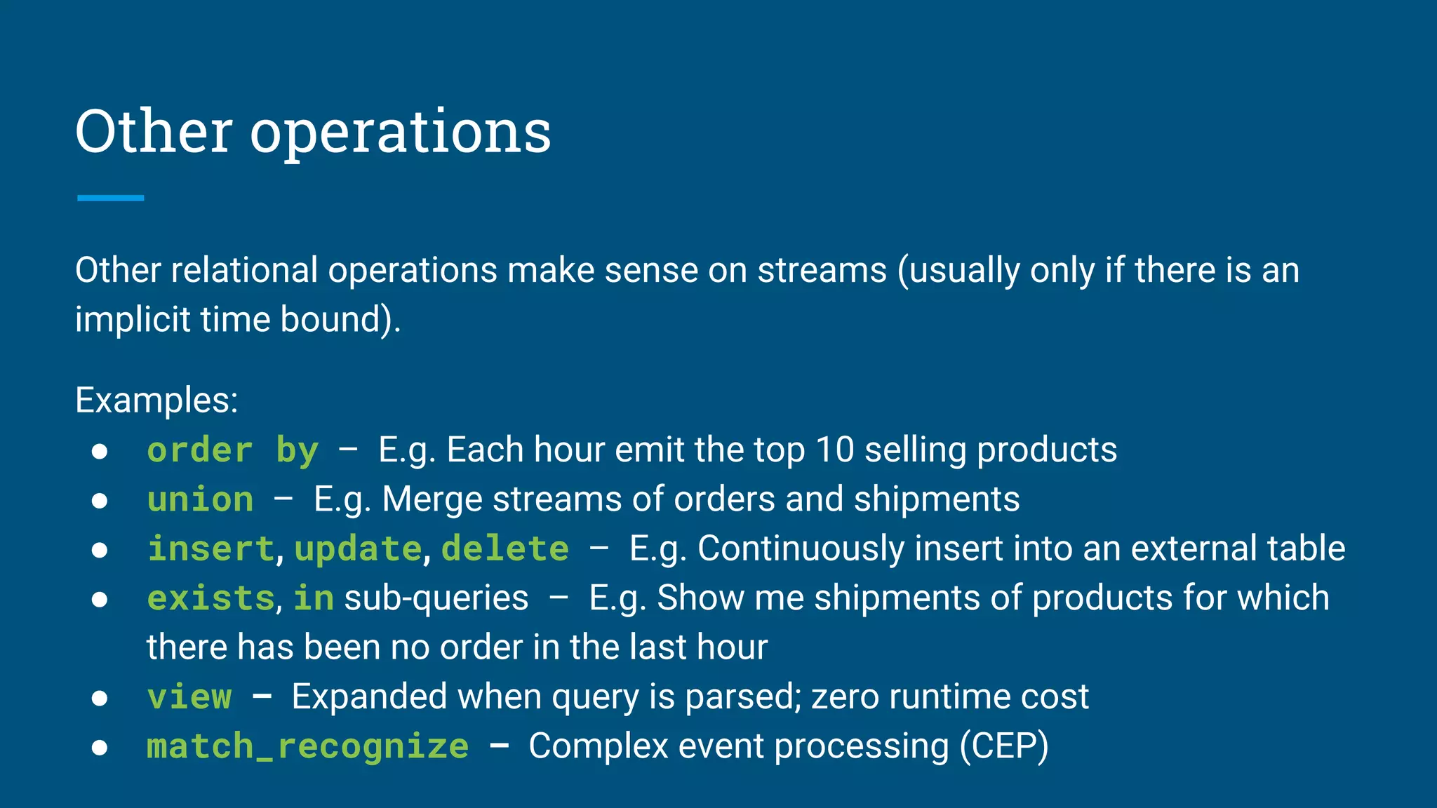
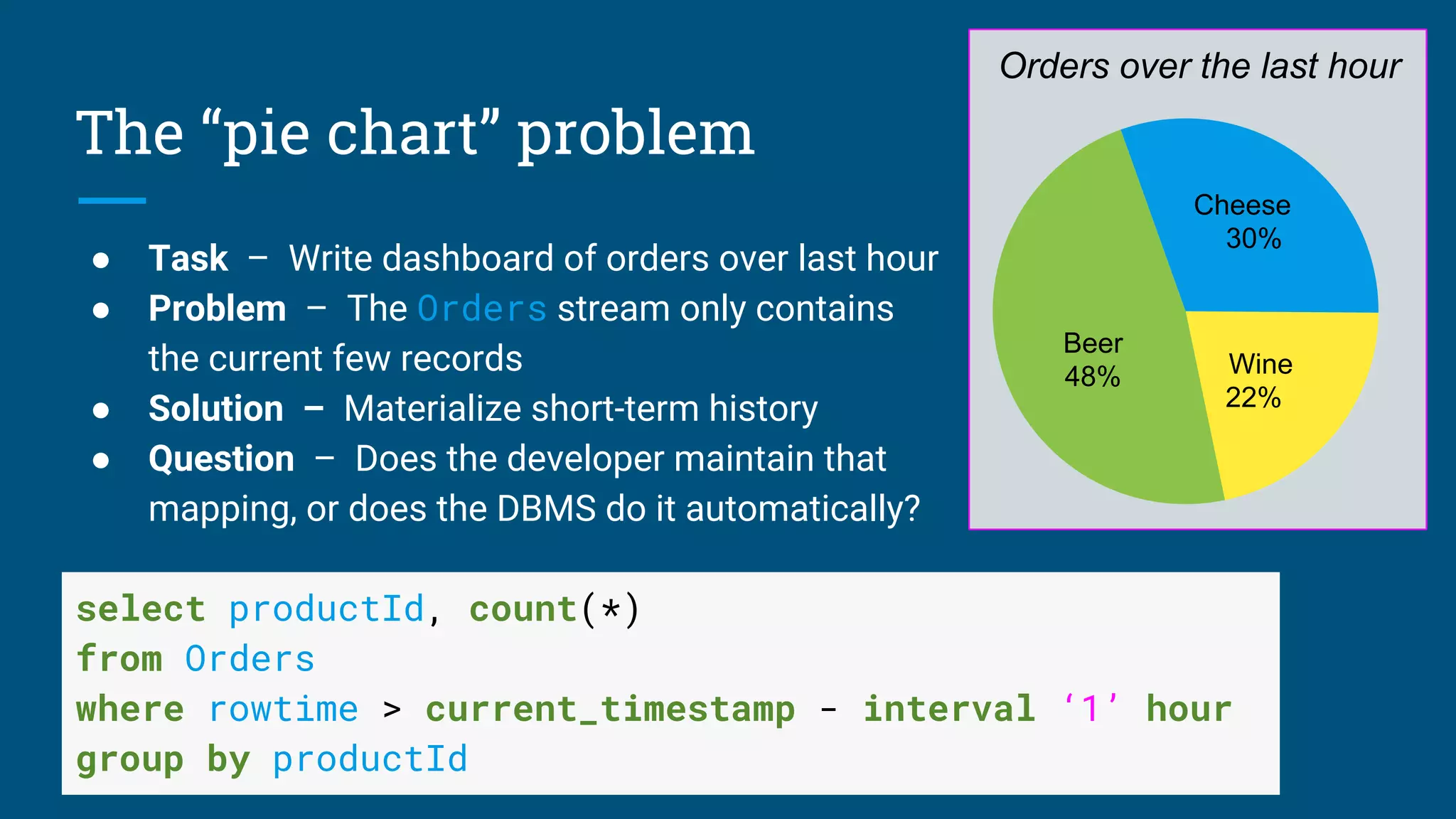
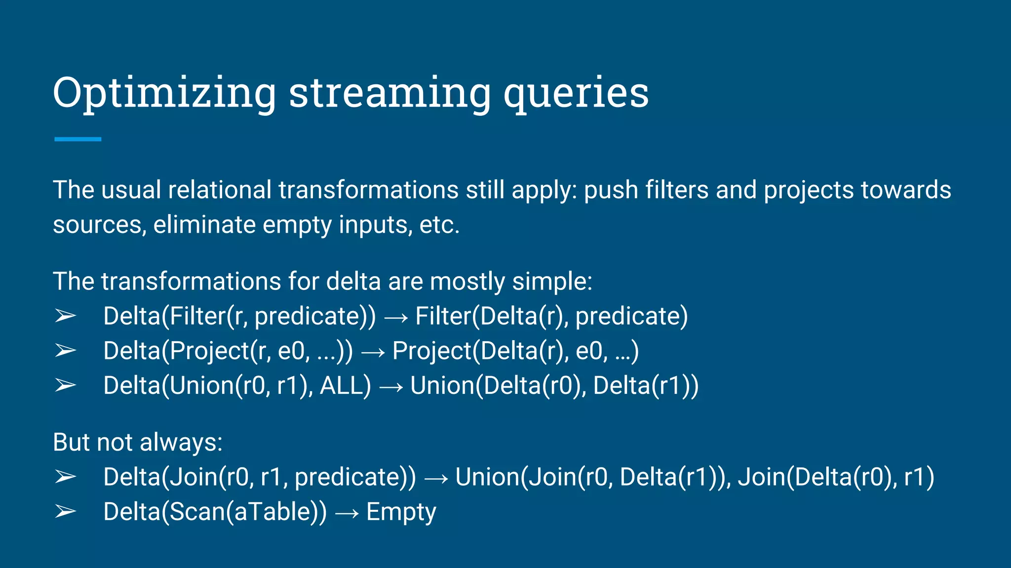
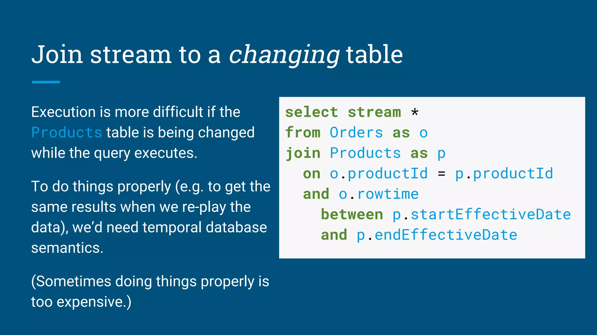
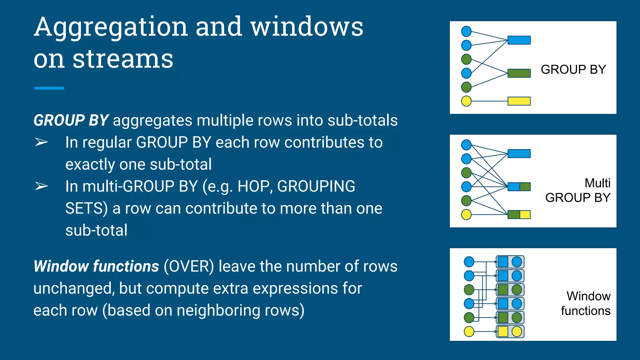
Techniques for optimizing streaming queries with different windowing strategies and handling data changes.


![[WSO2Con EU 2018] Streaming SQL in the Real World](https://cdn.slidesharecdn.com/ss_thumbnails/wso2coneu2018streamingsqlintherealworld-181113090808-thumbnail.jpg?width=640&height=640&fit=bounds)