Download as PDF, PPTX


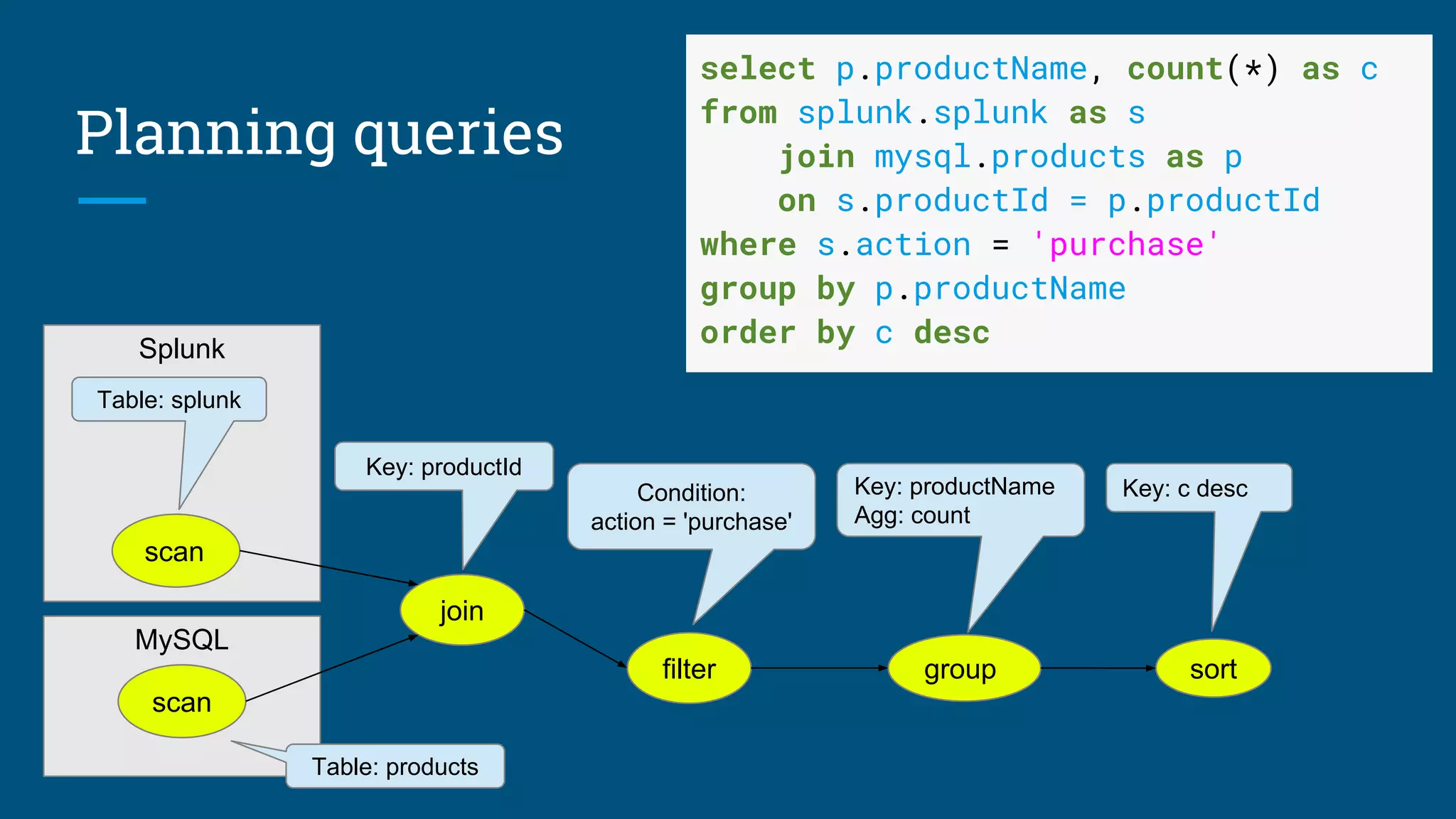
![Algorithm: Design summary tables
Given a database with 30 columns, 10M rows. Find X summary tables with under
Y rows that improve query response time the most.
AdaptiveMonteCarlo algorithm [1]:
● Based on research [2]
● Greedy algorithm that takes a combination of summary tables and tries to
find the table that yields the greatest cost/benefit improvement
● Models “benefit” of the table as query time saved over simulated query load
● The “cost” of a table is its size
[1] org.pentaho.aggdes.algorithm.impl.AdaptiveMonteCarloAlgorithm
[2] Harinarayan, Rajaraman, Ullman (1996). “Implementing data cubes efficiently”](https://image.slidesharecdn.com/calcite-profiling-summit-2017-170614175054/75/Data-profiling-with-Apache-Calcite-10-2048.jpg)
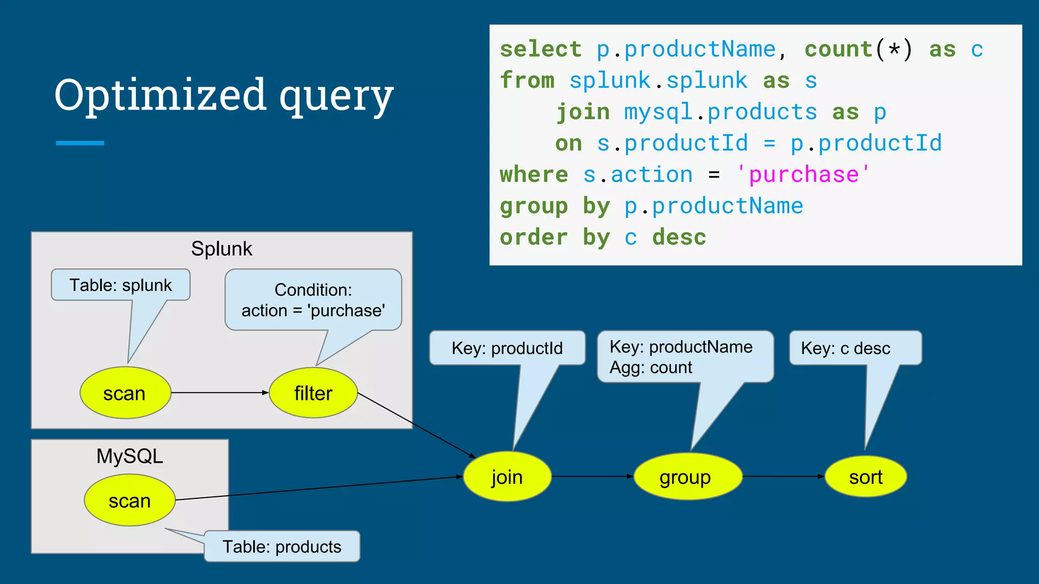
![Sketches
HyperLogLog is an algorithm that computes
approximate distinct count. It can estimate
cardinalities of 109
with a typical error rate of
2%, using 1.5 kB of memory. [3][4]
With 16 MB memory per machine we can
compute 10,000 combinations of attributes
each pass.
So, we’re down from 109
to 105
passes.
[3] Flajolet, Fusy, Gandouet, Meunier (2007). "Hyperloglog: The analysis of a near-optimal cardinality estimation algorithm"
[4] https://github.com/mrjgreen/HyperLogLog](https://image.slidesharecdn.com/calcite-profiling-summit-2017-170614175054/75/Data-profiling-with-Apache-Calcite-14-2048.jpg)


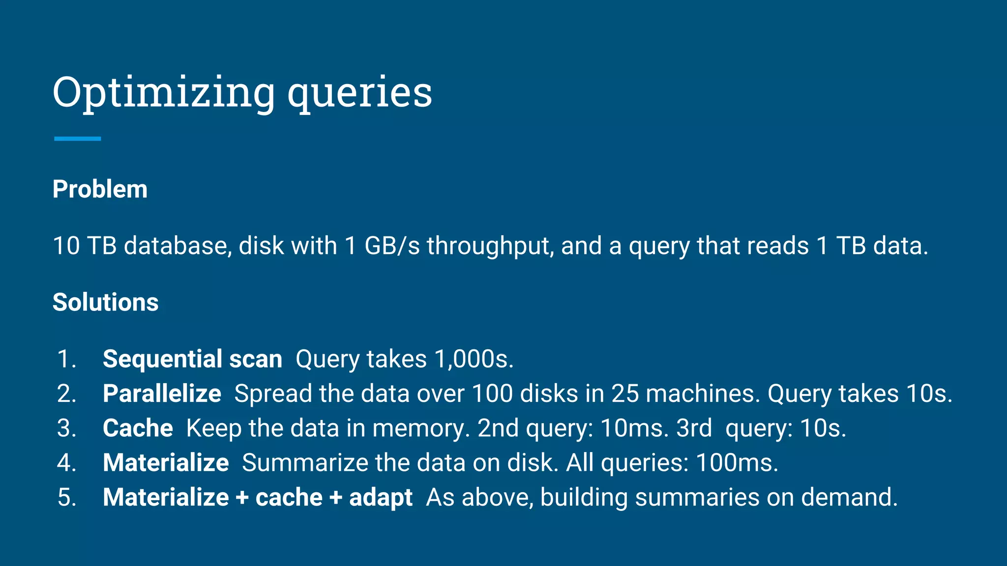
![Algorithm: Design summary tables
Given a database with 30 columns, 10M rows. Find X summary tables with under
Y rows that improve query response time the most.
AdaptiveMonteCarlo algorithm [1]:
● Based on research [2]
● Greedy algorithm that takes a combination of summary tables and tries to
find the table that yields the greatest cost/benefit improvement
● Models “benefit” of the table as query time saved over simulated query load
● The “cost” of a table is its size
[1] org.pentaho.aggdes.algorithm.impl.AdaptiveMonteCarloAlgorithm
[2] Harinarayan, Rajaraman, Ullman (1996). “Implementing data cubes efficiently”](https://crownmelresort.com/image.slidesharecdn.com/calcite-profiling-summit-2017-170614175054/75/Data-profiling-with-Apache-Calcite-10-2048.jpg)


![Sketches
HyperLogLog is an algorithm that computes
approximate distinct count. It can estimate
cardinalities of 109
with a typical error rate of
2%, using 1.5 kB of memory. [3][4]
With 16 MB memory per machine we can
compute 10,000 combinations of attributes
each pass.
So, we’re down from 109
to 105
passes.
[3] Flajolet, Fusy, Gandouet, Meunier (2007). "Hyperloglog: The analysis of a near-optimal cardinality estimation algorithm"
[4] https://github.com/mrjgreen/HyperLogLog](https://crownmelresort.com/image.slidesharecdn.com/calcite-profiling-summit-2017-170614175054/75/Data-profiling-with-Apache-Calcite-14-2048.jpg)


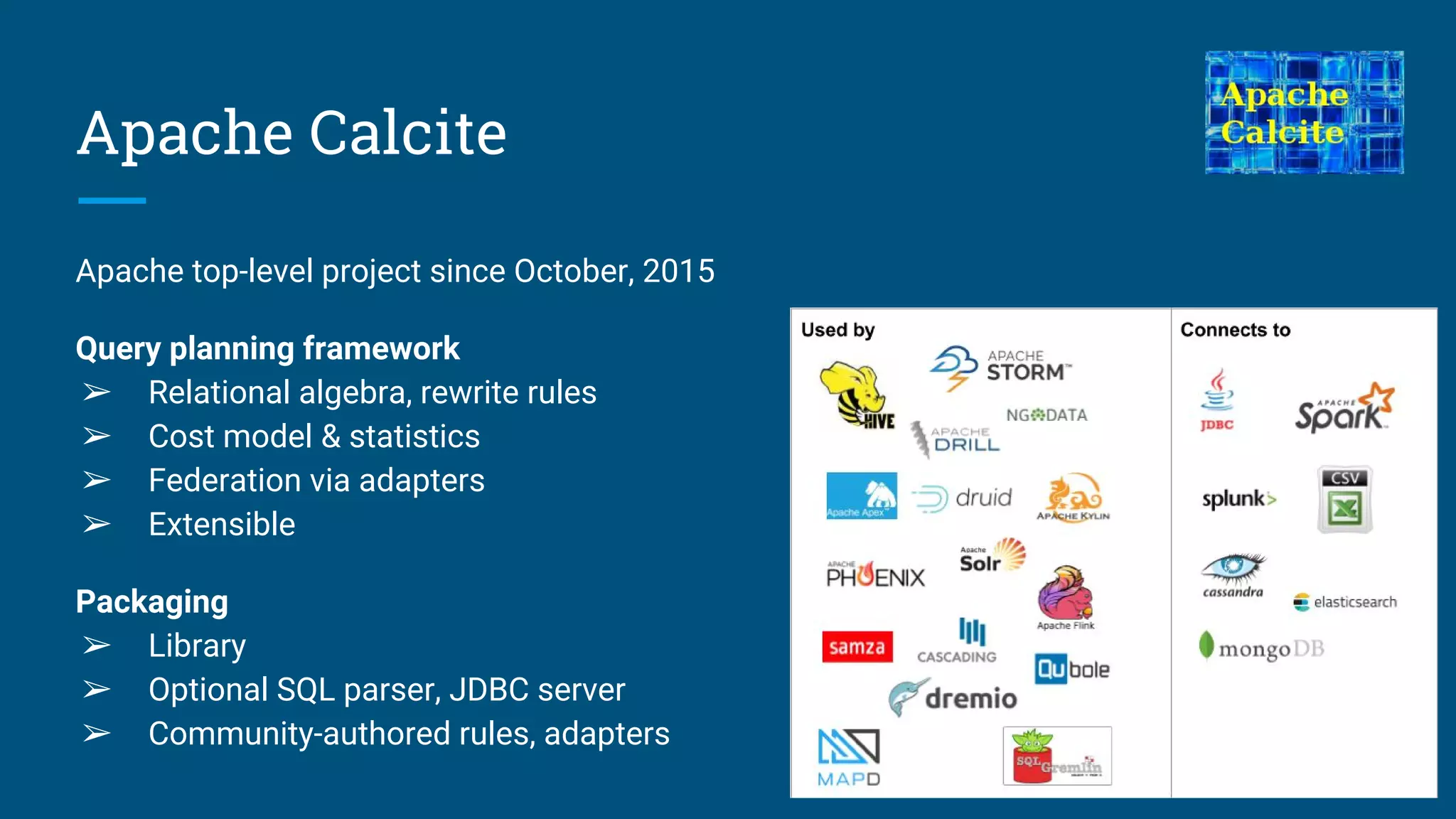
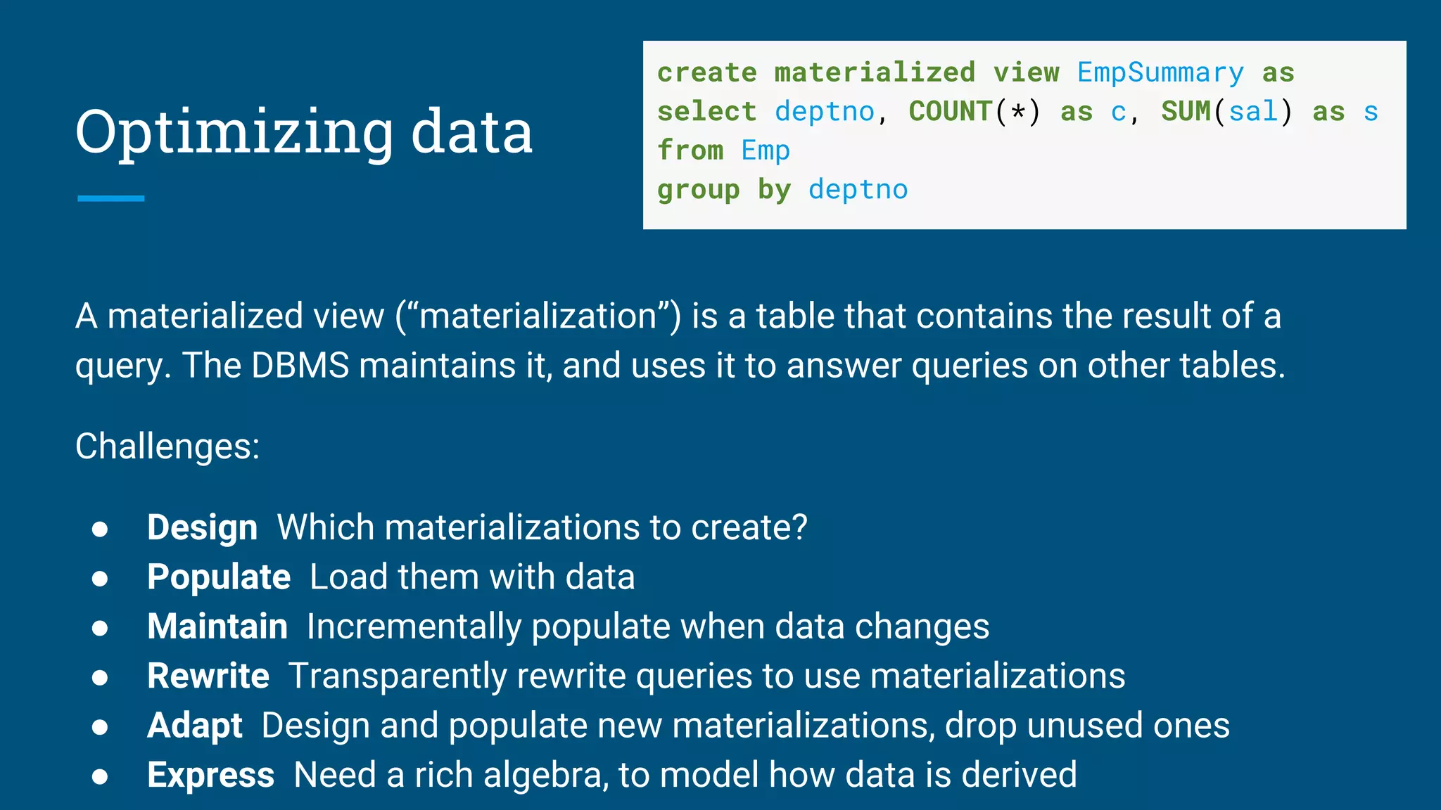
The document discusses data profiling using Apache Calcite, focusing on the design and optimization of summary tables and query performance improvement techniques. It covers algorithms for profiling data, including the Adaptive Monte Carlo algorithm, which helps determine the most efficient summary tables for improving query response times. The challenges of materialization and the application of sketches and parallelism in the profiling process are also highlighted.