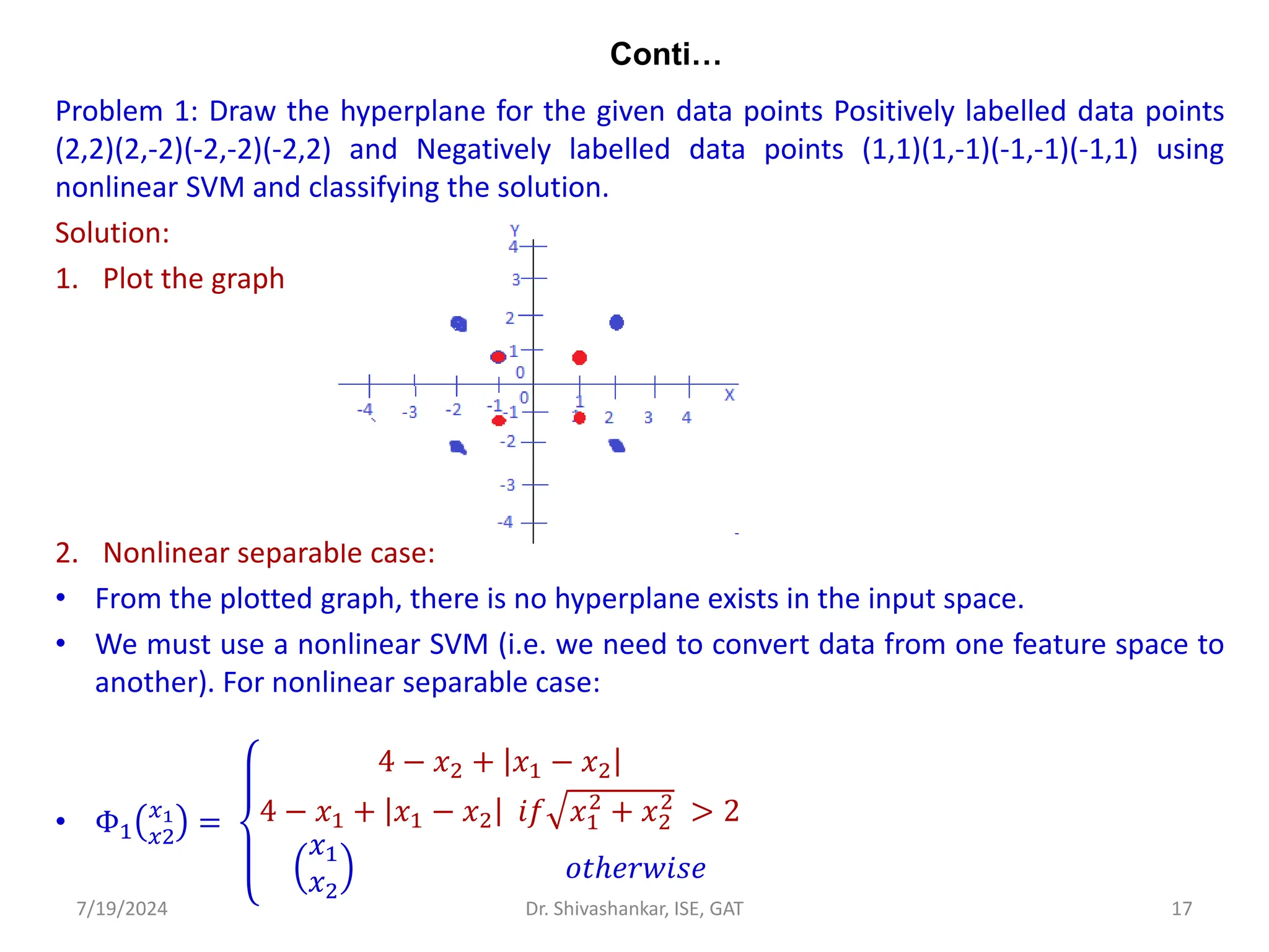
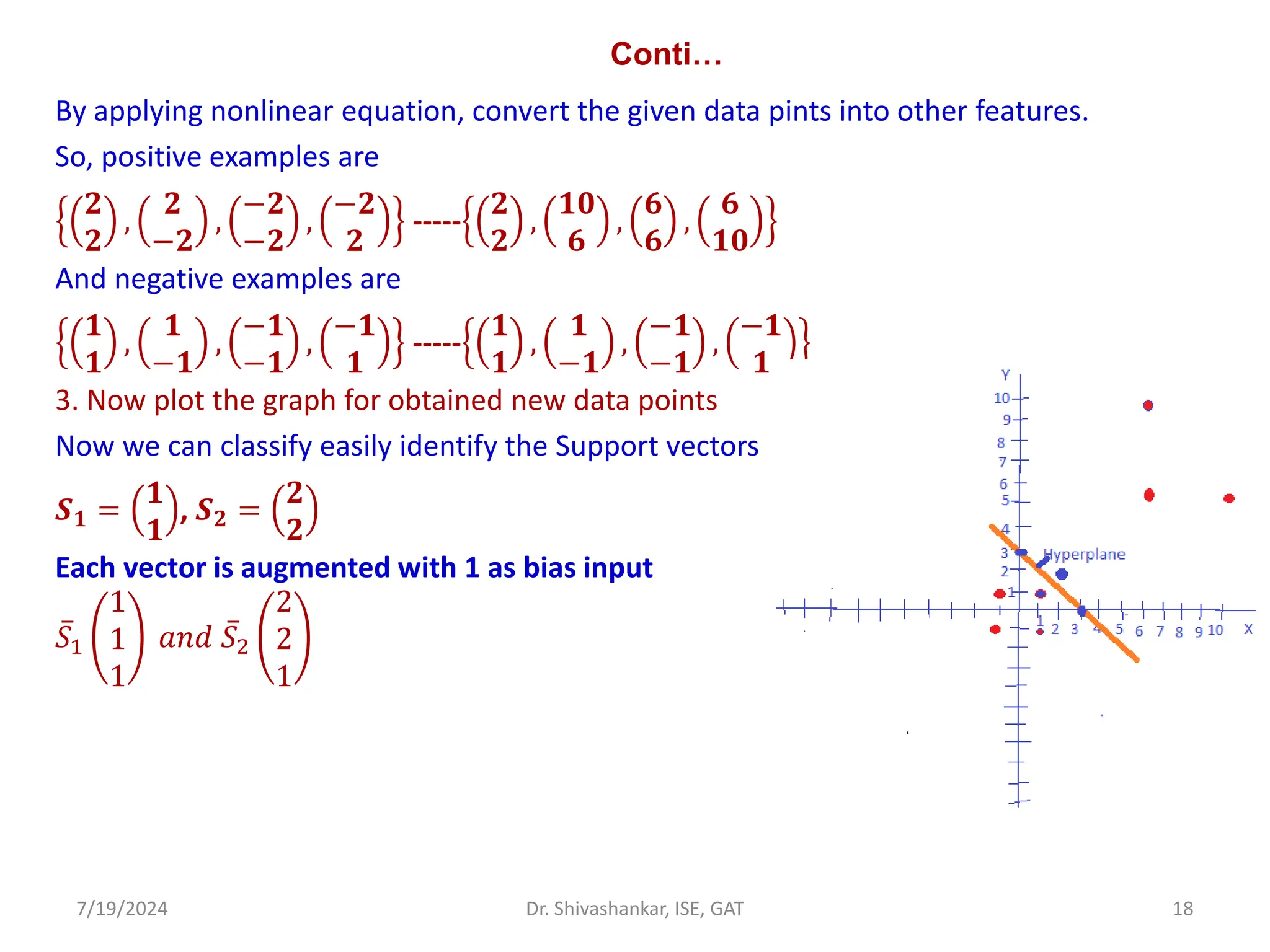
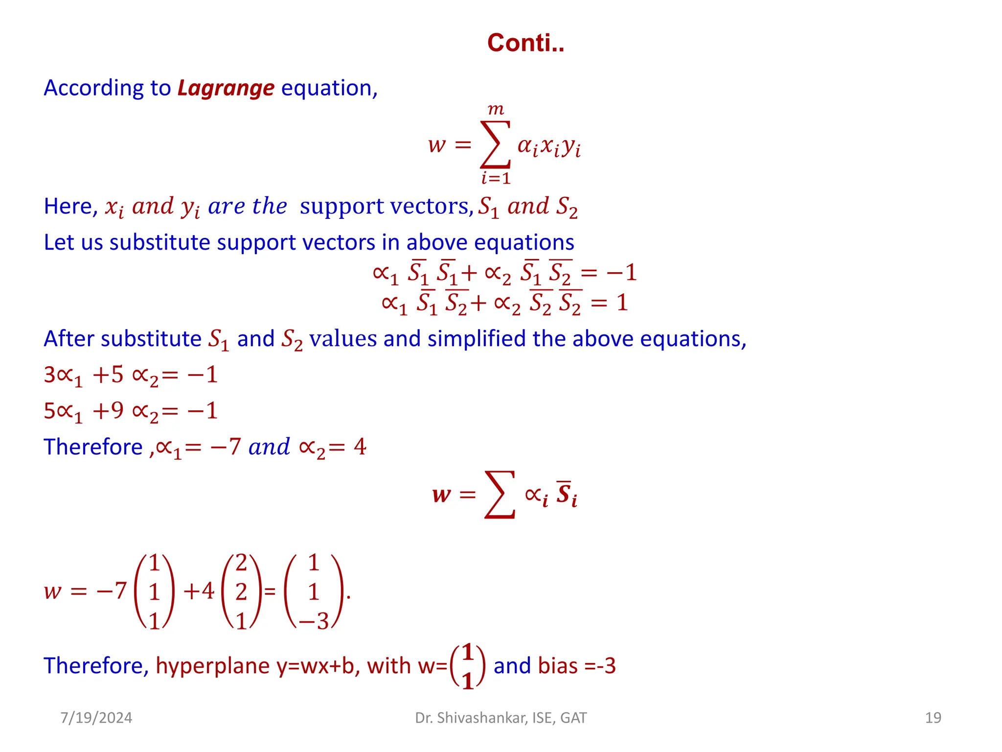
The document discusses Support Vector Machines (SVM), a supervised learning algorithm used for classification and regression. It covers the concept of hyperplanes, the importance of support vectors in finding optimal decision boundaries, and different types of SVMs, including linear and non-linear SVMs. Additionally, it explains various terminologies related to SVM, such as margin, kernels, and the hinge loss function.
![SVM Implementation in Python
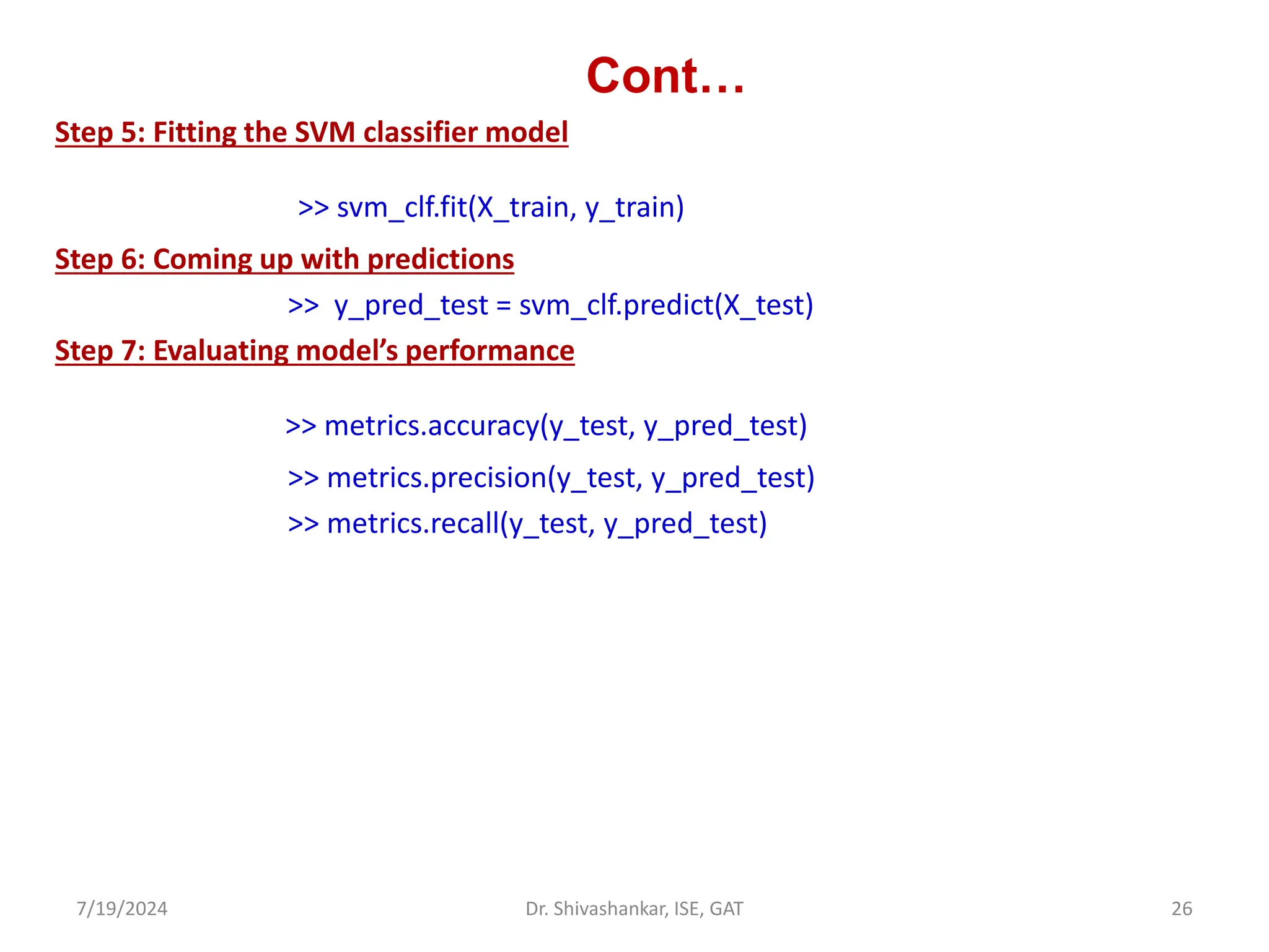
In Python, an SVM classifier can be developed using the sklearn library.
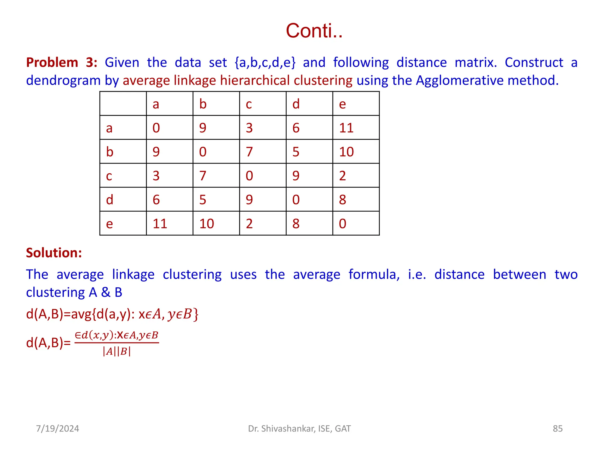
Step 1: Load the important libraries
>> import pandas as pd
>> import numpy as np
>> import sklearn
>> from sklearn import svm
>> from sklearn.model_selection import train_test_split
>> from sklearn import metrics
Step 2: Import dataset and extract the X variables and Y separately.
>> df = pd.read_csv(“mydataset.csv”)
>> X = df.loc[:,[‘Var_X1’,’Var_X2’,’Var_X3’,’Var_X4’]]
>> Y = df[[‘Var_Y’]]
Step 3: Divide the dataset into train and test
>> X_train, X_test, y_train, y_test = train_test_split(X, Y, test_size = 0.3,
random_state=123)
Step 4: Initializing the SVM classifier mode
>> svm_clf = svm.SVC(kernel = ‘linear’)
7/19/2024 25
Dr. Shivashankar, ISE, GAT](https://image.slidesharecdn.com/machinelearning-module2-240719092301-aa976ed7/75/Machine-Learning_SVM_KNN_K-MEANSModule-2-pdf-25-2048.jpg)
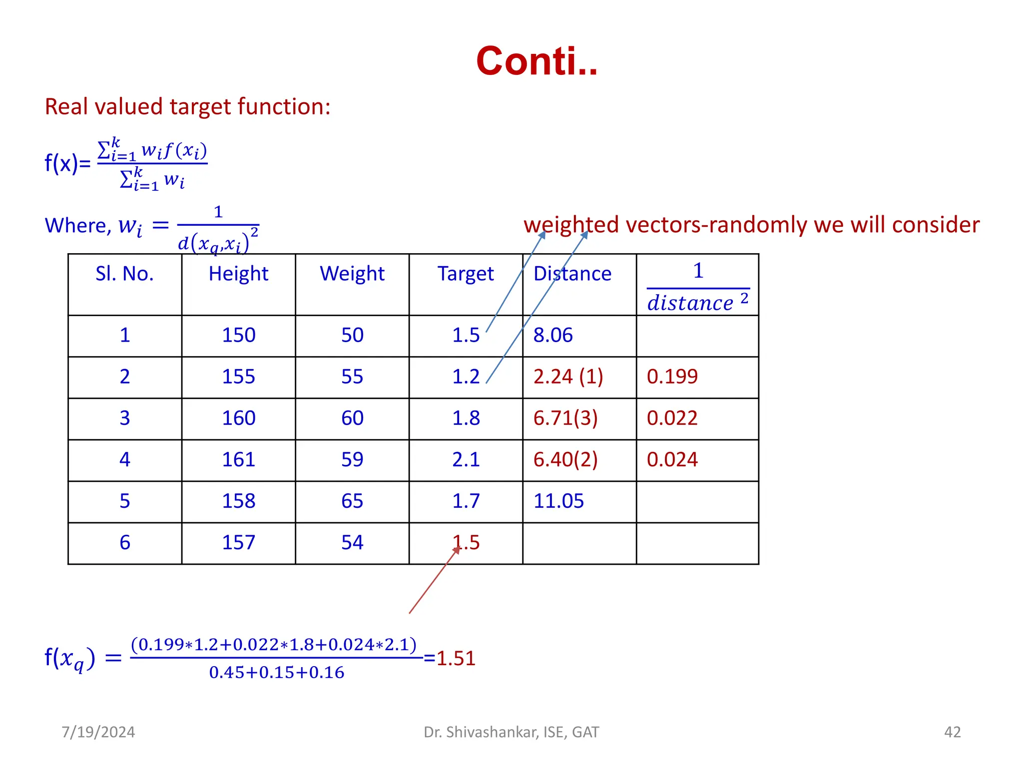
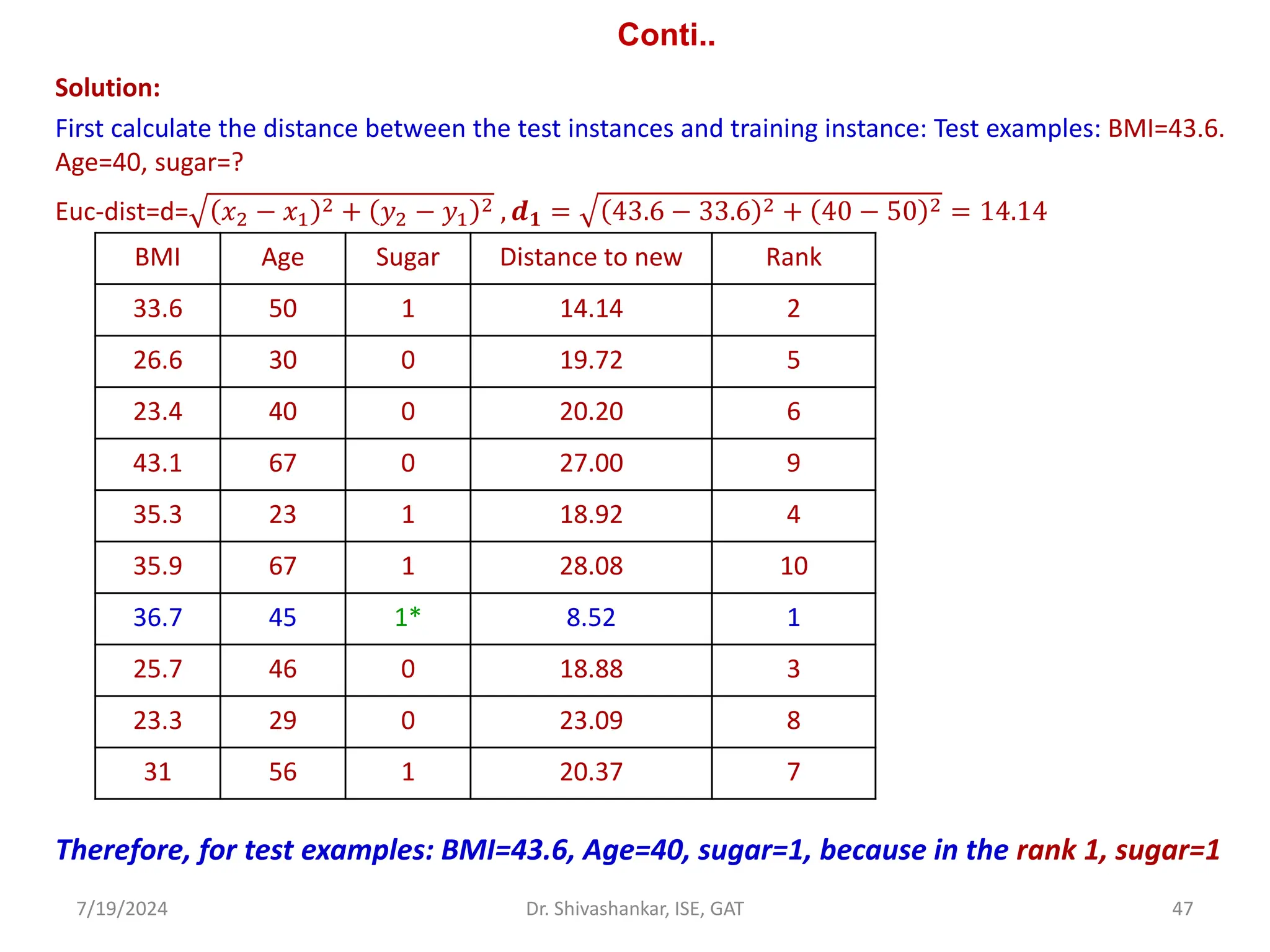
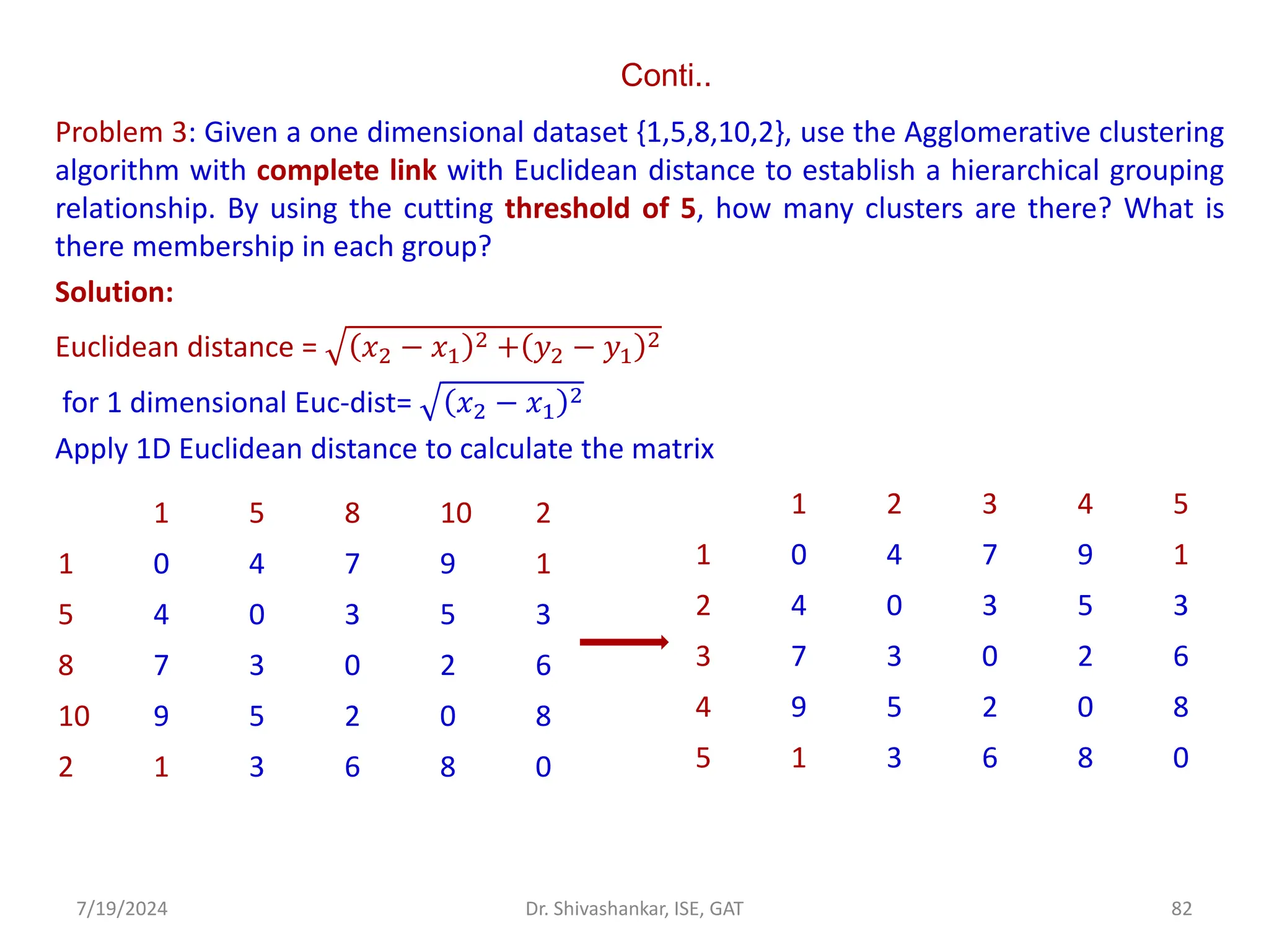
![Conti..
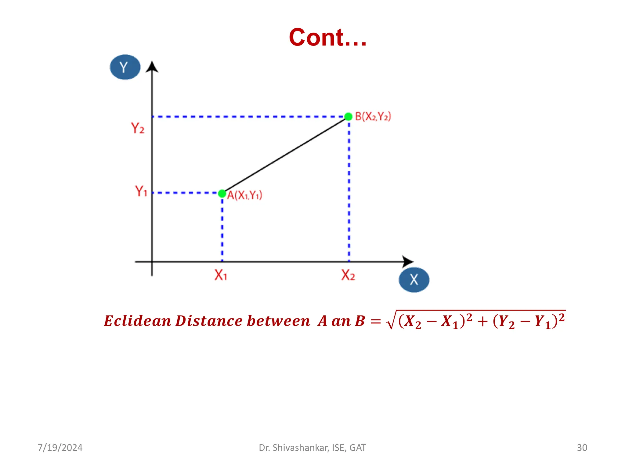
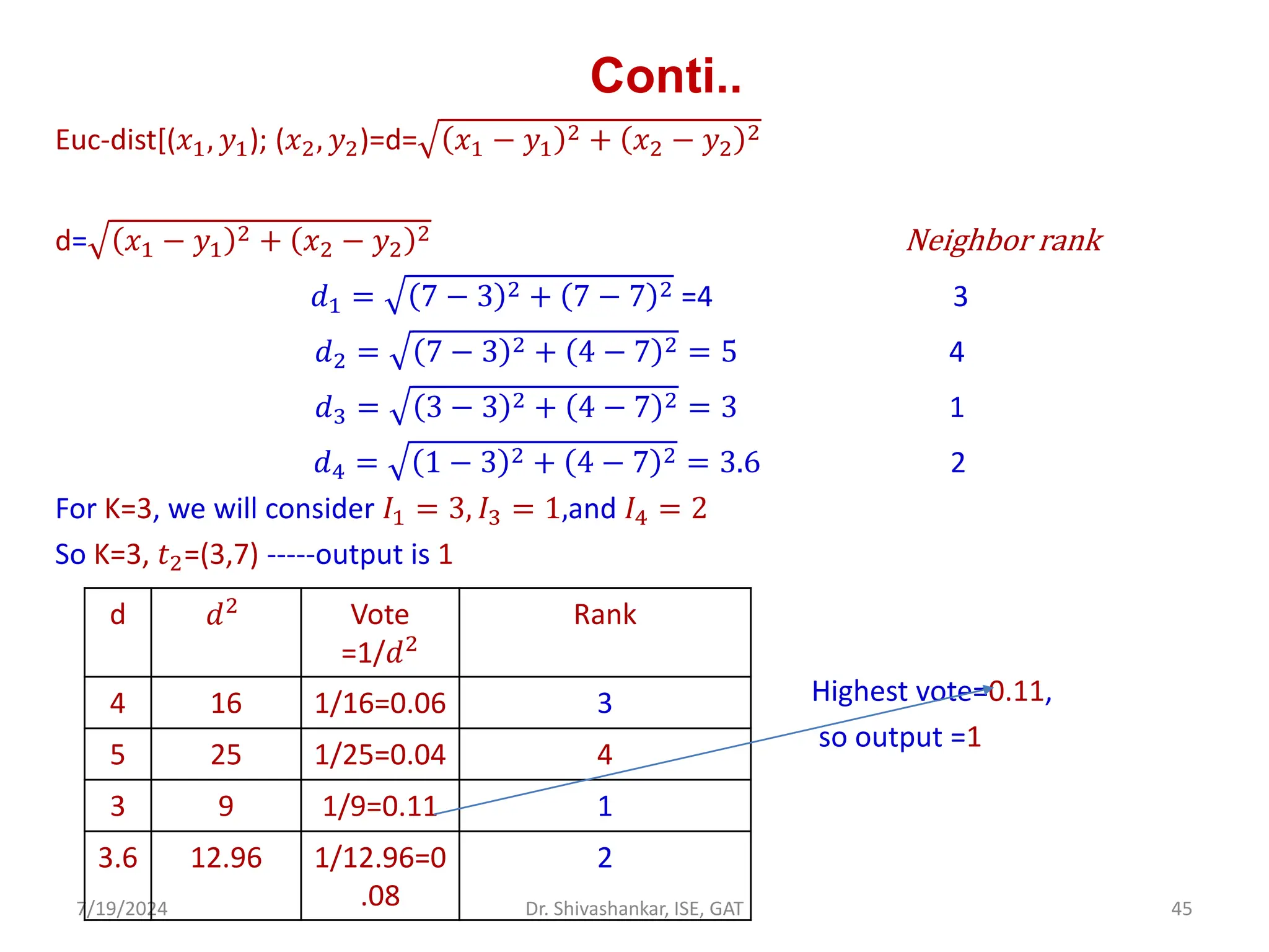
Euc-dist[(𝑥1, 𝑦1); (𝑥2, 𝑦2)= 𝑥2 − 𝑥1
2 + 𝑦2 − 𝑦1
2
Class A : [(6,5);(4,2)] = 4 − 6 2 + 2 − 5 2 = 3.6
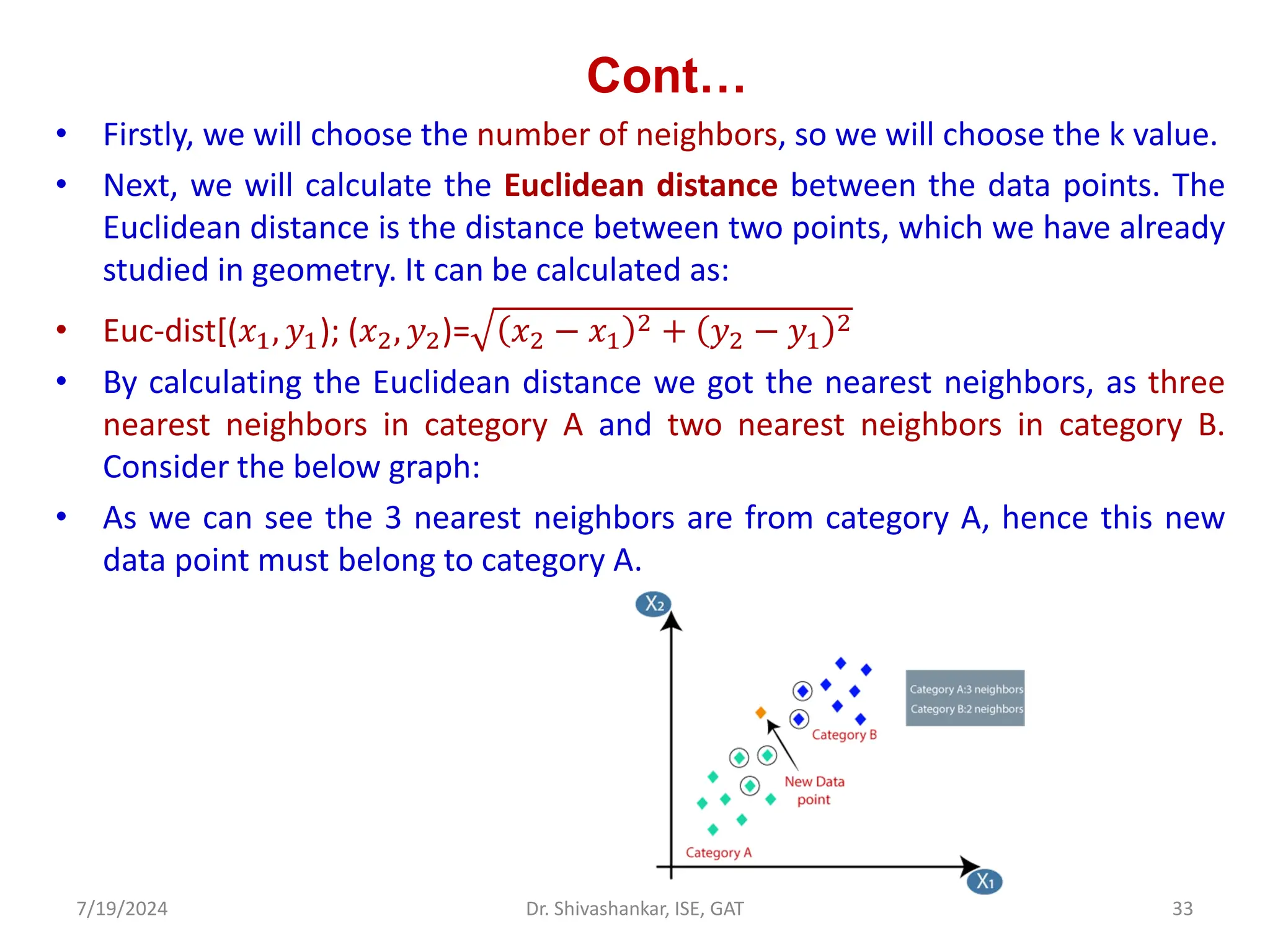
Class B: [(6,5);(7,6)] = 7 − 6 2 + 6 − 5 2 =1.414
The test instance has smaller distance to class B
Hence, the class of this test instance is predicted as B.
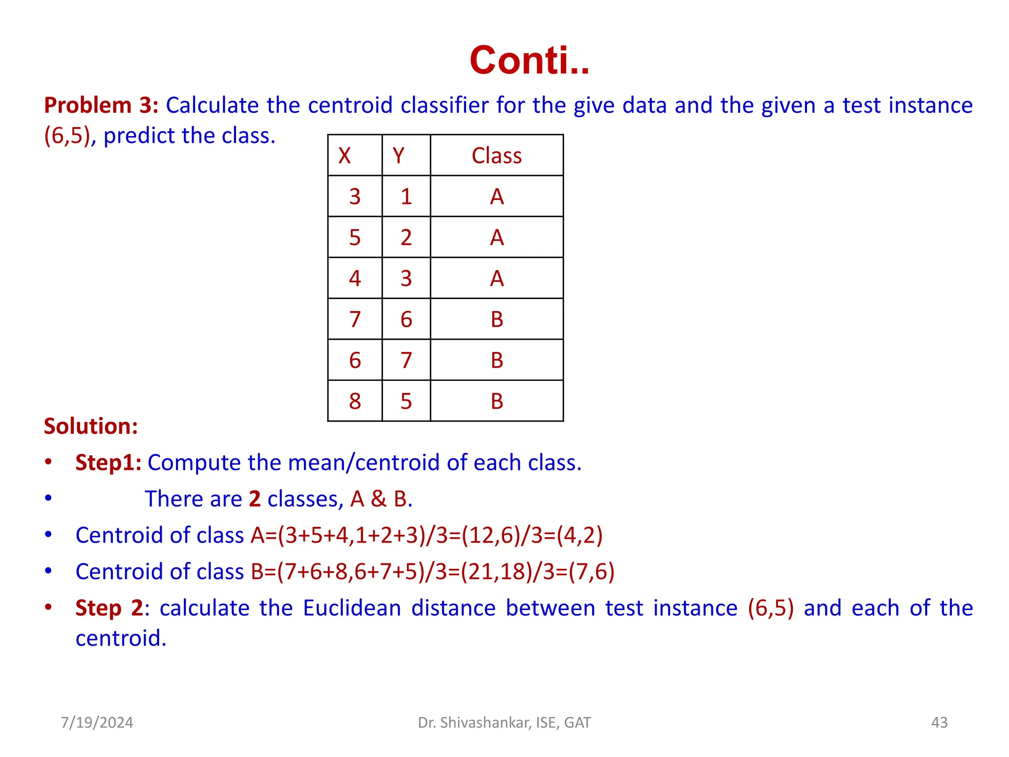
Problem 4. Given the following training instances in the table, each having two attributes
(x1 and x2). Compute the class label for test instance 𝑡1 = 3,7 , using 3 nearest neighbors
(k=3).
7/19/2024 44
Dr. Shivashankar, ISE, GAT
Training
Instances
𝑥1 𝑥2 Output
𝐼1 7 7 0
𝐼2 7 4 0
𝐼3 3 4 1
𝐼4 1 4 1](https://image.slidesharecdn.com/machinelearning-module2-240719092301-aa976ed7/75/Machine-Learning_SVM_KNN_K-MEANSModule-2-pdf-44-2048.jpg)
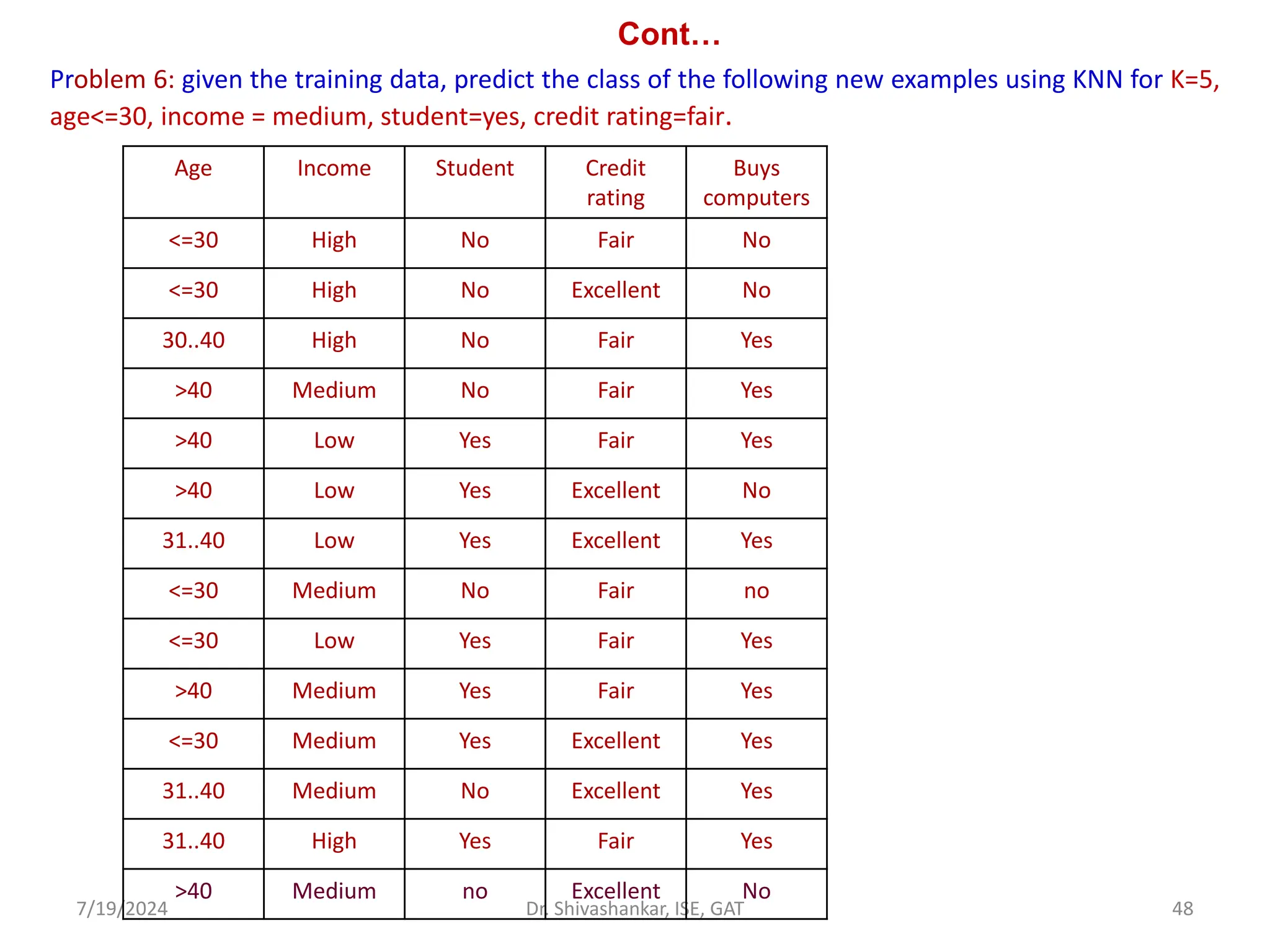
![Cont…
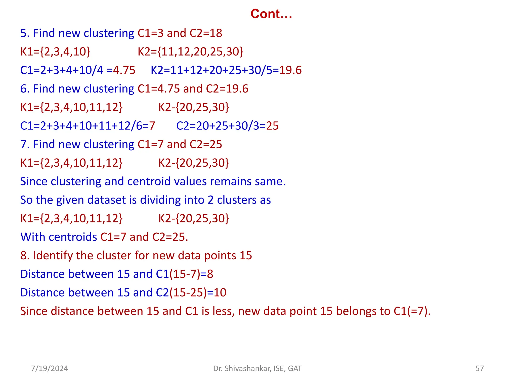
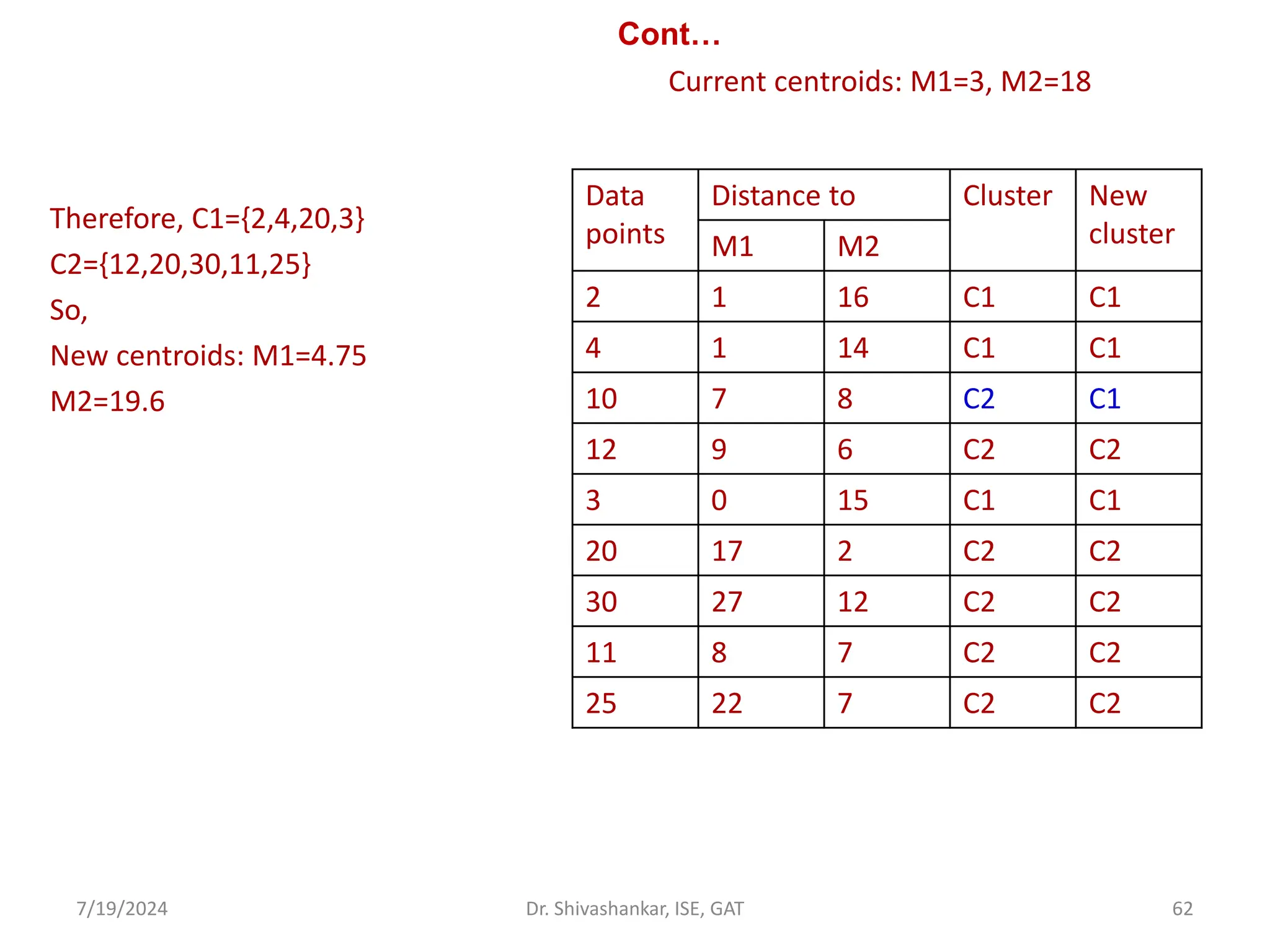
Problem 1: Divide the given sample data into two clusters [2] using K means algorithm
S={2,3,4,10,11,12,20,25,30}. Given K=2, for new data point 15, identify the cluster belongs
to.
Solution:
1. Choose 2 random clusters from the given data sets C1=4, C2=12.
2. Find the distance between given samples and centroids, put the sample in the nearest
cluster.
3. Repeat the same for all data points.
Cluster k1={2,3,4} -------------(2-4=2, 3-4=1, 4-4=0, 10-4=6,……..
2-12=10, 3-12=9, 5-12=7, 10-12=2,……..
so 2,3 and 4 are placed in cluster 1 as its distance is nearest
to C1=4 and
Cluster K2={10,11,12,20,25,30}
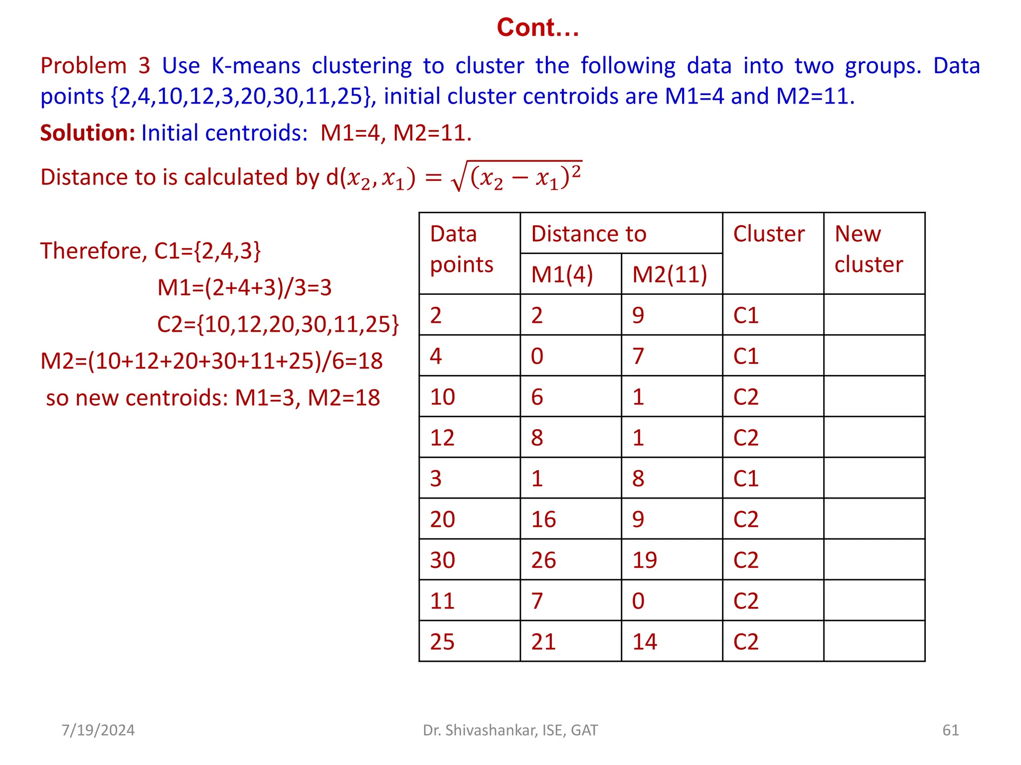
4. Compute new centroids
K1={2,3,4} K2={10,11,12,20,25,30}
C1={2+3+4/3}=3 C2={10+11+12+20+25+30}/6=18
So C1=3 C2=18
7/19/2024 56
Dr. Shivashankar, ISE, GAT](https://image.slidesharecdn.com/machinelearning-module2-240719092301-aa976ed7/75/Machine-Learning_SVM_KNN_K-MEANSModule-2-pdf-56-2048.jpg)
![Cont…
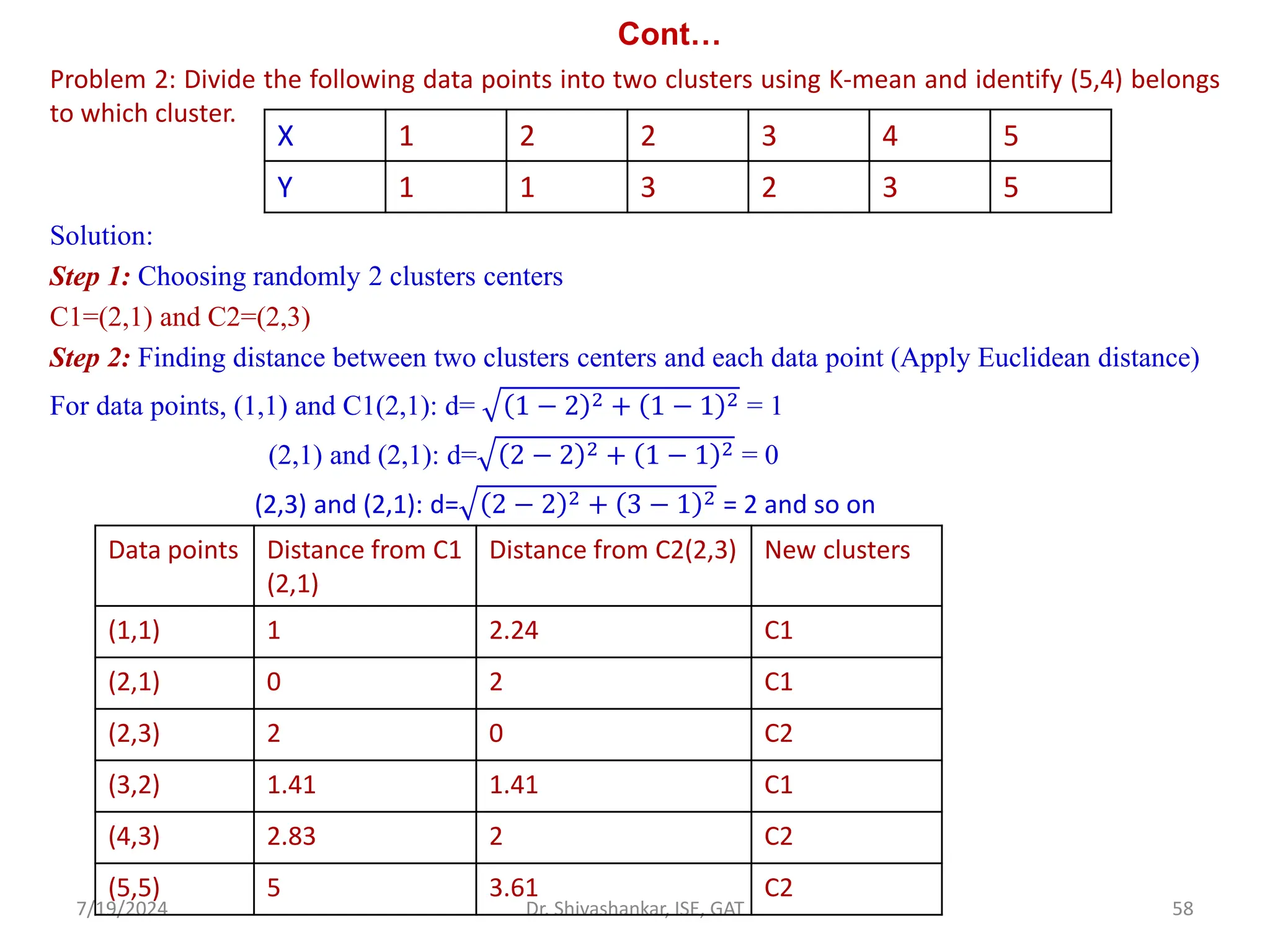
Step 3: cluster 1 of C1={ (1,1), (2,1), (3,2)}
cluster 2 of C2={ (2,3), (4,3), (5,5)}
Step 4: Recalculate cluster center
C1=
1
3
[(1,1)+(2,1)+(3,2)]=
1
3
[6,4]= (2,1.33)
C2=
1
3
[(2,3)+(4,3)+(5,5)]=
1
3
[11,11]= (3.67,3.67)
Step 5: Repeat the step 2 until we get same cluster center or same cluster elements
7/19/2024 59
Dr. Shivashankar, ISE, GAT
Data points Distance from
C1(2,1.33)
Distance from
C2(3.67,3.67)
New clusters
(1,1) 1.05 3.78 C1
(2,1) 0.33 3.15 C1
(2,3) 1.67 1.8 C1
(3,2) 1.204 1.8 C1
(4,3) 2.605 0.75 C2
(5,5) 4.74 1.88 C2](https://image.slidesharecdn.com/machinelearning-module2-240719092301-aa976ed7/75/Machine-Learning_SVM_KNN_K-MEANSModule-2-pdf-59-2048.jpg)
![Cont…
cluster 1 of C1={ (1,1), (2,1),(2,3), (3,2)}
cluster 2 of C2={ (4,3), (5,5)}
Step 6: Recalculate cluster center
C1=
1
4
[(1,1)+(2,1)+(2,3)+(3,2)]=
1
4
[8,7]= (2,1.75)
C2=
1
2
[(4,3)+(5,5)]=
1
2
[9,8]= (4.5,4)
Step 7: Repeat the step 2 until we get same cluster center or same cluster elements
Step 8: cluster 1 of C1={ (1,1), (2,1),(2,3), (3,2)}
cluster 2 of C2={ (4,3), (5,5)}
Since cluster elements are same as compared to previous iteration, stop.
7/19/2024 60
Dr. Shivashankar, ISE, GAT
Data points Distance from C1(2,1.75) Distance from C2(4.5,4) New clusters
(1,1) 1.25 4.61 C1
(2,1) 0.75 3.9 C1
(2,3) 1.25 2.69 C1
(3,2) 1.03 2.5 C1
(4,3) 2.36 1.12 C2
(5,5) 4.42 1.12 C2](https://image.slidesharecdn.com/machinelearning-module2-240719092301-aa976ed7/75/Machine-Learning_SVM_KNN_K-MEANSModule-2-pdf-60-2048.jpg)
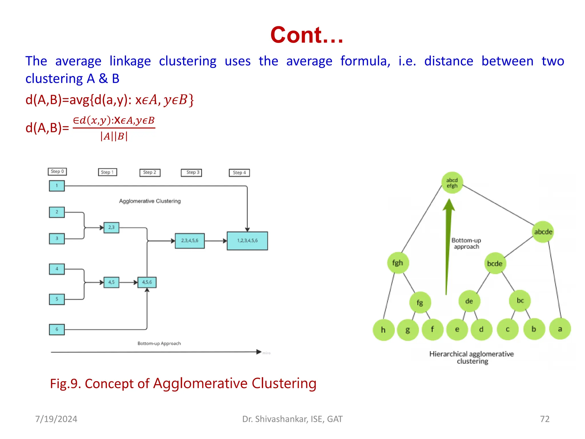
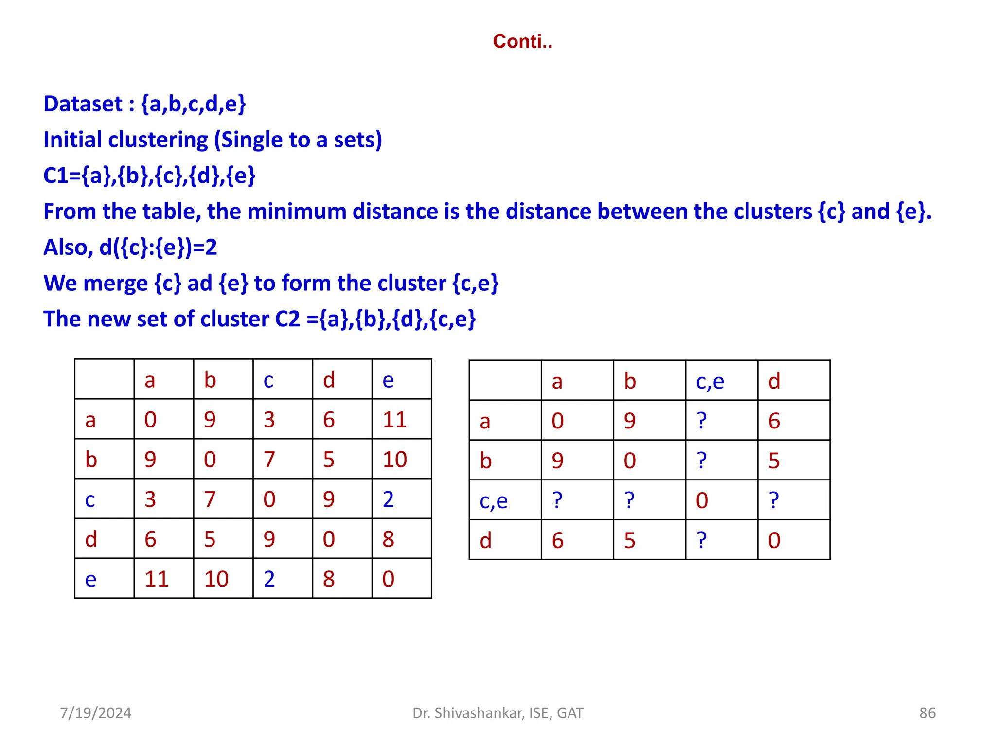
![Agglomerative Hierarchical Clustering Algorithm
• Step 1: Consider each dataset as a single cluster and calculate the distance of
one cluster from all the other clusters.
• Step 2: In the second step, comparable clusters are merged together to form
a single cluster. Let’s say cluster (B) and cluster (C) are very similar to each
other, therefore we merge them in the second step similarly to cluster (D)
and (E) and at last, we get the clusters [(A), (BC), (DE), (F)]
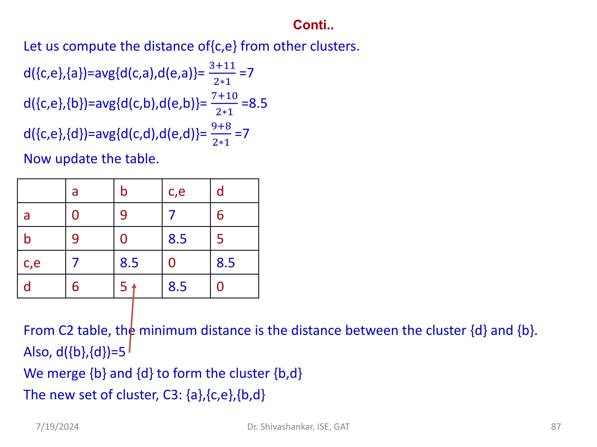
• Step 3: We recalculate the proximity according to the algorithm and merge
the two nearest clusters([(DE), (F)]) together to form new clusters as [(A),
(BC), (DEF)]
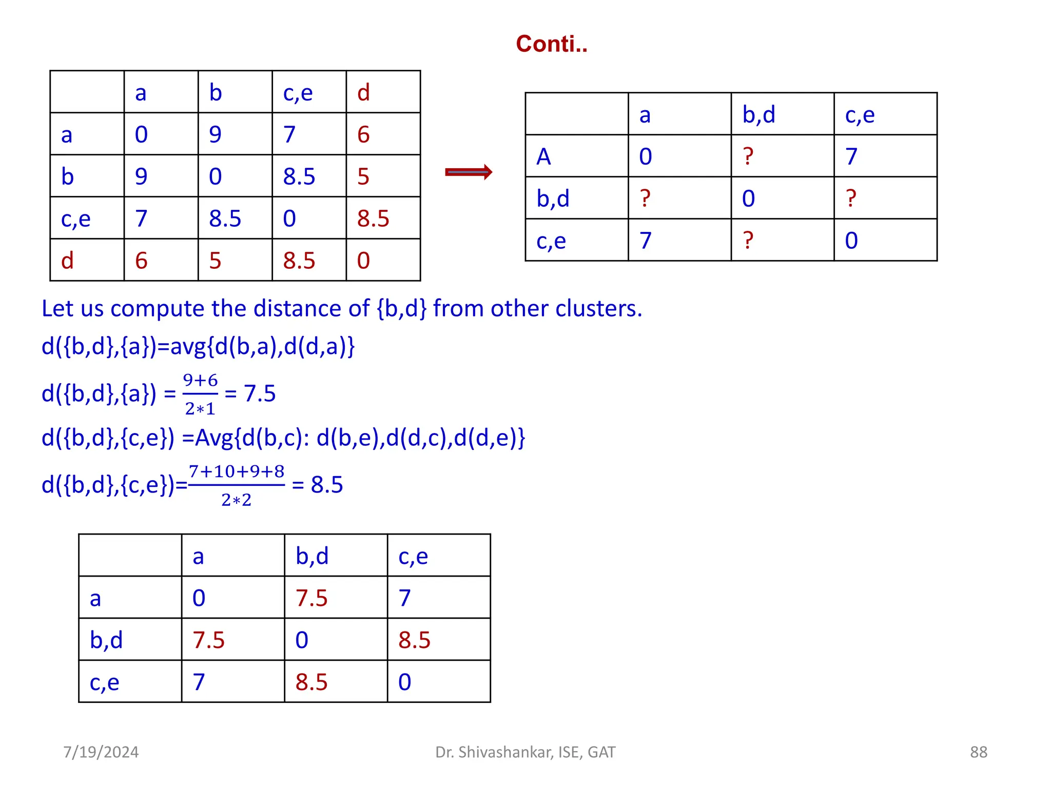
• Step 4: Repeating the same process; The clusters DEF and BC are comparable
and merged together to form a new cluster. We’re now left with clusters [(A),
(BCDEF)].
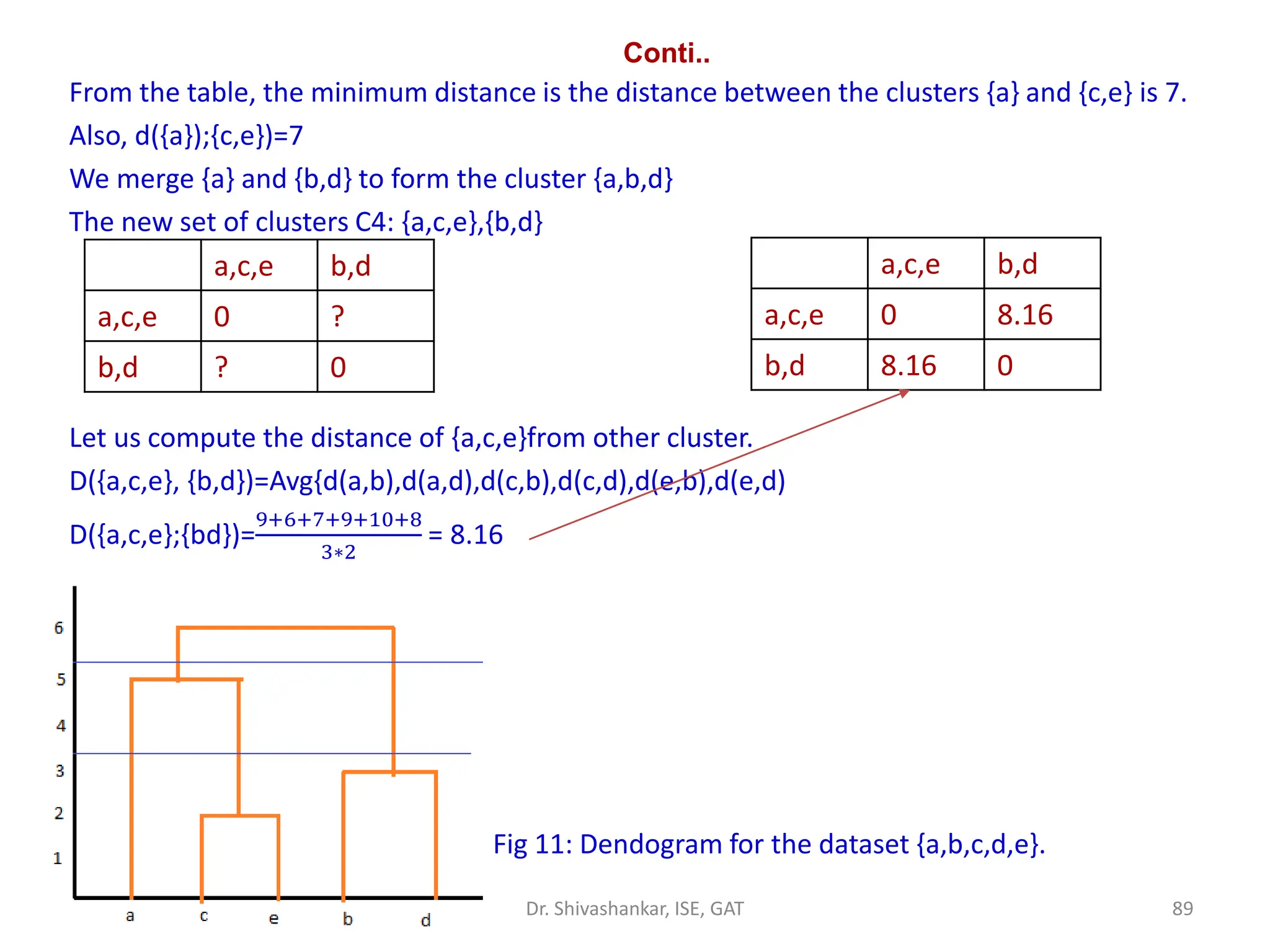
• Step 4: At last, the two remaining clusters are merged together to form a
single cluster [(ABCDEF)].
7/19/2024 71
Dr. Shivashankar, ISE, GAT](https://image.slidesharecdn.com/machinelearning-module2-240719092301-aa976ed7/75/Machine-Learning_SVM_KNN_K-MEANSModule-2-pdf-71-2048.jpg)
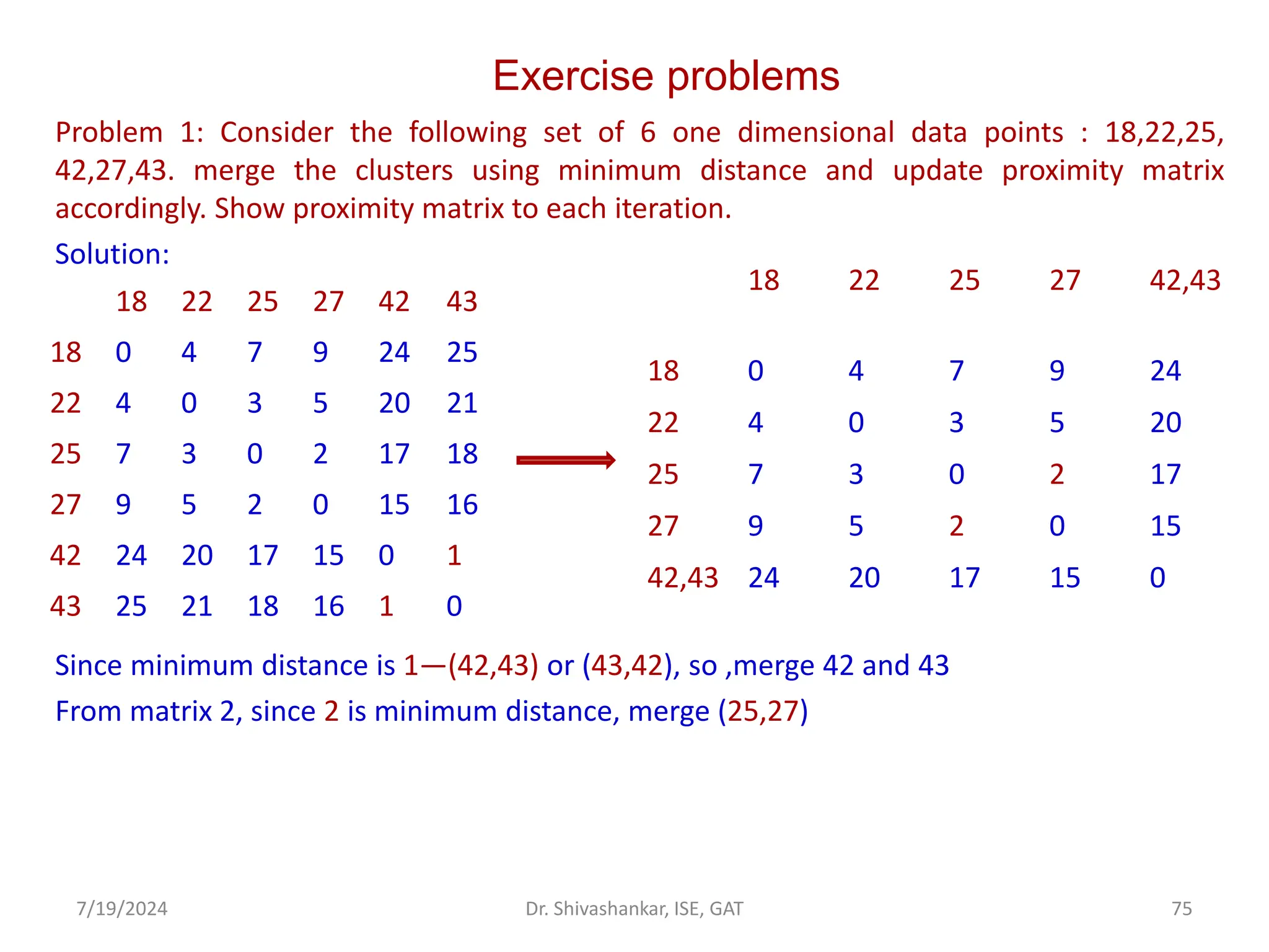
![Exercise problems
Since 3 is minimum distance, merge 22,25.and 27---{22,(25,27)}
Since 4 is minimum distance, merge 18,22,25,27---[18,{22,(25,27)}]
Draw the dendrogram for the merged data points.
7/19/2024 76
Dr. Shivashankar, ISE, GAT
18 22 25,27 42,43
18 0 4 7 24
22 4 0 3 20
25,27 7 3 0 15
42,43 24 20 15 0
18 22,25,27 42,43
18 0 4 24
22,25,27 4 0 15
42,43 24 15 0](https://image.slidesharecdn.com/machinelearning-module2-240719092301-aa976ed7/75/Machine-Learning_SVM_KNN_K-MEANSModule-2-pdf-76-2048.jpg)
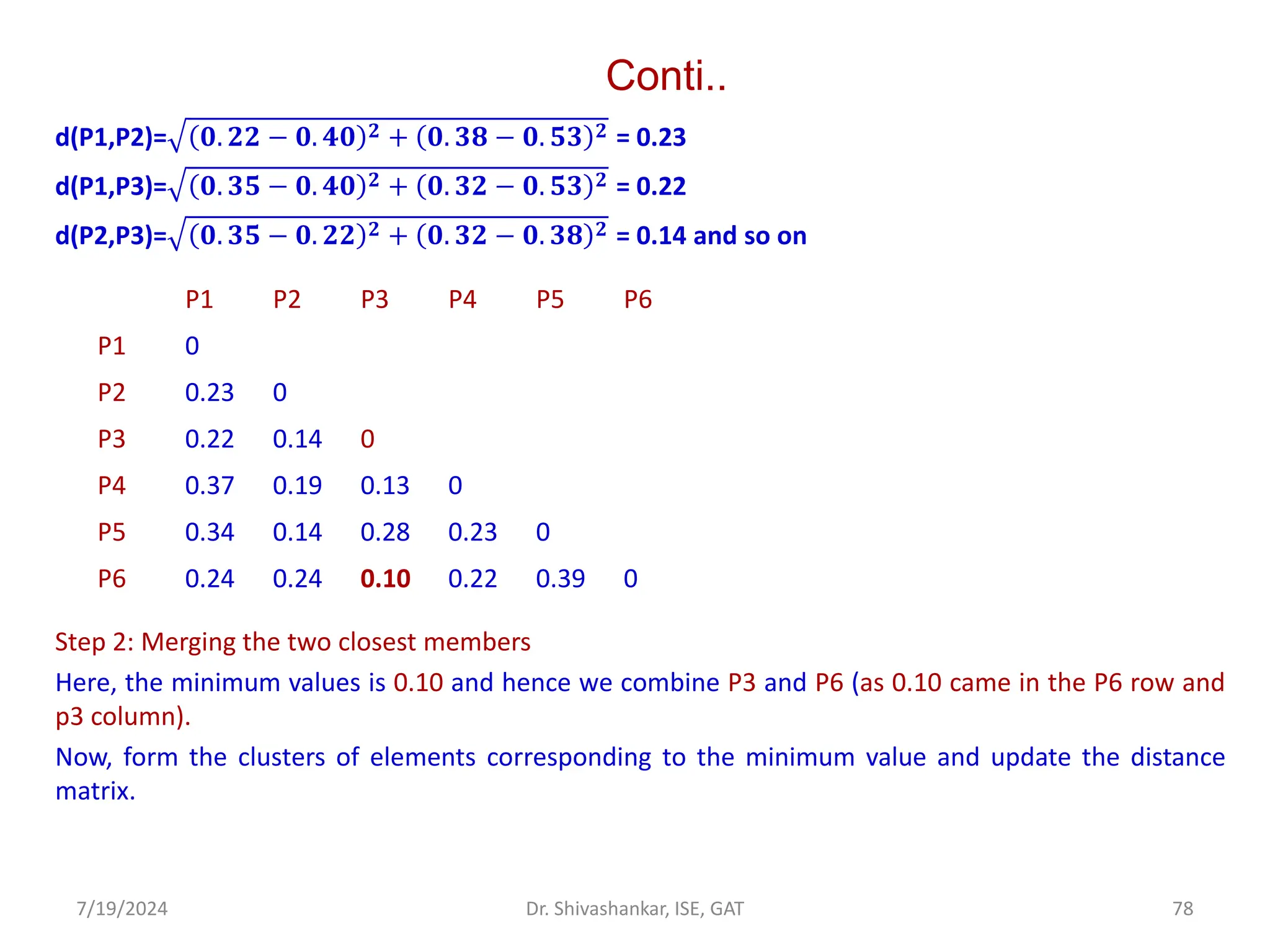
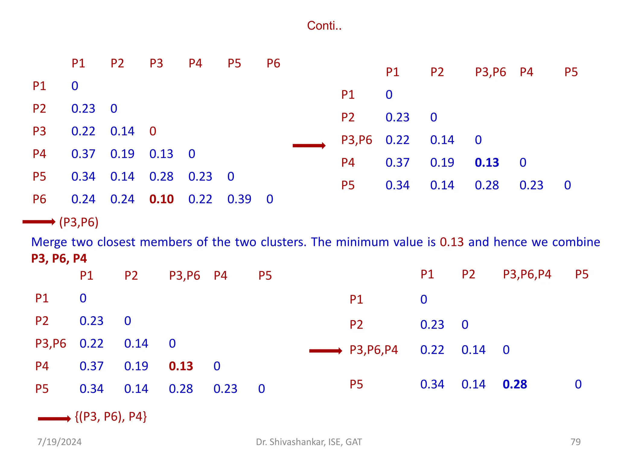
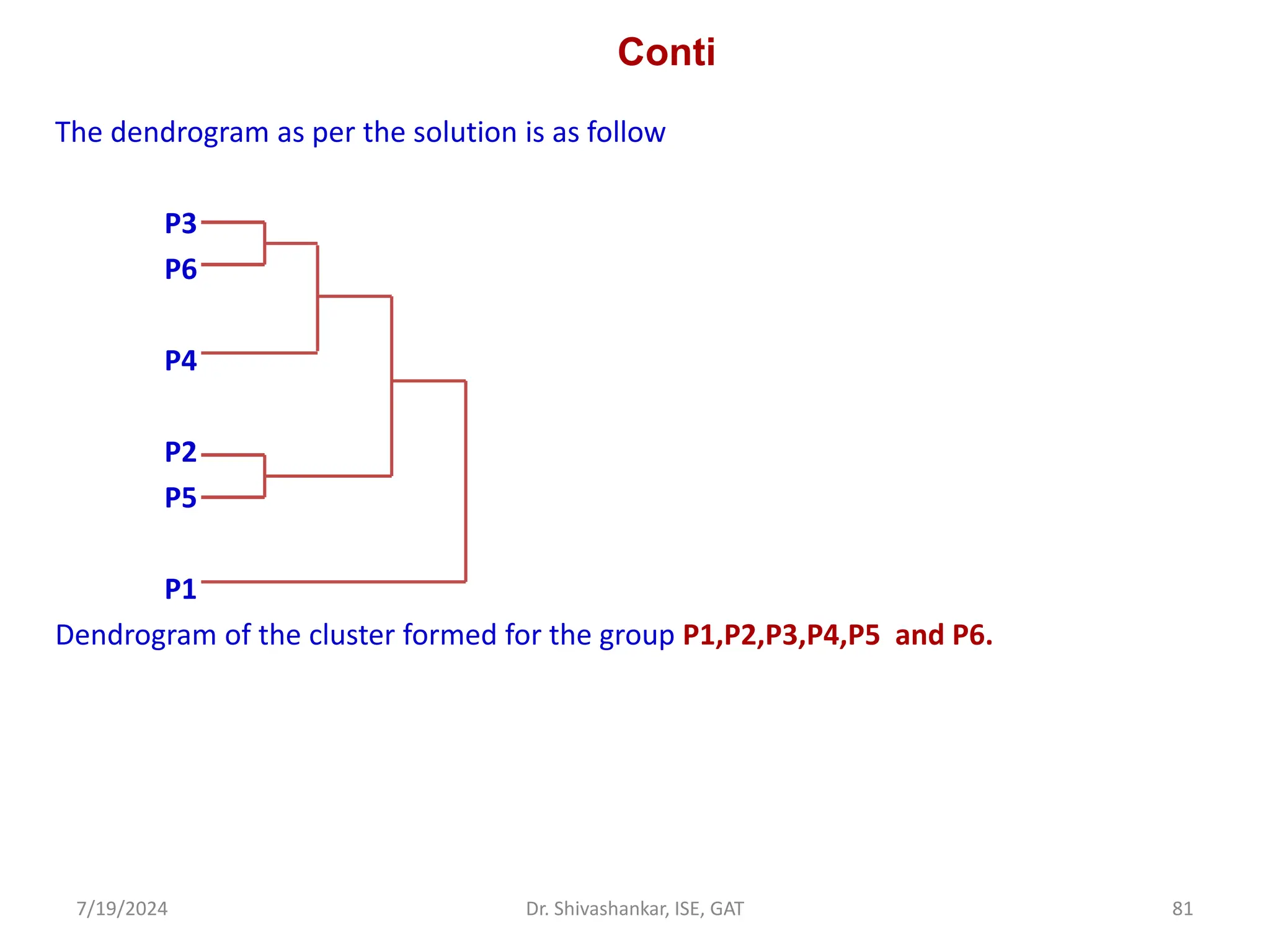
![Conti..
Now combined P2 and P5
[{(P3, P6), P4},(P2,P5)]
Now update the matrix and merge P2,P5,P3,P6 and P4
([{(P3, P6), P4},(P2,P5)], P1)
Now we have reached to the solution.
7/19/2024 80
Dr. Shivashankar, ISE, GAT
P1 P2 P3,P6,P4 P5
P1 0
P2 0.23 0
P3,P6,P4 0.22 0.14 0
P5 0.34 0.14 0.28 0
P1 P2,P5 P3,P6,P4
P1 0
P2,P5 0.23 0
P3,P6,P4 0.22 0.14 0
P1 P2,P5 P3,P6,P4
P1 0
P2,P5 0.23 0
P3,P6,P4 0.22 0.14 0
P1 P2,P5,P3,P6,P
4
P1 0
P2,P5,P3,P6,P4 0.22 0](https://image.slidesharecdn.com/machinelearning-module2-240719092301-aa976ed7/75/Machine-Learning_SVM_KNN_K-MEANSModule-2-pdf-80-2048.jpg)
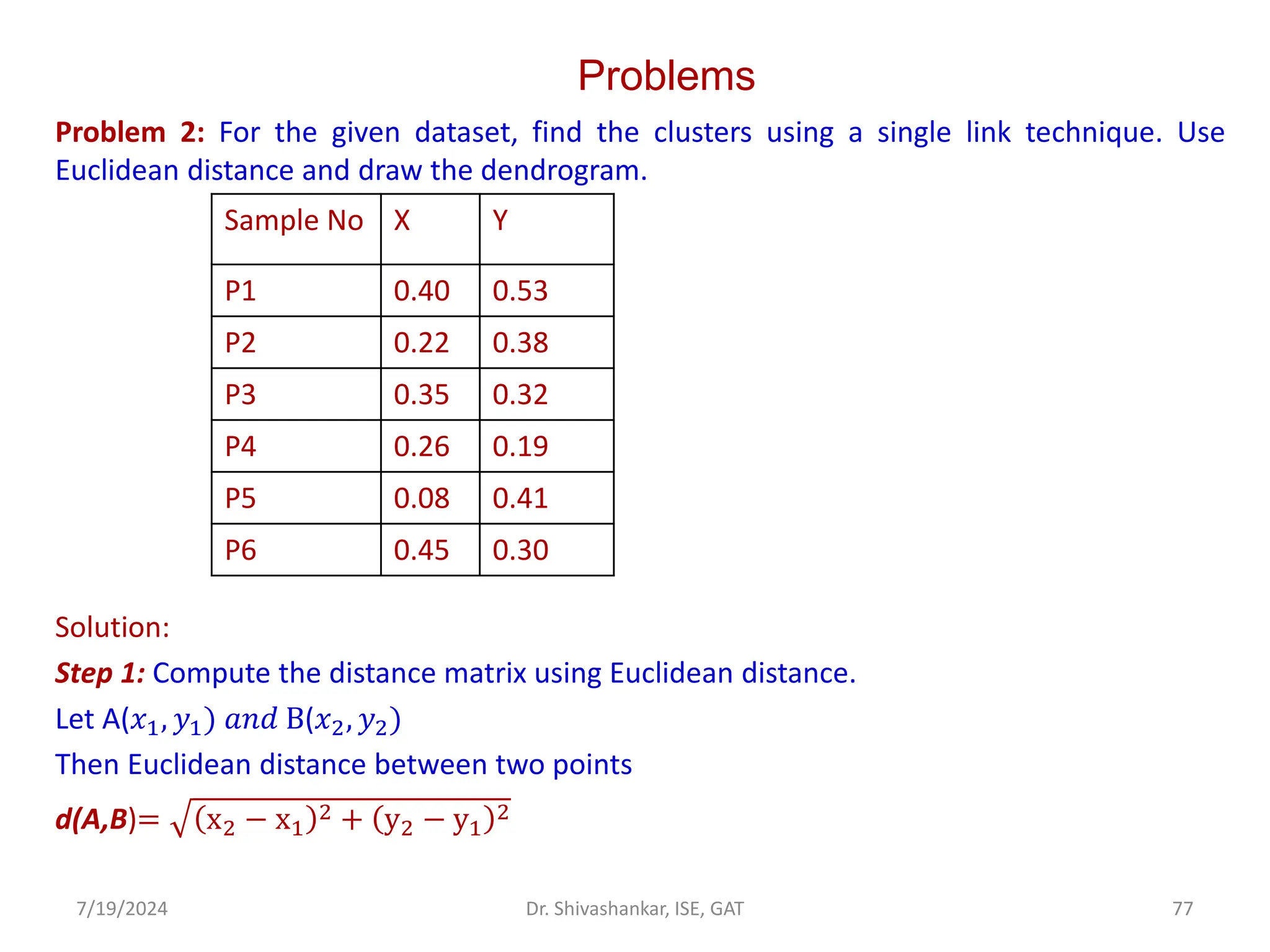
![Conti..
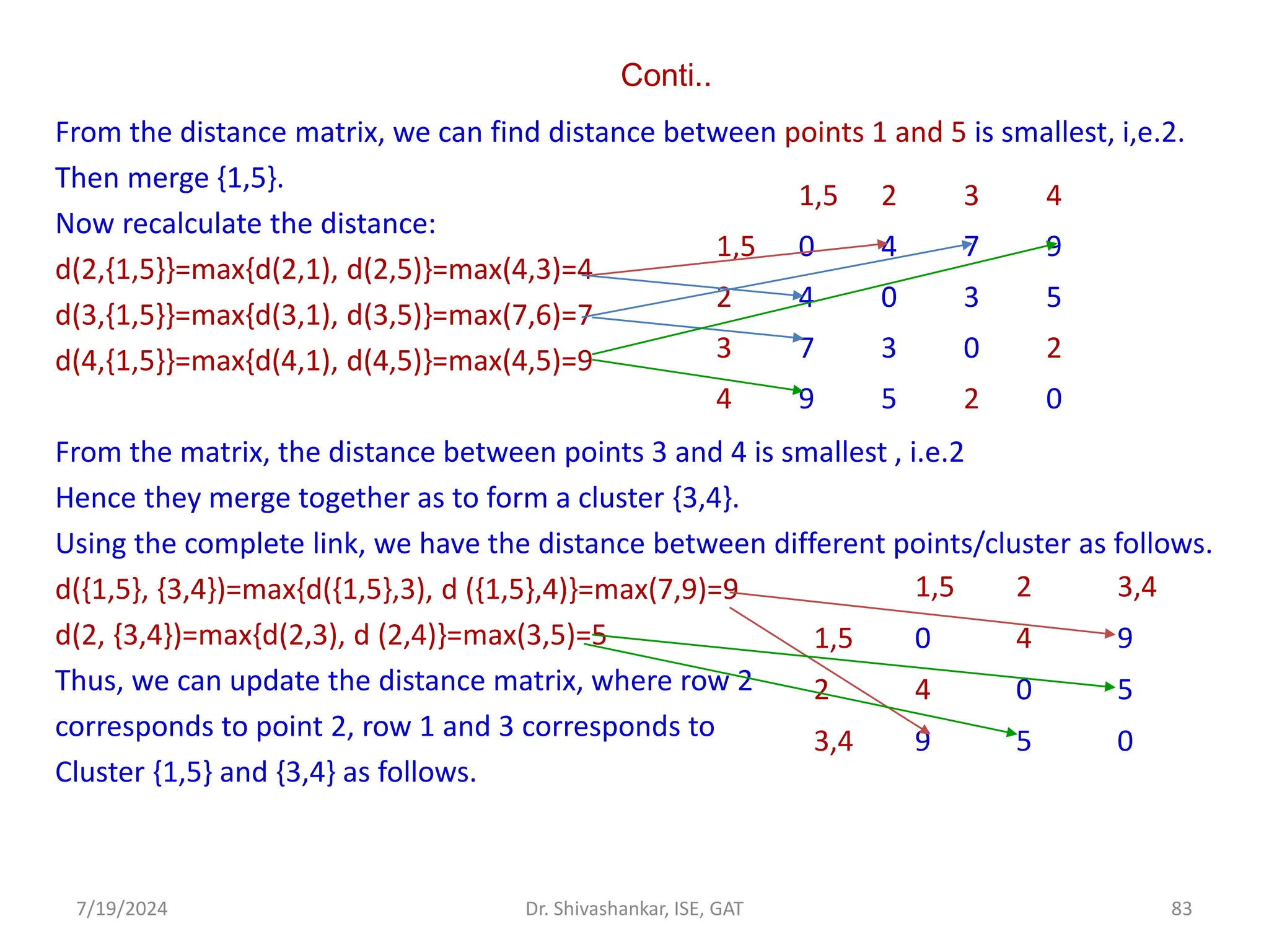
Following the same procedure, we merge pints 2 with the cluster {1,5} to form {1,2,5} and
update the distance matrix as follows.
After increase the distance threshold to 9,
all clusters would merge.
Fig 12: Dendogram for the given datasets
7/19/2024 84
Dr. Shivashankar, ISE, GAT
[1,5],2 [3,4]
[1,5],2 0 9
[3,4] 9 0](https://image.slidesharecdn.com/machinelearning-module2-240719092301-aa976ed7/75/Machine-Learning_SVM_KNN_K-MEANSModule-2-pdf-84-2048.jpg)


![SVM Implementation in Python
In Python, an SVM classifier can be developed using the sklearn library.
Step 1: Load the important libraries
>> import pandas as pd
>> import numpy as np
>> import sklearn
>> from sklearn import svm
>> from sklearn.model_selection import train_test_split
>> from sklearn import metrics
Step 2: Import dataset and extract the X variables and Y separately.
>> df = pd.read_csv(“mydataset.csv”)
>> X = df.loc[:,[‘Var_X1’,’Var_X2’,’Var_X3’,’Var_X4’]]
>> Y = df[[‘Var_Y’]]
Step 3: Divide the dataset into train and test
>> X_train, X_test, y_train, y_test = train_test_split(X, Y, test_size = 0.3,
random_state=123)
Step 4: Initializing the SVM classifier mode
>> svm_clf = svm.SVC(kernel = ‘linear’)
7/19/2024 25
Dr. Shivashankar, ISE, GAT](https://crownmelresort.com/image.slidesharecdn.com/machinelearning-module2-240719092301-aa976ed7/75/Machine-Learning_SVM_KNN_K-MEANSModule-2-pdf-25-2048.jpg)


![Conti..
Euc-dist[(𝑥1, 𝑦1); (𝑥2, 𝑦2)= 𝑥2 − 𝑥1
2 + 𝑦2 − 𝑦1
2
Class A : [(6,5);(4,2)] = 4 − 6 2 + 2 − 5 2 = 3.6
Class B: [(6,5);(7,6)] = 7 − 6 2 + 6 − 5 2 =1.414
The test instance has smaller distance to class B
Hence, the class of this test instance is predicted as B.
Problem 4. Given the following training instances in the table, each having two attributes
(x1 and x2). Compute the class label for test instance 𝑡1 = 3,7 , using 3 nearest neighbors
(k=3).
7/19/2024 44
Dr. Shivashankar, ISE, GAT
Training
Instances
𝑥1 𝑥2 Output
𝐼1 7 7 0
𝐼2 7 4 0
𝐼3 3 4 1
𝐼4 1 4 1](https://crownmelresort.com/image.slidesharecdn.com/machinelearning-module2-240719092301-aa976ed7/75/Machine-Learning_SVM_KNN_K-MEANSModule-2-pdf-44-2048.jpg)


![Cont…
Problem 1: Divide the given sample data into two clusters [2] using K means algorithm
S={2,3,4,10,11,12,20,25,30}. Given K=2, for new data point 15, identify the cluster belongs
to.
Solution:
1. Choose 2 random clusters from the given data sets C1=4, C2=12.
2. Find the distance between given samples and centroids, put the sample in the nearest
cluster.
3. Repeat the same for all data points.
Cluster k1={2,3,4} -------------(2-4=2, 3-4=1, 4-4=0, 10-4=6,……..
2-12=10, 3-12=9, 5-12=7, 10-12=2,……..
so 2,3 and 4 are placed in cluster 1 as its distance is nearest
to C1=4 and
Cluster K2={10,11,12,20,25,30}
4. Compute new centroids
K1={2,3,4} K2={10,11,12,20,25,30}
C1={2+3+4/3}=3 C2={10+11+12+20+25+30}/6=18
So C1=3 C2=18
7/19/2024 56
Dr. Shivashankar, ISE, GAT](https://crownmelresort.com/image.slidesharecdn.com/machinelearning-module2-240719092301-aa976ed7/75/Machine-Learning_SVM_KNN_K-MEANSModule-2-pdf-56-2048.jpg)


![Cont…
Step 3: cluster 1 of C1={ (1,1), (2,1), (3,2)}
cluster 2 of C2={ (2,3), (4,3), (5,5)}
Step 4: Recalculate cluster center
C1=
1
3
[(1,1)+(2,1)+(3,2)]=
1
3
[6,4]= (2,1.33)
C2=
1
3
[(2,3)+(4,3)+(5,5)]=
1
3
[11,11]= (3.67,3.67)
Step 5: Repeat the step 2 until we get same cluster center or same cluster elements
7/19/2024 59
Dr. Shivashankar, ISE, GAT
Data points Distance from
C1(2,1.33)
Distance from
C2(3.67,3.67)
New clusters
(1,1) 1.05 3.78 C1
(2,1) 0.33 3.15 C1
(2,3) 1.67 1.8 C1
(3,2) 1.204 1.8 C1
(4,3) 2.605 0.75 C2
(5,5) 4.74 1.88 C2](https://crownmelresort.com/image.slidesharecdn.com/machinelearning-module2-240719092301-aa976ed7/75/Machine-Learning_SVM_KNN_K-MEANSModule-2-pdf-59-2048.jpg)
![Cont…
cluster 1 of C1={ (1,1), (2,1),(2,3), (3,2)}
cluster 2 of C2={ (4,3), (5,5)}
Step 6: Recalculate cluster center
C1=
1
4
[(1,1)+(2,1)+(2,3)+(3,2)]=
1
4
[8,7]= (2,1.75)
C2=
1
2
[(4,3)+(5,5)]=
1
2
[9,8]= (4.5,4)
Step 7: Repeat the step 2 until we get same cluster center or same cluster elements
Step 8: cluster 1 of C1={ (1,1), (2,1),(2,3), (3,2)}
cluster 2 of C2={ (4,3), (5,5)}
Since cluster elements are same as compared to previous iteration, stop.
7/19/2024 60
Dr. Shivashankar, ISE, GAT
Data points Distance from C1(2,1.75) Distance from C2(4.5,4) New clusters
(1,1) 1.25 4.61 C1
(2,1) 0.75 3.9 C1
(2,3) 1.25 2.69 C1
(3,2) 1.03 2.5 C1
(4,3) 2.36 1.12 C2
(5,5) 4.42 1.12 C2](https://crownmelresort.com/image.slidesharecdn.com/machinelearning-module2-240719092301-aa976ed7/75/Machine-Learning_SVM_KNN_K-MEANSModule-2-pdf-60-2048.jpg)


![Agglomerative Hierarchical Clustering Algorithm
• Step 1: Consider each dataset as a single cluster and calculate the distance of
one cluster from all the other clusters.
• Step 2: In the second step, comparable clusters are merged together to form
a single cluster. Let’s say cluster (B) and cluster (C) are very similar to each
other, therefore we merge them in the second step similarly to cluster (D)
and (E) and at last, we get the clusters [(A), (BC), (DE), (F)]
• Step 3: We recalculate the proximity according to the algorithm and merge
the two nearest clusters([(DE), (F)]) together to form new clusters as [(A),
(BC), (DEF)]
• Step 4: Repeating the same process; The clusters DEF and BC are comparable
and merged together to form a new cluster. We’re now left with clusters [(A),
(BCDEF)].
• Step 4: At last, the two remaining clusters are merged together to form a
single cluster [(ABCDEF)].
7/19/2024 71
Dr. Shivashankar, ISE, GAT](https://crownmelresort.com/image.slidesharecdn.com/machinelearning-module2-240719092301-aa976ed7/75/Machine-Learning_SVM_KNN_K-MEANSModule-2-pdf-71-2048.jpg)


![Exercise problems
Since 3 is minimum distance, merge 22,25.and 27---{22,(25,27)}
Since 4 is minimum distance, merge 18,22,25,27---[18,{22,(25,27)}]
Draw the dendrogram for the merged data points.
7/19/2024 76
Dr. Shivashankar, ISE, GAT
18 22 25,27 42,43
18 0 4 7 24
22 4 0 3 20
25,27 7 3 0 15
42,43 24 20 15 0
18 22,25,27 42,43
18 0 4 24
22,25,27 4 0 15
42,43 24 15 0](https://crownmelresort.com/image.slidesharecdn.com/machinelearning-module2-240719092301-aa976ed7/75/Machine-Learning_SVM_KNN_K-MEANSModule-2-pdf-76-2048.jpg)


![Conti..
Now combined P2 and P5
[{(P3, P6), P4},(P2,P5)]
Now update the matrix and merge P2,P5,P3,P6 and P4
([{(P3, P6), P4},(P2,P5)], P1)
Now we have reached to the solution.
7/19/2024 80
Dr. Shivashankar, ISE, GAT
P1 P2 P3,P6,P4 P5
P1 0
P2 0.23 0
P3,P6,P4 0.22 0.14 0
P5 0.34 0.14 0.28 0
P1 P2,P5 P3,P6,P4
P1 0
P2,P5 0.23 0
P3,P6,P4 0.22 0.14 0
P1 P2,P5 P3,P6,P4
P1 0
P2,P5 0.23 0
P3,P6,P4 0.22 0.14 0
P1 P2,P5,P3,P6,P
4
P1 0
P2,P5,P3,P6,P4 0.22 0](https://crownmelresort.com/image.slidesharecdn.com/machinelearning-module2-240719092301-aa976ed7/75/Machine-Learning_SVM_KNN_K-MEANSModule-2-pdf-80-2048.jpg)


![Conti..
Following the same procedure, we merge pints 2 with the cluster {1,5} to form {1,2,5} and
update the distance matrix as follows.
After increase the distance threshold to 9,
all clusters would merge.
Fig 12: Dendogram for the given datasets
7/19/2024 84
Dr. Shivashankar, ISE, GAT
[1,5],2 [3,4]
[1,5],2 0 9
[3,4] 9 0](https://crownmelresort.com/image.slidesharecdn.com/machinelearning-module2-240719092301-aa976ed7/75/Machine-Learning_SVM_KNN_K-MEANSModule-2-pdf-84-2048.jpg)


![SVM[Support vector Machine] Machine learning](https://cdn.slidesharecdn.com/ss_thumbnails/svm-250403184638-1cd9afdb-thumbnail.jpg?width=640&height=640&fit=bounds)


