MACHINE LEARNING
(22ISE62)
Module 3
Dr.Shivashankar
Professor
Department of Information Science & Engineering
GLOBAL ACADEMY OF TECHNOLOGY-Bengaluru
24-05-2025 1
GLOBAL ACADEMY OF TECHNOLOGY
Ideal Homes Township, Rajarajeshwari Nagar, Bengaluru – 560 098
Department of Information Science & Engineering
Dr. Shivashankar-ISE-GAT
2.
Course Outcomes
After Completionof the course, student will be able to:
22ISE62.1: Describe the machine learning techniques, their types and data analysis framework.
22ISE62.2: Apply mathematical concepts for feature engineering and perform dimensionality
reduction to enhance model performance.
22ISE62.3: Develop similarity-based learning models and regression models for solving
classification and prediction tasks.
22ISE62.4: Build probabilistic learning models and design neural network models using perceptron
and multilayer architectures.
22ISE62.5: Utilize clustering algorithms to identify patterns in data and implement reinforcement
learning techniques.
Text Book:
1. S Sridhar, M Vijayalakshmi, “Machine Learning”, OXFORD University Press 2021, First Edition.
2. Murty, M. N., and V. S. Ananthanarayana. Machine Learning: Theory and Practice, Universities Press, 2024.
3. T. M. Mitchell, “Machine Learning”, McGraw Hill, 1997.
4. Burkov, Andriy. The hundred-page machine learning book. Vol. 1. Quebec City, QC, Canada: Andriy Burkov,
2019.
24-05-2025 2
Dr. Shivashankar-ISE-GAT
3.
Module 3- Similarity-basedLearning
• Similarity-based Learning is a supervised learning technique that predicts the class label
of a test instance by gauging the similarity of this test instance with training instances.
• Similarity-based learning refers to a family of instance-based learning which is used to
solve both classification and regression problems.
• Instance-based learning makes prediction by computing distances or similarities
between test instance and specific set of training instances local to the test instance in
an incremental process.
• This learning mechanism simply stores all data and uses it only when it needs to classify
an unseen instance.
• The advantage of using this learning is that processing occurs only when a request to
classify a new instance is given. This methodology is particularly useful when the whole
dataset is not available in the beginning but collected in an incremental manner.
• The drawback of this learning is that it requires a large memory to store the data since a
global.
24-05-2025 3
Dr. Shivashankar-ISE-GAT
4.
Nearest-Neighbor Learning
• Anon-parametric method used for both classification and regression problems.
• It is a simple and powerful non-parametric algorithm that predicts the category of the test instance according
to the ‘k’ training samples which are closer to the test instance and classifies it to that category which has the
largest probability.
• There are two classes of objects called 𝐶1 and 𝐶2.
• When given a test instance T, the category of this test instance is determined by looking at the class of k = 3
nearest neighbors.
• Thus, the class of this test instance T is predicted as C2.
• The algorithm classifies a new instance by determining the ‘k’
most similar instances (i.e., k nearest neighbors) and summarizing the output
of those ‘k’ instances.
• If the target variable is discrete then it is a classification problem,
so it selects the most common class value among the ‘k’ instances by
a majority vote.
• However, if the target variable is continuous then it is a regression
problem, and hence the mean output variable of the ‘k’ instances is the
output of the test instance.
24-05-2025 4
Dr. Shivashankar-ISE-GAT
Figure 4.1: Visual Representation of
k-Nearest Neighbor Learning
5.
Conti..
Inputs: Training datasetT, distance metric d, Test instance t, the number of nearest neighbors k
Output: Predicted class or category
Prediction: For test instance t:
1. For each instance i in T, compute the distance between the test instance t and every other instance i in the
training dataset using a distance metric (Euclidean distance).
[Continuous attributes - Euclidean distance between two points in the plane with coordinates (𝑥1, 𝑦1) and (𝑥2, 𝑦2)
is given as dist
((𝑥1, 𝑦1), (𝑥2, 𝑦2)) = 𝑥2 − 𝑥1
2 + 𝑦2 − 𝑦1
2
If the value of the two instances is same, the distance d =0 otherwise d = 1.
2. Sort the distances instances to the test instance in an ascending order and select the first k nearest training data
3. Predict the class of the test instance by majority voting (if target attribute is discrete valued) or mean (if target
attribute is continuous valued) of the k selected nearest instances.
24-05-2025 5
Dr. Shivashankar-ISE-GAT
6.
Conti..
Problem 1: Considerthe student performance training dataset of 8 data instances shown in Table, which
describes the performance of individual students in a course and their CGPA obtained in the previous
semesters. The independent attributes are CGPA, Assessment and Project. The target variable is ‘Result’
which is a discrete valued variable that takes two values ‘Pass’ or ‘Fail’. Based on the performance of a
student, classify whether a student will pass or fail in that course. Using K-NN algorithm and instances ((6.1,
40, 5).
24-05-2025 6
Dr. Shivashankar-ISE-GAT
Sl. No. CGPA Assessment Project
Submitted
Result
1 9.2 85 8 Pass
2 8 80 7 Pass
3 8.5 81 8 Pass
4 6 45 5 Fail
5 6.5 50 4 Fail
6 8.2 72 7 Pass
7 5.8 38 5 Fail
8 8.9 91 9 Pass
7.
Conti..
Solution: Given atest instance (6.1, 40, 5) and a set of categories {Pass, Fail} also called as classes, we need
to use the training set to classify the test instance using Euclidean distance.
The task of classification is to assign a category or class to an arbitrary instance. Assign k = 3 (CGPA,
Assessment and project submitted .
Step 1: Calculate the Euclidean distance between the test instance (6.1, 40, and 5) and each of the training
instances as shown in Table 4.1.
24-05-2025 7
Dr. Shivashankar-ISE-GAT
Sl.
No.
CGPA Assessment Project
Submitted
Result Euclidean distance
1 9.2 85 8 Pass 9.2 − 6.1 2 + 85 − 40 2 + 8 − 5 2= 45.2063
2 8 80 7 Pass 8 − 6.1 2 + 80 − 40 2 + 7 − 5 2= 40.09501
3 8.5 81 8 Pass 8.5 − 6.1 2 + 81 − 40 2 + 8 − 5 2= 41.17961
4 6 45 5 Fail 6 − 6.1 2 + 45 − 40 2 + 5 − 5 2= 5.001
5 6.5 50 4 Fail 6.5 − 6.1 2 + 50 − 40 2 + 4 − 5 2= 10.0578
6 8.2 72 7 Pass 8.2 − 6.1 2 + 72 − 40 2 + 7 − 5 2= 32.13114
7 5.8 38 5 Fail 5.8 − 6.1 2 + 38 − 40 2 + 5 − 5 2= 2.022375
8 8.9 91 9 Pass 8.9 − 6.1 2 + 91 − 40 2 + 9 − 5 2= 51.23319
8.
Conti..
Step 2: Sortthe distances in the ascending order and select the first 3 nearest
training data instances to the test instance.
Table 4.4: Nearest Neighbors Instance Euclidean Distance.
Here, we take the 3 nearest neighbors as instances 4, 5 and 7 with smallest
distances.
Step 3: Predict the class of the test instance by majority voting.
The class for the test instance is predicted as ‘Fail’.
24-05-2025 8
Dr. Shivashankar-ISE-GAT
Instance Euclidean distance Class
4 5.001 Fail
5 10.0578 Fail
7 2.022375 Fail
9.
Conti..
Problem 2: Fromthe given dataset, find (x,y)= (170, 57) whether belongs to under or normal weight. Assume K=3.
Solution:
Find the Euc-dist:d= 𝑥2 − 𝑥1
2 + 𝑦2 − 𝑦1
2
d1= 170 − 167 2 + 57 − 51 2
= 32 + 62 = 45 = 6.70
d2= 122 + 52 = 169 =13
And so on till d10
5/24/2025 9
Dr. Shivashankar, ISE, GAT
Height (cm) Weight (kg) Class
167 51 Underweight
182 62 Normal
176 69 Normal
173 64 Normal
172 65 Normal
174 56 Underweight
169 58 Normal
173 57 Normal
170 55 Normal
170 57 ?
10.
Conti..
Since K=3, withmaximum 3 ranks
with distances.
The smallest distance is
• (169,58)-1.414: Normal
• (170,55)-2: Normal
• (173,57)-3:Normal
Hence all 3 points, so (170,57)belongs
to normal class,
5/24/2025 10
Dr. Shivashankar, ISE, GAT
Height (cm) Weight (kg) Class Distance
167 51 Underweight 6.7
182 62 Normal 13
176 69 Normal 13.4
173 64 Normal 7.6
172 65 Normal 8.2
174 56 Underweight 4.1
169 58 Normal 1.414-1(R)
173 57 Normal 3-3(R)
170 55 Normal 2-2(R)
170 57 Normal 3
11.
Conti..
Problem 2: Fromthe given dataset, find (x,y)= (157, 54) whether belongs to medium or longer. Assume
K=3.
5/24/2025 11
Dr. Shivashankar, ISE, GAT
Sl. No. Height Weight Target
1 150 50 Medium
2 155 55 Medium
3 160 60 Longer
4 161 59 Longer
5 158 65 Longer
6 157 54 ?
12.
Conti..
Problem 3: Fromthe given dataset, find (x,y)= (5.2, 3.1),using KNN Classifier to classify New Instance IRIS
5/24/2025 12
Dr. Shivashankar, ISE, GAT
Sepal length Sepal width Species
5.3 3.7 Setosa
5.1 3.8 Setosa
7.2 3.0 Virgina
5.4 3.4 Setosa
5.1 3.3 Setosa
5.4 3.9 Setosa
7.4 2.8 Virgina
6.1 2.8 Verscicolor
7.3 2.9 Virgina
6.0 2.7 Verscicolor
5.8 2.8 Virgina
6.3 2.3 Verscicolor
5.1 2.5 Verscicolor
6.3 2.5 Verscicolor
5.5 2.4 Verscicolor
13.
Weighted K-Nearest-Neighbor Algorithm
•The Weighted k-NN is an extension of k-NN.
• It chooses the neighbors by using the weighted distance.
• The k-Nearest Neighbor (k-NN) algorithm has some serious limitations as its
performance is solely dependent on choosing the k nearest neighbors, the distance
metric used and the decision rule.
• However, the principle idea of Weighted k-NN is that k closest neighbors to the test
instance are assigned a higher weight in the decision as compared to neighbors that are
farther away from the test instance.
• The idea is that weights are inversely proportional to distances.
• The selected k nearest neighbors can be assigned uniform weights, which means all the
instances in each neighborhood are weighted equally or weights can be assigned by the
inverse of their distance.
• In the second case, closer neighbors of a query point will have a greater influence than
neighbors which are further away.
24-05-2025 13
Dr. Shivashankar-ISE-GAT
14.
Conti..
Algorithm 4.2: Weightedk-NN
Inputs: Training dataset ‘T’, Distance metric ‘d’, Weighting function w(i), Test instance ‘t’, the number of nearest neighbors ‘k’
Output: Predicted class or category Prediction: For test instance t,
1. For each instance ‘i’ in Training dataset T, compute the distance between the test instance t and every other instance ‘i’
using a distance metric (Euclidean distance). [Continuous attributes - Euclidean distance between two points in the plane
with coordinates (𝑥1, 𝑦1) and (𝑥2, 𝑦2) is given as dist
((𝑥1, 𝑦1), (𝑥2, 𝑦2)) = 𝑥2 − 𝑥1
2 + 𝑦2 − 𝑦1
2
If the value of the two instances is same, the distance d =0 otherwise d = 1.
2. Sort the distances in the ascending order and select the first ‘k’ nearest training data instances to the test instance.
3. Predict the class of the test instance by weighted voting technique (Weighting function w(i)) for the k selected nearest
instances:
• Compute the inverse of each distance of the ‘k’ selected nearest instances.
• Find the sum of the inverses.
• Compute the weight by dividing each inverse distance by the sum. (Each weight is a vote for its associated class).
• Add the weights of the same class.
• Predict the class by choosing the class with the maximum vote.
24-05-2025 14
Dr. Shivashankar-ISE-GAT
15.
Conti..
Example 4.2: Considerthe same training dataset given in Table 4.1. Use Weighted k-NN and determine the
class.
Solution: Step 1: Given a test instance (7.6, 60, 8) and a set of classes {Pass, Fail}, use the training dataset to
classify the test instance using Euclidean distance and weighting function.
Assign k = 3.
24-05-2025 15
Dr. Shivashankar-ISE-GAT
Sl. No. CGPS Assessment Project
Submitted
Result Euclidean distance
1 9.2 85 8 Pass 9.2 − 7.6 2 + 85 − 60 2 + 8 − 8 2= 25.05115
2 8 80 7 Pass 8 − 7.6 2 + 80 − 60 2 + 7 − 8 2= 20.0898
3 8.5 81 8 Pass 8.5 − 7.6 2 + 81 − 60 2 + 8 − 8 2= 21.01928
4 6 45 5 Fail 6 − 7.6 2 + 45 − 60 2 + 5 − 8 2= 15.38051
5 6.5 50 4 Fail 6.5 − 7.6 2 + 50 − 60 2 + 4 − 8 2= 10.82636
6 8.2 72 7 Pass 8.2 − 7.6 2 + 72 − 60 2 + 7 − 8 2= 12.05653
7 5.8 38 5 Fail 5.8 − 7.6 2 + 38 − 60 2 + 5 − 8 2= 22.27644
8 8.9 91 9 Pass 8.9 − 7.6 2 + 91 − 60 2 + 9 − 8 2= 31.04336
16.
Conti..
Step 2: Sortthe distances in the ascending order and select the first 3 nearest training data instances to the
test instance.
Table 4.6: Nearest Neighbors Instance Euclidean
Step 3: Predict the class of the test instance by weighted voting technique from the 3 selected nearest
instances.
• Compute the inverse of each distance of the 3 selected nearest instances as shown in Table 4.7.
Table 4.7: Inverse Distance Instance Euclidean
24-05-2025 16
Dr. Shivashankar-ISE-GAT
Instance Euclidean distance Class
4 15.38051 Fail
5 10.82636 Fail
6 12.05653 Pass
Instance Euclidean distance Inverse distance (1/ED) Class
4 15.38051 0.06502 Fail
5 10.82636 0.092370 Fail
6 12.05653 0.08294 Pass
17.
Conti..
• Find thesum of the inverses. Sum = 0.06502 + 0.092370 + 0.08294 = 0.24033
• Compute the weight by dividing each inverse distance by the sum as shown in Table 4.8.
Table 4.8: Weight Calculation Instance Euclidean Distance
• Add the weights of the same class.
Fail = 0.270545 + 0.384347 = 0.654892
Pass = 0.345109
• Predict the class by choosing the class with the maximum vote.
The class is predicted as ‘Fail’.
24-05-2025 17
Dr. Shivashankar-ISE-GAT
Instance Euclidean
distance
Inverse
distance
Distance Weight =
Inverse distance/Sum
Class
4 15.38051 0.06502 0.270545 Fail
5 10.82636 0.092370 0.384347 Fail
6 12.05653 0.08294 0.34510 Pass
18.
Conti..
Problem 2: Giventhe following training instances, each having two attributers (x1 and x2). Compute class
label for test instance t1 = (3,7) using three nearest neighbors (k=3).
Solution:
24-05-2025 18
Dr. Shivashankar-ISE-GAT
Training Instance x1 x2 output
I1 7 7 0
I2 7 4 0
I3 3 4 1
I4 1 4 1
Training
Instance
x1 x2 output ED 𝑑2 Vote
(1/d)
Rank
I1 7 7 0 4 16 0.06 3
I2 7 4 0 5 25 0.04 4
I3 3 4 1 3 9 0.11 1
I4 1 4 1 3.6 12.96 0.08 2
19.
Nearest Centroid Classifier
•A simple and efficient machine learning algorithm used for classification.
• It works by calculating the centroid (mean) of each class in the training data and then assigning a new
data point to the class whose centroid is closest to it.
• This algorithm is also known as Minimum Distance Classifier or Centroid-based Classification.
• A simple alternative to k-NN classifiers for similarity-based classification is the Nearest Centroid Classifier.
• It is a simple classifier and also called as Mean Difference classifier.
• The idea of this classifier is to classify a test instance to the class whose centroid/mean is closest to that
instance.
Algorithm 4.3: Nearest Centroid Classifier
Inputs: Training dataset T, Distance metric d, Test instance t
Output: Predicted class or category
1. Compute the mean/centroid of each class.
2. Compute the distance between the test instance and mean/centroid of each class (Euclidean
Distance).
3. Predict the class by choosing the class with the smaller distance.
24-05-2025 19
Dr. Shivashankar-ISE-GAT
20.
Conti..
Problem 1: Considerthe sample data shown in Table 4.9 with two features x and y. The target classes are ‘A’
or ‘B’ with given instance (6, 5), Predict the class using Nearest Centroid Classifier.
Table 4.9: Sample Data X Y
Solution:
Step 1: Compute the mean/centroid of each class. In this example there are two classes called ‘A’ and ‘B’.
24-05-2025 20
Dr. Shivashankar-ISE-GAT
x y Class
3 1 A
5 2 A
4 3 A
7 6 B
6 7 B
8 5 B
21.
Conti..
Centroid of class‘A’ = (3 + 5 + 4, 1 + 2 + 3)/3 = (12, 6)/3 = (4, 2)
Centroid of class ‘B’ = (7 + 6 + 8, 6 + 7 + 5)/3 = (21, 18)/3 = (7, 6)
Now given a test instance (6, 5), we can predict the class.
Step 2: Calculate the Euclidean distance between test instance (6, 5) and each of the centroid.
Euc_Dist[(6, 5); (4, 2)] = 6 − 4 2 + 5 − 2 2= 3.6
Euc_Dist[(6, 5); (7, 6)] = 6 − 7 2 + 5 − 6 2= 1.414
The test instance has smaller distance to class B. Hence, the class of this test instance is predicted as ‘B’.
24-05-2025 21
Dr. Shivashankar-ISE-GAT
22.
Conti..
Problem 2: Considerthe following training dataset of 10 data instances shown in Table with new instance
(7.8, 4), k=3 which describes the award performance of individual students based on GPA and No. of
projects done. The target variable is ‘Award’ which is a discrete valued variable that takes 2 values ‘Yes’ or
‘No’. Apply k-Nearest Neighbor classifier, Weighted k-Nearest Neighbor classifier and Nearest Centroid
Classifier
Table 4.12: Training Dataset
.
24-05-2025 22
Dr. Shivashankar-ISE-GAT
Sl. No. GPA No. of projects
done
Award
1 9.5 5 Yes
2 8.0 4 Yes
3 7.2 1 No
4 6.5 5 Yes
5 9.5 4 Yes
6 3.2 1 No
7 6.6 1 No
8 5.4 1 No
9 8.9 3 Yes
10 7.2 4 Yes
23.
Locally Weighted Regression
•Locally Weighted Regression (LWR) is a non-parametric supervised learning algorithm that
performs local regression by combining regression model with nearest neighbor’s model.
• LWR is also referred to as a memory-based method as it requires training data while prediction
but uses only the training data instances locally around the point of interest.
• Using nearest neighbors algorithm, we find the instances that are closest to a test instance and
fit linear function to each of those ‘k’ nearest instances in the local regression model.
• The key idea is that we need to approximate the linear functions of all ‘k’ neighbors that
minimize the error such that the prediction line is no more linear but rather it is a curve.
• Hypothesis function ℎ𝛽(x), the predicted target output is a linear function where 𝛽0 is the
intercept and 𝛽1 is the coefficient of x.
ℎ𝛽(𝑥)= 𝛽0 + 𝛽1𝑥
• The cost function is such that it minimizes the error difference between the predicted value
ℎ𝛽(𝑥) and true value ‘y’ and it is given as
𝐽(𝛽) =
1
2
𝑖=1
𝑚
𝑤𝑖 ℎ𝛽(𝑥𝑖)−𝑦𝑖
2
• Where 𝑤𝑖=exp −
𝑥𝑖−𝑥 2
2𝜏2 , where where, τ is called the bandwidth parameter and controls the
rate at which 𝑤𝑖 reduces to zero with distance from 𝑥𝑖.
24-05-2025 23
Dr. Shivashankar-ISE-GAT
24.
Conti..
Problem 1: Considera simple example with four instances shown in Table 4.10 and apply locally weighted regression. 𝛽0
= 4.72, 𝛽1= 0.62 Given a test instance with x = 2, 𝜏=0.4. Table 4.10: Sample Table
Solution: Using linear regression model assuming we have computed the parameters:
𝛽0 = 4.72, 𝛽1= 0.62 Given a test instance with x = 2, the predicted y’ is:
y’ = 𝛽0 + 𝛽1 x = 4.72 + 0.62 × 2 = 5.96
Applying the nearest neighbor model, we choose k = 3 closest instances (2,3,4 are similar).
24-05-2025 24
Dr. Shivashankar-ISE-GAT
Sl. No. Salary in lakh Expenditure (in thousands)
1 5 25
2 1 5
3 2 7
4 1 8
Sl. No. Salary in lakh Expenditure (in thousands) Euclidean distance
1 5 25 5 − 2 2 = 3
2 1 5 1 − 2 2 = 1
3 2 7 2 − 2 2 = 0
4 1 8 1 − 2 2 = 1
25.
Conti..
Instances 2, 3and 4 are closer with smaller distances. The mean value = (5 + 7 + 8)/3 =
20/3 = 6.67. Compute the weights for the closest instances, using the Gaussian kernel
𝑤𝑖=exp −
𝑥𝑖−𝑥 2
2𝜏2
Weight of Instance 2:
𝑤2=exp −
𝑥2−𝑥 2
2𝜏2 = exp −
1−2 2
2𝑥0.42 = 𝑒−3.125= 0.043
Weight of Instance 3:
𝑤3=exp −
𝑥3−𝑥 2
2𝜏2 = exp −
2−2 2
2𝑥0.42 = 𝑒0= 1
Weight of Instance 4:
𝑤4=exp −
𝑥4−𝑥 2
2𝜏2 = exp −
1−2 2
2𝑥0.42 = 𝑒−3.125= 0.043
𝑒0
= 1 [𝑤3 is closer hence gets a higher weight value]
24-05-2025 25
Dr. Shivashankar-ISE-GAT
26.
Conti..
The predicted outputfor the three closer instances is given as follows:
The predicted output of Instance 2 is:
𝑦2
′
=ℎ𝛽 𝑥2 = 𝛽0 + 𝛽1𝑥2 = 4.72 + 0.62 × 1 = 5.34
The predicted output of Instance 3 is:
𝑦3
′
=ℎ𝛽 𝑥3 = 𝛽0 + 𝛽1𝑥3= 4.72 + 0.62 × 2 = 5.96
𝑇ℎ𝑒 𝑝𝑟𝑒𝑑𝑖𝑐𝑡𝑒𝑑 𝑜𝑢𝑡𝑝𝑢𝑡 𝑜𝑓 𝐼𝑛𝑠𝑡𝑎𝑛𝑐𝑒 4 𝑖𝑠:
𝑦4
′
=ℎ𝛽 𝑥4 = 𝛽0 + 𝛽1𝑥4 = 4.72 + 0.62 × 1 = 5.34
𝑤𝑒 𝑛𝑒𝑒𝑑 𝑡𝑜 𝑎𝑑𝑗𝑢𝑠𝑡 𝑡ℎ𝑖𝑠 𝑐𝑜𝑠𝑡 𝑓𝑢𝑛𝑐𝑡𝑖𝑜𝑛 𝑡𝑜 𝑚𝑖𝑛𝑖𝑚𝑖𝑧𝑒 𝑡ℎ𝑒 𝑒𝑟𝑟𝑜𝑟 𝑑𝑖𝑓𝑓𝑒𝑟𝑒𝑛𝑐𝑒
𝑎𝑛𝑑 𝑔𝑒𝑡 𝑜𝑝𝑡𝑖𝑚𝑎𝑙 𝛽 𝑝𝑎𝑟𝑎𝑚𝑒𝑡𝑒𝑟𝑠.
𝐽 𝛽 =
1
2
𝑖=1
𝑚
𝑤𝑖 ℎ𝛽 𝑥𝑖 −𝑦𝑖
2
=
1
2
0.043(5.34−5 2 + 1 5.96 − 7 2 + 0.043(5.34−8 2
= 0.6953
24-05-2025 26
Dr. Shivashankar-ISE-GAT
27.
Regression Analysis
Introduction toRegression:
• Regression in machine learning is a technique that uses statistical methods to predict
continuous outcomes based on input data.
• It's a supervised learning technique, which means that it's trained on labeled data.
• Given a training dataset D containing N training points (𝑥𝑖, 𝑦𝑖), where i = 1...N,
regression analysis is used to model the relationship between one or more independent
variables 𝑥𝑖 and a dependent variable 𝑦𝑖.
• The relationship between the dependent and independent variables can be represented
as a function as follows:
y = f(x)
• Here, the feature variable x is also known as an explanatory variable, exploratory
variable, a predictor variable, an independent variable, a covariate, or a domain point.
• y is a dependent variable.
• Dependent variables are also called as labels, target variables, or response variables.
24-05-2025 27
Dr. Shivashankar-ISE-GAT
28.
Conti..
• Regression analysisdetermines the change in response variables when one
exploration variable is varied while keeping all other parameters constant.
• This is used to determine the relationship each of the exploratory variables
exhibits.
• Thus, regression analysis is used for prediction and forecasting.
There are many applications of regression analysis. Some of the applications
of regressions include predicting:
1. Sales of a goods or services
2. Value of bonds in portfolio management
3. Premium on insurance companies
4. Yield of crops in agriculture 5. Prices of real estate
24-05-2025 28
Dr. Shivashankar-ISE-GAT
29.
INTRODUCTION TO LINEARITY,CORRELATION, AND CAUSATION
• The quality of the regression analysis is determined by the factors such as correlation and causation.
Regression and Correlation
• Correlation among two variables can be done effectively using a Scatter plot, which is a plot between explanatory
variables and response variables.
• It is a 2D graph showing the relationship between two variables.
• The x-axis of the scatter plot is independent, or input or predictor variables and y-axis of the scatter plot is output or
dependent or predicted variables.
The scatter plot is useful in exploring data.
• A correlation coefficient, ranging from -1 to +1, quantifies this relationship, with values close to +1 representing a
strong positive correlation, close to -1 a strong negative correlation, and close to 0 no linear correlation.
24-05-2025 29
Dr. Shivashankar-ISE-GAT
Figure 5.1: Examples of (a) Positive Correlation (b)
Negative Correlation (c) Random Points with No
Correlation
30.
Conti..
Causation:
• It isthe process of identifying and understanding cause-effect relationships between variables.
• Causation is about causal relationship among variables, say x and y.
• It means knowing whether x causes y to happen or vice versa. x causes y is often denoted as x
implies y.
• Correlation and Regression relationships are not same as causation relationship.
• For example, the correlation between economical background and marks scored does not imply
that economic background causes high marks.
• Similarly, the relationship between higher sales of cool drinks due to a rise in temperature is not
a causal relation.
• Even though high temperature is the cause of cool drinks sales, it depends on other factors too.
24-05-2025 30
Dr. Shivashankar-ISE-GAT
31.
Linearity and Non-linearityRelationships
• Linear relationships exhibit a constant rate of change, represented by a straight line on a graph, where a
change in one variable directly corresponds to a proportional change in another.
• The linearity relationship between the variables means the relationship between the dependent and
independent variables can be visualized as a straight line.
• The line of the form, y = ax + b can be fitted to the data points that indicate the relationship between x
and y.
• By linearity, it is meant that as one variable increases, the corresponding variable also increases in a linear
manner.
• Figure 5.2: (a) Example of Linear Relationship of the Form y = ax + b (b) Example of a Non-linear
Relationship of the Form y = a𝑥𝑏 (c) Examples of a Non-linear Relationship y =
𝑥
𝑎𝑥+𝑏
24-05-2025 31
Dr. Shivashankar-ISE-GAT
32.
Conti..
24-05-2025 32
Dr. Shivashankar-ISE-GAT
Figure5.2: (a) Example of Linear Relationship of the Form y = ax + b (b) Example of a Non-linear Relationship of the
Form y = a𝑥𝑏
(c) Examples of a Non-linear Relationship y =
𝑥
𝑎𝑥+𝑏
33.
Introduction to LinearRegression
The linear regression model can be created by fitting a line among the scattered data points. The line is of
the form defined as
Y=𝑎0 + 𝑎1𝑥 + 𝑒
𝑎0 is the intercept which represents the bias and 𝑎1 represents the slope of the line.
These are called regression coefficients. e is the error in prediction.
The assumptions of linear regression are listed as follows:
1. The observations (y) are random and are mutually independent.
2. The difference between the predicted and true values is called an error. The error is also mutually
independent with the same distributions such as normal distribution with zero mean and constant
variables.
3. The distribution of the error term is independent of the joint distribution of explanatory variables.
4. The unknown parameters of the regression models are constants.
• The idea of linear regression is based on Ordinary Least Square (OLS) approach.
• This method is also known as ordinary least squares method.
• In this method, the data points are modelled using a straight line.
24-05-2025 33
Dr. Shivashankar-ISE-GAT
34.
Conti..
• In figure,three data points and their errors (e1, e2, e3) are shown.
• The vertical distance between each point and the line (predicted by the approximate line equation y = a0
+ a1 x) is called an error.
• These individual errors are added to compute the total error of the predicted line. This is called sum of
residuals.
• The squares of the individual errors can also be computed and added to give a sum of squared error.
• The line with the lowest sum of squared error is called line of best fit.
Figure 5.4: Data Points and their Errors
24-05-2025 34
Dr. Shivashankar-ISE-GAT
35.
Conti..
The line equationsfor points (x1, x2, …, xn) are:
𝑦1 = (𝑎0 + 𝑎1𝑥1+𝑒1)
𝑦1 = (𝑎0 + 𝑎1𝑥2+𝑒2)
𝑦1 = (𝑎0 + 𝑎1𝑥3+𝑒3)
.
.
.
𝑦1 = (𝑎0 + 𝑎1𝑥𝑛+𝑒𝑛)
In general, the error is given as: 𝑒𝑖 = 𝑦𝑖- (𝑎0 + 𝑎1𝑥𝑖)
The residuals (𝑒𝑖) can be positive, negative or zero.
A regression line is the line of best fit for which the sum of the squares of residuals is minimum.
The minimization can be done as minimization of individual errors by finding the parameters 𝑎0 and 𝑎1 such
that:
𝐸 =
𝑖=1
𝑛
𝑒𝑖 =
𝑖=1
𝑛
𝑦𝑖− (𝑎0 + 𝑎1𝑥𝑖)
24-05-2025 35
Dr. Shivashankar-ISE-GAT
36.
Conti..
The minimization ofthe sum of the squares of the individual errors:
𝐸 =
𝑖=1
𝑛
𝑒𝑖
2
=
𝑖=1
𝑛
𝑦𝑖 − 𝑎0 + 𝑎1𝑥𝑖
2
Therefore, linear regression is modelled as a minimization function as follows:
𝐽 𝑎1, 𝑎0 =
𝑖=1
𝑛
𝑦𝑖 − 𝑓 𝑥𝑖
2
=
𝑖=1
𝑛
𝑦𝑖 − 𝑎0 + 𝑎1𝑥𝑖
2
Here, 𝐽 𝑎1, 𝑎0 is the criterion function of parameters 𝑎0 and 𝑎1.
This needs to be minimized.
This is done by differentiating and substituting to zero.
The values of estimates of 𝑎0and 𝑎1 are given as follows:
𝑎1 =
𝑥𝑦 − ҧ
𝑥 ത
𝑦
𝑥𝑖
2
− ҧ
𝑥 2
and
𝑎0 = ത
𝑦 − 𝑎1𝑋 ҧ
𝑥
24-05-2025 36
Dr. Shivashankar-ISE-GAT
37.
Introduction to LinearRegression
Problem 1: Let us consider an example where the five weeks' sales data (in Thousands) is given as shown
below in Table 5.1. Apply linear regression technique to predict the 7th and 12th month sales.
24-05-2025 37
Dr. Shivashankar-ISE-GAT
𝑥𝑖
Week
𝑦𝑖
Sales in Thousands
1 1.2
2 1.8
3 2.6
4 3.2
5 3.8
38.
Conti..
𝑥𝑖
Week
𝑦𝑖
Sales in Thousands
𝑥𝑖
2𝑥𝑖 x 𝑦𝑖
1 1.2 1 1.2
2 1.8 4 3.6
3 2.6 9 7.8
4 3.2 16 12.8
5 3.8 25 19
Average = ҧ
𝑥=
15
5
= 3 Average = ത
𝑦=
12.6
5
= 2.52 Average = 𝑥𝑖
2
=
55
5
= 11 Average (𝑥𝑖 x 𝑦𝑖) =𝑥𝑦 =
44.,4
5
= 8.88
24-05-2025 38
Dr. Shivashankar-ISE-GAT
Let us compute the slope and intercept as = 𝑎1 =
𝑥𝑦 − ҧ
𝑥 ത
𝑦
𝑥𝑖
2− ҧ
𝑥 2 =
8.88−3𝑥2.52
11−32 = 0.66
𝑎0 = ത
𝑦 − 𝑎1𝑥 ҧ
𝑥 = 2.52 – 0.66 x 3 = 0.54
Solution: Here, there are 5 samples, i.e., i = 1, 2, 3, 4, 5.
39.
Conti..
Figure 5.5: LinearRegression Model Constructed.
Therefore, the fitted line for the above data is: y = 0.54 +0.66x.
The predicted 7th week sale would be (when x = 7),
y = 0.54 + 0.66 × 7 = 5.16 and
the 12th month, y = 0.54 + 0.66 × 12 = 8.46.
24-05-2025 39
Dr. Shivashankar-ISE-GAT
Regression line (ො
𝑦= 0.66x +0.54)
40.
Conti..
Problem 2: Considerthe following dataset in Table 5.11 where the week and
number of working hours per week spent by a research scholar in a library
are tabulated. Based on the dataset, predict the number of hours that will be
spent by the research scholar in the 7th and 9th week. Apply linear
regression model.
24-05-2025 40
Dr. Shivashankar-ISE-GAT
𝑥𝑖 (Week) 1 2 3 4 5
𝑦𝑖 (Hours Spent) 12 18 22 28 35
41.
Linear Regression inMatrix Form
Matrix notations can be used for representing the values of independent and dependent variables.
This is illustrated as:
𝑦1
𝑦2
.
.
.
𝑦𝑛
=
1 𝑥1
1 𝑥2
.
.
.
1 𝑥𝑛
𝑎0
𝑎1
+
𝑒1
𝑒2
.
.
.
𝑒𝑛
This can be written as: Y = Xa + e, where X is an n × 2 matrix, Y is an n × 1 vector, a is a 2 × 1 column vector
and e is an n × 1 column vector.
24-05-2025 41
Dr. Shivashankar-ISE-GAT
42.
Conti..
Problem 1: Findlinear regression of the data of week and product sales (in Thousands). Use linear regression
in matrix form.
Table 5.3: Sample Data for Regression
Solution: Solution: The dependent variable X is be given as: 𝑥𝑇 = [1 2 3 4]
And the independent variable is given as follows: 𝑦𝑇 = [1 3 4 8]
The data can be given in matrix form as follows: X
1 1
1 2
1 3
1 4
and Y=
1
3
4
8
24-05-2025 42
Dr. Shivashankar-ISE-GAT
𝑥𝑖
Week
𝑦𝑖
Product Sales in Thousands
1 1
2 3
3 4
4 8
43.
Conti..
The regression isgiven as: a = ( 𝑋𝑇
𝑋 −1
𝑋𝑇
)Y
The computation order of this equation is shown step by step as:
1. Computation of (𝑋𝑇
𝑋) =
1 1 1 1
1 2 3 4
𝑋
1 1
1 2
1 3
1 4
=
4 10
10 30
2. Computation of matrix inverse of (𝑋𝑇
𝑋)−1
=
4 10
10 30
−1
=
1.5 − 0.5
−0.5 0.2
(
3. Computation of ( 𝑋𝑇
𝑋 −1
𝑋𝑇
) =
1.5 − 0.5
−0.5 0.2
1.5 − 0.5
−0.5 0.2
=
1 0.5 0 − 0.5
−0.3 − 0.1 0.1 0.3
4. Finally, (𝑋𝑇
𝑋)−1
𝑋𝑇
Y =
1 0.5 0 − 0.5
−0.3 − 0.1 0.1 0.1
X
1
3
4
8
=
−1.5
2.2
Thus, the substitution of values yields the fitted line as y = -1.5 + 2.2x
24-05-2025 43
Dr. Shivashankar-ISE-GAT
44.
Conti..
6. The heightdetails of boys and girls are given in the Table 5.12. Fit a
suitable line of best fit for the above data.
24-05-2025 44
Dr. Shivashankar-ISE-GAT
Height of Boys
(𝑥𝑖)
65 70 75 78
Height of Boys
(𝑦𝑖)
63 67 70 73
45.
MULTIPLE LINEAR REGRESSION
•A machine learning technique that predicts a continuous dependent variable based on two or
more independent variables, also known as predictors.
• It extends simple linear regression by allowing for multiple predictors in the model.
• The core goal of MLR is to model the linear relationship between the dependent variable and the
independent variables, enabling accurate predictions.
• This is an extension of the linear regression problem.
• The basic assumptions of multiple linear regression are that the independent variables are not
highly correlated and hence multicollinearity problem does not exist.
• Also, it is assumed that the residuals are normally distributed.
• For example, the multiple regression of two variables 𝑥1 and 𝑥2 is given as follows:
y = f(𝑥1, 𝑥2) = 𝑎0+ 𝑎1𝑥1 + 𝑎2𝑥2+…………+ 𝑎𝑛𝑥𝑛
• In general, this is given for ‘n’ independent variables as: y = f(𝑥1, 𝑥2, 𝑥3,……. 𝑥𝑛) = 𝑎0+ 𝑎1𝑥1 +
𝑎2𝑥2,…𝑎𝑛𝑥𝑛+𝜖
• Here, (𝑥1, 𝑥2, 𝑥3,……. 𝑥𝑛) are predictor variables, y is the dependent variable, (𝑎0, 𝑎1, 𝑎2,…. 𝑎𝑛)
are the coefficients of the regression equation and e is the error term.
24-05-2025 45
Dr. Shivashankar-ISE-GAT
46.
Conti..
Problem 1: Applymultiple regression for the values for the given table, where weekly sales along with sales
for products 𝑥1 and 𝑥2 are provided. Use matrix approach for finding multiple regression.
Table 3.7
Solution: Here, the matrices for Y and X are given as follows:
X=
1 1 4
1 2 5
1 3 8
1 4 2
and Y=
1
6
8
12
and the coefficients of multiple regression are: a =
𝑎0
𝑎1
𝑎2
24-05-2025 46
Dr. Shivashankar-ISE-GAT
𝑥1
(Product One Sales
𝑥2
Product Two Sales)
Y
Output Weekly Sales (in Thousands)
1 4 1
2 5 6
3 8 8
4 2 12
Conti..
Problem 2: Usingmultiple regression, fit a line for the given dataset. Here, z is the equity, x is the net sales,
and y is the asset. z is the dependent variable and x, y are the independent variables.
Table 3.6: Dataset.
24-05-2025 48
Dr. Shivashankar-ISE-GAT
𝑧𝑖 𝑥𝑖 𝑦𝑖
4 12 8
6 18 12
7 22 16
8 28 36
11 35 46
49.
Polynomial Regression
If therelationship between the independent and dependent variables is not linear, then linear regression
cannot be used as it will result in large errors.
The problem of non-linear regression can be solved by two methods:
1. Transformation of non-linear data to linear data, so that the linear regression can handle the data
2. Using polynomial regression
Transformations:
The first method is called transformation.
The trick is to convert non-linear data to linear data that can be handled using the linear regression method.
Let us consider an exponential function y = 𝑎𝑒𝑏𝑥
The transformation can be done by applying log function to both sides to get:
ln y= bx + ln a
similarly, power function of the form y=a𝑥𝑏 can be transferred by applying log function on both sides as
follows: 𝑙𝑜𝑔10𝑦 = 𝑏𝑙𝑜𝑔10𝑥 + 𝑙𝑜𝑔10𝑎
24-05-2025 49
Dr. Shivashankar-ISE-GAT
50.
Polynomial Regression
Polynomial Regressionis a regression algorithm that models the relationship between a dependent(y) and
independent variable(x) as nth degree polynomial.
The Polynomial Regression equation is given below:
y= b0+b1x1+ b2x1
2+ 𝑏3x1
3+...... Bnx1
n
• It is also called the special case of Multiple Linear Regression in ML. Because we add some polynomial
terms to the Multiple Linear regression equation to convert it into Polynomial Regression.
• It is a linear model with some modification in order to increase the accuracy.
• The dataset used in Polynomial regression for training is of non-linear nature.
• It makes use of a linear regression model to fit the complicated and non-linear functions and datasets.
24-05-2025 50
Dr. Shivashankar-ISE-GAT
51.
Conti..
Polynomial of seconddegree: Given points (𝑥1, 𝑦1), (𝑥2, 𝑦2), (𝑥3, 𝑦3), ……., (𝑥𝑛, 𝑦𝑛), the objective is to fit a
polynomial of degree 2.
The polynomial of degree 2 is defined as:
Y = 𝑎0 + 𝑎1𝑥+𝑎2𝑥2
Such that the error
𝐸 =
𝑖=1
𝑛
𝑦𝑖 − 𝑎0 + 𝑎1𝑥𝑖𝑥+𝑎2𝑥𝑖
2 2
Is minimized.
The coefficients 𝑎0, 𝑎1, 𝑎2 are written as
𝜕𝐸
𝜕𝑎𝑜
,
𝜕𝐸
𝜕𝑎1
,
𝜕𝐸
𝜕2
and substituting it with zero. This result in 2+1
equation written as
This is of the
form Xa = 𝐵
a = 𝑋−1
B
=
24-05-2025 51
Dr. Shivashankar-ISE-GAT
52.
Conti..
Problem 1: Considerthe data provided in table and fit it using second order polynomial.
Table 3.11 :
Solution: Apply polynomial regression, order is 2, I range from 1 to 4.
Computation table:
24-05-2025 52
Dr. Shivashankar-ISE-GAT
x Y
1 1
2 4
3 9
4 15
𝑥𝑖 𝑦𝑖 𝑥𝑖𝑦𝑖 𝑥𝑖
2
𝑥𝑖
2
𝑦𝑖 𝑥𝑖
3
𝑥𝑖
4
1 1 1 1 1 1 1
2 4 8 4 16 8 16
3 9 27 9 81 27 81
4 15 60 16 240 64 256
σ 𝑥𝑖=10
𝑦𝑖 = 29
σ 𝑥𝑖 𝑦𝑖=96 σ 𝑥𝑖
2
= 30 𝑥𝑖
2
𝑦𝑖=338
σ 𝑥𝑖
3
= 100
𝑥𝑖
4
= 354
53.
Conti..
a=𝑋−1𝐵, 𝑋 ==
4 10 30
10 30 100
30 100 354
𝐵 = =
29
96
338
𝑎0
𝑎1
𝑎2
= 𝑋−1𝐵 =
4 10 30
10 30 100
30 100 354
−1
X
29
96
338
=
−0.75
0.95
0.75
This leads to polynomial regression equation can be written as:
Y = 𝑎0 + 𝑎1𝑥+𝑎2𝑥2 = -0.75 + 0.95x + 0.75𝑥2
24-05-2025 53
Dr. Shivashankar-ISE-GAT
54.
Conti..
Problem 1: Considerthe data provided in table and fit it using second order polynomial. Predict the output
for the new instance 12.
Table 3.11 :
• Solution:
σ 𝑥𝑖=25, σ 𝑦𝑖 = 27.5, σ 𝑥𝑖 𝑦𝑖= 158.8, σ 𝑥𝑖
2= 135, σ 𝑥𝑖
2
𝑦𝑖
= 966.2
, σ 𝑥𝑖
3 = 775 , σ 𝑥𝑖
4
= 4658
𝑎0 = 12.42857
𝑎1 = −5.5128571
𝑎2 = 0.7642857
Therefore, y = 12.42857 −5.5128571x + 0.7642857𝑥2
For the given new instance, x=12, then y = 56.328
24-05-2025 54
Dr. Shivashankar-ISE-GAT
X Y
3 2.5
4 3.2
5 3.8
6 6.5
7 11.5
55.
Logistic Regression
• Asupervised machine learning algorithm used for binary classification problems, predicting the probability of an
event occurring.
• Where the goal is to predict the probability that an instance belongs to a given class or not.
• It models the relationship between a categorical dependent variable (target) and one or more independent
variables (features) using a logistic (sigmoid) function.
• This function transforms the linear combination of features into a probability between 0 and 1.
• Logistic regression is primarily used when the target variable has two possible outcomes (e.g., yes/no,
true/false, 0/1).
• In Logistic regression, instead of fitting a regression line, we fit an “S” shaped logistic function, which predicts
two maximum values (0 or 1).
• If the probability is predicted via linear regression, it is given as:
P(x) = 𝑎0 + 𝑎1𝑥
• The core of the mapping function in logistic regression method is sigmoid function.
• It is a S shaped function between 0 and 1.
• This is known as logit function. Mathematically, logit(x) =
1
1+𝑒−𝑥
X: independent function, e: Euler function.
24-05-2025 55
Dr. Shivashankar-ISE-GAT
56.
Conti..
Odds and probability(or likelihood) are two sides of a coin and represent uncertainty.
The odds are defined as the ratio of the probability of an event and probability of an event that is not
happening.
This is given as:
𝑜𝑑𝑑 =
𝑝𝑟𝑜𝑏𝑜𝑏𝑖𝑙𝑖𝑡𝑦 𝑜𝑓 𝑒𝑣𝑒𝑛𝑡
𝑝𝑟𝑜𝑏𝑎𝑏𝑖𝑙𝑖𝑡𝑦 𝑜𝑓 𝑛𝑜𝑛 − 𝑒𝑣𝑒𝑛𝑡
=
𝑝
1 − 𝑝
Log-odds can be taken for the odds, resulting in:
Log(
𝑝(𝑥)
1−𝑝(𝑥)
) = 𝑎0 + 𝑎1𝑥
log(.) is a logit function or log odds function. One can solve for p(x) by taking the inverse of the above
function as:
P(x) =
exp(𝑎0+𝑎1𝑥)
1+exp(𝑎0+𝑎1𝑥)
Dividing the numerator and denominator by the numerator, one gets:
P(x) =
1
1+exp(−𝑎0−𝑎1𝑥)
=
1
1+exp(−(𝑎0+𝑎1𝑥))
The coefficients 𝑎0, 𝑎1 can be learned and the predictor predicts p(x) directly using the threshold function
as:
Y = ቊ
1 𝑖𝑓 𝑝 𝑥 ≥ 0.5
0 𝑜𝑡ℎ𝑒𝑟𝑤𝑖𝑠𝑒
24-05-2025 56
Dr. Shivashankar-ISE-GAT
57.
Conti..
Problem 1: Letus assume a binomial logistic regression problem where the classes
are pass and fail. The student dataset has entrance mark based on the historic data
of those who are selected or not selected. Based on the logistic regression, the
values of the learnt parameters are 𝑎0 = 1 and 𝑎1= 8. Assuming marks of x = 60,
compute the resultant class.
Solution: The values of regression coefficients are 𝑎0 = 1 and 𝑎1= 8, and given that
x = 60.
Based on the regression coefficients, z can be computed as:
Z = 𝑎0 + 𝑎1x = 1 + 8x60 = 481
One can fit this in a sigmoidal function to get the probability as:
Y =
1
1+exp(−481)
= 1
If we assume the threshold value as 0.5, then it is observed that 1 > 0.5, therefore,
the candidate with marks 60 is selected.
24-05-2025 57
Dr. Shivashankar-ISE-GAT
58.
Conti..
Problem 1: Considerthe following dataset in Table 5.11 where the week and number of working hours per
week spent by a research scholar in a library are tabulated. Based on the dataset, predict the number of
hours that will be spent by the research scholar in the 7th and 9th week. Apply linear regression model.
Table 1: Sample data.
Problem 2: The height details of boys and girls are given in the Table. Fit a suitable line of best fit for the
above data.
Table 2: Sample Data
24-05-2025 58
Dr. Shivashankar-ISE-GAT
𝑥𝑖
(Week)
1 2 3 4 5
𝑦𝑖
(Hours Spent)
12 18 22 28 35
𝑥𝑖
(Height of Boys)
65 70 75 78
𝑦𝑖
(Height of Girls)
63 67 70 73
59.
Decision Tree Learning
•Decision Tree Learning is a widely used predictive model for supervised learning that spans over a
number of practical applications in various areas.
• It is used for both classification and regression tasks.
• The decision tree model basically represents logical rules that predict the value of a target variable by
inferring from data features.
• Decision tree is a concept tree which summarizes the information contained in the training dataset in the
form of a tree structure.
• Once the concept model is built, test data can be easily classified.
INTRODUCTION TO DECISION TREE LEARNING MODEL
• Decision tree learning model, one of the most popular supervised predictive learning models, classifies
data instances with high accuracy and consistency.
• The model performs an inductive inference that reaches a general conclusion from observed examples.
• This model is variably used for solving complex classification applications.
• This model can be used to classify both categorical target variables and continuous-valued target
variables. Given a training dataset X, this model computes a hypothesis function f(X) as decision tree.
24-05-2025 59
Dr. Shivashankar-ISE-GAT
60.
Conti..
Structure of aDecision Tree:
• A decision tree has a structure that consists of a root node, internal nodes/decision nodes, branches, and
terminal nodes/leaf nodes.
• The topmost node in the tree is the root node.
• Internal nodes are the test nodes and are also called as decision nodes.
• These nodes represent a choice or test of an input attribute and the outcome or outputs of the test
condition are the branches emanating from this decision node.
• The branches are labelled as per the outcomes or output values of the test condition.
• Each branch represents a sub-tree or subsection of the entire tree.
• Every decision node is part of a path to a leaf node.
• The leaf nodes represent the labels or the outcome of a decision path.
• The labels of the leaf nodes are the different target classes a data instance can belong to.
24-05-2025 60
Dr. Shivashankar-ISE-GAT
61.
Conti..
Building the Tree
Goal:Construct a decision tree with the given training dataset.
The leaf node contains the target class or output of classification.
Output: Decision tree representing the complete hypothesis space.
Knowledge Inference or Classification
Goal: Given a test instance, infer to the target class it belongs to.
Classification: Inferring the target class for the test instance or object is based on inductive inference on the constructed
decision tree
Output: Target label of the test instance.
Advantages of Decision Trees
1. Easy to model and interpret
2. Simple to understand
3. The input and output attributes can be
4. Can model a high degree of nonlinearity in the relationship between the target variables and the predictor variables
5. Quick to train
Disadvantages of Decision Trees
1. It is difficult to determine how deeply a decision tree can be grown or when to stop growing it.
2. If training data has errors or missing attribute values, then the decision tree constructed may become unstable or biased.
3. If the training data has continuous valued attributes, handling it is computationally complex and has to be discretized
24-05-2025 61
Dr. Shivashankar-ISE-GAT
62.
Conti..
Problem 1: Howto draw a decision tree to predict a student’s academic performance based on the given
information such as class attendance, class assignments, home-work assignments, tests, participation in
competitions or other events, group activities such as projects and presentations, etc.
Solution: The target feature is the student performance in the final examination whether he will pass or fail
in the examination. The leaf nodes represent the outcomes, that is, either ‘pass’, or ‘fail’. A decision tree
would be constructed by following a set of if-else.
Table 6.1: Attributes and Associated Values
24-05-2025 62
Dr. Shivashankar-ISE-GAT
Attributes Values
class attendance Good, Average, Poor
class assignments Good, Moderate, Poor
home-work assignments yes, no
Test Good, Moderate, Poor
participation in competitions or other events yes, no
Group activities such as projects and
presentations
yes, no
Exam result Pass fail
63.
Conti..
Problem 2: Predicta student’s academic performance of whether he will pass or fail based on the given
information such as ‘Assessment’ and ‘Assignment’. The following Table 2 shows the independent variables,
Assessment and Assignment, and the target variable Exam Result with their values. Draw a binary decision
tree. Table 2: Attributes and Associated Values.
Solution:
24-05-2025 63
Dr. Shivashankar-ISE-GAT
Attributes Values
Assessment ≥ 50, < 50
Assignment Yes, no
Exam Result Pass, fail
Assessment
Pass
≥ 50
Assignment
< 50
Pass Fail
64.
Conti..
This tree canbe interpreted as a sequence of logical rules as follows:
if (Assessment ≥ 50) then ‘Pass’
else if (Assessment < 50) then
if (Assignment == Yes) then ‘Pass’
else if (Assignment == No) then ‘Fail’
24-05-2025 64
Dr. Shivashankar-ISE-GAT
65.
Fundamentals of Entropy
•Entropy measures the amount (disorder) of uncertainty or randomness in a dataset.
• In the field of information theory, the features are quantified by a measure called Shannon Entropy which
is calculated based on the probability distribution of the events.
• The best feature is selected based on the entropy value.
• For example, when a coin is flipped, head or tail are the two outcomes, hence its entropy is lower when
compared to rolling a dice which has got six outcomes. Hence, the interpretation is,
• Higher the entropy → Higher the uncertainty
• Lower the entropy → Lower the uncertainty
• If there are 10 data instances, out of which 6 belong to positive class and 4 belong to negative class, then
the entropy is calculated as:
• Entropy = -
6
10
𝑙𝑜𝑔2
6
10
+
4
10
𝑙𝑜𝑔2
4
10
• It is concluded that if the dataset has instances that are completely homogeneous, then the entropy is 0
and if the dataset has samples that are equally divided (i.e., 50% – 50%), it has an entropy of 1.
• Thus, the entropy value ranges between 0 and 1 based on the randomness of the samples in the dataset.
24-05-2025 65
Dr. Shivashankar-ISE-GAT
66.
Conti..
Let P bethe probability distribution of data instances from 1 to n.
So, P = 𝑃1, 𝑃2, … … 𝑃𝑛
Entropy of P is the information measure of this probability distribution given as,
Entropy_Info(P) = Entropy_Info (𝑃1, 𝑃2, … … 𝑃𝑛) = -(𝑃1𝑙𝑜𝑔2𝑃1+𝑃2𝑙𝑜𝑔2𝑃2 +…..+𝑃𝑛𝑙𝑜𝑔2𝑃𝑛)
where, 𝑃1 is the probability of data instances classified as class 1 and 𝑃2 is the probability
of data instances classified as class 2 and so on.
𝑃1 =
|𝑁𝑜 𝑜𝑓 𝑑𝑎𝑡𝑎 𝑖𝑛𝑠𝑡𝑎𝑛𝑐𝑒𝑠 𝑏𝑒𝑙𝑜𝑛𝑔𝑖𝑛𝑔 𝑡𝑜 𝑐𝑙𝑎𝑠𝑠 1|
|𝑇𝑜𝑡𝑎𝑙 𝑛𝑜 𝑜𝑓 𝑑𝑎𝑡𝑎 𝑖𝑛𝑠𝑡𝑎𝑛𝑐𝑒𝑠 𝑖𝑛 𝑡ℎ𝑒 𝑡𝑟𝑎𝑖𝑛𝑖𝑛𝑔 𝑑𝑎𝑡𝑎𝑠𝑒𝑡|
Mathematically, entropy is defined as
Entropy_Info(X) = σ𝑥𝜖𝑣𝑎𝑙𝑢𝑒𝑠(𝑋) 𝑝𝑟 𝑋 = 𝑥 . 𝑙𝑜𝑔2
1
𝑝𝑟 𝑋=𝑥 .
Pr[X = x] is the probability of a random variable X with a possible outcome x.
24-05-2025 66
Dr. Shivashankar-ISE-GAT
67.
Conti..
Algorithm : GeneralAlgorithm for Decision Trees
1. Find the best attribute from the training dataset using an attribute selection measure and place
it at the root of the tree.
2. Split the training dataset into subsets based on the outcomes of the test attribute and each
subset in a branch contains the data instances or tuples with the same value for the selected test
attribute.
3. Repeat step 1 and step 2 on each subset until we end up in leaf nodes in all the branches of the
tree.
4. This splitting process is recursive until the stopping criterion is reached.
Stopping Criteria:
The following are some of the common stopping conditions:
1. The data instances are homogenous which means all belong to the same class 𝐶𝑖 and hence
its entropy is 0.
2. A node with some defined minimum number of data instances becomes a leaf (Number of
data instances in a node is between 0.25 and 1.00% of the full training dataset).
3. The maximum tree depth is reached, so further splitting is not done and the node becomes a
leaf node.
24-05-2025 67
Dr. Shivashankar-ISE-GAT
68.
DECISION TREE INDUCTIONALGORITHMS
There are many decision tree algorithms, such as ID3, C4.5, CART, CHAID, QUEST, GUIDE, CRUISE, and CTREE, that
are used for classification in real-time environment.
ID3 Tree Construction:
ID3 is a supervised learning algorithm which uses a training dataset with labels and constructs a decision tree.
ID3 is an example of univariate decision trees as it considers only one feature at each decision node.
This leads to axis-aligned splits.
The tree is then used to classify the future test instances.
Algorithm: Procedure to Construct a Decision Tree using ID3
1. Compute Entropy_Info Eq. (6.8) for the whole training dataset based on the target attribute.
2. Compute Entropy_Info Eq. (6.9) and Information_Gain Eq. (6.10) for each of the attribute in the training
dataset.
3. Choose the attribute for which entropy is minimum and therefore the gain is maximum as the best split
attribute.
4. The best split attribute is placed as the root node.
5. The root node is branched into subtrees with each subtree as an outcome of the test condition of the root
node attribute. Accordingly, the training dataset is also split into subsets.
6. Recursively apply the same operation for the subset of the training set with the remaining attributes until a
leaf node is derived or no more training instances are available in the subset.
24-05-2025 68
Dr. Shivashankar-ISE-GAT
69.
Conti..
Definitions Let Tbe the training dataset.
Let A be the set of attributes A = {A1, A2, A3, ……. An}.
Let m be the number of classes in the training dataset.
Let 𝑃𝑖 be the probability that a data instance or a tuple ‘d’ belongs to class 𝐶𝑖. 𝑃𝑖 = Total no of data instances
that belongs to class 𝐶𝑖 in T/Total no of tuples in the training set T.
Mathematically, it is represented as shown as
𝑝𝑖 =
𝑑𝑐𝑖
𝑇
Expected information or Entropy needed to classify a data instance ‘d’ in T is denoted as
Entropy_Info(T) given =
𝑖=1
𝑚
𝑃𝑖𝑙𝑜𝑔2𝑃𝑖 (6.8)
Entropy of every attribute denoted as Entropy_Info(T, A) is defined as:
𝐸𝑛𝑡𝑟𝑜𝑝𝑦_𝐼𝑛𝑓𝑜(𝑇, 𝐴) =
𝑖=1
𝑣
𝐴𝑖
𝑇
𝑋 𝐸𝑛𝑡𝑟𝑜𝑝𝑦_𝐼𝑛𝑓𝑜 𝐴𝑖
Where, the attribute A has got ‘v’ distinct values {𝑎0, 𝑎1, 𝑎2, …. 𝑎𝑣}, 𝐴𝑖 is the number of instances for
distinct value ‘i’ in attribute A, and Entropy_Info (𝐴𝑖) is the entropy for that set of instances.
The reduction in impurity in an arbitrary subset of data. It is calculated as give as
Information_Gain(A) = Entropy_Info(T) - Entropy_Info(T, A)
24-05-2025 69
Dr. Shivashankar-ISE-GAT
70.
Conti..
General steps: Step-by-StepID3 Algorithm Overview
1.Calculate Entropy of the target attribute (Result: Pass/Fail).
2.Calculate Information Gain for each attribute (Assessment, Assignment,
Project, Seminar).
3.Choose the attribute with the highest Information Gain to split the
dataset.
4.Repeat recursively for each branch using the remaining attributes until:
1. All tuples have the same class.
2. There are no more attributes.
3. The dataset is empty.
24-05-2025 70
Dr. Shivashankar-ISE-GAT
71.
Conti..
Problem 1: Assessa student’s performance during his course of study and predict whether a student will get
a job offer or not in his final year of the course. The training dataset T consists of 10 data instances with
attributes such as ‘CGPA’, ‘Interactiveness’, ‘Practical Knowledge’ and ‘Communication Skills’ as shown in
Table 6.3. The target class attribute is the ‘Job Offer’. Construct a Decision Tree using ID3.
Table 6.3: Training Dataset T
24-05-2025 71
Dr. Shivashankar-ISE-GAT
S.No CGPA Interactiveness Practical knowledge Communication
skill
Job offer
1 ≥ 9 Yes Very good Good Yes
2 ≥ 8 No Good Moderate Yes
3 ≥ 9 No Average Poor No
4 < 8 No Average Good No
5 ≥ 8 Yes Good Moderate Yes
6 ≥ 9 Yes Good Moderate Yes
7 < 8 Yes Good Poor No
8 ≥ 9 No Very good Good Yes
9 ≥ 8 Yes Good Good Yes
10 ≥ 8 Yes Average Good Yes
72.
Conti..
Solution:
Step 1: Calculatethe Entropy for the target class ‛Job Offer’.
Entropy_Info(Target Attribute = Job Offer) = Entropy_Info(7, 3) = -[
7
10
𝑙𝑜𝑔2
7
10
+
3
10
𝑙𝑜𝑔2
3
10
] = -(-0.3602 + -0.5210) =
0.8812
Iteration 1:
Step 2: Calculate the Entropy_Info and Gain(Information_Gain) for each of the attribute in the training dataset.
Table 6.4 shows the number of data instances classified with Job Offer as Yes or No for the attribute CGPA.
Table 6.4: Entropy Information for CGPA CGPA
Entropy_Info(T, CGPA) =
4
10
[−
3
4
𝑙𝑜𝑔2
3
4
−
1
4
𝑙𝑜𝑔2
1
4
] +
4
10
[−
4
4
𝑙𝑜𝑔2
4
4
−
0
4
𝑙𝑜𝑔2
0
4
] +
2
10
[−
0
2
𝑙𝑜𝑔2
0
2
−
2
2
𝑙𝑜𝑔2
2
2
] = 0.3243
Gain (CGPA) = Entropy_Info(Target Attribute = Job Offer) - Entropy_Info(T, CGPA) = 0.8812 - 0.3245 = 0.5567
24-05-2025 72
Dr. Shivashankar-ISE-GAT
CGPA Job offer = Yes Job offer = No Total Entropy
≥ 9 3 1 4
≥ 8 4 0 4 0
<8 0 2 2 0
73.
Conti..
Table 6.5 showsthe number of data instances classified with Job Offer as Yes or No for the attribute
Interactiveness.
Table 6.5: Entropy Information for Interactiveness.
Entropy_Info(T, Interactiveness) =
6
10
[−
5
6
𝑙𝑜𝑔2
5
6
−
1
6
𝑙𝑜𝑔2
1
6
] +
4
10
[−
2
4
𝑙𝑜𝑔2
2
4
− −
2
4
𝑙𝑜𝑔2
2
4
] = 0.7896
Gain(Interactiveness) = Entropy_Info(Target Attribute = Job Offer) - Entropy_Info(T, Interactiveness) = 0.8807
- 0.7896 = 0.0911
Table 6.6 shows the number of data instances classified with Job Offer as Yes or No for the attribute
Practical Knowledge. Table 6.6: Entropy Information for Practical Knowledge
24-05-2025 73
Dr. Shivashankar-ISE-GAT
Interactiveness Job offer = Yes Job offer = No Total Entropy
Yes 5 1 6
No 2 2 4
Practical
knowledge
Job offer = Yes Job offer = No Total Entropy
Very good 2 0 2 0
Good 1 2 3
Average 4 1 5
74.
Conti..
Entropy_Info(T, Practical Knowledge)=
2
10
[−
2
2
𝑙𝑜𝑔2
2
2
−
0
2
𝑙𝑜𝑔2
0
2
] +
3
10
[−
1
3
𝑙𝑜𝑔2
1
3
−
2
3
𝑙𝑜𝑔2
2
3
] +
5
10
[−
4
5
𝑙𝑜𝑔2
4
5
−
−
1
5
𝑙𝑜𝑔2
1
5
] = 0.6361
Gain(Practical Knowledge) = Entropy_Info(Target Attribute = Job Offer) - Entropy_Info(T, Practical Knowledge) =
0.8807 - 0.6361 = 0.2446
Table 6.7 shows the number of data instances classified with Job Offer as Yes or No for the attribute
Communication Skills. Table 6.7: Entropy Information for Communication Skills
Entropy_Info(T, Communication Skills) =
5
10
[−
4
5
𝑙𝑜𝑔2
4
5
−
1
5
𝑙𝑜𝑔2
1
5
] +
3
10
[−
3
3
𝑙𝑜𝑔2
3
3
− −
0
3
𝑙𝑜𝑔2
0
3
] +
2
10
[−
0
2
𝑙𝑜𝑔2
0
2
−
2
2
𝑙𝑜𝑔2
2
2
] = 0.3609
Gain(Communication Skills) = Entropy_Info(Target Attribute = Job Offer) - Entropy_Info(T, Communication Skills) =
0.8813 - 0.36096 = 0.5203
24-05-2025 74
Dr. Shivashankar-ISE-GAT
Communication Skill Job offer = Yes Job offer = No Total
Good 4 1 5
Moderate 3 0 3
Poor 0 2 2
75.
Conti..
The Gain calculatedfor all the attributes is shown in Table 6.8:
Table 6.8: Gain
Step 3: From Table 6.8, choose the attribute for which entropy is minimum and therefore the gain is
maximum as the best split attribute. The best split attribute is CGPA since it has the maximum gain.
Figure 6.3: Decision Tree After Iteration 1
24-05-2025 75
Dr. Shivashankar-ISE-GAT
Attributes Gain
CGPA 0.5564 (highest)
Interactiveness 0.0911
Practical Knowledge 0.2246
Communication skill 0.5203
CGPA
Job offer = No
Job offer = Yes
≥8
<8
Interactive
ness
Practical
Knowledge
Communi
cation
Skill
Job offer
Yes Very good Good Yes
No Average Poor No
Yes Good Moderate Yes
No Very good Good Yes
≥ 9
76.
Conti..
Now, continue thesame process for the subset of data instances branched with CGPA ≥ 9 (Highest attributes)
Iteration 2: In this iteration, the same process of computing the Entropy_Info and Gain are repeated with the
subset of training set. Job Offer has 3 instances as Yes and 1 instance as No.
Entropy_Info(T) = Entropy_Info(3, 1) = - [
3
4
𝑙𝑜𝑔2
3
4
+
1
4
𝑙𝑜𝑔2
1
4
] = 0.8112
Entropy_Info(T, Interactiveness) =
2
4
[−
2
2
𝑙𝑜𝑔2
2
2
−
0
2
𝑙𝑜𝑔2
0
2
] +
2
4
[−
1
2
𝑙𝑜𝑔2
1
2
−
1
2
𝑙𝑜𝑔2
1
2
] = 0.4997
Gain(Interactiveness) = 0.8112 - 0.4997 = 0.3115
Entropy_Info(T, Practical Knowledge) =
2
4
[−
2
2
𝑙𝑜𝑔2
2
2
−
0
2
𝑙𝑜𝑔2
0
2
] +
1
4
[−
1
1
𝑙𝑜𝑔2
1
1
−
1
1
𝑙𝑜𝑔2
1
1
] +
1
4
[−
1
1
𝑙𝑜𝑔2
1
1
−
1
1
𝑙𝑜𝑔2
1
1
] = 0
Gain(Practical Knowledge) = 0.8112
Entropy_Info(T, Communication Skills) =
2
4
[−
2
2
𝑙𝑜𝑔2
2
2
−
0
2
𝑙𝑜𝑔2
0
2
] +
1
4
[−
1
1
𝑙𝑜𝑔2
1
1
−
1
1
𝑙𝑜𝑔2
1
1
] +
1
4
[−
1
1
𝑙𝑜𝑔2
1
1
−
1
1
𝑙𝑜𝑔2
1
1
] = 0
Gain (Communication Skills) = 0.8112
The gain calculated for all the attributes is shown in Table 6.9.
24-05-2025 76
Dr. Shivashankar-ISE-GAT
Attributes Gain
Interactiveness 0.3111
Practical knowledge 0.8112
Communication skill 0.8112
Interactiveness Job offer=Yes Job Offer = No
Yes 2 0
No 1 1
77.
Conti..
Here, both theattributes ‘Practical Knowledge’ and ‘Communication Skills’ have the same Gain. So, we can
either construct the decision tree using ‘Practical Knowledge’ or ‘Communication Skills’. The final decision
tree is shown in Figure 6.4.
Figure 1: Final decision tree
24-05-2025 77
Dr. Shivashankar-ISE-GAT
CGPA
Job offer = Yes
Job offer = No
≥ 8 < 8
Practical
Knowledge
≥ 9
Job offer = Yes
Job offer = No
Job offer = Yes
𝐴𝑣𝑒𝑟𝑎𝑔𝑒
𝑉𝑒𝑟𝑦 𝑔𝑜𝑜𝑑
𝐺𝑜𝑜𝑑
78.
Problems
Problem 1: Constructdecision tree using ID3, considering the following example.
Solution:
Attribute : a1
Values(a1)=True / False
S=[6+,4-], Entropy (S)= -
6
10
log2
6
10
−
4
10
log2
4
10
= 0.9709
𝑆𝑇𝑟𝑢𝑒=[1+,4-], Entropy (𝑆𝑇𝑟𝑢𝑒)= -
1
5
log2
1
5
−
4
5
log2
4
5
= 0.7219
𝑆𝐹𝑎𝑙𝑠𝑒=[5+,0-], Entropy (𝑆𝐹𝑎𝑙𝑠𝑒)= -
5
5
log2
5
5
−
0
5
log2
0
5
= 0.0
Gain (S,a1)= Entropy (S) - σ𝑣𝜖{𝑇𝑟𝑢𝑒𝑠,𝑓𝑎𝑙𝑠𝑒}
𝑆𝑣
𝑆
𝐸𝑛𝑡𝑟𝑜𝑝𝑦(𝑆𝑣)
Gain (S,a1)=Entropy (S) -
5
10
Entropy (𝑆𝑇𝑟𝑢𝑒) -
5
10
Entropy (𝑆𝐹𝑎𝑙𝑠𝑒)
= 0.9709 -
5
10
X0.7219 -
5
10
X0.0= 0.6099
5/24/2025 78
Dr. Shivashankar, ISE, GAT
Instance a1 a2 a3 Classifi
cation
1 True Hot High No
2 True Hot High No
3 False Hot High Yes
4 False Cool Normal Yes
5 False Cool Normal Yes
6 True Cool High No
7 True Hot High No
8 True Hot Normal Yes
9 False Cool Normal Yes
10 False Cool High Yes
Yes No
Yes No
Conti..
Problem 2: Considerthe training dataset in Table 6.43. Construct decision trees using ID3.
Table: Data set
24-05-2025 82
Dr. Shivashankar-ISE-GAT
Sl. No. Assessment Assignment Project Seminar Result
1 Good Yes Yes Good Pass
2 Average Yes No Poor Fail
3 Good No Yes Good Pass
4 Poor No No Poor Fail
5 Good Yes Yes Good Pass
6 Average No Yes Good Pass
7 Good No No Fair Pass
8 Poor Yes Yes Good Fail
9 Average No No Poor Fail
10 Good Yes Yes Fair Pass
83.
C4.5 Construction
• C4.5is an improvement over ID3. C4.5 works with continuous and discrete attributes and
missing values, and it also supports post-pruning. C5.0 is the successor of C4.5 and is more
efficient and used for building smaller decision trees. C4.5 works with missing values by marking
as ‘?’, but these missing attribute values are not considered in the calculations.
• It uses Gain Ratio as a measure during the construction of decision trees. ID3 is more biased
towards attributes with larger values.
• For example, if there is an attribute called ‘Register No’ for students it would be unique for
every student and will have distinct value for every data instance resulting in more values for the
attribute.
• Hence, every instance belongs to a category and would have higher Information Gain than other
attributes.
• To overcome this bias issue, C4.5 uses a purity measure Gain ratio to identify the best split
attribute.
• In C4.5 algorithm, the Information Gain measure used in ID3 algorithm is normalized by
computing another factor called Split_Info.
24-05-2025 83
Dr. Shivashankar-ISE-GAT
84.
Conti…
Given a Trainingdataset T, The Split_Info of an attribute A is computed as given in Eq. (6.11):
Split_Info(T, A) = -σ𝑖=1
𝑣 𝐴𝑖
𝑇
𝑋𝑙𝑜𝑔2
𝐴𝑖
𝑇
where, the attribute A has got ‘v’ distinct values {𝑎1, 𝑎2, 𝑎3, … 𝑎𝑛}, and 𝐴𝑖 is the number of instances for distinct
value ‘i’ in attribute A.
The Gain_Ratio of an attribute A is computed as given in Eq. (6.12):
Gain_Ratio() =
𝐼𝑛𝑓𝑜_𝐺𝑎𝑖𝑛(𝐴)
𝑆𝑝𝑙𝑖𝑡_𝐼𝑛𝑓𝑜(𝑇,𝐴)
Algorithm 6.3: Procedure to Construct a Decision Tree using C4.5
1. Compute Entropy_Info Eq. (6.8) for the whole training dataset based on the target attribute.
2. Compute Entropy_Info Eq. (6.9), Info_Gain Eq. (6.10), Split_Info Eq. (6.11) and Gain_Ratio Eq. (6.12) for each
of the attribute in the training dataset.
3. Choose the attribute for which Gain_Ratio is maximum as the best split attribute.
4. The best split attribute is placed as the root node.
5. The root node is branched into subtrees with each subtree as an outcome of the test condition of the root
node attribute. Accordingly, the training dataset is also split into subsets.
6. Recursively apply the same operation for the subset of the training set with the remaining attributes until a
leaf node is derived or no more training instances are available in the subset.
24-05-2025 84
Dr. Shivashankar-ISE-GAT
85.
Conti..
Example 6.4: Makeuse of Information Gain of the attributes which are calculated in ID3 algorithm in
Example 6.3 to construct a decision tree using C4.5.
Solution: Iteration 1:
Step 1: Calculate the Class_Entropy for the target class ‘Job Offer’. Entropy_Info(Target Attribute = Job Offer)
= Entropy_Info(7, 3) = −[
7
10
𝑙𝑜𝑔2
7
10
+
3
10
𝑙𝑜𝑔2
3
10
] = 0.8807
Step 2: Calculate the Entropy_Info, Gain(Info_Gain), Split_Info, Gain_Ratio for each of the attribute in the
training dataset.
CGPA:
Entropy Info(T, CGPA) =
4
10
[−
3
4
𝑙𝑜𝑔2
3
4
−
1
4
𝑙𝑜𝑔2
1
4
] +
4
10
[−
4
4
𝑙𝑜𝑔2
4
4
−
0
4
𝑙𝑜𝑔2
0
4
] +
2
10
[−
0
2
𝑙𝑜𝑔2
0
2
−
2
2
𝑙𝑜𝑔2
2
2
] =
0.3243
Gain(CGPA) = 0.8807 - 0.3243 = 0.5564
Split _ Info(, CGPA) = −
4
10
𝑙𝑜𝑔2
4
10
−
4
10
𝑙𝑜𝑔2
4
10
−
2
10
𝑙𝑜𝑔2
2
10
= 1.5211
Gain Ratio(CGPA) =
(Gain(CGPA))
Split_Info(T, CGPA))
=
0.5564
1.5211
= 0.3658
24-05-2025 85
Dr. Shivashankar-ISE-GAT
CGPA ≥ 9 = 4, ≥ 8 = 4, < 8 = 2
Conti..
Step 3: Choosethe attribute for which Gain_Ratio is maximum as the best split attribute.
From Table 6.10, we can see that CGPA has highest gain ratio and it is selected as the best split attribute.
We can construct the decision tree placing CGPA as the root node shown in Figure 6.5.
The training dataset is split into subsets with 4 data instances.
Figure 6.3: Decision Tree After Iteration 1
24-05-2025 88
Dr. Shivashankar-ISE-GAT
CGPA
Job offer = No
Job offer = Yes
≥8
<8
Interactive
ness
Practical
Knowledge
Communi
cation
Skill
Job offer
Yes Very good Good Yes
No Average Poor No
Yes Good Moderate Yes
No Very good Good Yes
≥ 9
Conti..
Gain_Ratio(Practical Knowledge) =
𝐺𝑎𝑖𝑛( 𝑝𝑟𝑎𝑐𝑡𝑖𝑐𝑎𝑙 𝑘𝑛𝑜𝑤𝑙𝑒𝑑𝑔𝑒)
Split _ Info(T, 𝑝𝑟𝑎𝑐𝑡𝑖𝑐𝑎𝑙 𝑘𝑛𝑜𝑤𝑙𝑒𝑑𝑔𝑒)
=
0.8108
1.5
= 0.5408
Communication Skills: Entropy_Info(T, Communication Skills) =
2
4
[−
2
2
𝑙𝑜𝑔2
2
2
−
0
2
𝑙𝑜𝑔2
0
2
] +
1
4
[−
0
1
𝑙𝑜𝑔2
0
1
−
1
1
𝑙𝑜𝑔2
1
1
] +
1
4
[−
1
1
𝑙𝑜𝑔2
1
1
−
0
1
𝑙𝑜𝑔2
0
1
] =0
Gain(Communication Skills) = 0.8108
Split_Info(T, Practical Knowledge) = −
2
4
𝑙𝑜𝑔2
2
4
−
1
4
𝑙𝑜𝑔2
1
4
−
1
4
𝑙𝑜𝑔2
1
4
= 1.5
Gain_Ratio(Practical Knowledge) =
𝐺𝑎𝑖𝑛 ( 𝐶𝑜𝑚𝑚𝑢𝑛𝑖𝑐𝑎𝑡𝑖𝑜𝑛 𝑠𝑘𝑖𝑙𝑙)
Split _ Info(T, 𝐶𝑜𝑚𝑚𝑢𝑛𝑖𝑐𝑎𝑡𝑖𝑜𝑛 𝑠𝑘𝑖𝑙𝑙)
=
0.8108
1.5
= 0.5408
Table 6.11 shows the Gain_Ratio computed for all the attributes.
Table 6.11: Gain-Ratio Attributes
Both ‘Practical Knowledge’ and ‘Communication Skills’ have the highest gain ratio. So, the best splitting attribute
can either be ‘Practical Knowledge’ or ‘Communication Skills’, and therefore, the split can be based on any one of
these.
24-05-2025 90
Dr. Shivashankar-ISE-GAT
Attributes Gain Ration
Interactiveness 0.3112
Practical Knowledge 0.5408
Communication skill 05408
91.
Conti..
Here, both theattributes ‘Practical Knowledge’ and ‘Communication Skills’ have the same Gain. So, we can
either construct the decision tree using ‘Practical Knowledge’ or ‘Communication Skills’. The final decision
tree is shown in Figure 6.4.
Figure 1: Final decision tree
24-05-2025 91
Dr. Shivashankar-ISE-GAT
CGPA
Job offer = Yes
Job offer = No
≥ 8 < 8
Practical
Knowledge
≥ 9
Job offer = Yes
Job offer = No
Job offer = Yes
𝐴𝑣𝑒𝑟𝑎𝑔𝑒
𝑉𝑒𝑟𝑦 𝑔𝑜𝑜𝑑
𝐺𝑜𝑜𝑑
92.
Conti..
Problem 3: Considerthe training dataset in Table 6.5. Construct decision trees using ID3.
Table 6.5: Training dataset.
24-05-2025 92
Dr. Shivashankar-ISE-GAT
Sl. No. Assessment Assignment Project Seminar Result
1 Good Yes Yes Good Pass
2 Average Yes No Poor Fail
3 Good No Yes Good Pass
4 Poor No No Poor Fail
5 Good Yes Yes Good Pass
6 Average No Yes Good Pass
7 Good No No Fair Pass
8 Poor Yes Yes Good Fail
9 Average No No Poor Fail
10 Good Yes Yes Fair Pass
93.
Conti…
Problem 3: Constructdecision tree using ID3, considering the following example.
24-05-2025 93
Dr. Shivashankar-ISE-GAT
94.
Regression Trees
• Regressiontrees are a variant of decision trees where the target feature is a continuous valued variable.
These trees can be constructed using an algorithm called reduction in variance which uses standard
deviation to choose the best splitting attribute.
Procedure for Constructing Regression Trees:
1. Compute standard deviation for each attribute with respect to target attribute.
2. Compute standard deviation for the number of data instances of each distinct value of an attribute.
3. Compute weighted standard deviation for each attribute.
4. Compute standard deviation reduction by subtracting weighted standard deviation for each attribute
from standard deviation of each attribute.
5. Choose the attribute with a higher standard deviation reduction as the best split attribute.
6. The best split attribute is placed as the root node.
7. The root node is branched into subtrees with each subtree as an outcome of the test condition of the
root node attribute. Accordingly, the training dataset is also split into different subsets.
8. Recursively apply the same operation for the subset of the training set with the remaining attributes
until a leaf node is derived or no more training instances are available in the subset.
24-05-2025 94
Dr. Shivashankar-ISE-GAT
95.
Regression Trees
Problem 1:Construct a regression tree using the following Table 6.30 which consists of 10 data instances
and 3 attributes ‘Assessment’, ‘Assignment’ and ‘Project’. The target attribute is the ‘Result’ which is a
continuous attribute.
Table 6.30: Training Dataset
24-05-2025 95
Dr. Shivashankar-ISE-GAT
Sl. No. Assessment Assignment Project Result
1 Good Yes Yes 95
2 Average Yes No 70
3 Good No Yes 75
4 Poor No No 45
5 Good Yes Yes 98
6 Average No Yes 80
7 Good No No 75
8 Poor Yes Yes 65
9 Average No No 58
10 Good Yes Yes 89
96.
Regression Trees
Solution:
Step 1:Compute standard deviation for each attribute with respect to the target attribute:
Average = (95 + 70 + 75 + 45 + 98 + 80 + 75 + 65 + 58 + 89) = 75
Standard Deviation:
95−75 2+ 70−75 2+ 75−75 2+ 45−75 2+ 98−75 2+ 80−75 2+ 75−75 2+ 65−75 2+ 58−75 2+ 89−75 2
10
= 16.55
Assessment = Good (Table 6.31)
Table 6.31: Attribute Assessment = Good
24-05-2025 96
Dr. Shivashankar-ISE-GAT
Sl. No. Assessment Assignment Project Result(%)
1 Good Yes Yes 95
3 Good No Yes 75
5 Good Yes Yes 98
7 Good No No 75
10 Good Yes Yes 89
97.
Regression Trees
Average =(95 + 75 + 98 + 75 + 89) = 86.4
Standard Deviation:
95−86.4 2+ 75−86.4 2+ 98−86.4 2+ 75−86.4 2+ 89−86.4 2
5
= 10.9
Assessment = Average (Table 6.32)
Table 6.32: Attribute Assessment = Average
Average = (70 + 80 + 58) = 69.3
Standard Deviation =
70−69.3 2+ 80−69.3 2+ 58−69.3 2
3
= 11.1
Assessment = Poor (Table 6.33) Table 6.33: Attribute Assessment = Poor
24-05-2025 97
Dr. Shivashankar-ISE-GAT
Sl. No. Assessment Assignment Project Result(%)
2 Average Yes No 70
6 Average No Yes 80
9 Average No No 58
Sl. No. Assessme
nt
Assignme
nt
Project Result(%)
4 Poor No No 45
8 Poor Yes Yes 65
98.
Regression Trees
Average =(45 + 65) = 55
Standard Deviation =
45−55 2+ 65−553 2
3
= 14.14
Table 6.34 shows the standard deviation and data instances for the attribute-Assessment.
Table 6.34: Standard Deviation for Assessment
Weighted standard deviation for Assessment =
5
10
𝑋 10.9 +
3
10
𝑋 11.01 +
2
10
𝑋 14.14 = 11.58
Standard deviation reduction for Assessment = 16.55 – 11.58 = 4.97
24-05-2025 98
Dr. Shivashankar-ISE-GAT
Assessment Standard Deviation Data Instances
Good 10.9 5
Average 11.01 3
Poor 14.14 2
99.
Regression Trees
Assignment =Yes (Table 6.35)
Table 6.35: Assignment = Yes
Average = (95 + 70 + 98 + 65 + 89) = 83.4
Standard Deviation =
95−83.4 2+ 70−83.4 2+ 98−83.4 2+ 65−83.4 2+ 89−83.4 2
5
= 14.98
24-05-2025 99
Dr. Shivashankar-ISE-GAT
Sl. No. Assessment Assignment Project Result(%)
1 Good Yes Yes 95
2 Average Yes No 70
5 Good Yes Yes 98
8 Poor Yes Yes 65
10 Good Yes Yes 89
100.
Regression Trees
• Assignment= No (Table 6.36)
• Table 6.36: Assignment = No
Average = (75 + 45 + 80 + 75 + 58) = 66.6
Standard Deviation =
75−66.6 2+ 45−66.6 2+ 80−66.6 2+ 75−66.6 2+ 58−66.6 2
5
= 14.7
Table 6.37 shows the Standard Deviation and Data Instances for attribute, Assignment.
Table 6.37: Standard Deviation for Assignment
24-05-2025 100
Dr. Shivashankar-ISE-GAT
Sl. No. Assessment Assignment Project Result(%)
3 Good No Yes 75
4 Poor No No 45
6 Average No Yes 80
7 Good No No 75
9 Average No No 58
Assignment Standard deviation Data instances
Yes 14.98 5
No 14.7 5
101.
Regression Trees
Weighted standarddeviation for Assignment =
5
10
𝑋 14.98 +
5
10
𝑋 14.7 = 14.84
Standard deviation reduction for Assignment = 16.55 – 14.84 = 1.71
Project = Yes (Table 6.38)
Table 6.38: Project = Yes
Average = (95 + 75 + 98 + 80 + 65 + 89) = 83.7
Standard Deviation =
95−83.7 2+ 75−83.7 2+ 98−83.7 2+ 80−83.7 2+ 65−83.7 2+ 89−83.7 2
5
= 12.6
24-05-2025 101
Dr. Shivashankar-ISE-GAT
Sl. No. Assessment Assignment Project Result(%)
1 Good Yes Yes 95
3 Good No Yes 75
5 Good Yes Yes 98
6 Average No Yes 80
8 Poor Yes Yes 65
10 Good Yes Yes 89
102.
Regression Trees
• Project= No (Table 6.39)
• Table 6.39: Project = No
Average = (70 + 45 + 75 + 58) = 62
Standard Deviation =
70−62 2+ 45−62 2+ 75−62 2+ 58−62 2
4
= 13.39
Table 6.40 shows the Standard Deviation and Data Instances for attribute, Project.
Table 6.40: Standard Deviation for Project
24-05-2025 102
Dr. Shivashankar-ISE-GAT
Sl. No. Assessment Assignment Project Result(%)
2 Average Yes No 70
4 Poor No No 45
7 Good No No 75
9 Average No No 58
Project Standard deviation Data instances
Yes 12.6 6
No 13.39 4
103.
Regression Trees
Weighted standarddeviation for project =
6
10
𝑋 12.6 +
4
10
𝑋 13.39 = 12.92
Standard deviation reduction for Assessment = 16.55 – 12.92 = 3.63
Table 6.41 shows the standard deviation reduction for each attribute in the training dataset.
Table 6.41: Standard Deviation Reduction for Each attributes
The attribute ’Assessment’ has the maximum Standard Deviation Reduction and hence it is chosen as the
best splitting attribute.
The training dataset is split into subsets based on the attribute ‘Assessment’ and this process is continued
until the entire tree is constructed.
Figure 6.9 shows the regression tree with ‘Assessment’ as the root node and the subsets in each branch.
24-05-2025 103
Dr. Shivashankar-ISE-GAT
Attributes Standard deviation reduction
Assessment 4.97
Assignment 1.71
Project 3.63
104.
Regression Trees
Sl. No.Assessm
ent
Assignme
nt
Project Result(%)
1 Good Yes Yes 95
3 Good No Yes 75
5 Good Yes Yes 98
7 Good No No 75
10 Good Yes Yes 89
24-05-2025 104
Dr. Shivashankar-ISE-GAT
Assess
ment
Sl. No. Assessm
ent
Assignm
ent
Project Result(%)
2 Average Yes No 70
6 Average No Yes 80
9 Average No No 58
Sl.
No.
Assess
ment
Assignmen
t
Project Result(%)
4 Poor No No 45
8 Poor Yes Yes 65
Good
Poor
Average
Figure 6.9: Regression Tree with Assessment as Root Node
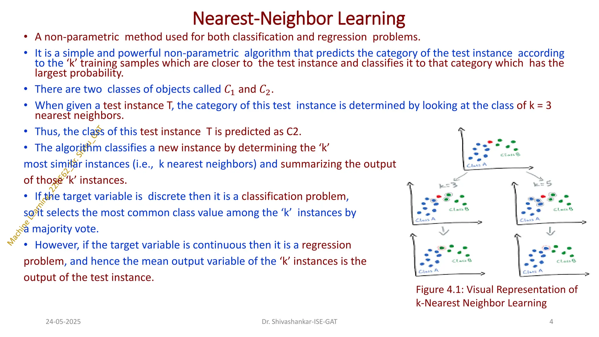
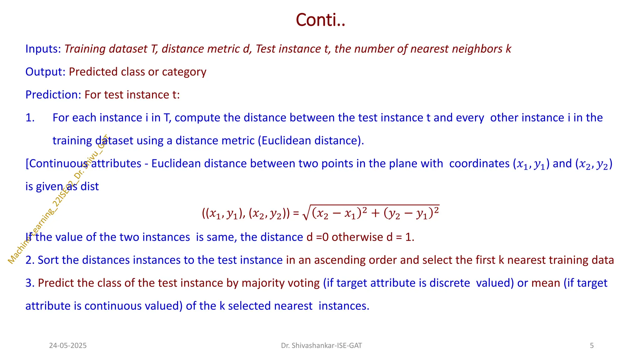
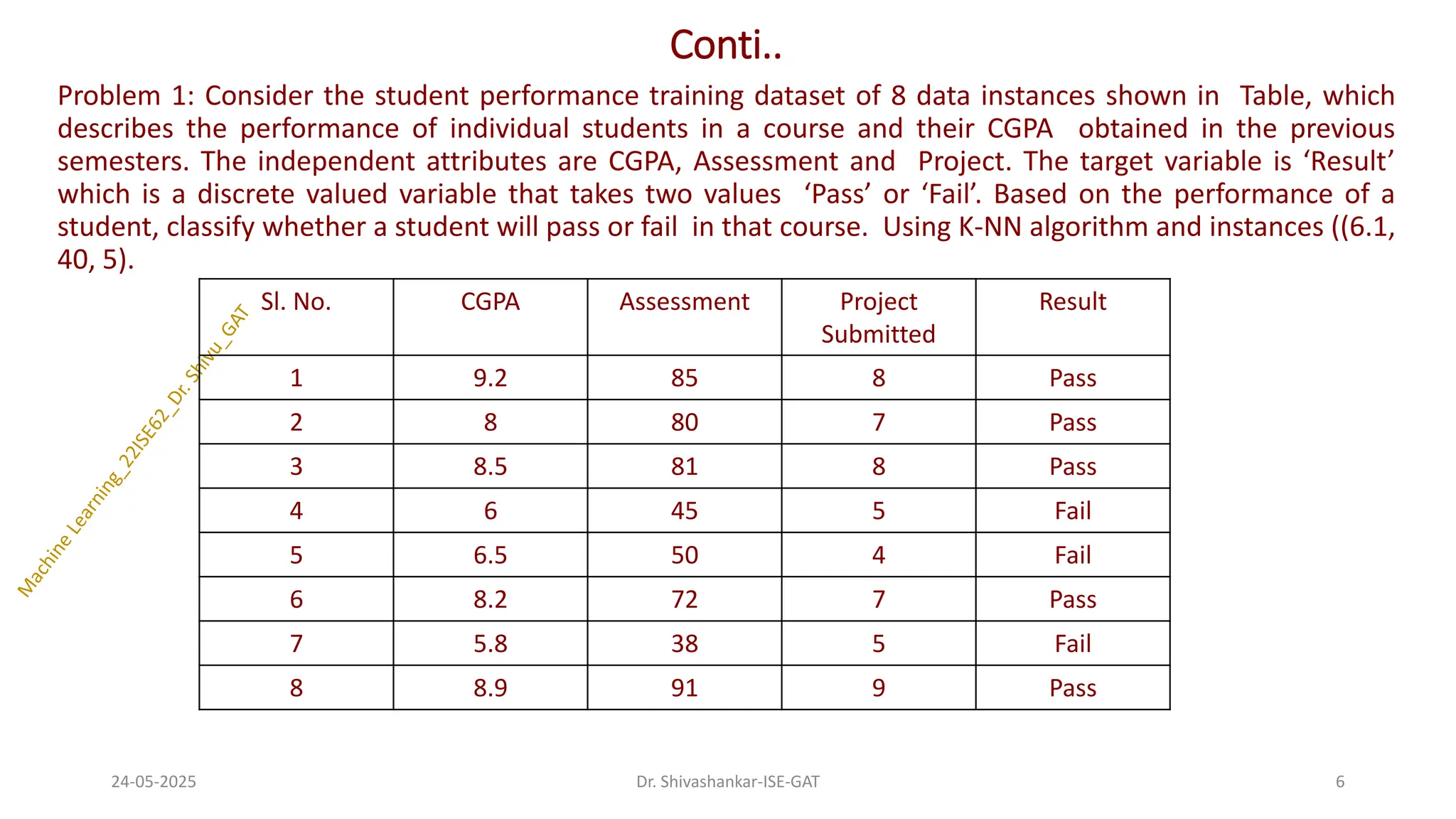
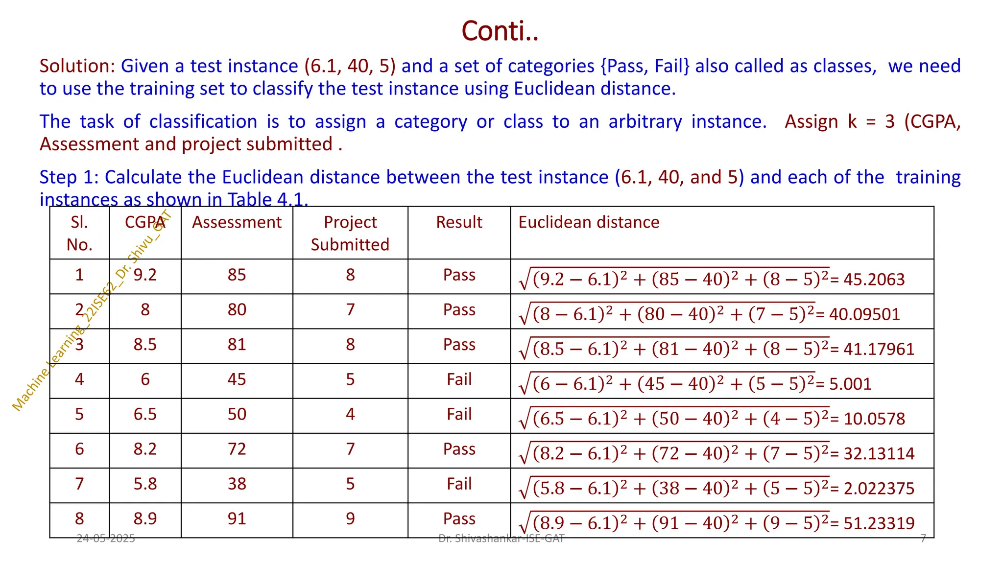
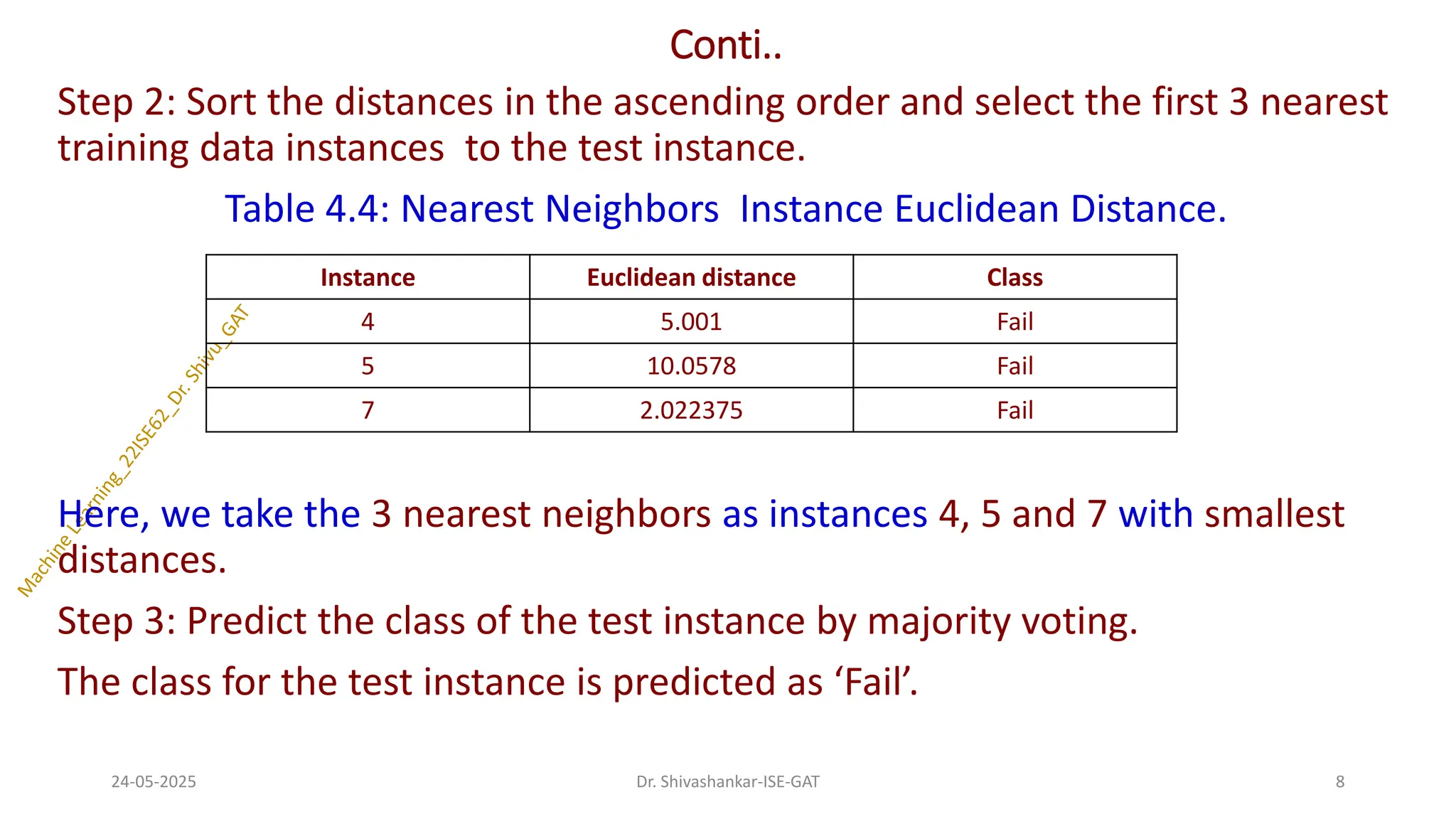
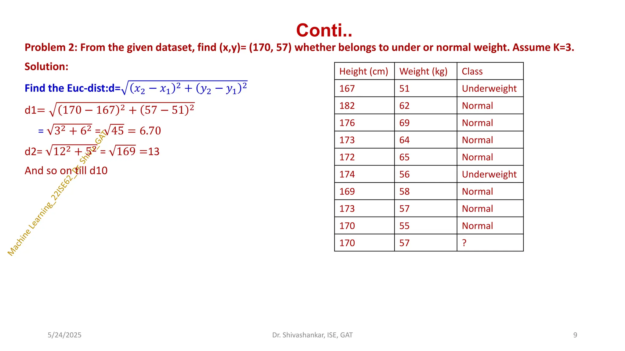
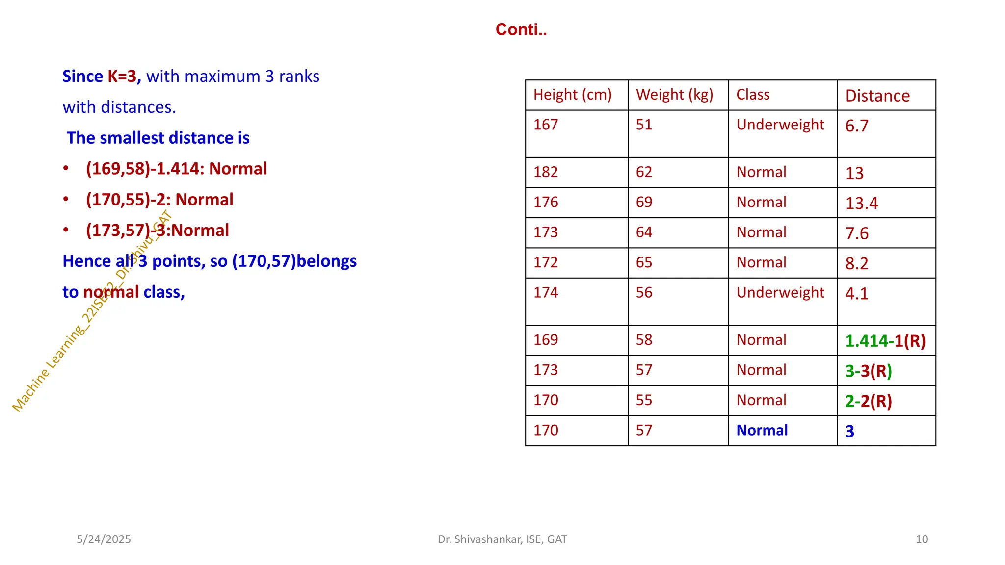
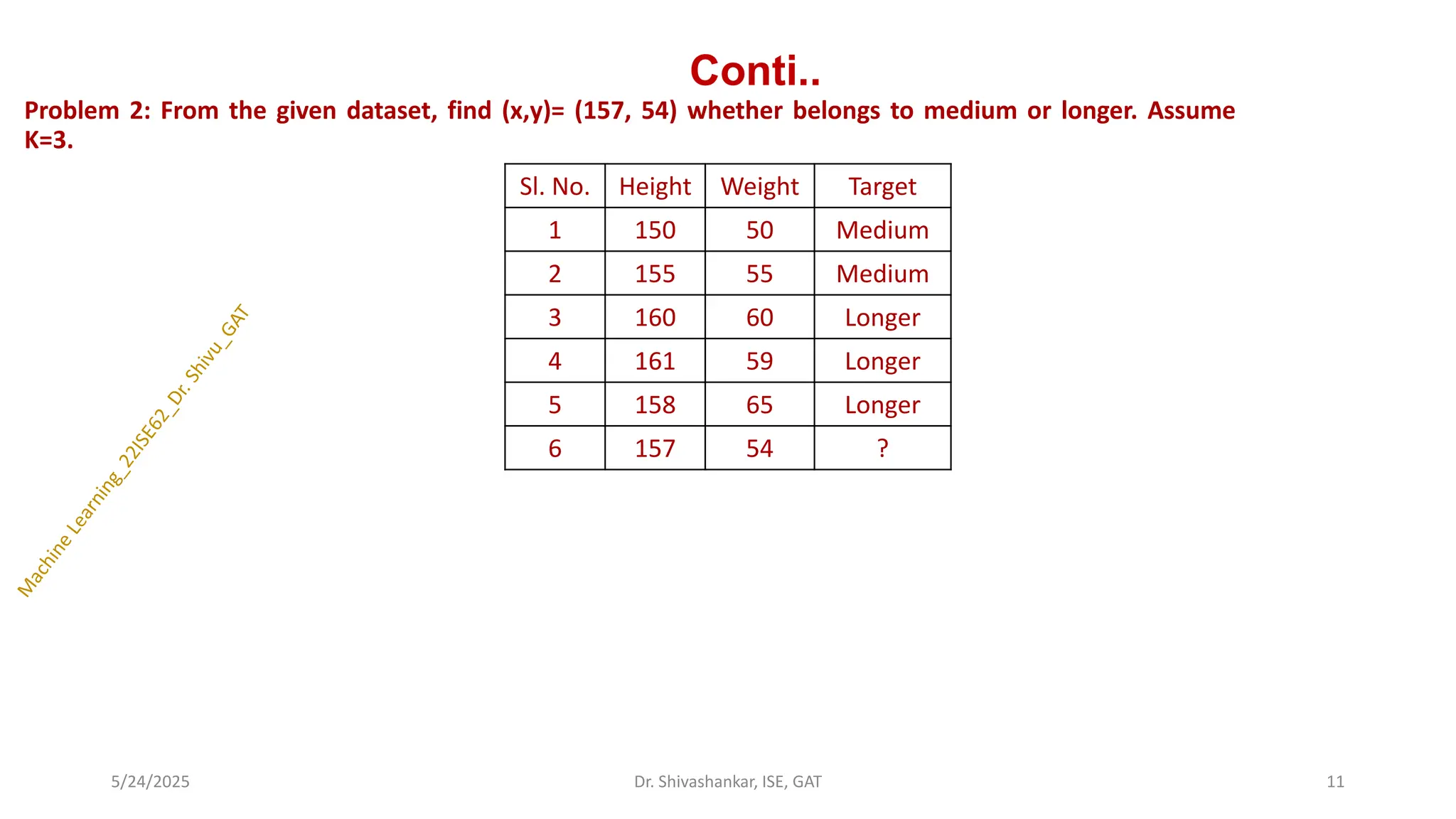
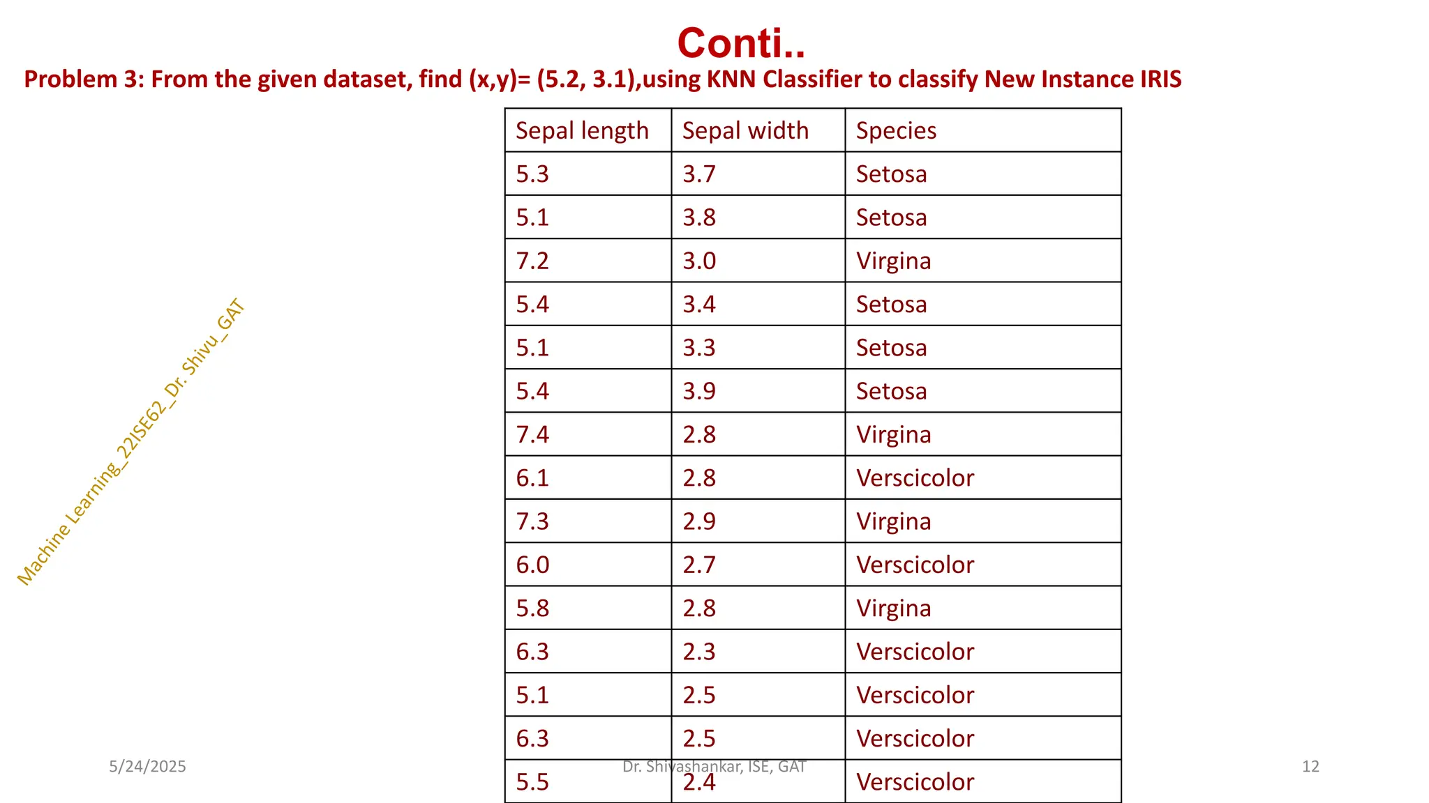
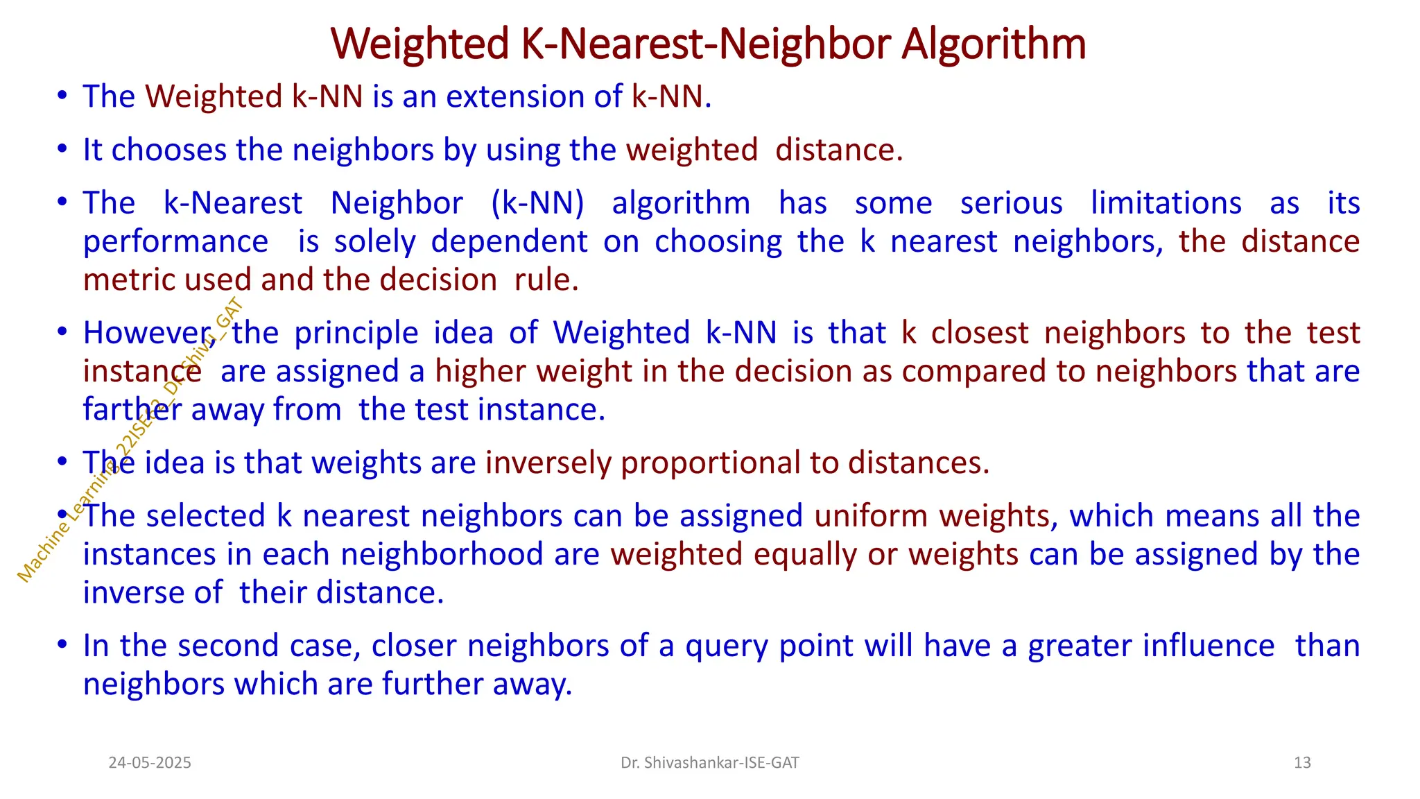
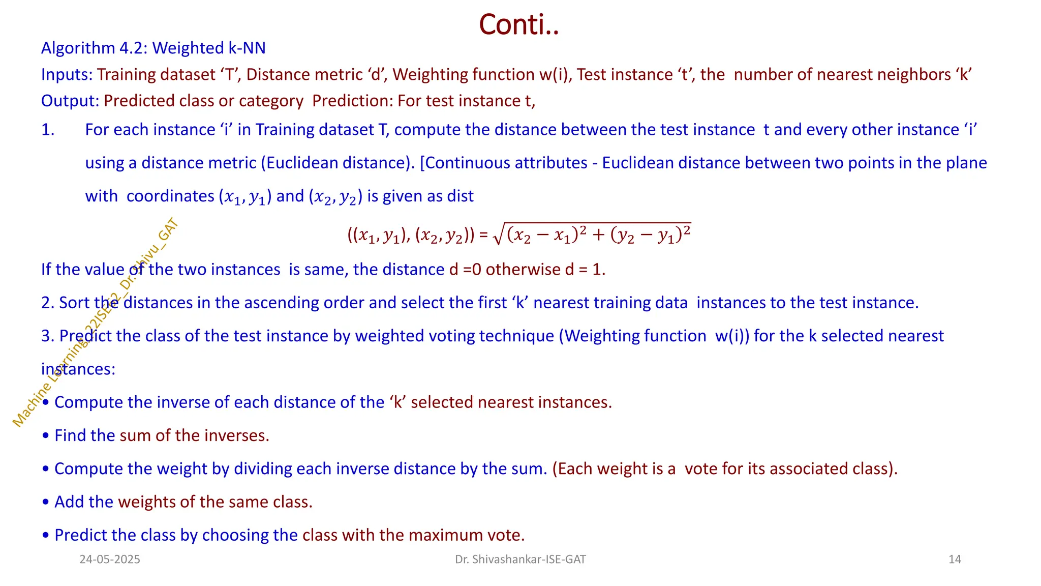
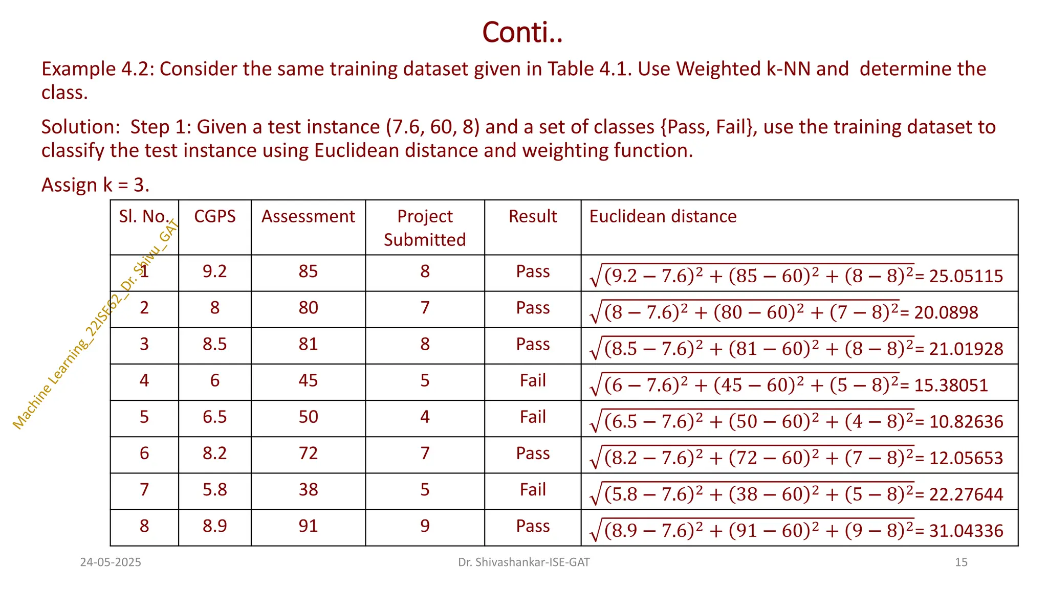
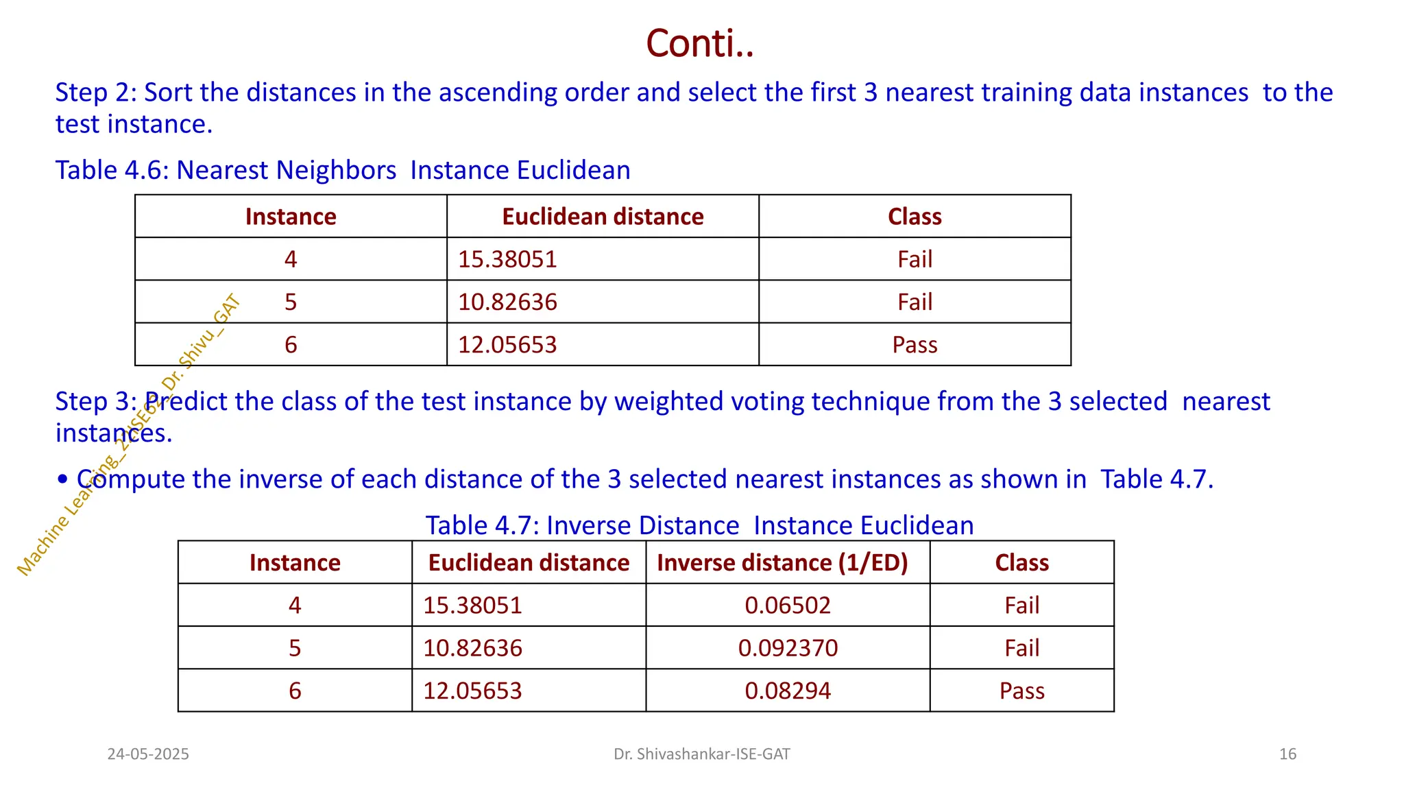
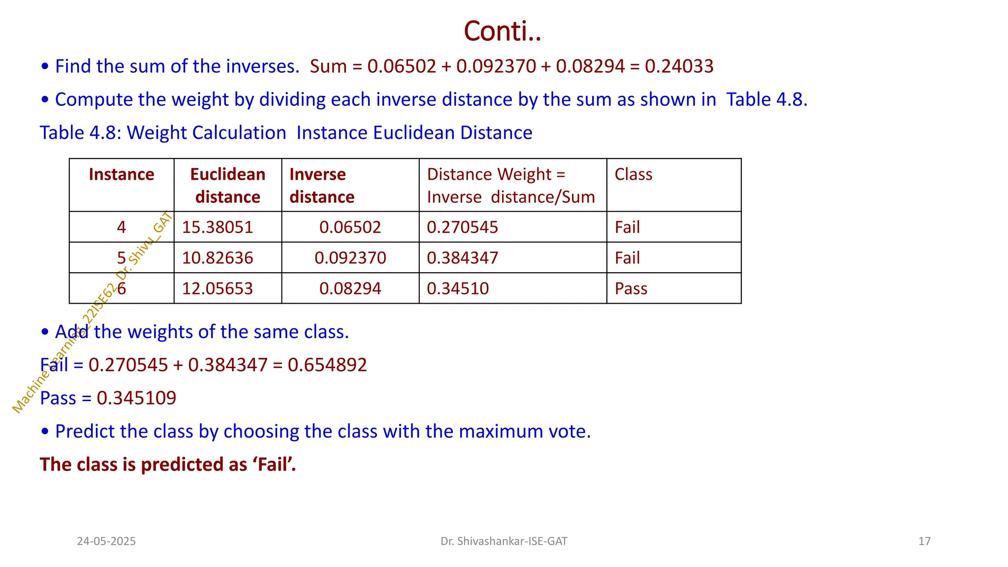
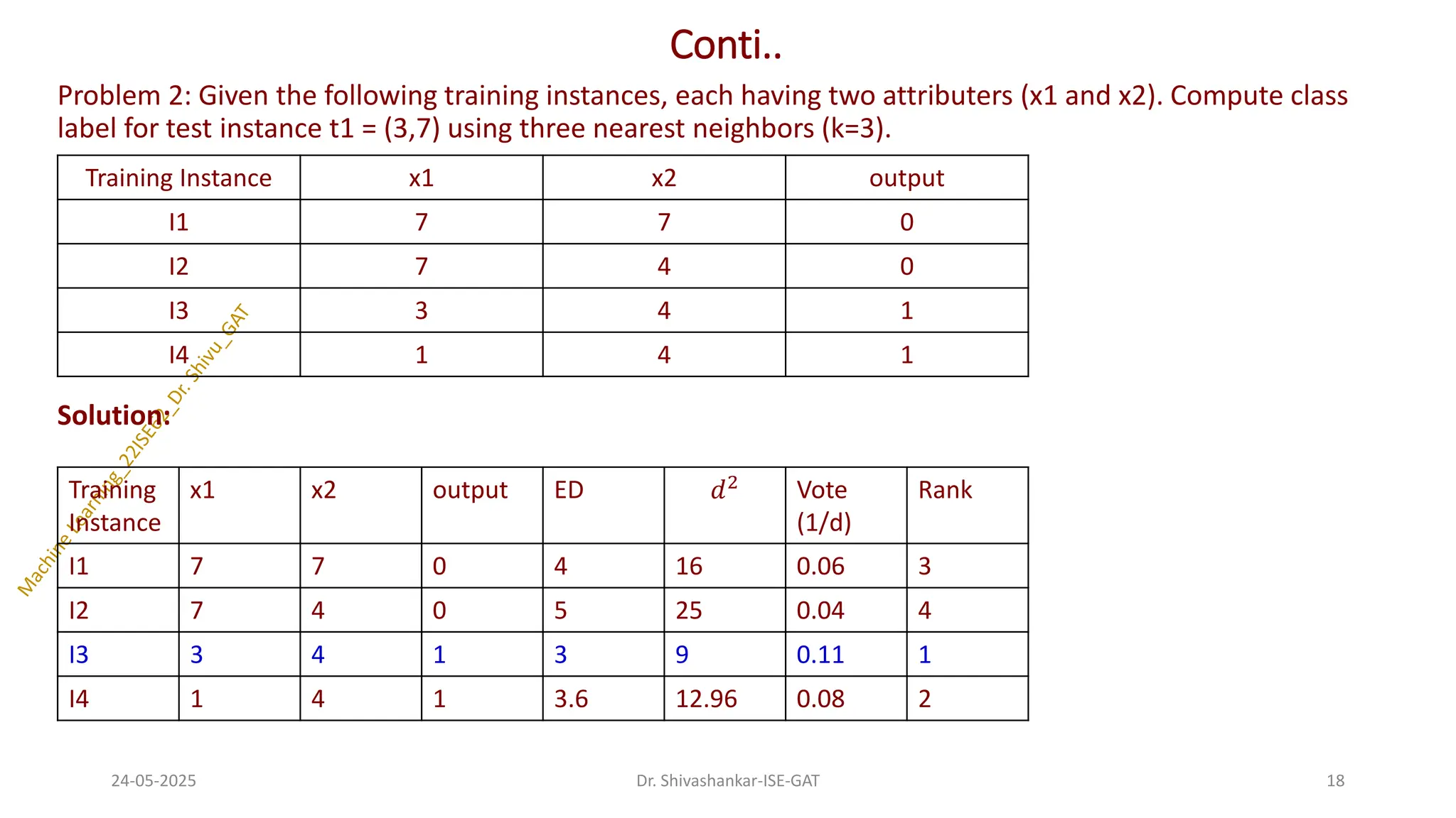
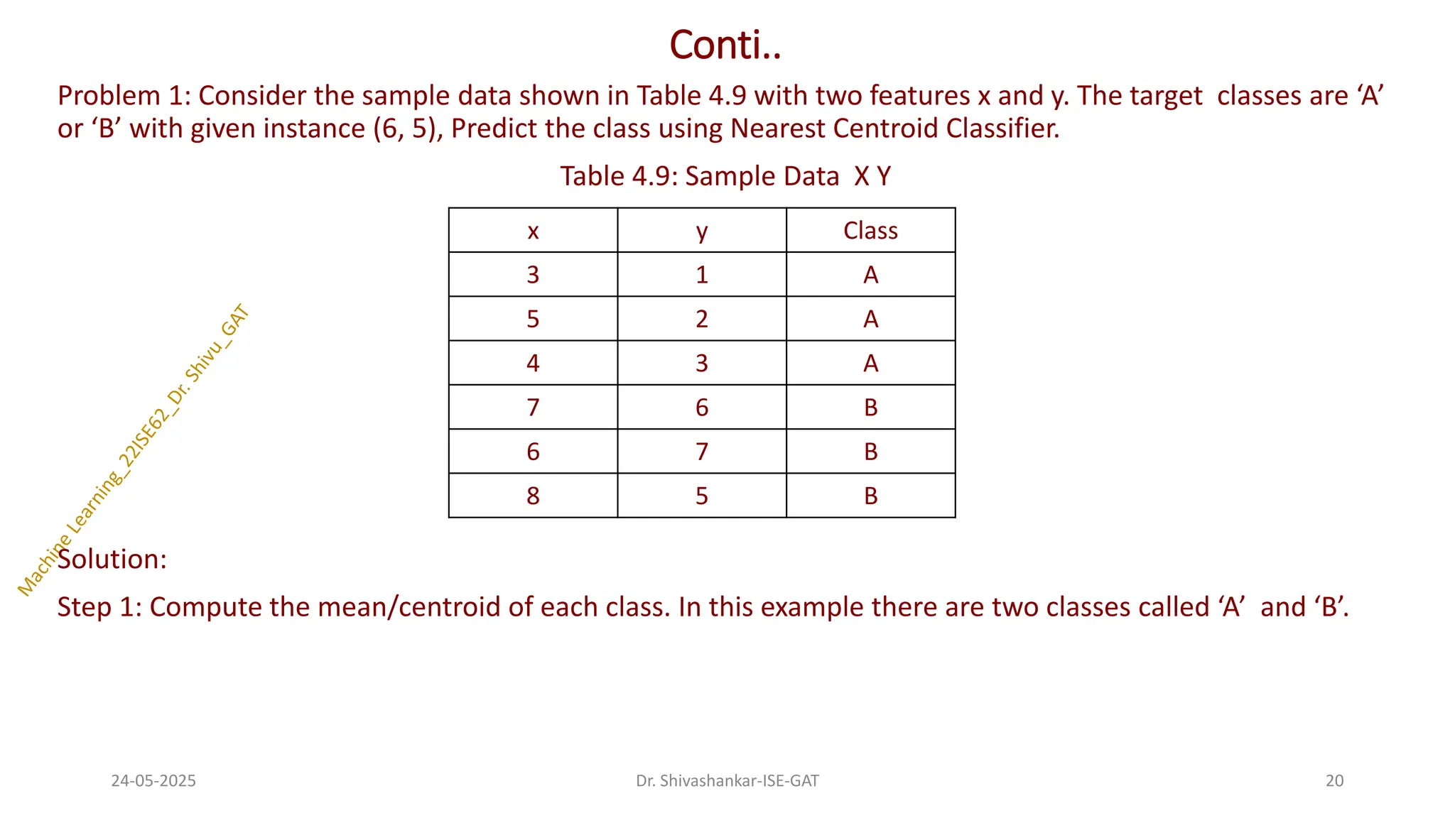
![Conti..
Centroid of class ‘A’ = (3 + 5 + 4, 1 + 2 + 3)/3 = (12, 6)/3 = (4, 2)
Centroid of class ‘B’ = (7 + 6 + 8, 6 + 7 + 5)/3 = (21, 18)/3 = (7, 6)
Now given a test instance (6, 5), we can predict the class.
Step 2: Calculate the Euclidean distance between test instance (6, 5) and each of the centroid.
Euc_Dist[(6, 5); (4, 2)] = 6 − 4 2 + 5 − 2 2= 3.6
Euc_Dist[(6, 5); (7, 6)] = 6 − 7 2 + 5 − 6 2= 1.414
The test instance has smaller distance to class B. Hence, the class of this test instance is predicted as ‘B’.
24-05-2025 21
Dr. Shivashankar-ISE-GAT](https://image.slidesharecdn.com/machinelearning-module3-250524092052-1361b02d/75/Dr-Shivu__Machine-Learning-Module-3-pdf-21-2048.jpg)
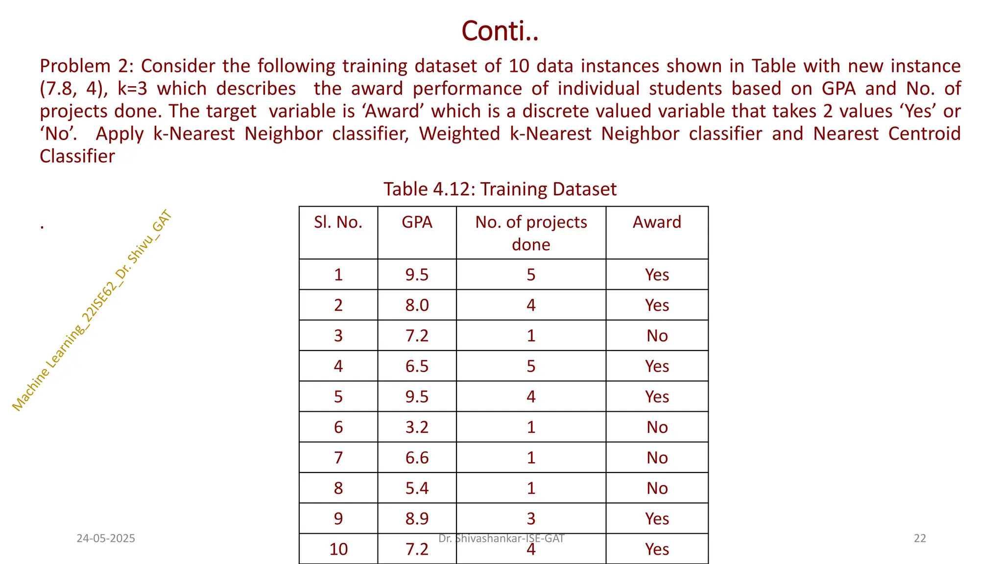
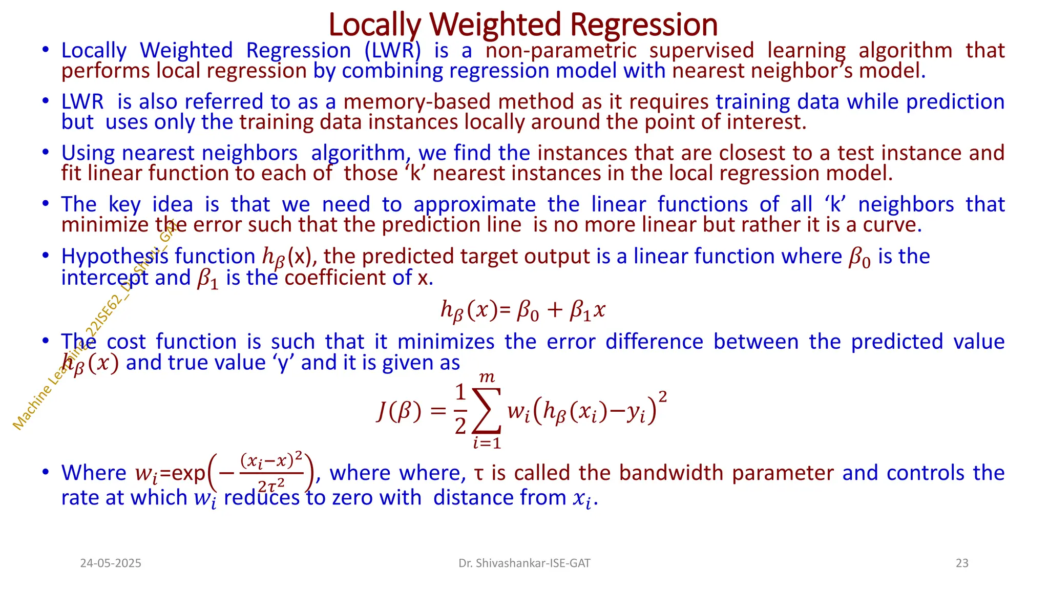
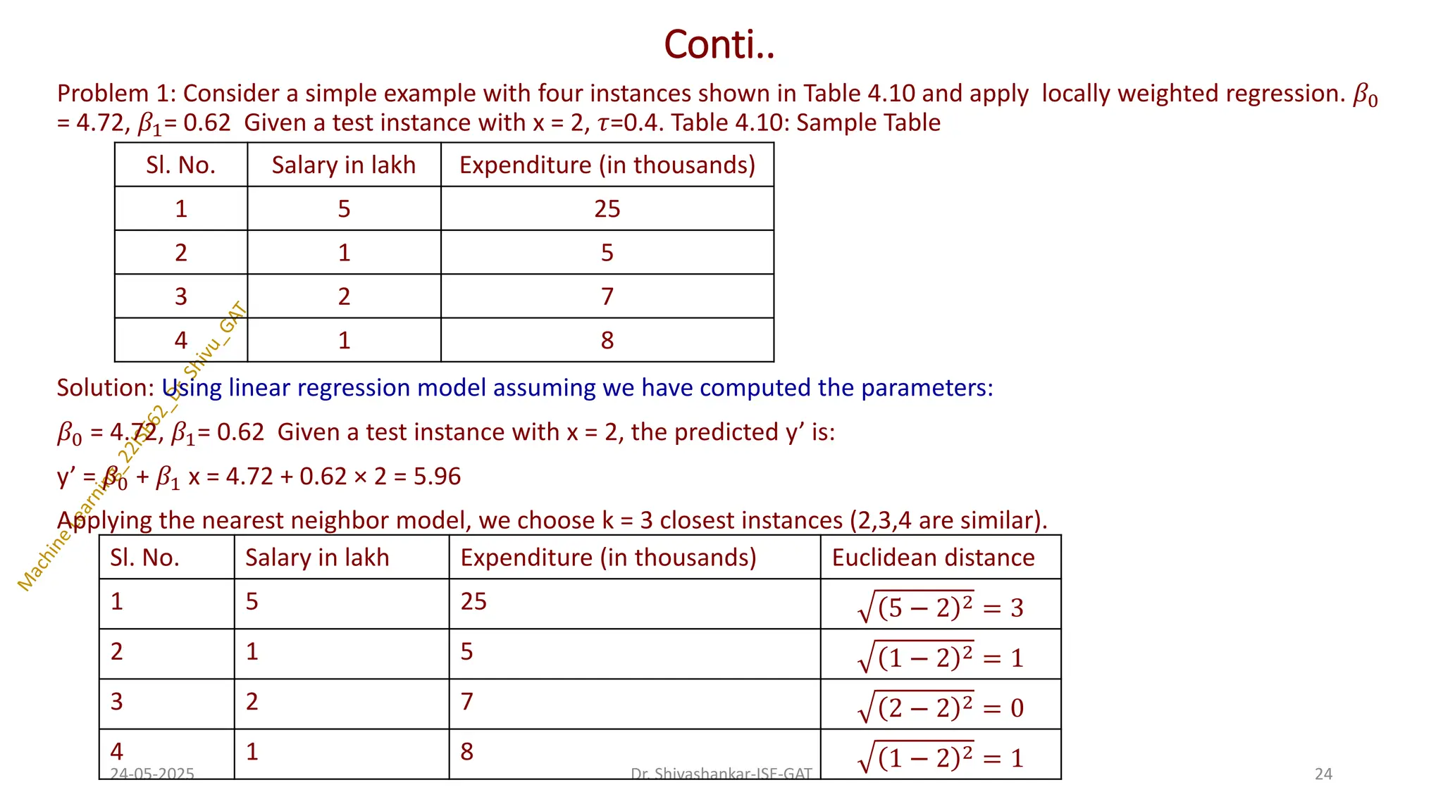
![Conti..
Instances 2, 3 and 4 are closer with smaller distances. The mean value = (5 + 7 + 8)/3 =
20/3 = 6.67. Compute the weights for the closest instances, using the Gaussian kernel
𝑤𝑖=exp −
𝑥𝑖−𝑥 2
2𝜏2
Weight of Instance 2:
𝑤2=exp −
𝑥2−𝑥 2
2𝜏2 = exp −
1−2 2
2𝑥0.42 = 𝑒−3.125= 0.043
Weight of Instance 3:
𝑤3=exp −
𝑥3−𝑥 2
2𝜏2 = exp −
2−2 2
2𝑥0.42 = 𝑒0= 1
Weight of Instance 4:
𝑤4=exp −
𝑥4−𝑥 2
2𝜏2 = exp −
1−2 2
2𝑥0.42 = 𝑒−3.125= 0.043
𝑒0
= 1 [𝑤3 is closer hence gets a higher weight value]
24-05-2025 25
Dr. Shivashankar-ISE-GAT](https://image.slidesharecdn.com/machinelearning-module3-250524092052-1361b02d/75/Dr-Shivu__Machine-Learning-Module-3-pdf-25-2048.jpg)
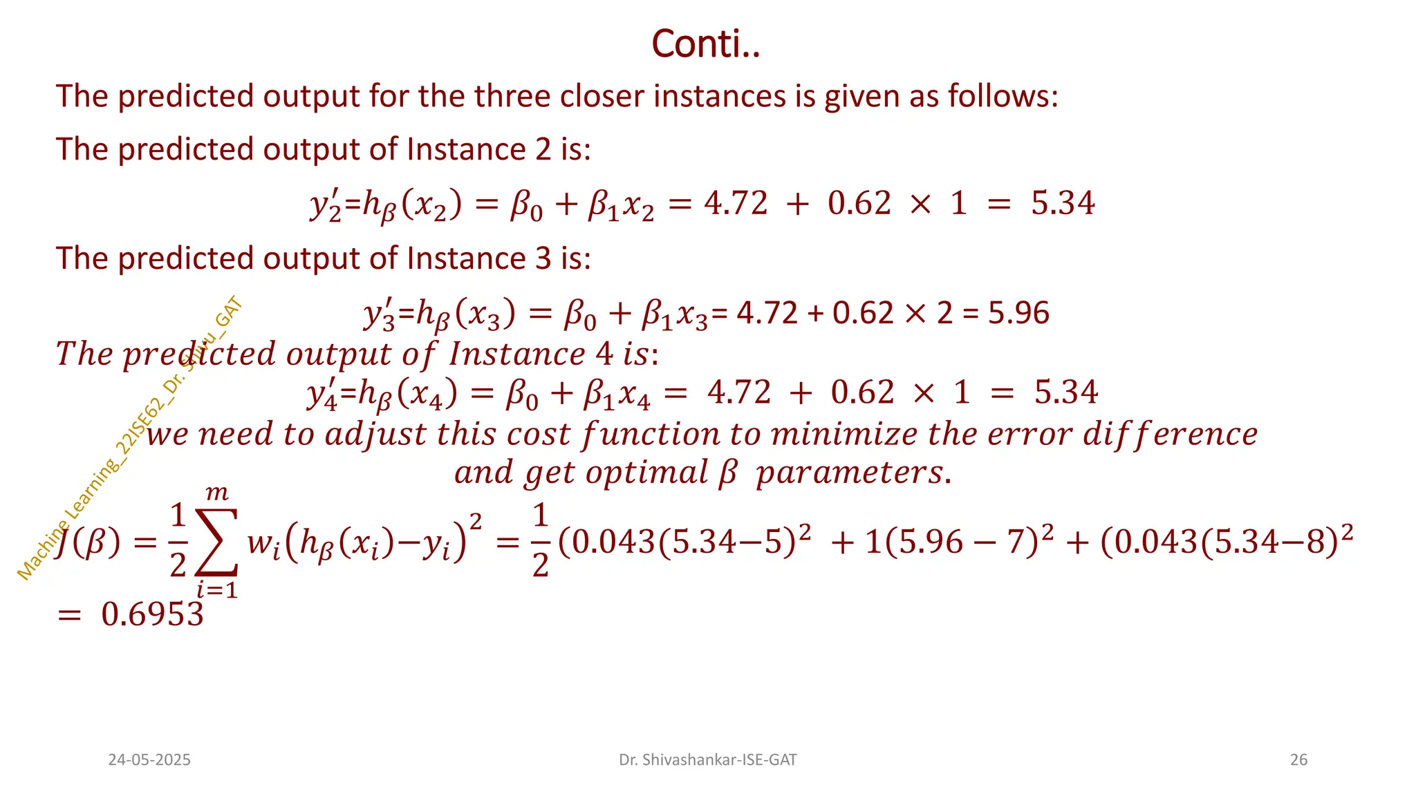
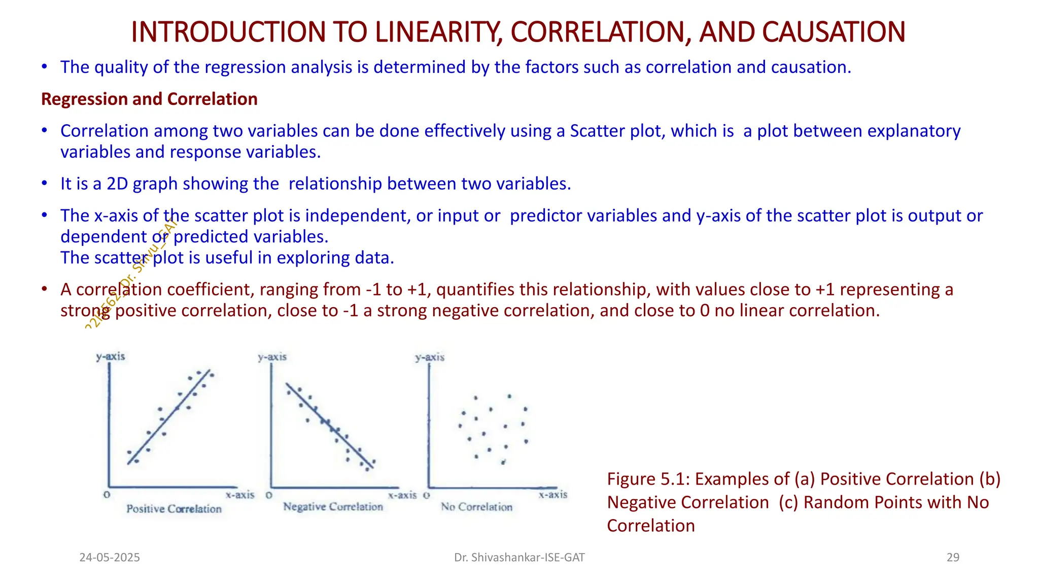
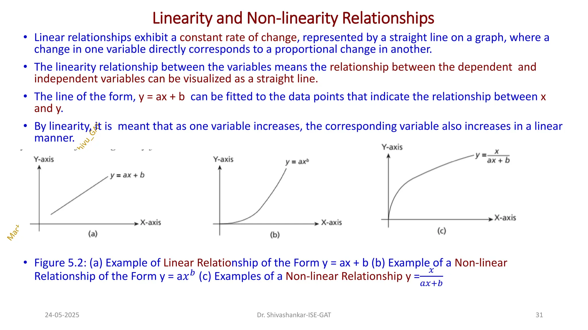
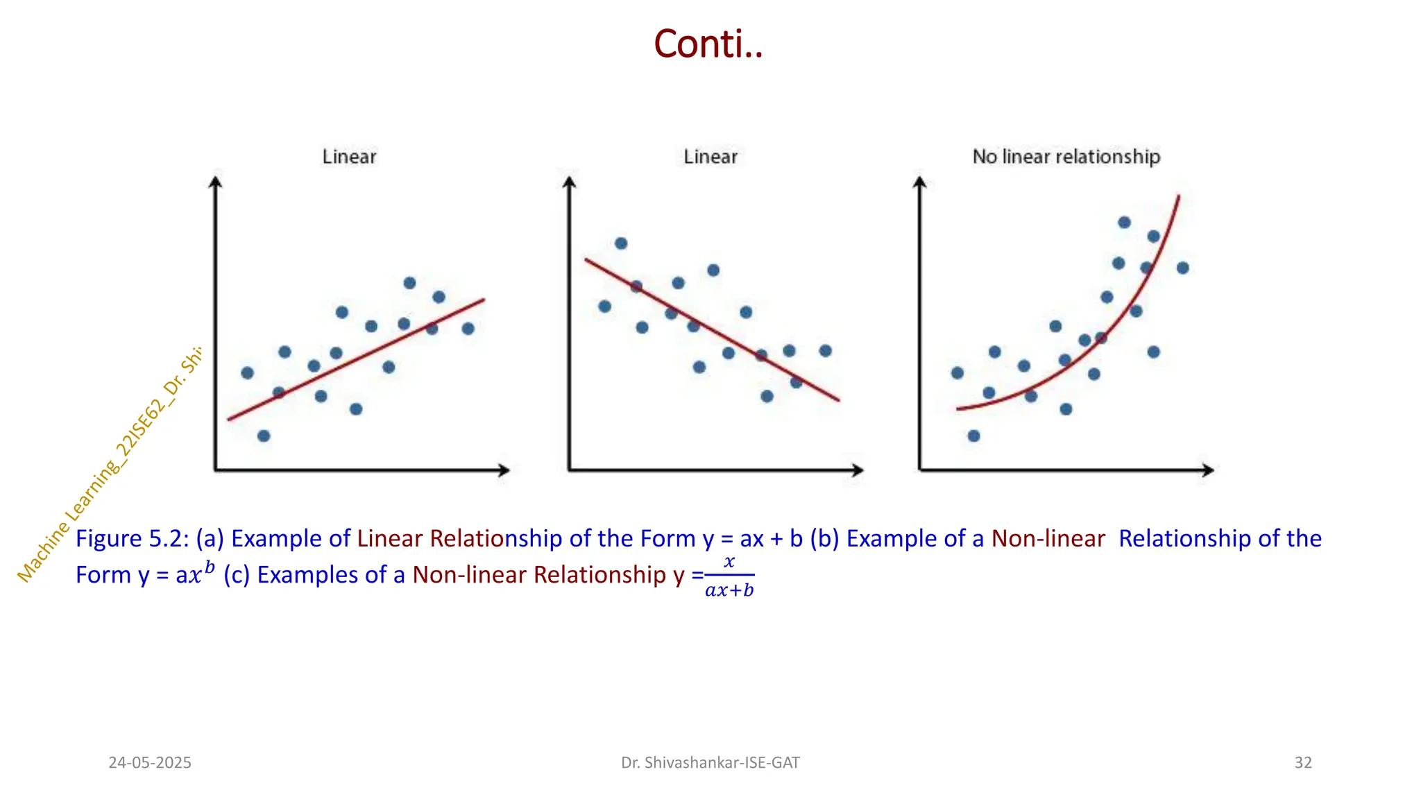
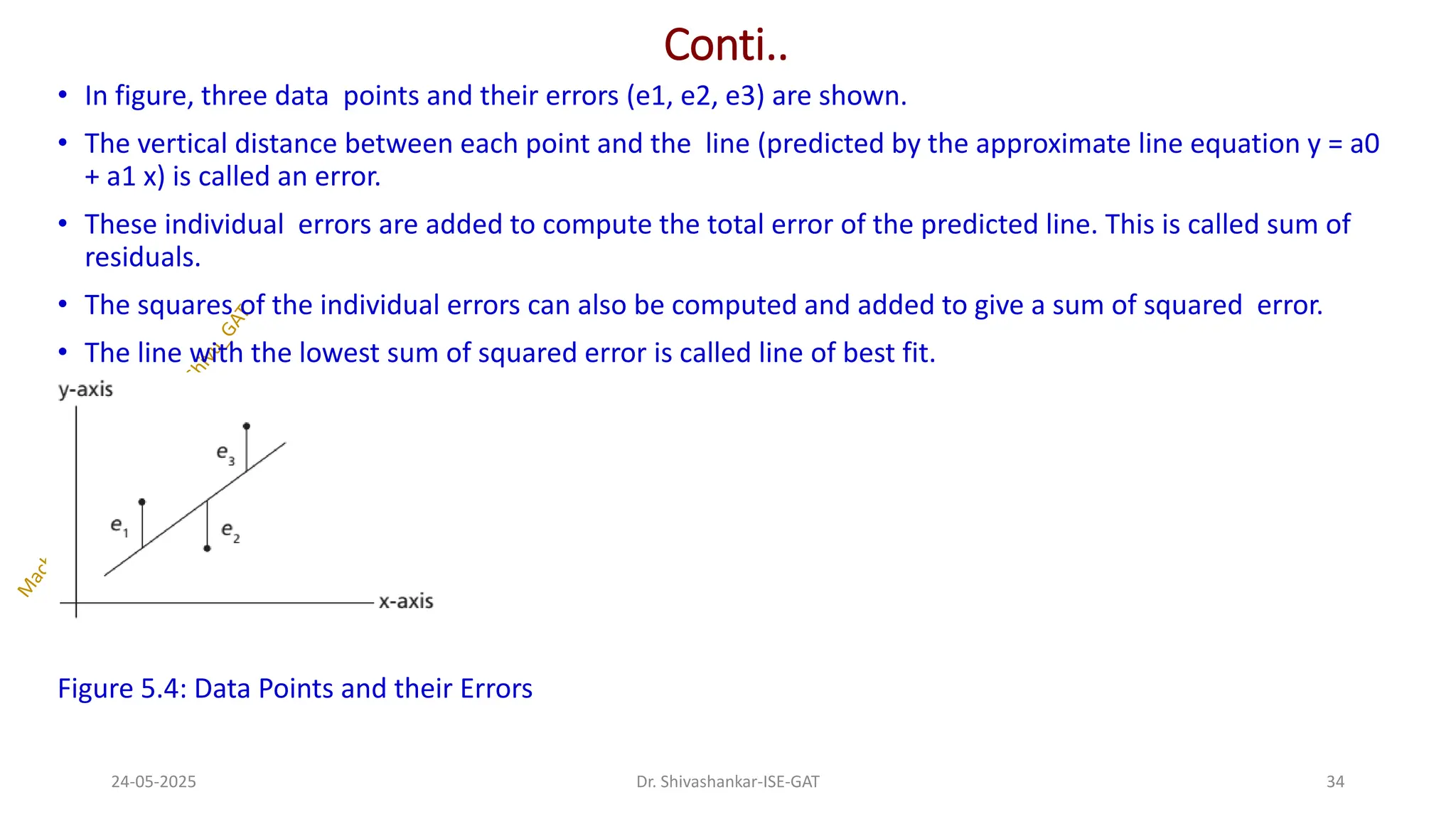
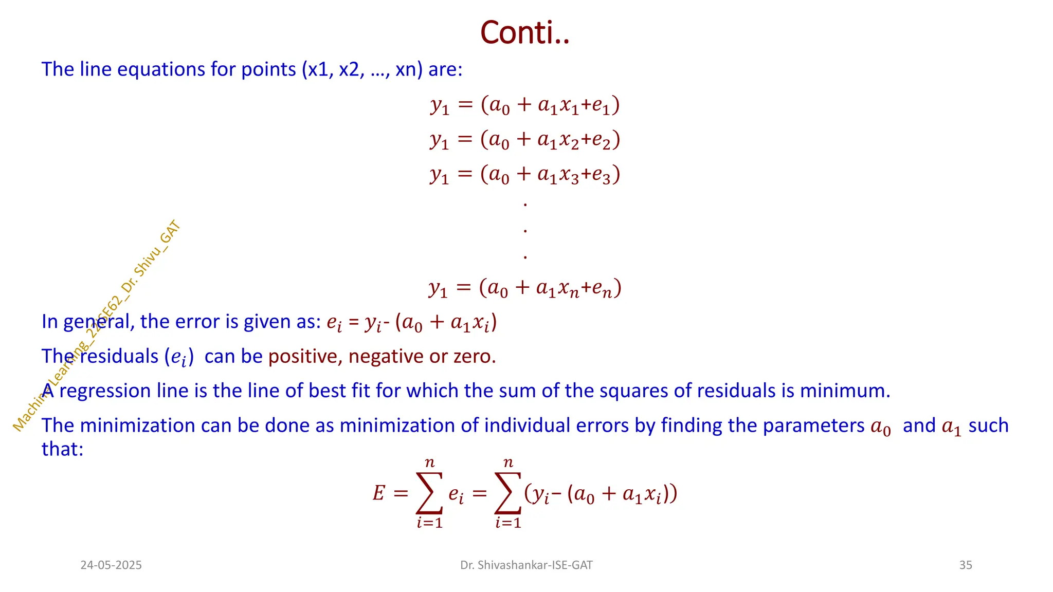
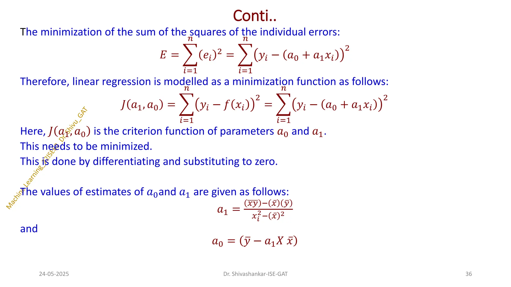
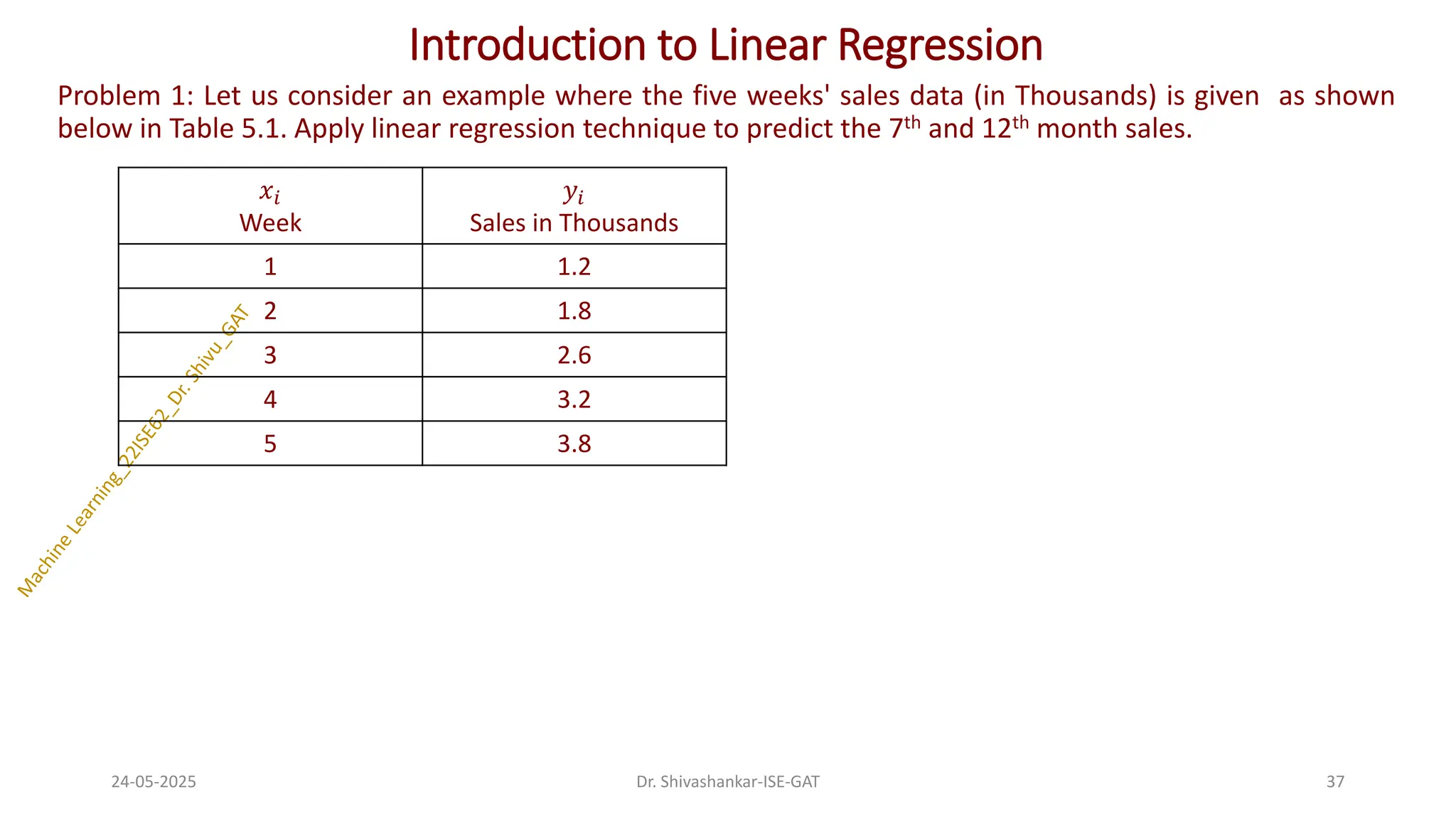
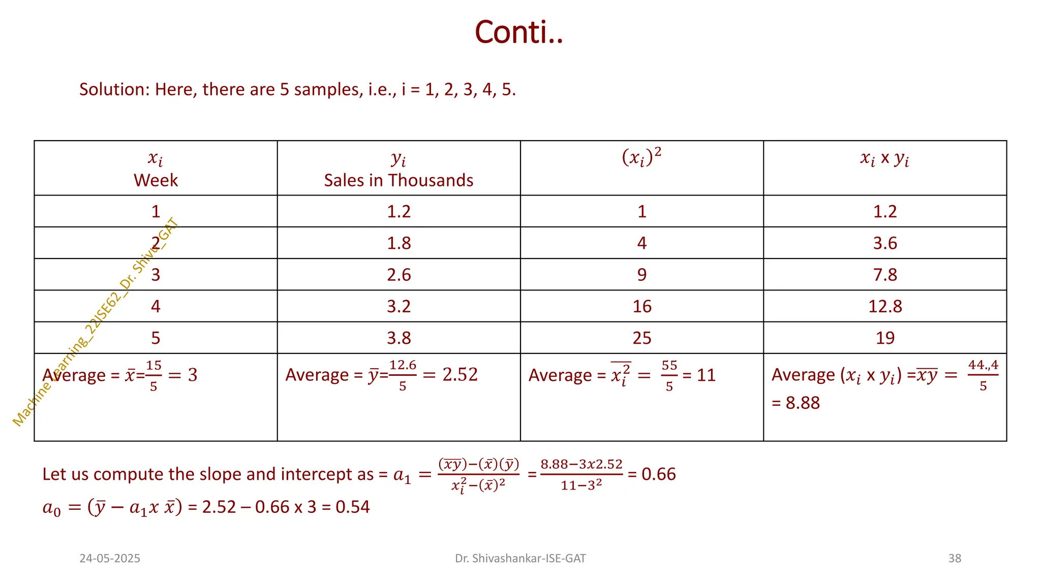
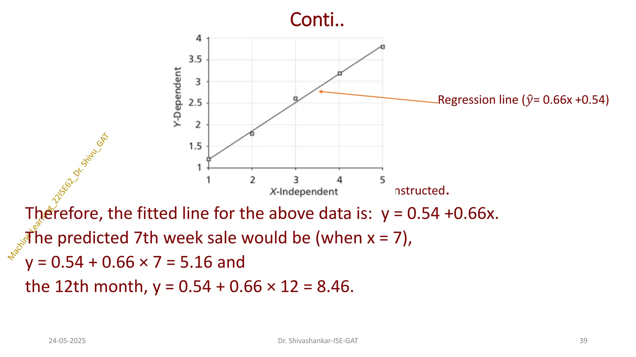
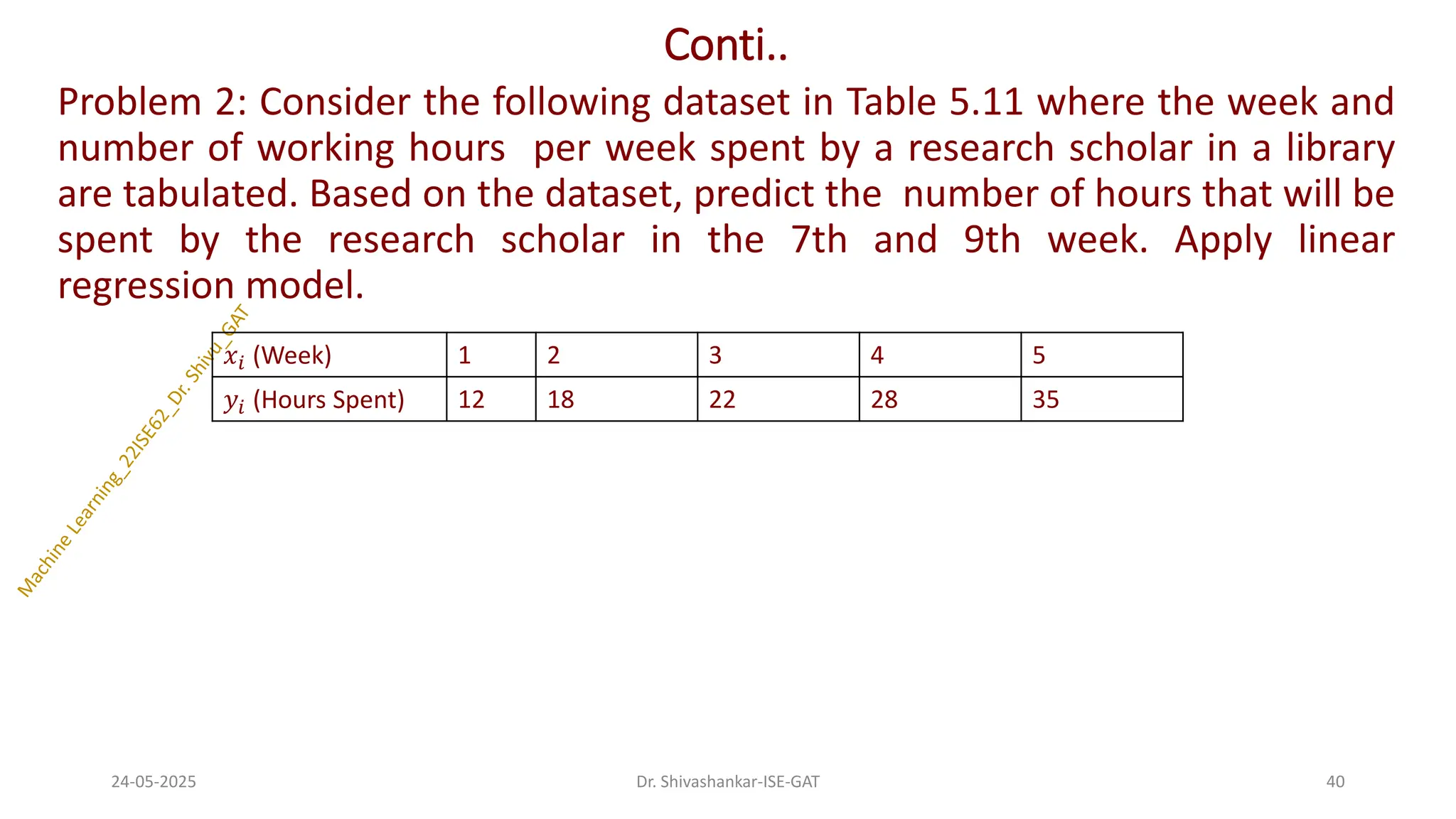
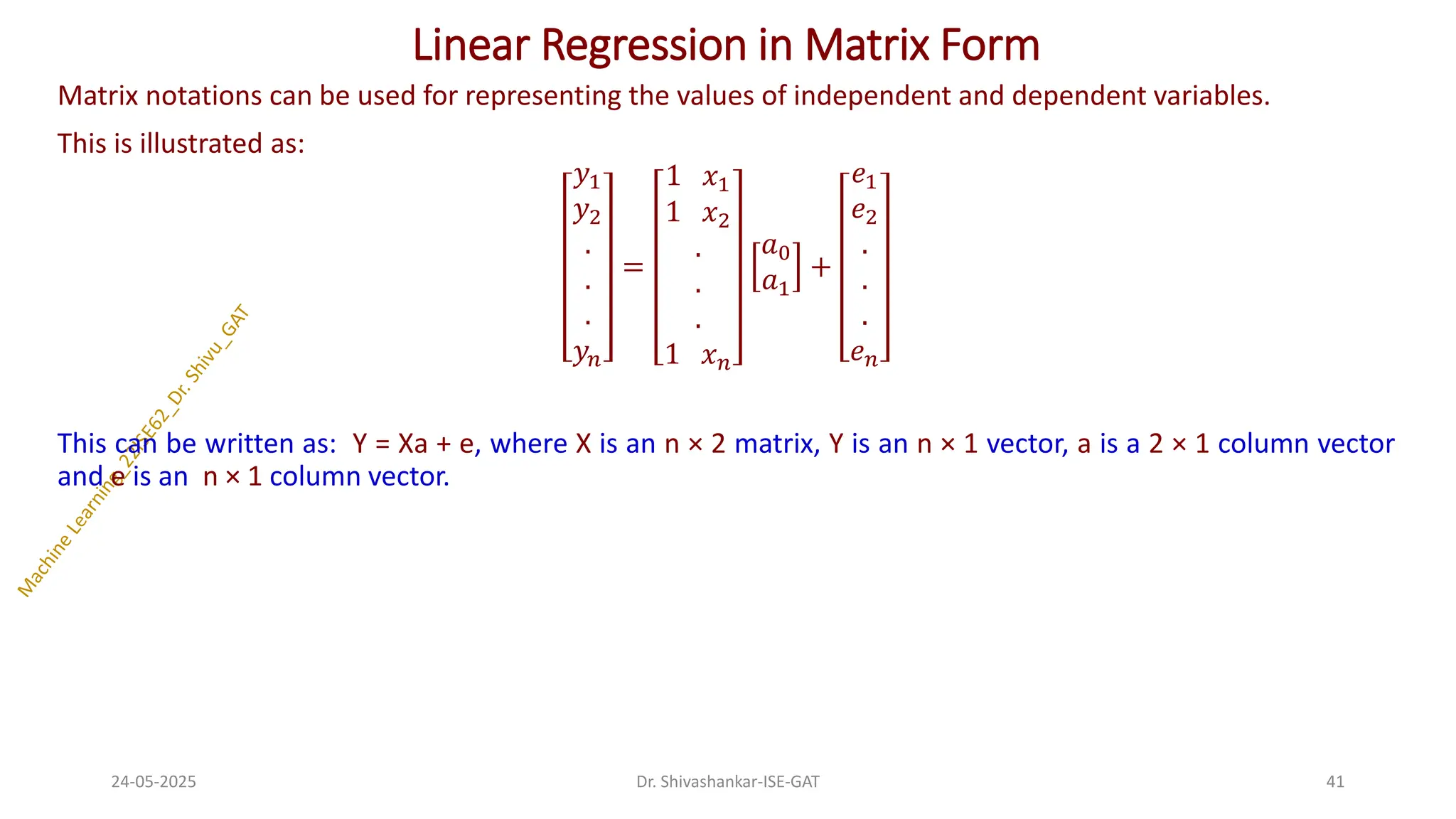
![Conti..
Problem 1: Find linear regression of the data of week and product sales (in Thousands). Use linear regression
in matrix form.
Table 5.3: Sample Data for Regression
Solution: Solution: The dependent variable X is be given as: 𝑥𝑇 = [1 2 3 4]
And the independent variable is given as follows: 𝑦𝑇 = [1 3 4 8]
The data can be given in matrix form as follows: X
1 1
1 2
1 3
1 4
and Y=
1
3
4
8
24-05-2025 42
Dr. Shivashankar-ISE-GAT
𝑥𝑖
Week
𝑦𝑖
Product Sales in Thousands
1 1
2 3
3 4
4 8](https://image.slidesharecdn.com/machinelearning-module3-250524092052-1361b02d/75/Dr-Shivu__Machine-Learning-Module-3-pdf-42-2048.jpg)
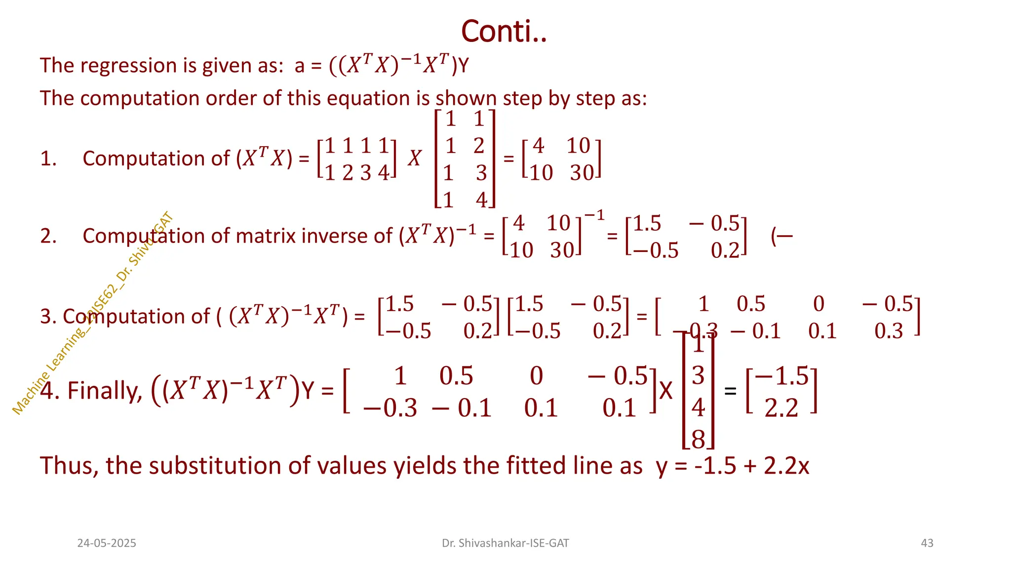
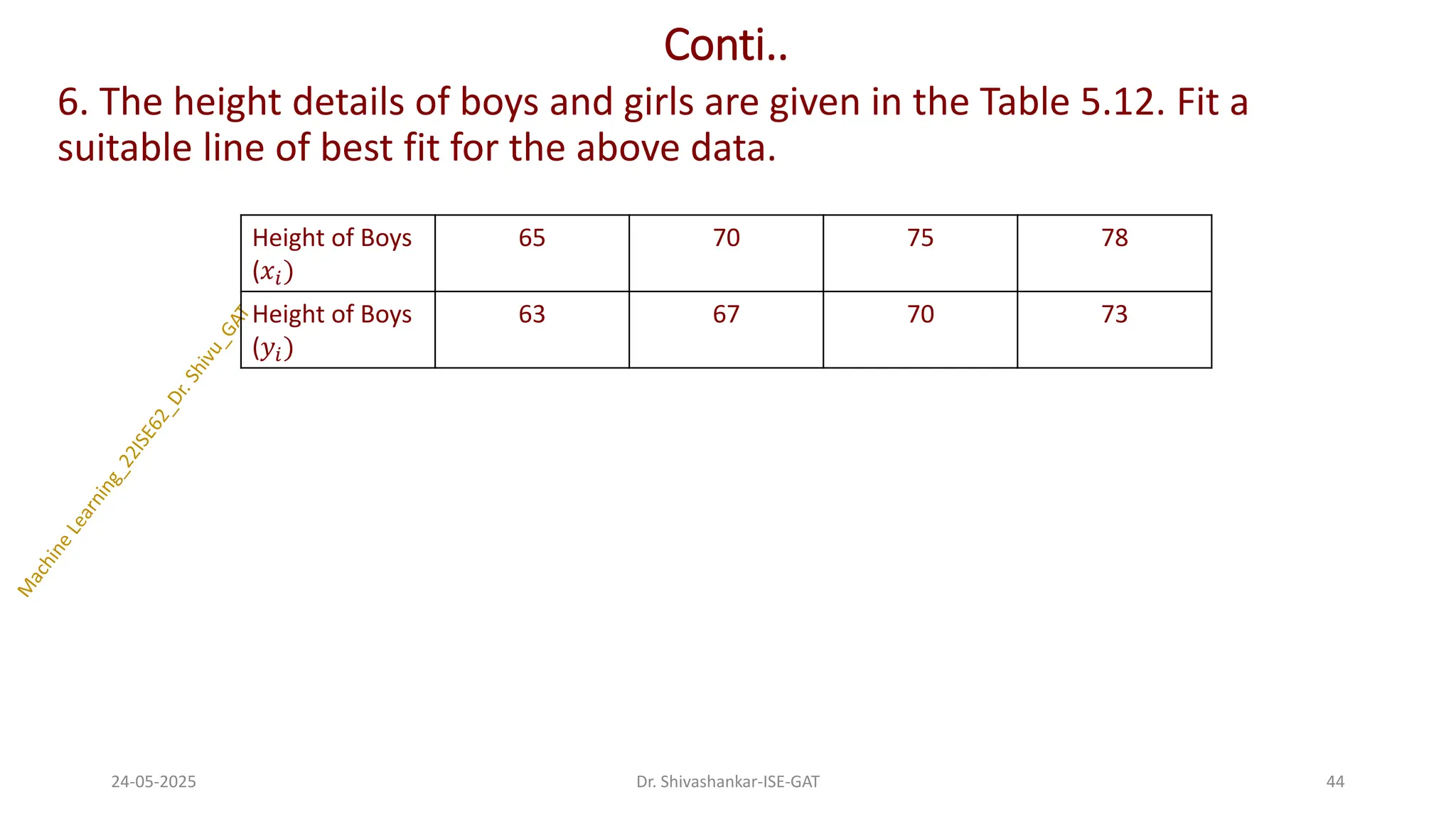
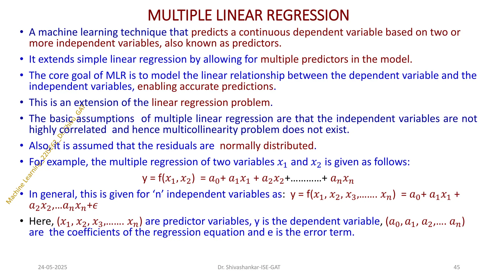
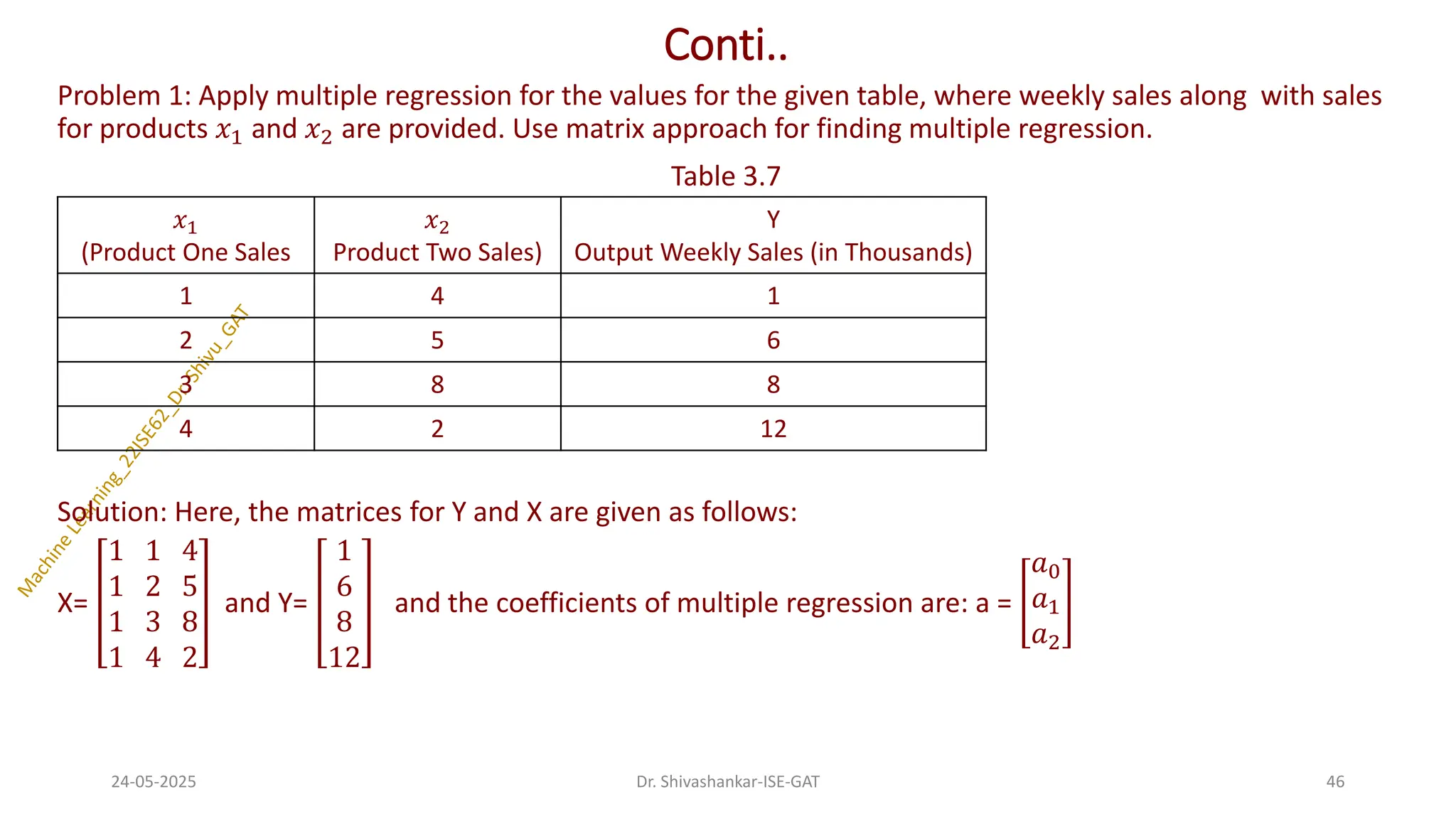
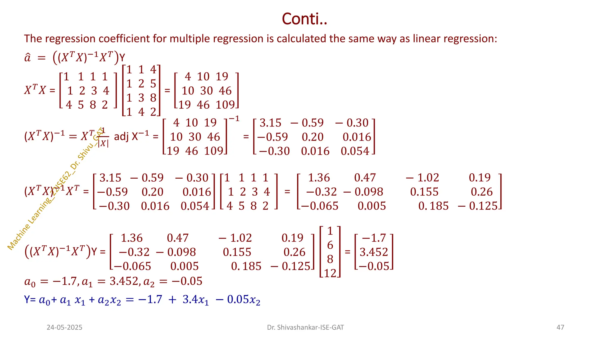
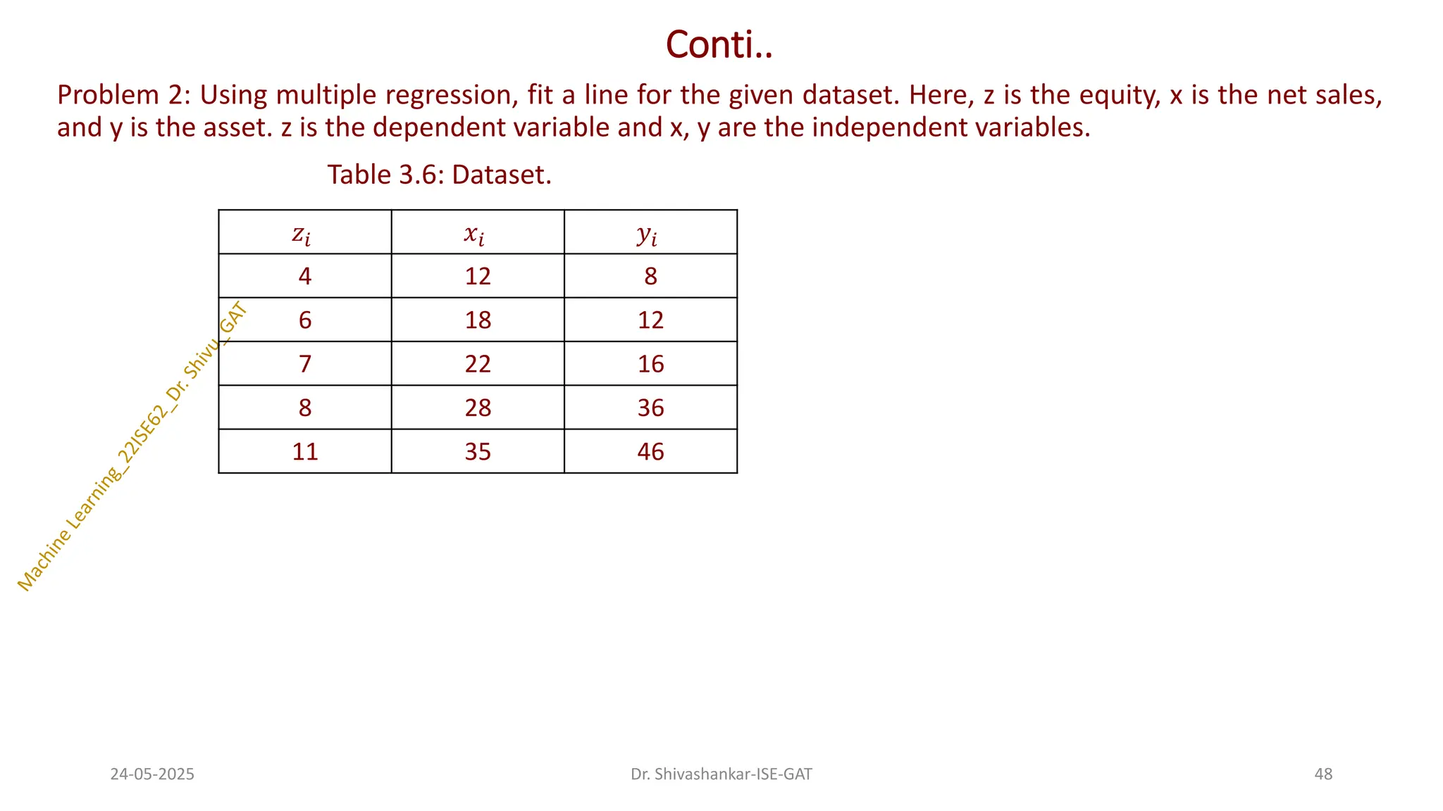
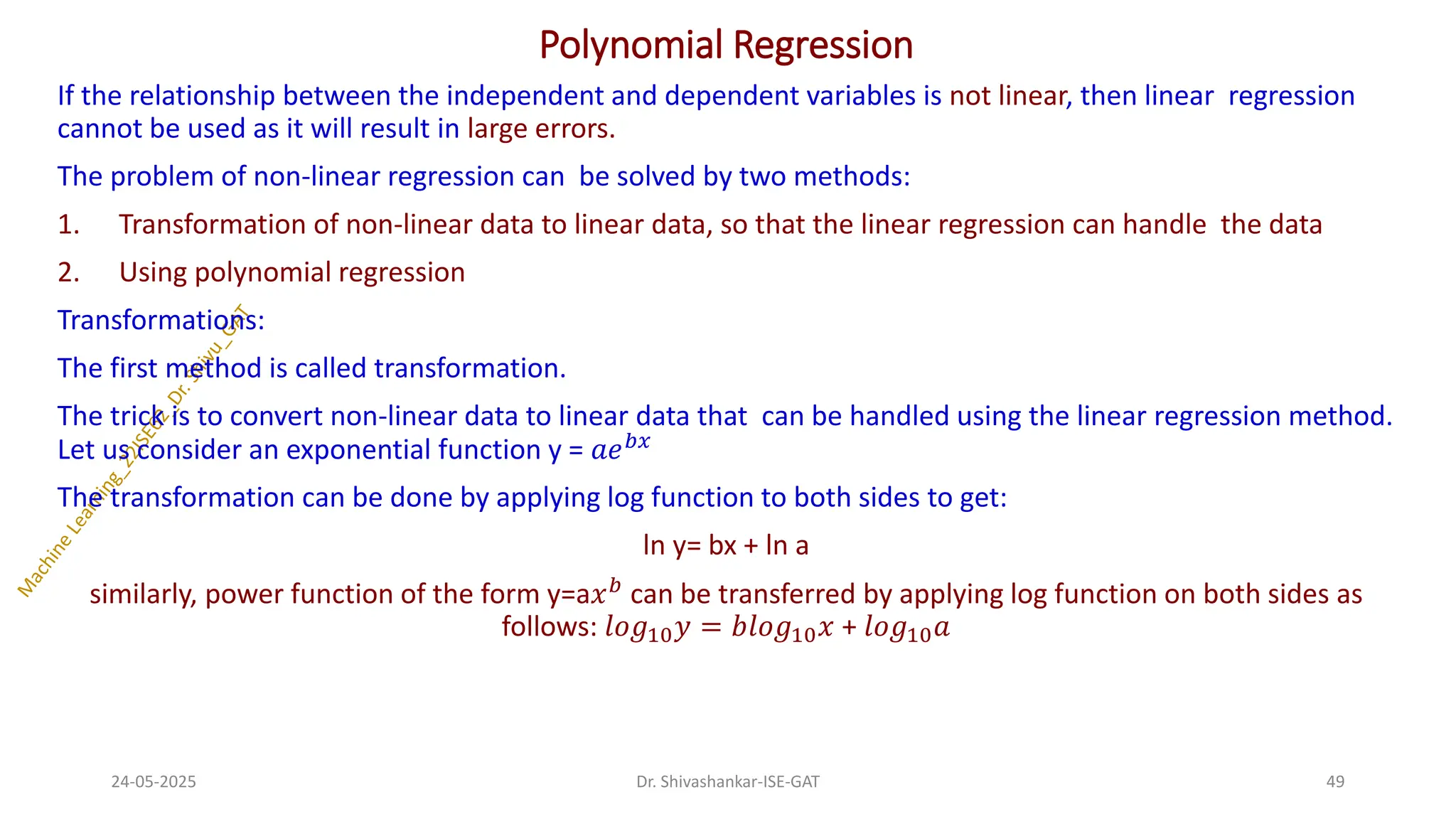
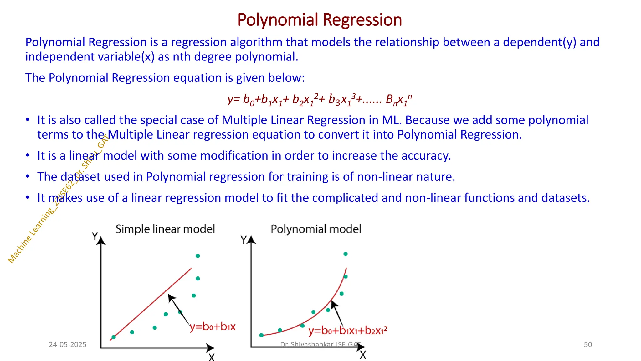
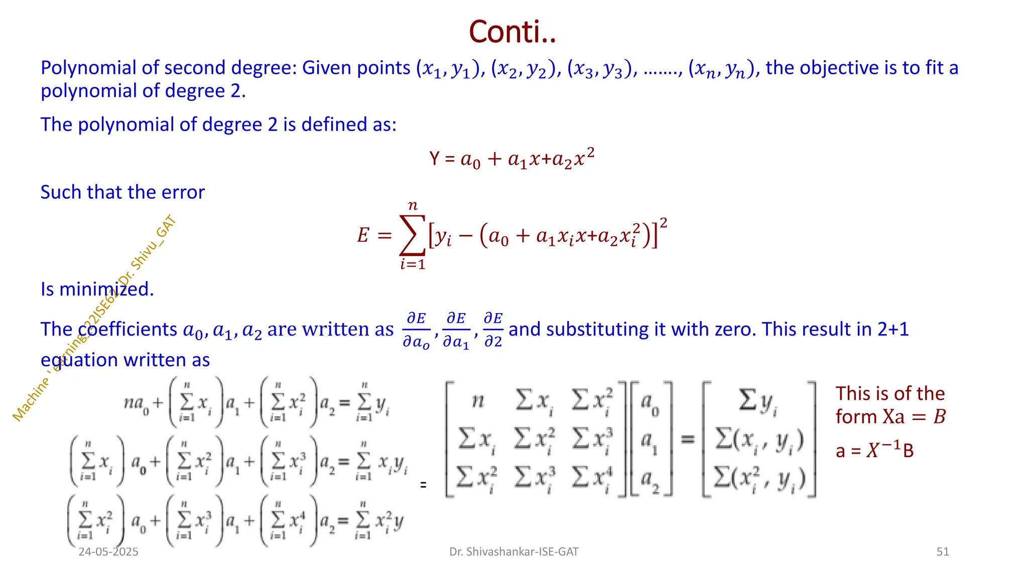
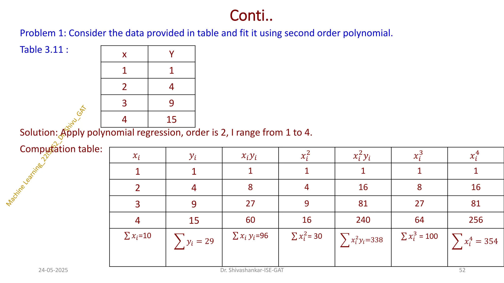
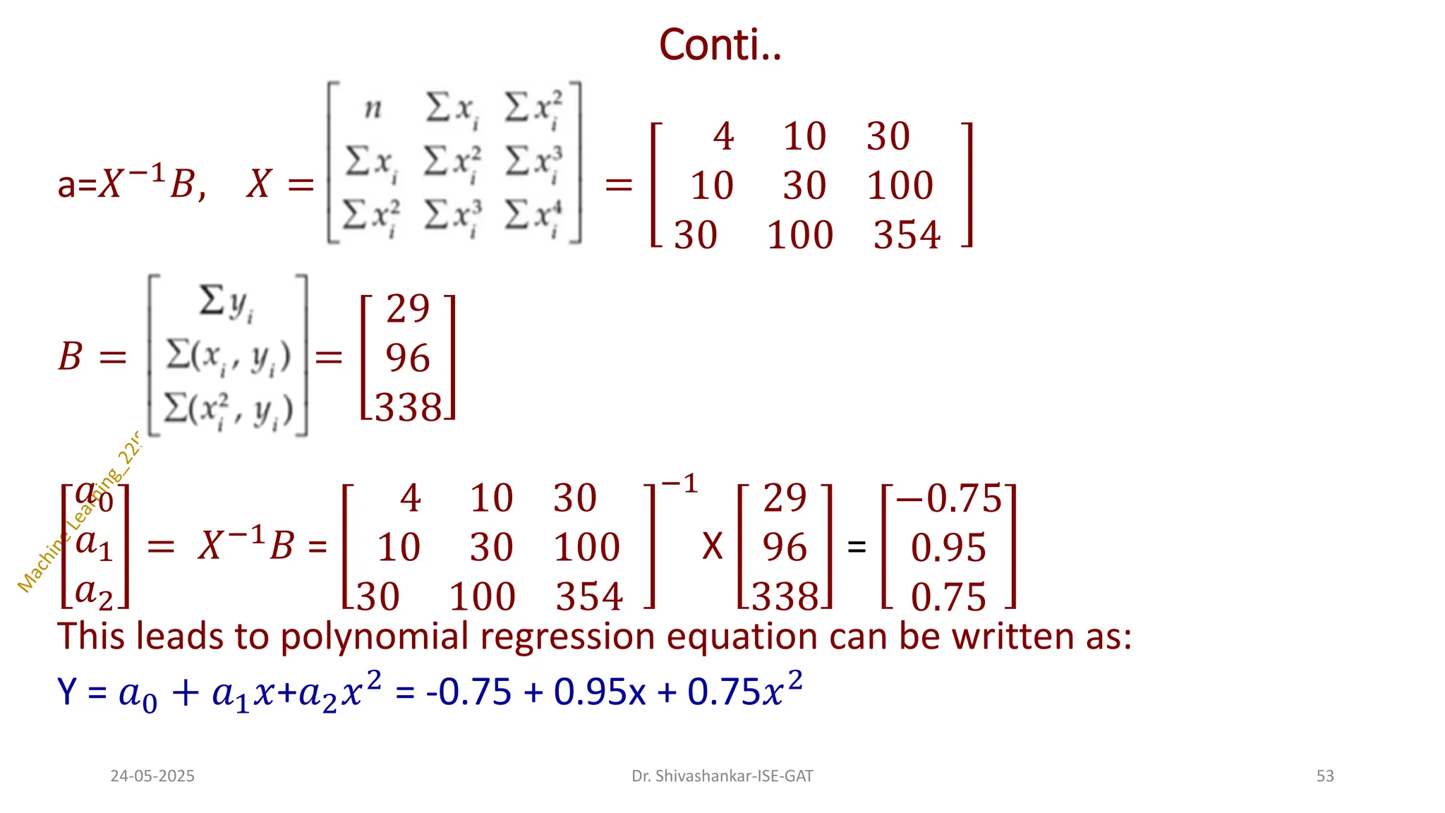
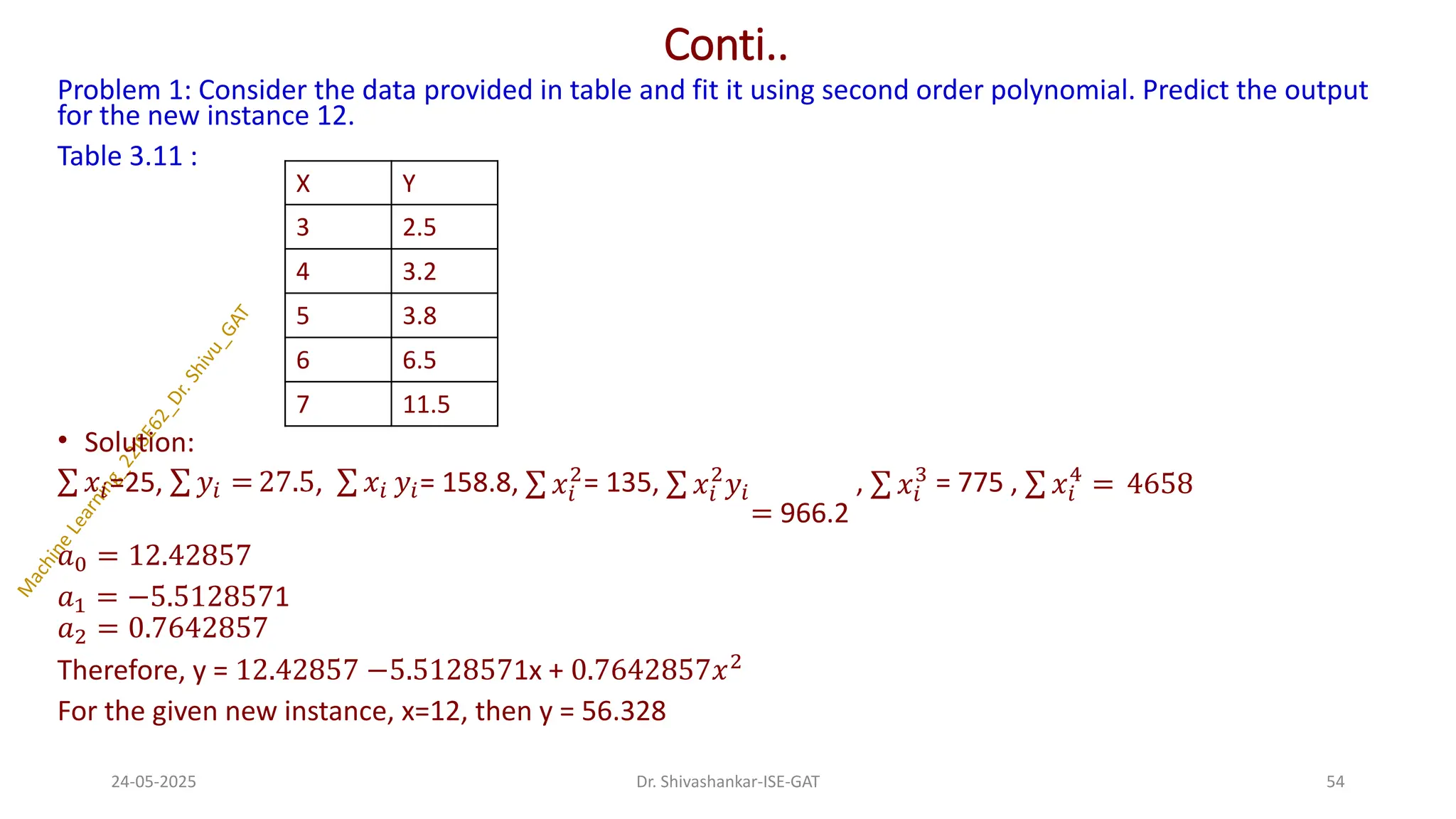
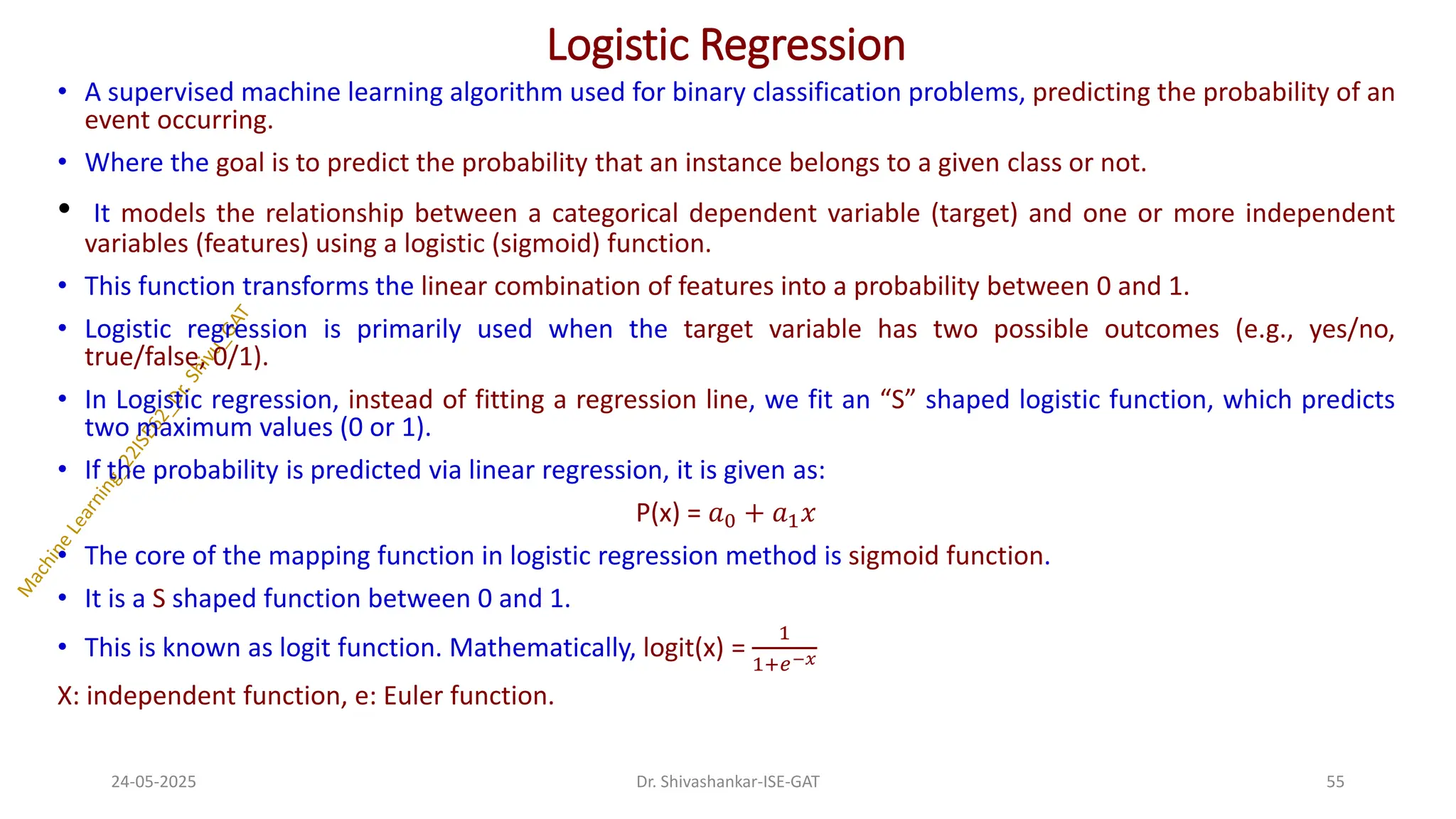
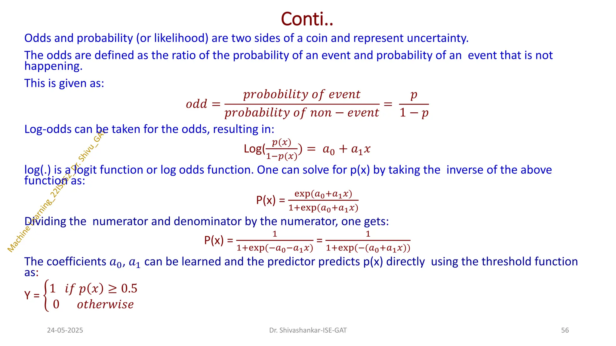
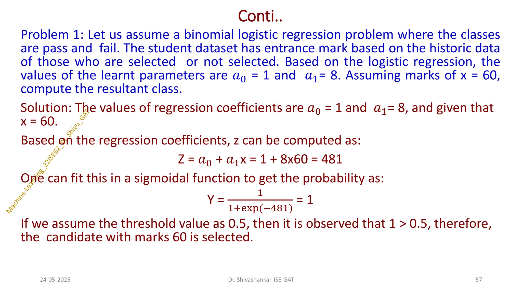
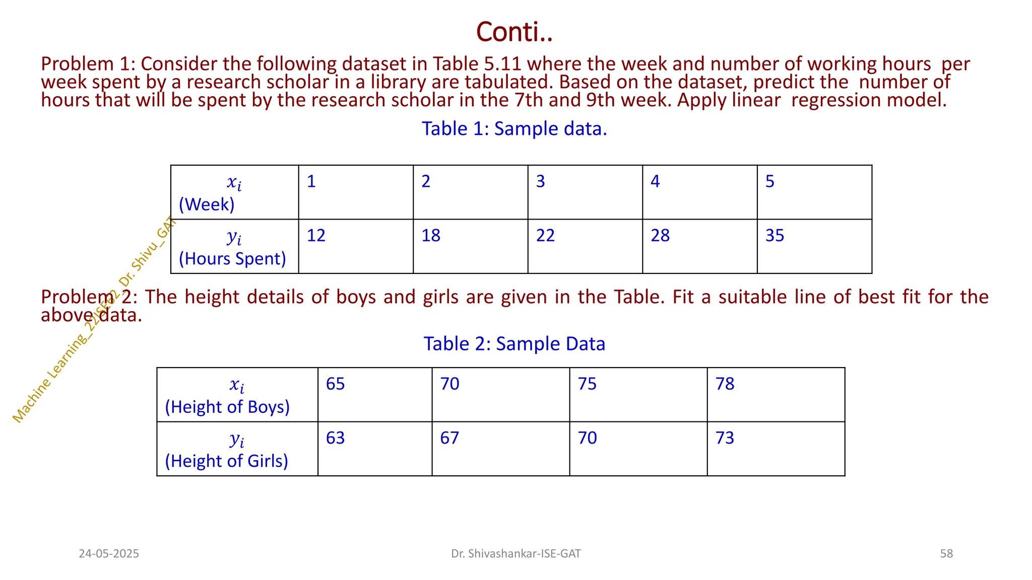
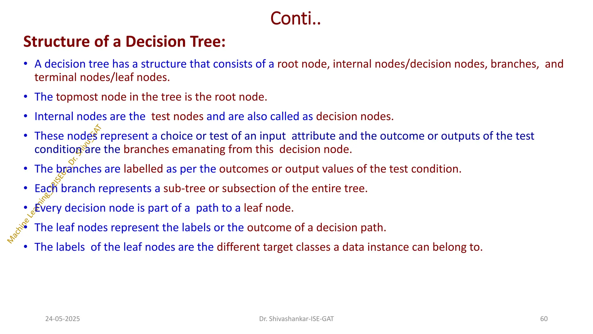
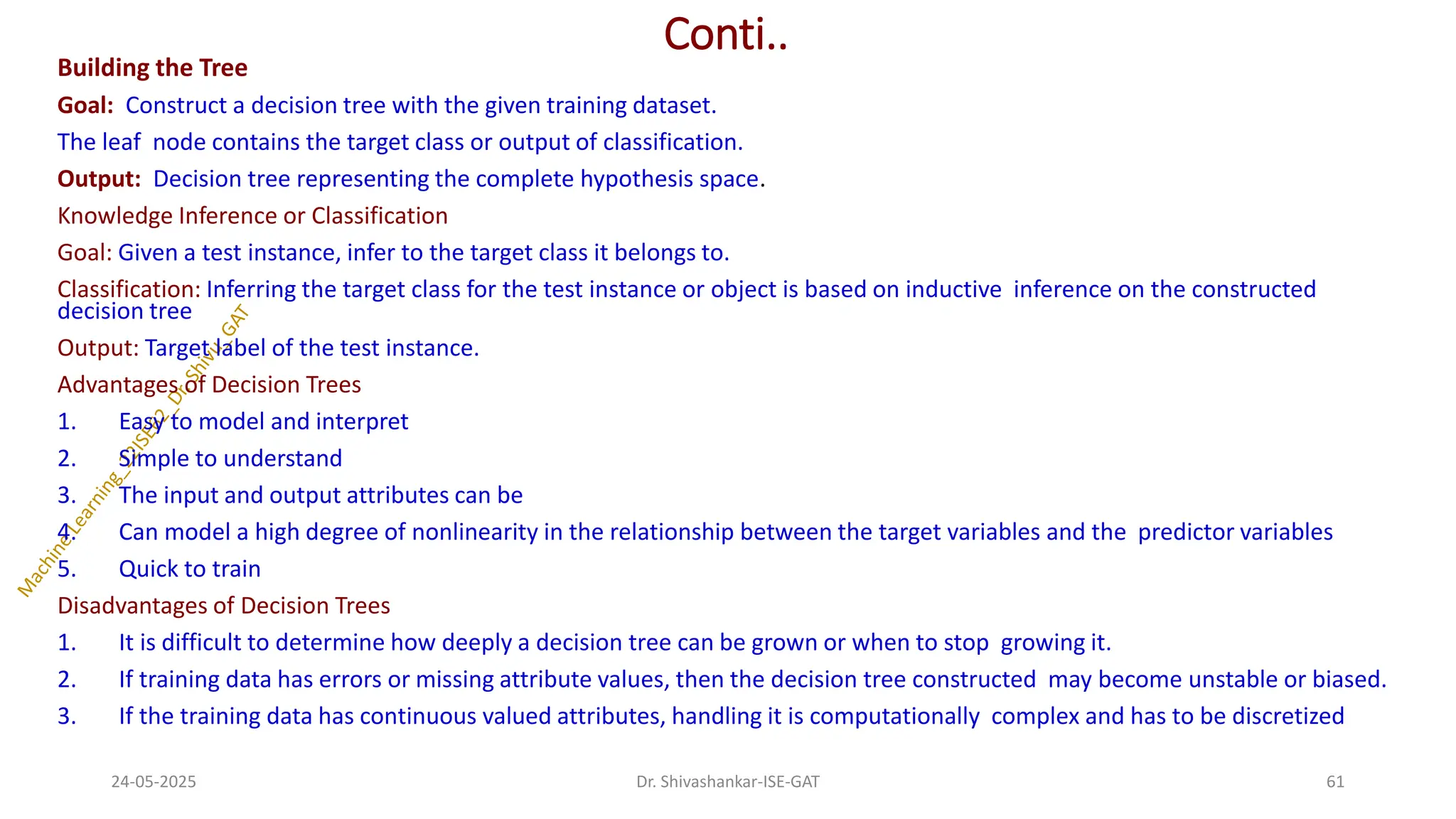
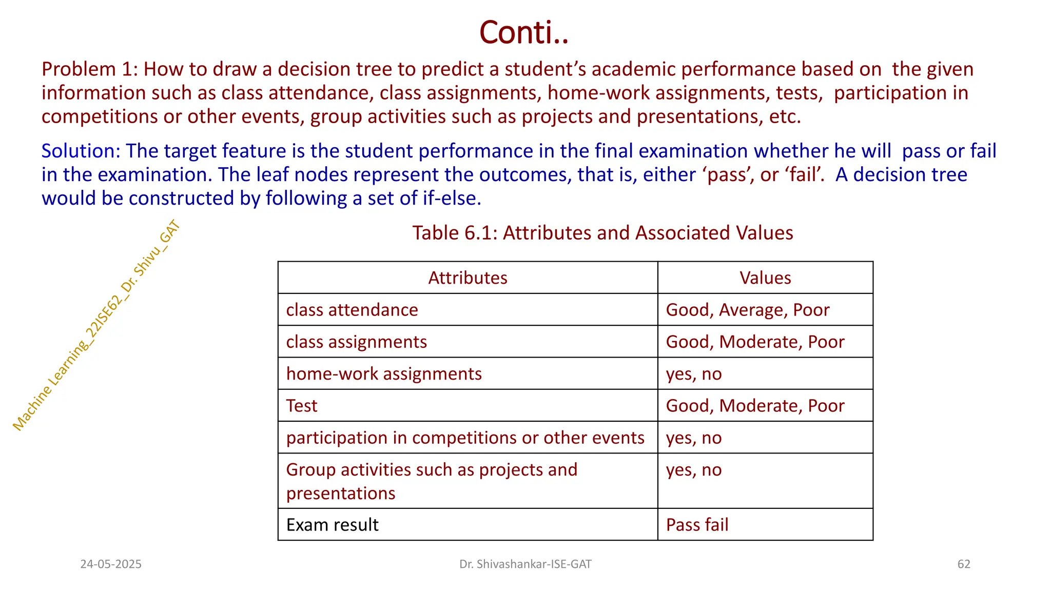
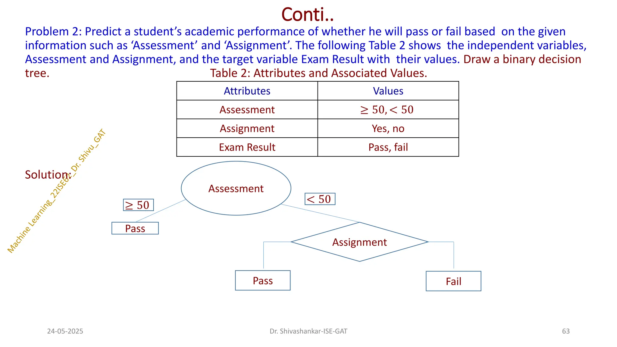
![Conti..
Let P be the probability distribution of data instances from 1 to n.
So, P = 𝑃1, 𝑃2, … … 𝑃𝑛
Entropy of P is the information measure of this probability distribution given as,
Entropy_Info(P) = Entropy_Info (𝑃1, 𝑃2, … … 𝑃𝑛) = -(𝑃1𝑙𝑜𝑔2𝑃1+𝑃2𝑙𝑜𝑔2𝑃2 +…..+𝑃𝑛𝑙𝑜𝑔2𝑃𝑛)
where, 𝑃1 is the probability of data instances classified as class 1 and 𝑃2 is the probability
of data instances classified as class 2 and so on.
𝑃1 =
|𝑁𝑜 𝑜𝑓 𝑑𝑎𝑡𝑎 𝑖𝑛𝑠𝑡𝑎𝑛𝑐𝑒𝑠 𝑏𝑒𝑙𝑜𝑛𝑔𝑖𝑛𝑔 𝑡𝑜 𝑐𝑙𝑎𝑠𝑠 1|
|𝑇𝑜𝑡𝑎𝑙 𝑛𝑜 𝑜𝑓 𝑑𝑎𝑡𝑎 𝑖𝑛𝑠𝑡𝑎𝑛𝑐𝑒𝑠 𝑖𝑛 𝑡ℎ𝑒 𝑡𝑟𝑎𝑖𝑛𝑖𝑛𝑔 𝑑𝑎𝑡𝑎𝑠𝑒𝑡|
Mathematically, entropy is defined as
Entropy_Info(X) = σ𝑥𝜖𝑣𝑎𝑙𝑢𝑒𝑠(𝑋) 𝑝𝑟 𝑋 = 𝑥 . 𝑙𝑜𝑔2
1
𝑝𝑟 𝑋=𝑥 .
Pr[X = x] is the probability of a random variable X with a possible outcome x.
24-05-2025 66
Dr. Shivashankar-ISE-GAT](https://image.slidesharecdn.com/machinelearning-module3-250524092052-1361b02d/75/Dr-Shivu__Machine-Learning-Module-3-pdf-66-2048.jpg)
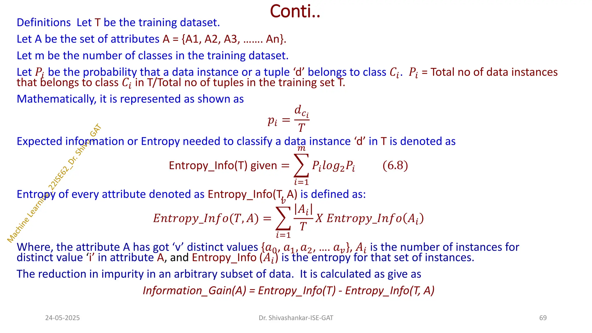
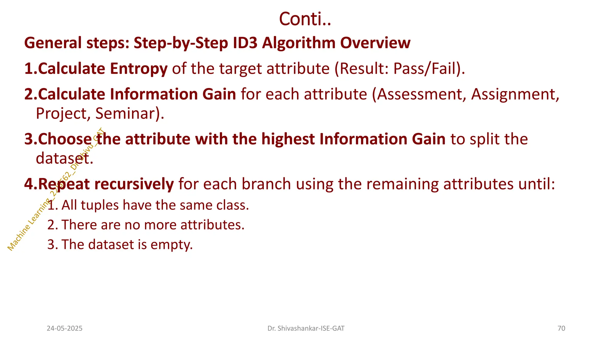
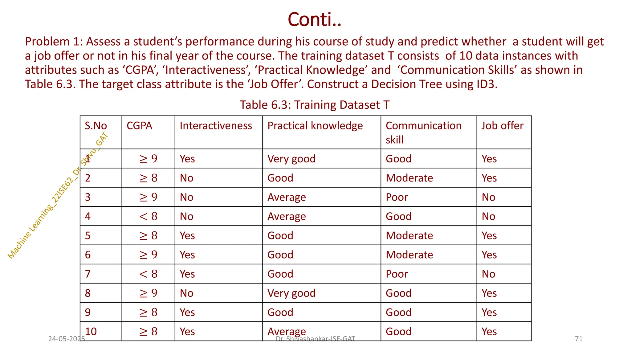
![Conti..
Solution:
Step 1: Calculate the Entropy for the target class ‛Job Offer’.
Entropy_Info(Target Attribute = Job Offer) = Entropy_Info(7, 3) = -[
7
10
𝑙𝑜𝑔2
7
10
+
3
10
𝑙𝑜𝑔2
3
10
] = -(-0.3602 + -0.5210) =
0.8812
Iteration 1:
Step 2: Calculate the Entropy_Info and Gain(Information_Gain) for each of the attribute in the training dataset.
Table 6.4 shows the number of data instances classified with Job Offer as Yes or No for the attribute CGPA.
Table 6.4: Entropy Information for CGPA CGPA
Entropy_Info(T, CGPA) =
4
10
[−
3
4
𝑙𝑜𝑔2
3
4
−
1
4
𝑙𝑜𝑔2
1
4
] +
4
10
[−
4
4
𝑙𝑜𝑔2
4
4
−
0
4
𝑙𝑜𝑔2
0
4
] +
2
10
[−
0
2
𝑙𝑜𝑔2
0
2
−
2
2
𝑙𝑜𝑔2
2
2
] = 0.3243
Gain (CGPA) = Entropy_Info(Target Attribute = Job Offer) - Entropy_Info(T, CGPA) = 0.8812 - 0.3245 = 0.5567
24-05-2025 72
Dr. Shivashankar-ISE-GAT
CGPA Job offer = Yes Job offer = No Total Entropy
≥ 9 3 1 4
≥ 8 4 0 4 0
<8 0 2 2 0](https://image.slidesharecdn.com/machinelearning-module3-250524092052-1361b02d/75/Dr-Shivu__Machine-Learning-Module-3-pdf-72-2048.jpg)
![Conti..
Table 6.5 shows the number of data instances classified with Job Offer as Yes or No for the attribute
Interactiveness.
Table 6.5: Entropy Information for Interactiveness.
Entropy_Info(T, Interactiveness) =
6
10
[−
5
6
𝑙𝑜𝑔2
5
6
−
1
6
𝑙𝑜𝑔2
1
6
] +
4
10
[−
2
4
𝑙𝑜𝑔2
2
4
− −
2
4
𝑙𝑜𝑔2
2
4
] = 0.7896
Gain(Interactiveness) = Entropy_Info(Target Attribute = Job Offer) - Entropy_Info(T, Interactiveness) = 0.8807
- 0.7896 = 0.0911
Table 6.6 shows the number of data instances classified with Job Offer as Yes or No for the attribute
Practical Knowledge. Table 6.6: Entropy Information for Practical Knowledge
24-05-2025 73
Dr. Shivashankar-ISE-GAT
Interactiveness Job offer = Yes Job offer = No Total Entropy
Yes 5 1 6
No 2 2 4
Practical
knowledge
Job offer = Yes Job offer = No Total Entropy
Very good 2 0 2 0
Good 1 2 3
Average 4 1 5](https://image.slidesharecdn.com/machinelearning-module3-250524092052-1361b02d/75/Dr-Shivu__Machine-Learning-Module-3-pdf-73-2048.jpg)
![Conti..
Entropy_Info(T, Practical Knowledge) =
2
10
[−
2
2
𝑙𝑜𝑔2
2
2
−
0
2
𝑙𝑜𝑔2
0
2
] +
3
10
[−
1
3
𝑙𝑜𝑔2
1
3
−
2
3
𝑙𝑜𝑔2
2
3
] +
5
10
[−
4
5
𝑙𝑜𝑔2
4
5
−
−
1
5
𝑙𝑜𝑔2
1
5
] = 0.6361
Gain(Practical Knowledge) = Entropy_Info(Target Attribute = Job Offer) - Entropy_Info(T, Practical Knowledge) =
0.8807 - 0.6361 = 0.2446
Table 6.7 shows the number of data instances classified with Job Offer as Yes or No for the attribute
Communication Skills. Table 6.7: Entropy Information for Communication Skills
Entropy_Info(T, Communication Skills) =
5
10
[−
4
5
𝑙𝑜𝑔2
4
5
−
1
5
𝑙𝑜𝑔2
1
5
] +
3
10
[−
3
3
𝑙𝑜𝑔2
3
3
− −
0
3
𝑙𝑜𝑔2
0
3
] +
2
10
[−
0
2
𝑙𝑜𝑔2
0
2
−
2
2
𝑙𝑜𝑔2
2
2
] = 0.3609
Gain(Communication Skills) = Entropy_Info(Target Attribute = Job Offer) - Entropy_Info(T, Communication Skills) =
0.8813 - 0.36096 = 0.5203
24-05-2025 74
Dr. Shivashankar-ISE-GAT
Communication Skill Job offer = Yes Job offer = No Total
Good 4 1 5
Moderate 3 0 3
Poor 0 2 2](https://image.slidesharecdn.com/machinelearning-module3-250524092052-1361b02d/75/Dr-Shivu__Machine-Learning-Module-3-pdf-74-2048.jpg)
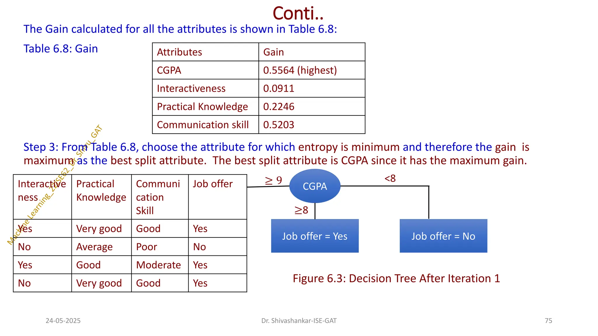
![Conti..
Now, continue the same process for the subset of data instances branched with CGPA ≥ 9 (Highest attributes)
Iteration 2: In this iteration, the same process of computing the Entropy_Info and Gain are repeated with the
subset of training set. Job Offer has 3 instances as Yes and 1 instance as No.
Entropy_Info(T) = Entropy_Info(3, 1) = - [
3
4
𝑙𝑜𝑔2
3
4
+
1
4
𝑙𝑜𝑔2
1
4
] = 0.8112
Entropy_Info(T, Interactiveness) =
2
4
[−
2
2
𝑙𝑜𝑔2
2
2
−
0
2
𝑙𝑜𝑔2
0
2
] +
2
4
[−
1
2
𝑙𝑜𝑔2
1
2
−
1
2
𝑙𝑜𝑔2
1
2
] = 0.4997
Gain(Interactiveness) = 0.8112 - 0.4997 = 0.3115
Entropy_Info(T, Practical Knowledge) =
2
4
[−
2
2
𝑙𝑜𝑔2
2
2
−
0
2
𝑙𝑜𝑔2
0
2
] +
1
4
[−
1
1
𝑙𝑜𝑔2
1
1
−
1
1
𝑙𝑜𝑔2
1
1
] +
1
4
[−
1
1
𝑙𝑜𝑔2
1
1
−
1
1
𝑙𝑜𝑔2
1
1
] = 0
Gain(Practical Knowledge) = 0.8112
Entropy_Info(T, Communication Skills) =
2
4
[−
2
2
𝑙𝑜𝑔2
2
2
−
0
2
𝑙𝑜𝑔2
0
2
] +
1
4
[−
1
1
𝑙𝑜𝑔2
1
1
−
1
1
𝑙𝑜𝑔2
1
1
] +
1
4
[−
1
1
𝑙𝑜𝑔2
1
1
−
1
1
𝑙𝑜𝑔2
1
1
] = 0
Gain (Communication Skills) = 0.8112
The gain calculated for all the attributes is shown in Table 6.9.
24-05-2025 76
Dr. Shivashankar-ISE-GAT
Attributes Gain
Interactiveness 0.3111
Practical knowledge 0.8112
Communication skill 0.8112
Interactiveness Job offer=Yes Job Offer = No
Yes 2 0
No 1 1](https://image.slidesharecdn.com/machinelearning-module3-250524092052-1361b02d/75/Dr-Shivu__Machine-Learning-Module-3-pdf-76-2048.jpg)
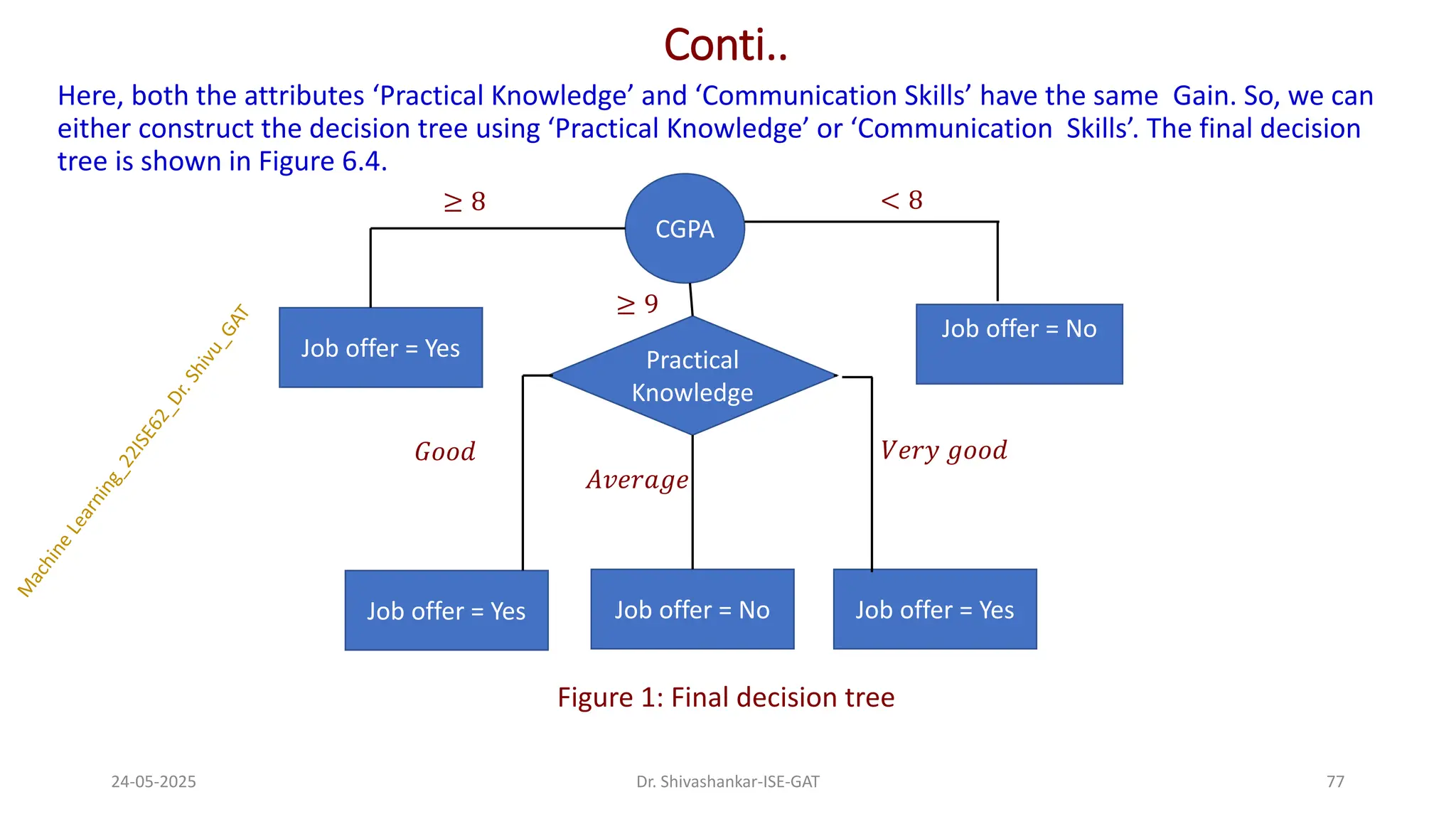
![Problems
Problem 1: Construct decision tree using ID3, considering the following example.
Solution:
Attribute : a1
Values(a1)=True / False
S=[6+,4-], Entropy (S)= -
6
10
log2
6
10
−
4
10
log2
4
10
= 0.9709
𝑆𝑇𝑟𝑢𝑒=[1+,4-], Entropy (𝑆𝑇𝑟𝑢𝑒)= -
1
5
log2
1
5
−
4
5
log2
4
5
= 0.7219
𝑆𝐹𝑎𝑙𝑠𝑒=[5+,0-], Entropy (𝑆𝐹𝑎𝑙𝑠𝑒)= -
5
5
log2
5
5
−
0
5
log2
0
5
= 0.0
Gain (S,a1)= Entropy (S) - σ𝑣𝜖{𝑇𝑟𝑢𝑒𝑠,𝑓𝑎𝑙𝑠𝑒}
𝑆𝑣
𝑆
𝐸𝑛𝑡𝑟𝑜𝑝𝑦(𝑆𝑣)
Gain (S,a1)=Entropy (S) -
5
10
Entropy (𝑆𝑇𝑟𝑢𝑒) -
5
10
Entropy (𝑆𝐹𝑎𝑙𝑠𝑒)
= 0.9709 -
5
10
X0.7219 -
5
10
X0.0= 0.6099
5/24/2025 78
Dr. Shivashankar, ISE, GAT
Instance a1 a2 a3 Classifi
cation
1 True Hot High No
2 True Hot High No
3 False Hot High Yes
4 False Cool Normal Yes
5 False Cool Normal Yes
6 True Cool High No
7 True Hot High No
8 True Hot Normal Yes
9 False Cool Normal Yes
10 False Cool High Yes
Yes No
Yes No](https://image.slidesharecdn.com/machinelearning-module3-250524092052-1361b02d/75/Dr-Shivu__Machine-Learning-Module-3-pdf-78-2048.jpg)
![Cont…
Attribute : a2
Values(a2)=Hot, Cool
S=[6+,4-], Entropy (S)= -
6
10
log2
6
10
−
4
10
log2
4
10
= 0.9709
𝑆𝐻𝑜𝑡=[2+, 3-], Entropy (𝑆𝐻𝑜𝑡)= -
2
5
log2
2
5
−
3
5
log2
3
5
= 0.9709
𝑆𝐶𝑜𝑜𝑙=[4+,1-], Entropy (𝑆𝐶𝑜𝑜𝑙)= -
4
5
log2
4
5
−
1
5
log2
1
5
= 0.7219
Gain (S,a2)= Entropy (S) - σ𝑣𝜖{𝐻𝑜𝑡,𝐶𝑜𝑜𝑙}
𝑆𝑣
𝑆
𝐸𝑛𝑡𝑟𝑜𝑝𝑦(𝑆𝑣)
Gain (S,a2)=Entropy (S) -
5
10
Entropy (𝑆𝐻𝑜𝑡) -
5
10
Entropy (𝑆𝐶𝑜𝑜𝑙)
= 0.9709 -
5
10
X0.9709 -
5
10
X0.7219= 0.1245
Attribute : a3
Values(a3)=High, Normal
S=[6+,4-] Entropy (S)= -
6
10
log2
6
10
−
4
10
log2
4
10
= 0.9709
𝑆𝐻𝑖𝑔ℎ=[2+, 4-] Entropy (𝑆𝐻𝑖𝑔ℎ)= -
2
6
log2
2
6
−
4
5
log2
4
5
= 0.9183
𝑆𝑁𝑜𝑟𝑚𝑎𝑙=[4+,0-] Entropy (𝑆𝑁𝑜𝑟𝑚𝑎𝑙)= -
4
4
log2
4
4
−
0
4
log2
0
4
= 0.0
Gain (S,a3)= Entropy (S) - σ𝑣𝜖{𝐻𝑖𝑔ℎ,𝑁𝑜𝑟𝑚𝑎𝑙}
𝑆𝑣
𝑆
𝐸𝑛𝑡𝑟𝑜𝑝𝑦(𝑆𝑣)
Gain (S,a3)=Entropy (S) -
6
10
Entropy (𝑆𝐻𝑖𝑔ℎ) −
4
10
Entropy (𝑆𝑁𝑜𝑟𝑚𝑎𝑙) = 0.9709 -
6
10
X0.9183 -
4
10
X0.0
5/24/2025 79
Dr. Shivashankar, ISE, GAT](https://image.slidesharecdn.com/machinelearning-module3-250524092052-1361b02d/75/Dr-Shivu__Machine-Learning-Module-3-pdf-79-2048.jpg)
![Cont…
∴ Gain (S,a1)= 0.6099- Maximum
Gain (S,a2)= 0.1245
Gain (S,a3)= 0.4199
Attribute : a2
Values(a2)=Hot, Cool
𝑆𝑎2=[1+,4-] Entropy (𝑆𝑎2)= -
1
5
log2
1
5
−
4
5
log2
4
5
= 0.7219
𝑆𝐻𝑜𝑡=[1+, 3-] Entropy (𝑆𝐻𝑜𝑡)= -
1
4
log2
1
4
−
3
4
log2
3
4
= 0.8112
𝑆𝐶𝑜𝑜𝑙=[0+,1-] Entropy (𝑆𝐶𝑜𝑜𝑙)= -
0
1
log2
0
1
−
1
1
log2
1
1
= 0.0
Gain (S,a2)= Entropy (S) - σ𝑣𝜖{𝐻𝑜𝑡,𝐶𝑜𝑜𝑙}
𝑆𝑣
𝑆
𝐸𝑛𝑡𝑟𝑜𝑝𝑦(𝑆𝑣)
Gain (S,a2)=Entropy (S) -
4
5
Entropy (𝑆𝐻𝑜𝑡) -
1
5
Entropy (𝑆𝐶𝑜𝑜𝑙)
5/24/2025 80
Dr. Shivashankar, ISE, GAT
a1
True False
1,2,6,7,8 3,4,5,9,10
Yes
Instance a2 a3 Classific
ation
1 Hot High No
2 Hot High No
6 Cool High No
7 Hot High No
8 Hot Normal Yes
?](https://image.slidesharecdn.com/machinelearning-module3-250524092052-1361b02d/75/Dr-Shivu__Machine-Learning-Module-3-pdf-80-2048.jpg)
![Cont…
Attribute : a3
Values(a3)=High, Normal
𝑆𝑎3=[1+,4-] Entropy (𝑆𝑎3)= -
1
5
log2
1
5
−
4
5
log2
4
5
= 0.7219
𝑆𝐻𝑖𝑔ℎ=[0+, 4-] Entropy (𝑆𝐻𝑖𝑔ℎ)= -
0
4
log2
0
4
−
4
4
log2
4
4
= 0.0
𝑆𝑁𝑜𝑟𝑚𝑎𝑙=[1+,0-] Entropy (𝑆𝑁𝑜𝑟𝑚𝑎𝑙)= -
1
1
log2
1
1
−
0
1
log2
0
1
= 0.0
Gain (S,a3)= Entropy (S) - σ𝑣𝜖{𝐻𝑖𝑔ℎ,𝑁𝑜𝑟𝑚𝑎𝑙}
𝑆𝑣
𝑆
𝐸𝑛𝑡𝑟𝑜𝑝𝑦(𝑆𝑣)
Gain (S,a3)=Entropy (S) -
4
5
Entropy (𝑆𝐻𝑖𝑔ℎ) -
1
5
Entropy (𝑆𝑁𝑜𝑟𝑚𝑎𝑙) = 0.9709 -
4
5
X0.0 -
1
5
X0.0
= 0.9709
∴ Gain (Sa1,a2)=0.3210
Gain(Sa1, a3)=0.9709---Maximum
5/24/2025 81
Dr. Shivashankar, ISE, GAT
a1
True False
1,2,6,7,8 3,4,5,9,10
a3
1,2,6,7 8
High Normal
Yes
Yes
No](https://image.slidesharecdn.com/machinelearning-module3-250524092052-1361b02d/75/Dr-Shivu__Machine-Learning-Module-3-pdf-81-2048.jpg)

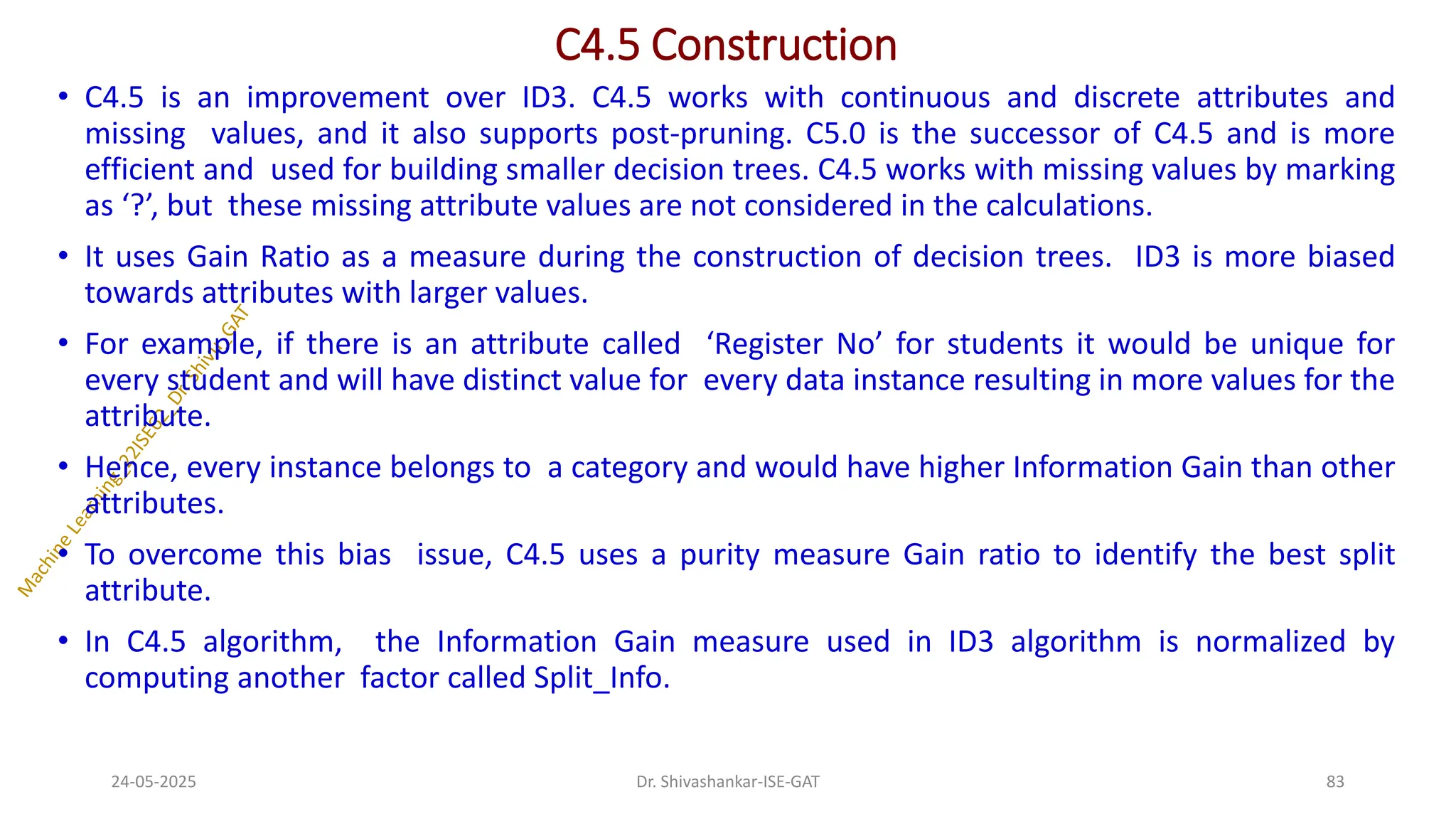
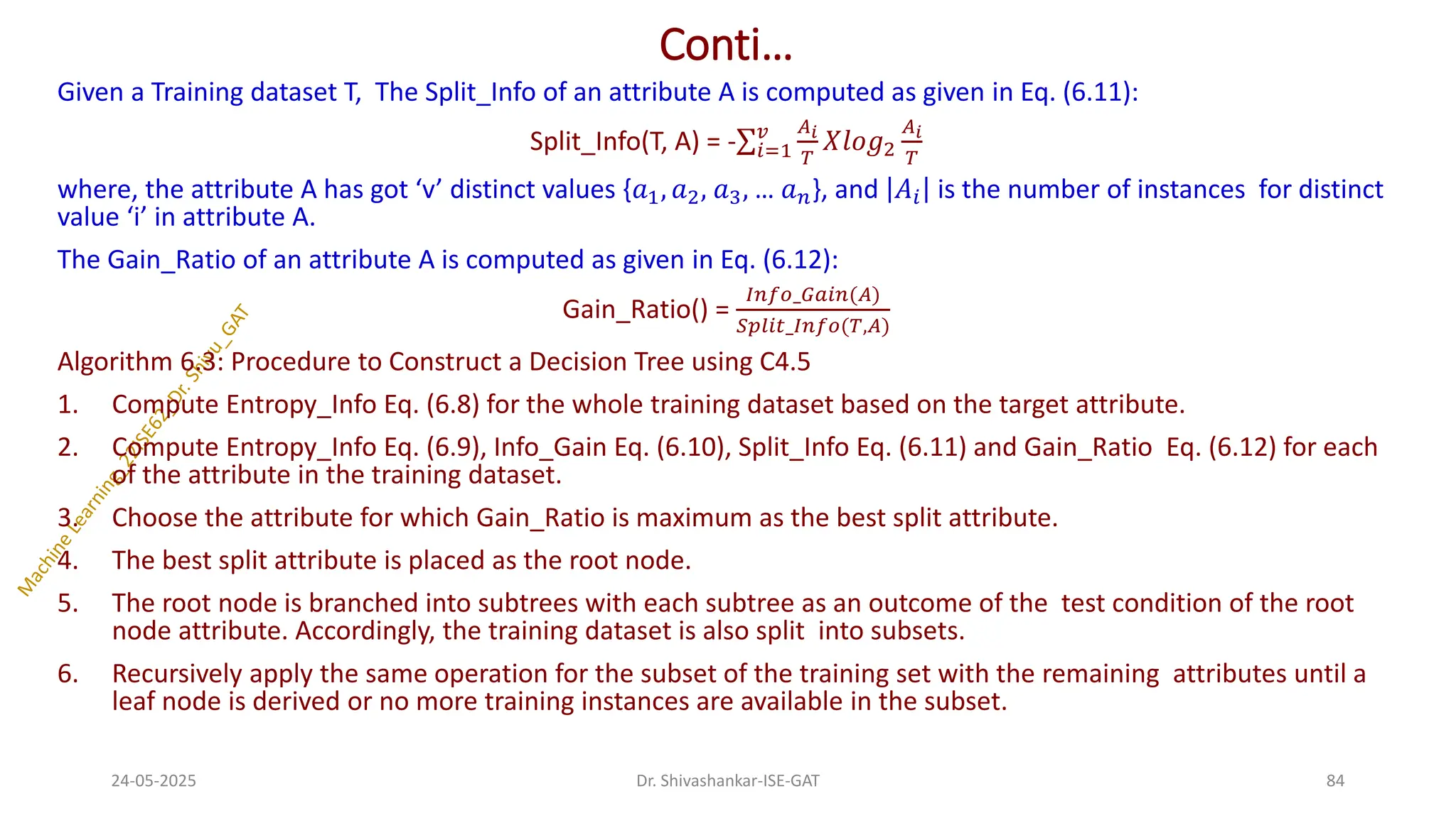
![Conti..
Example 6.4: Make use of Information Gain of the attributes which are calculated in ID3 algorithm in
Example 6.3 to construct a decision tree using C4.5.
Solution: Iteration 1:
Step 1: Calculate the Class_Entropy for the target class ‘Job Offer’. Entropy_Info(Target Attribute = Job Offer)
= Entropy_Info(7, 3) = −[
7
10
𝑙𝑜𝑔2
7
10
+
3
10
𝑙𝑜𝑔2
3
10
] = 0.8807
Step 2: Calculate the Entropy_Info, Gain(Info_Gain), Split_Info, Gain_Ratio for each of the attribute in the
training dataset.
CGPA:
Entropy Info(T, CGPA) =
4
10
[−
3
4
𝑙𝑜𝑔2
3
4
−
1
4
𝑙𝑜𝑔2
1
4
] +
4
10
[−
4
4
𝑙𝑜𝑔2
4
4
−
0
4
𝑙𝑜𝑔2
0
4
] +
2
10
[−
0
2
𝑙𝑜𝑔2
0
2
−
2
2
𝑙𝑜𝑔2
2
2
] =
0.3243
Gain(CGPA) = 0.8807 - 0.3243 = 0.5564
Split _ Info(, CGPA) = −
4
10
𝑙𝑜𝑔2
4
10
−
4
10
𝑙𝑜𝑔2
4
10
−
2
10
𝑙𝑜𝑔2
2
10
= 1.5211
Gain Ratio(CGPA) =
(Gain(CGPA))
Split_Info(T, CGPA))
=
0.5564
1.5211
= 0.3658
24-05-2025 85
Dr. Shivashankar-ISE-GAT
CGPA ≥ 9 = 4, ≥ 8 = 4, < 8 = 2](https://image.slidesharecdn.com/machinelearning-module3-250524092052-1361b02d/75/Dr-Shivu__Machine-Learning-Module-3-pdf-85-2048.jpg)
![Conti..
Interactiveness: Entropy Info(T, Interactiveness) =
6
10
[−
5
6
𝑙𝑜𝑔2
5
6
−
1
6
𝑙𝑜𝑔2
1
6
] +
4
10
[−
2
4
𝑙𝑜𝑔2
2
4
−
2
4
𝑙𝑜𝑔2
2
4
] =
0.7896
Gain(Interactiveness) = 0.8807 - 0.7896 = 0.0911
Split _ Info(T, Interactiveness) = −
6
10
𝑙𝑜𝑔2
6
10
−
4
10
𝑙𝑜𝑔2
4
10
= 0.9704
Gain_Ratio(Interactiveness) =
Gain(Interactiveness)
Split _ Info(, Interactiveness)
=
0.0911
0.9704
= 0.0939
Practical Knowledge:
Entropy_Info(T, Practical Knowledge) =
2
10
[−
2
2
𝑙𝑜𝑔2
2
2
−
0
2
𝑙𝑜𝑔2
0
2
] +
3
10
[−
1
3
𝑙𝑜𝑔2
1
3
−
2
3
𝑙𝑜𝑔2
2
3
] +
5
10
[−
4
5
𝑙𝑜𝑔2
4
5
−
1
5
𝑙𝑜𝑔2
1
5
] = 0.6361
Gain(Practical Knowledge) = 0.8807 - 0.6361 = 0.2448
Split_Info(T, Practical Knowledge) = −
2
10
𝑙𝑜𝑔2
2
10
−
5
10
𝑙𝑜𝑔2
5
10
−
3
10
𝑙𝑜𝑔2
3
10
= 1.4853
Gain_Ratio(Practical Knowledge) = −
Gain(Practical Knowledge)
Split _ Info(, Practical Knowledge)
=
0.2448
1.4853
= 0.1648
24-05-2025 86
Dr. Shivashankar-ISE-GAT](https://image.slidesharecdn.com/machinelearning-module3-250524092052-1361b02d/75/Dr-Shivu__Machine-Learning-Module-3-pdf-86-2048.jpg)
![Conti..
Communication Skills:
Entropy_Info(T, Communication Skills) =
5
10
[−
4
5
𝑙𝑜𝑔2
4
5
−
1
5
𝑙𝑜𝑔2
1
5
] +
3
10
[−
3
3
𝑙𝑜𝑔2
3
3
−
0
3
𝑙𝑜𝑔2
0
3
] +
2
10
[−
0
2
𝑙𝑜𝑔2
0
2
−
2
2
𝑙𝑜𝑔2
2
2
] = 0.3609
Gain(Communication Skills) = 0.8813 - 0.36096 = 0.5202
Split _ Info(T, Communication Skills) = −
5
10
𝑙𝑜𝑔2
5
10
−
3
10
𝑙𝑜𝑔2
3
10
−
2
10
𝑙𝑜𝑔2
2
10
= 1.4853
Gain_Ratio(Communication Skills) =
Gain(Communication Skills)
Split_Info(T, Communication Skills)
=
0.5202
1.4853
= 0.3502
Table 6.10: Gain_Ratio
24-05-2025 87
Dr. Shivashankar-ISE-GAT
Attributes Gain Ratio
CGPA 0.3658
Interactiveness 0.0939
Practical Knowledge 0.1648
Communication skill 0.3502](https://image.slidesharecdn.com/machinelearning-module3-250524092052-1361b02d/75/Dr-Shivu__Machine-Learning-Module-3-pdf-87-2048.jpg)
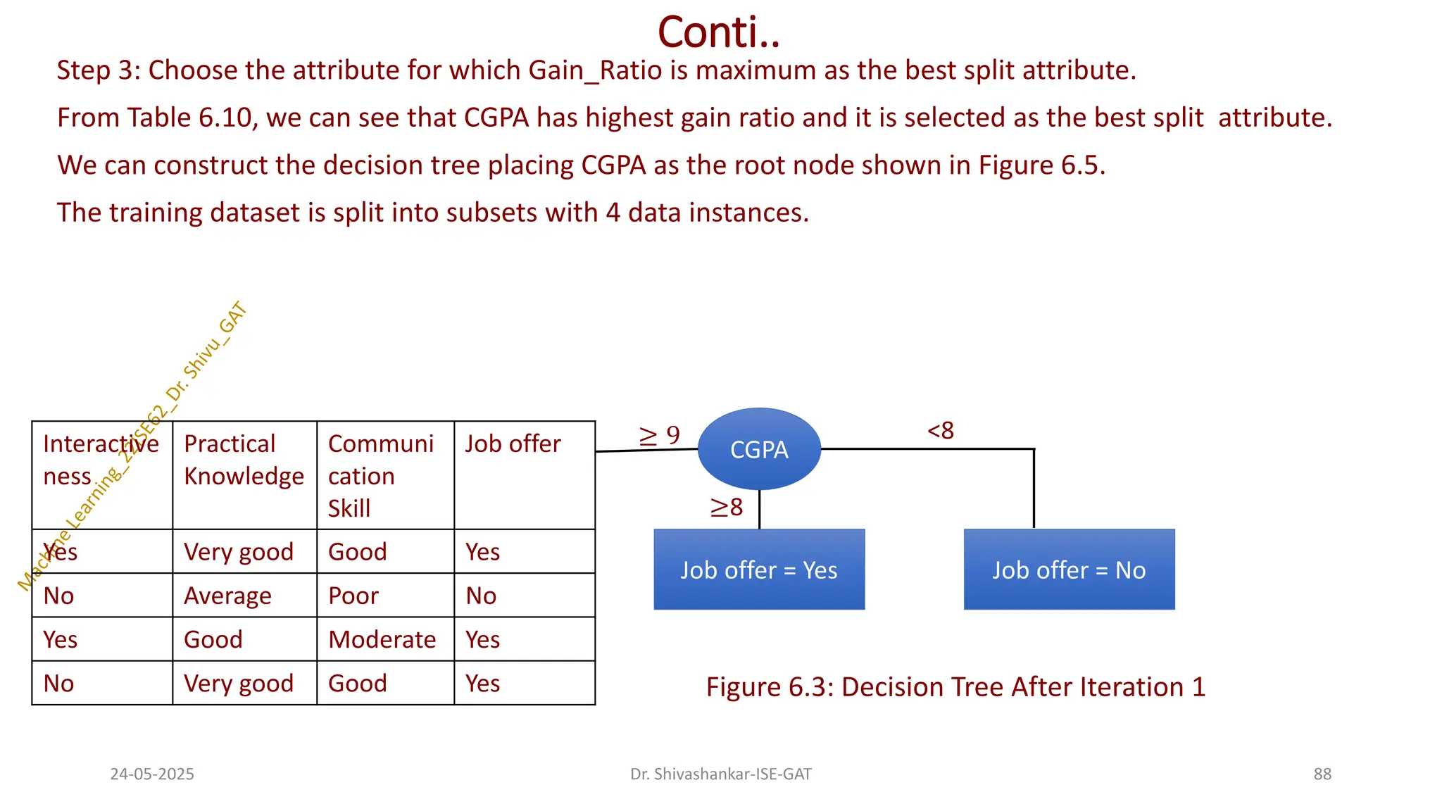
![Conti..
Iteration 2:
Total Samples: 4 Repeat the same process for this resultant dataset with 4 data instances.
Job Offer has 3 instances as Yes and 1 instance as No.
Entropy_Info(Target Class = Job Offer) = −
3
4
𝑙𝑜𝑔2
3
4
−
1
4
𝑙𝑜𝑔2
1
4
= 0.8112
Interactiveness: Entropy_Info(T, Interactiveness) =
2
4
[−
2
2
𝑙𝑜𝑔2
2
2
−
0
2
𝑙𝑜𝑔2
0
2
] +
2
4
[−
1
2
𝑙𝑜𝑔2
1
2
−
1
2
𝑙𝑜𝑔2
1
2
] = 0.4997
Gain(Interactiveness) = 0.8108 - 0.4997 = 0.3111
Split _ Info(T, Interactiveness) = −
2
4
𝑙𝑜𝑔2
2
4
−
2
4
𝑙𝑜𝑔2
2
4
= 1
Gain_Ratio(Interactiveness) =
𝐺𝑎𝑖𝑛 ( 𝐼𝑛𝑡𝑒𝑟𝑎𝑐𝑡𝑖𝑣𝑒𝑛𝑒𝑠𝑠)
Split _ Info(T, Interactiveness)
=
0.3112
1
= 0.3112
Practical Knowledge:
Entropy_Info(T, Practical Knowledge) =
2
4
[−
2
2
𝑙𝑜𝑔2
2
2
−
0
2
𝑙𝑜𝑔2
0
2
] +
1
4
[−
0
1
𝑙𝑜𝑔2
0
1
−
1
1
𝑙𝑜𝑔2
1
1
] +
1
4
[−
1
1
𝑙𝑜𝑔2
1
1
−
0
1
𝑙𝑜𝑔2
0
1
]
= 0
Gain(Practical Knowledge) = 0.8108
Split_Info(T, Practical Knowledge) = −
2
4
𝑙𝑜𝑔2
2
4
−
1
4
𝑙𝑜𝑔2
1
4
−
1
4
𝑙𝑜𝑔2
1
4
= 1.5
24-05-2025 89
Dr. Shivashankar-ISE-GAT](https://image.slidesharecdn.com/machinelearning-module3-250524092052-1361b02d/75/Dr-Shivu__Machine-Learning-Module-3-pdf-89-2048.jpg)
![Conti..
Gain_Ratio(Practical Knowledge) =
𝐺𝑎𝑖𝑛 ( 𝑝𝑟𝑎𝑐𝑡𝑖𝑐𝑎𝑙 𝑘𝑛𝑜𝑤𝑙𝑒𝑑𝑔𝑒)
Split _ Info(T, 𝑝𝑟𝑎𝑐𝑡𝑖𝑐𝑎𝑙 𝑘𝑛𝑜𝑤𝑙𝑒𝑑𝑔𝑒)
=
0.8108
1.5
= 0.5408
Communication Skills: Entropy_Info(T, Communication Skills) =
2
4
[−
2
2
𝑙𝑜𝑔2
2
2
−
0
2
𝑙𝑜𝑔2
0
2
] +
1
4
[−
0
1
𝑙𝑜𝑔2
0
1
−
1
1
𝑙𝑜𝑔2
1
1
] +
1
4
[−
1
1
𝑙𝑜𝑔2
1
1
−
0
1
𝑙𝑜𝑔2
0
1
] =0
Gain(Communication Skills) = 0.8108
Split_Info(T, Practical Knowledge) = −
2
4
𝑙𝑜𝑔2
2
4
−
1
4
𝑙𝑜𝑔2
1
4
−
1
4
𝑙𝑜𝑔2
1
4
= 1.5
Gain_Ratio(Practical Knowledge) =
𝐺𝑎𝑖𝑛 ( 𝐶𝑜𝑚𝑚𝑢𝑛𝑖𝑐𝑎𝑡𝑖𝑜𝑛 𝑠𝑘𝑖𝑙𝑙)
Split _ Info(T, 𝐶𝑜𝑚𝑚𝑢𝑛𝑖𝑐𝑎𝑡𝑖𝑜𝑛 𝑠𝑘𝑖𝑙𝑙)
=
0.8108
1.5
= 0.5408
Table 6.11 shows the Gain_Ratio computed for all the attributes.
Table 6.11: Gain-Ratio Attributes
Both ‘Practical Knowledge’ and ‘Communication Skills’ have the highest gain ratio. So, the best splitting attribute
can either be ‘Practical Knowledge’ or ‘Communication Skills’, and therefore, the split can be based on any one of
these.
24-05-2025 90
Dr. Shivashankar-ISE-GAT
Attributes Gain Ration
Interactiveness 0.3112
Practical Knowledge 0.5408
Communication skill 05408](https://image.slidesharecdn.com/machinelearning-module3-250524092052-1361b02d/75/Dr-Shivu__Machine-Learning-Module-3-pdf-90-2048.jpg)

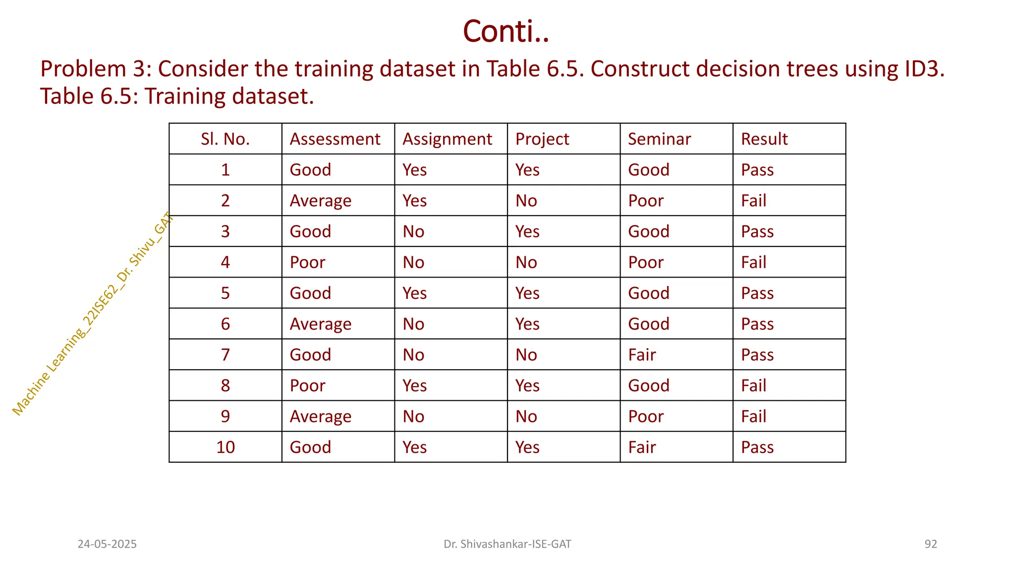
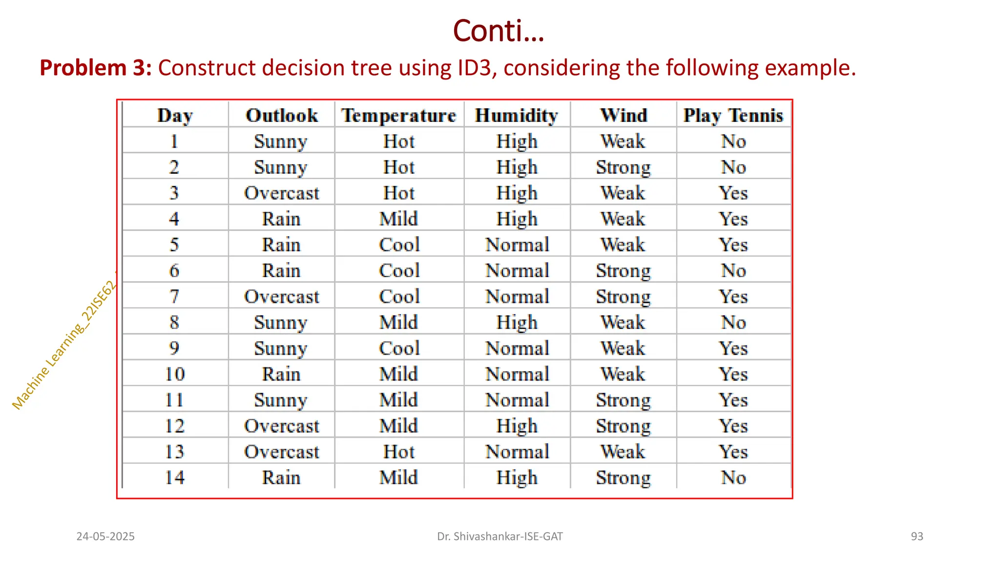
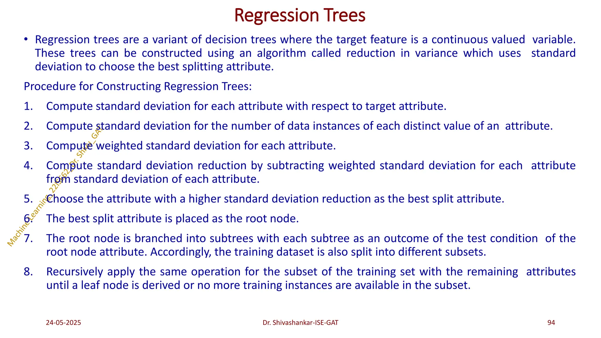
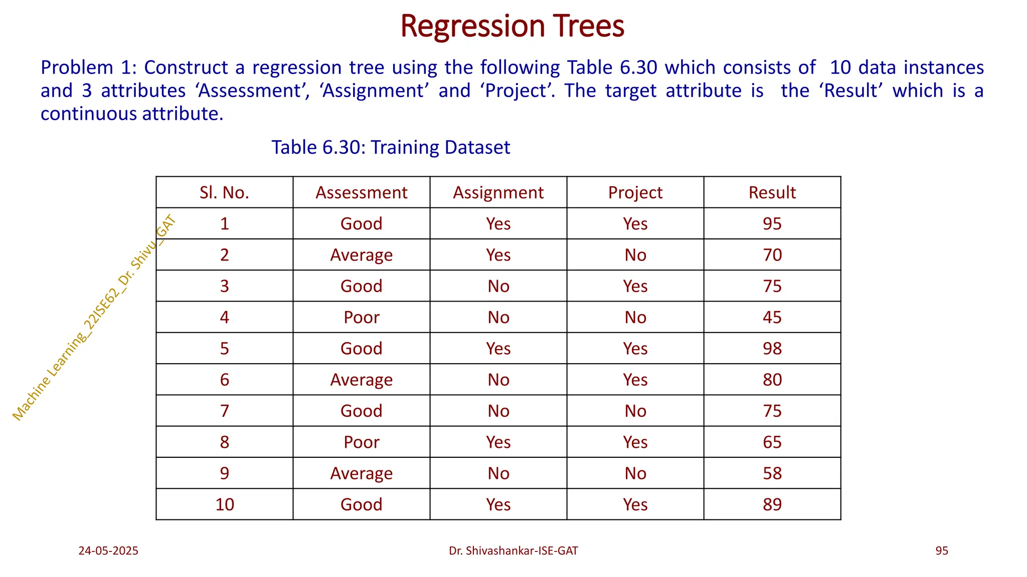
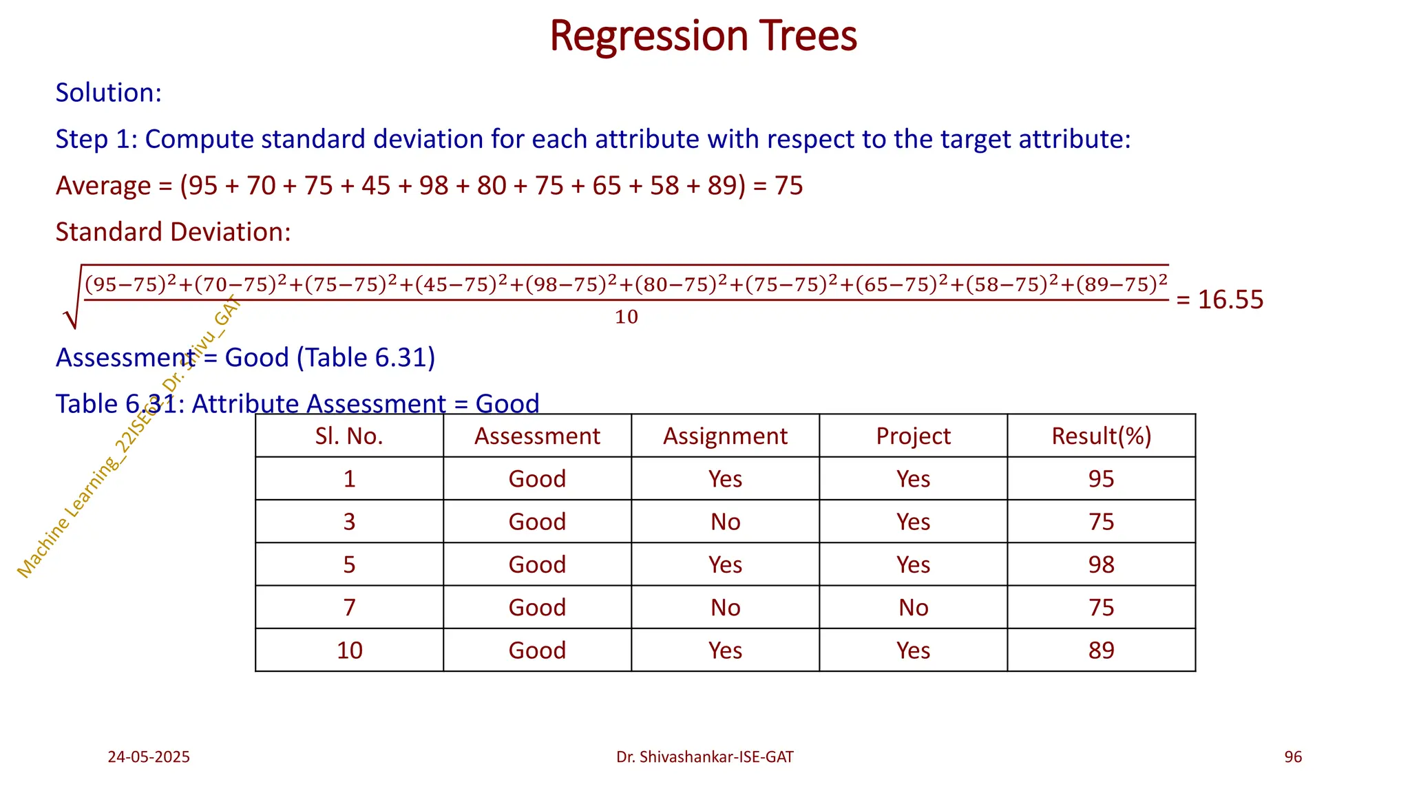
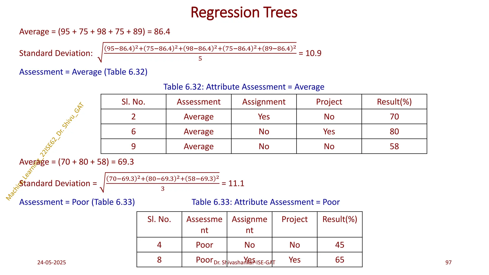
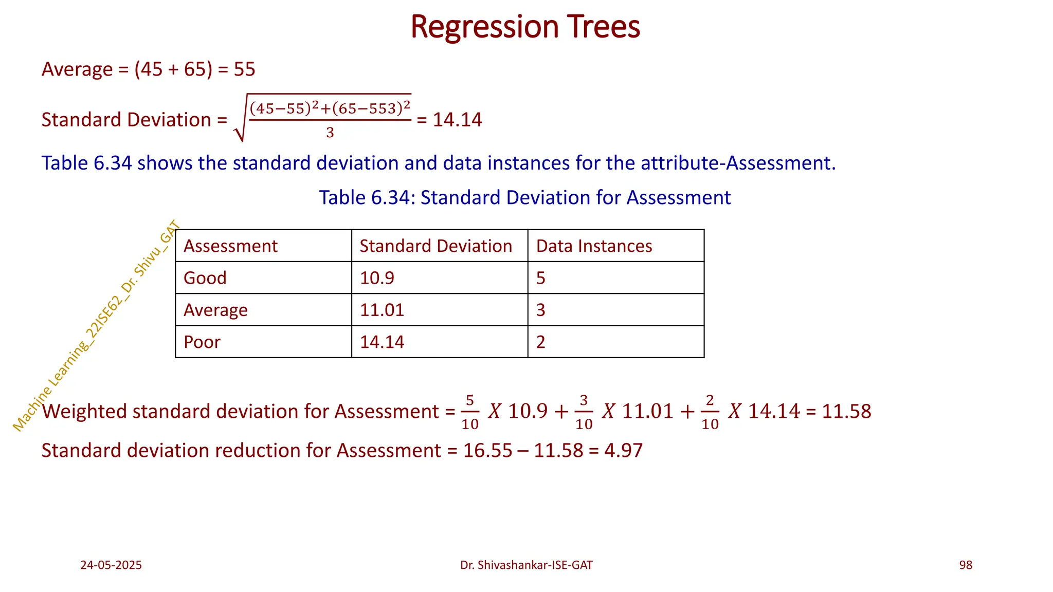
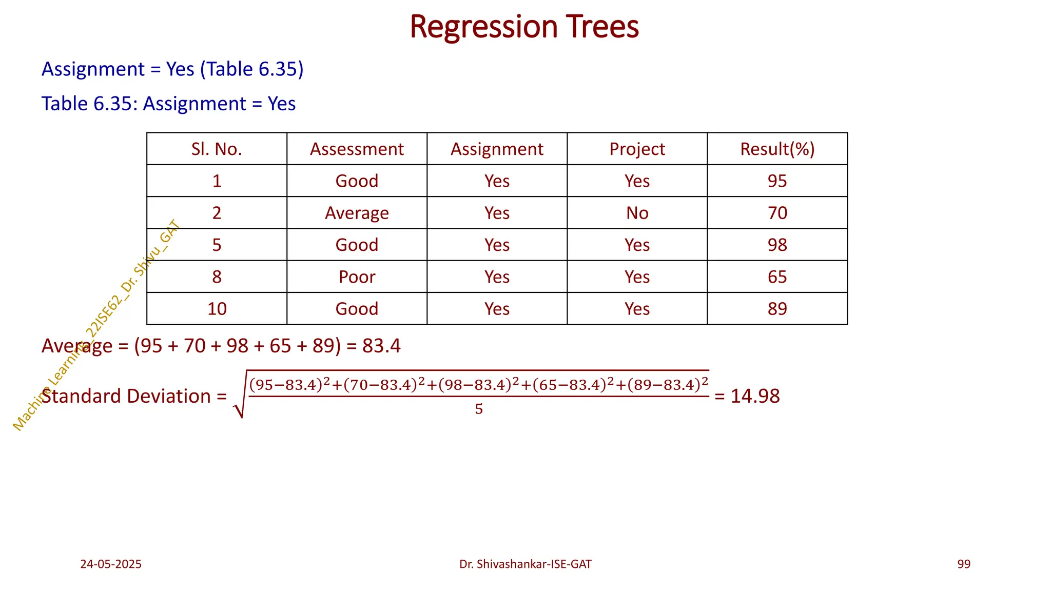
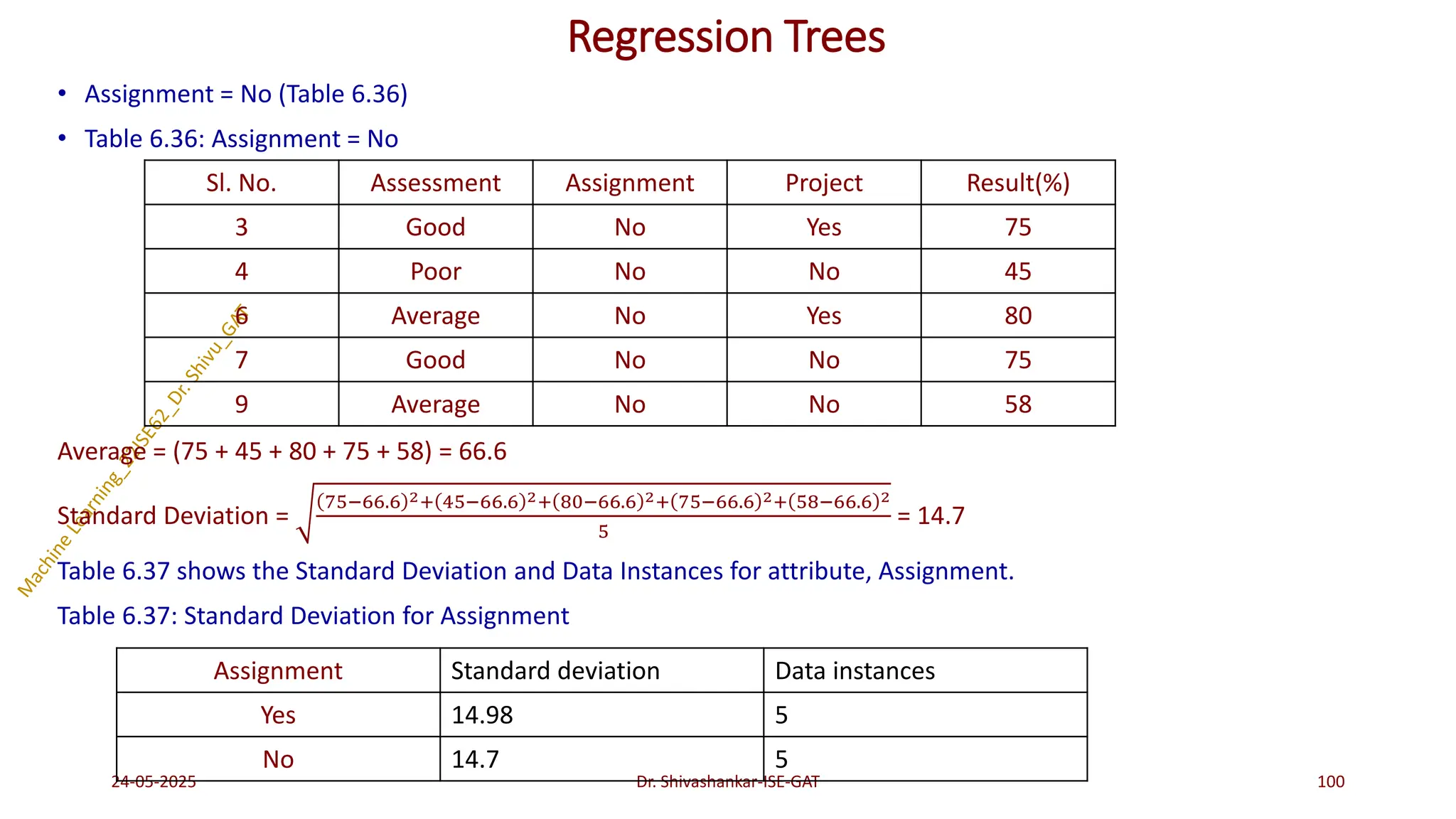
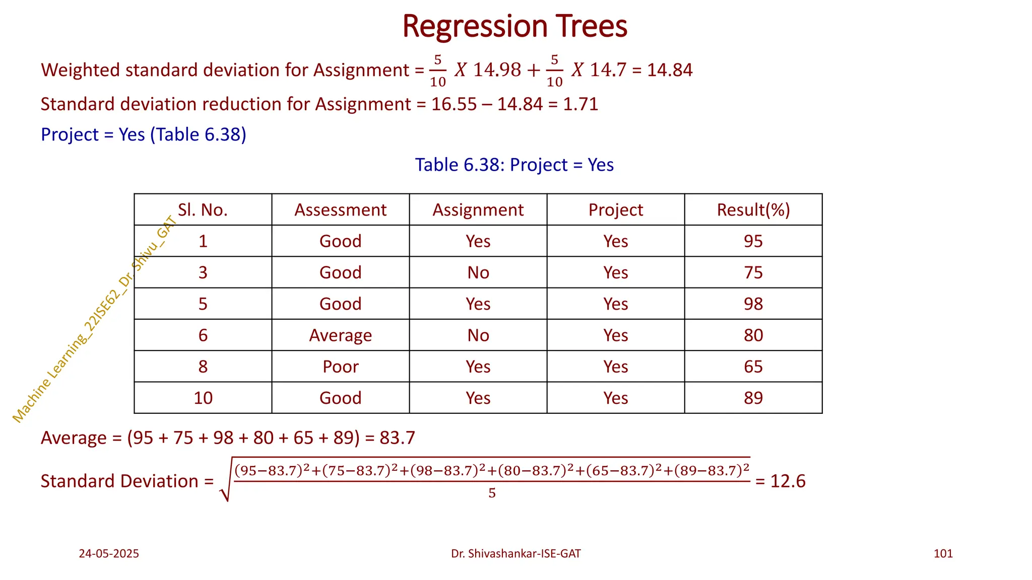
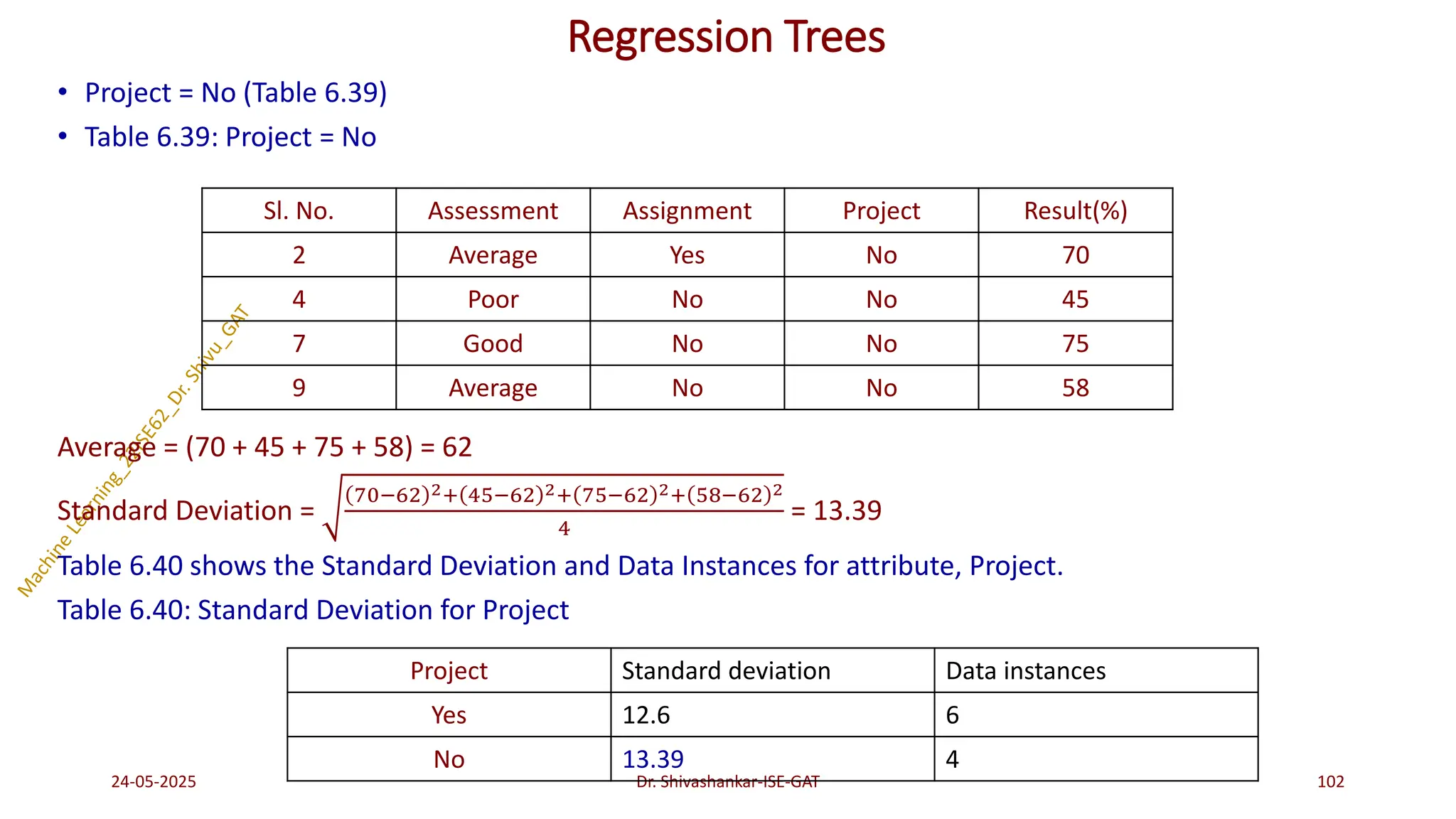
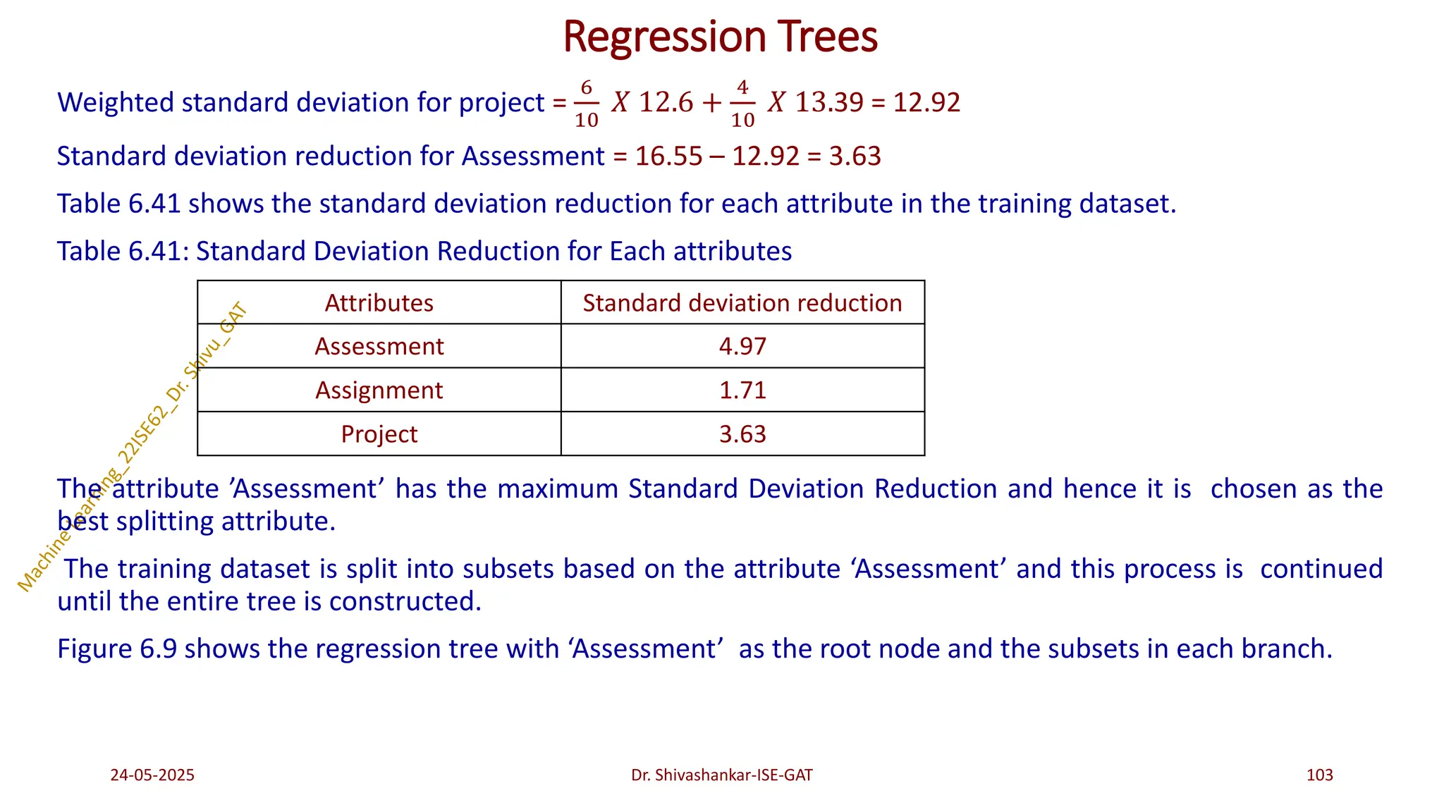
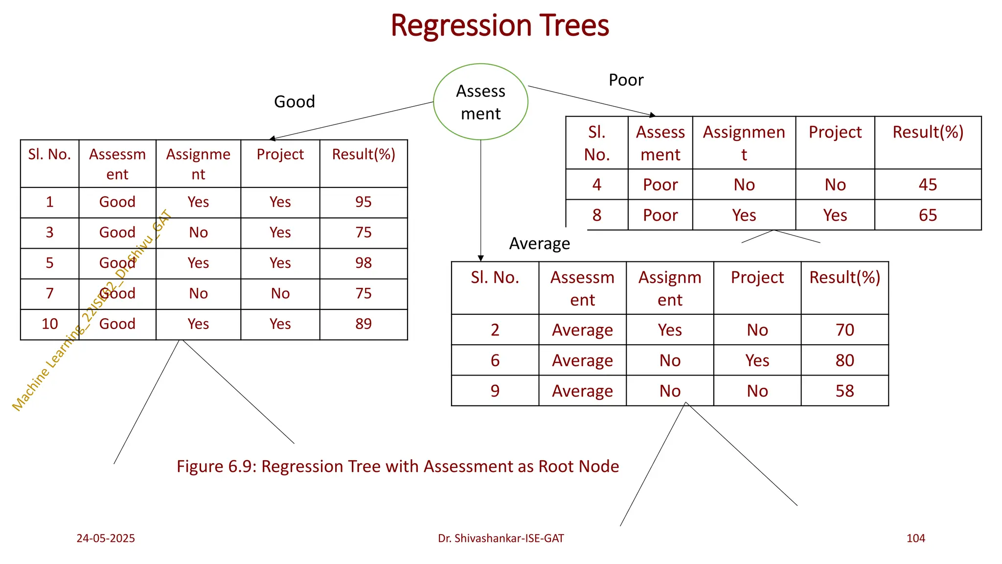


![Conti..
Centroid of class ‘A’ = (3 + 5 + 4, 1 + 2 + 3)/3 = (12, 6)/3 = (4, 2)
Centroid of class ‘B’ = (7 + 6 + 8, 6 + 7 + 5)/3 = (21, 18)/3 = (7, 6)
Now given a test instance (6, 5), we can predict the class.
Step 2: Calculate the Euclidean distance between test instance (6, 5) and each of the centroid.
Euc_Dist[(6, 5); (4, 2)] = 6 − 4 2 + 5 − 2 2= 3.6
Euc_Dist[(6, 5); (7, 6)] = 6 − 7 2 + 5 − 6 2= 1.414
The test instance has smaller distance to class B. Hence, the class of this test instance is predicted as ‘B’.
24-05-2025 21
Dr. Shivashankar-ISE-GAT](https://crownmelresort.com/image.slidesharecdn.com/machinelearning-module3-250524092052-1361b02d/75/Dr-Shivu__Machine-Learning-Module-3-pdf-21-2048.jpg)


![Conti..
Instances 2, 3 and 4 are closer with smaller distances. The mean value = (5 + 7 + 8)/3 =
20/3 = 6.67. Compute the weights for the closest instances, using the Gaussian kernel
𝑤𝑖=exp −
𝑥𝑖−𝑥 2
2𝜏2
Weight of Instance 2:
𝑤2=exp −
𝑥2−𝑥 2
2𝜏2 = exp −
1−2 2
2𝑥0.42 = 𝑒−3.125= 0.043
Weight of Instance 3:
𝑤3=exp −
𝑥3−𝑥 2
2𝜏2 = exp −
2−2 2
2𝑥0.42 = 𝑒0= 1
Weight of Instance 4:
𝑤4=exp −
𝑥4−𝑥 2
2𝜏2 = exp −
1−2 2
2𝑥0.42 = 𝑒−3.125= 0.043
𝑒0
= 1 [𝑤3 is closer hence gets a higher weight value]
24-05-2025 25
Dr. Shivashankar-ISE-GAT](https://crownmelresort.com/image.slidesharecdn.com/machinelearning-module3-250524092052-1361b02d/75/Dr-Shivu__Machine-Learning-Module-3-pdf-25-2048.jpg)


![Conti..
Problem 1: Find linear regression of the data of week and product sales (in Thousands). Use linear regression
in matrix form.
Table 5.3: Sample Data for Regression
Solution: Solution: The dependent variable X is be given as: 𝑥𝑇 = [1 2 3 4]
And the independent variable is given as follows: 𝑦𝑇 = [1 3 4 8]
The data can be given in matrix form as follows: X
1 1
1 2
1 3
1 4
and Y=
1
3
4
8
24-05-2025 42
Dr. Shivashankar-ISE-GAT
𝑥𝑖
Week
𝑦𝑖
Product Sales in Thousands
1 1
2 3
3 4
4 8](https://crownmelresort.com/image.slidesharecdn.com/machinelearning-module3-250524092052-1361b02d/75/Dr-Shivu__Machine-Learning-Module-3-pdf-42-2048.jpg)


![Conti..
Let P be the probability distribution of data instances from 1 to n.
So, P = 𝑃1, 𝑃2, … … 𝑃𝑛
Entropy of P is the information measure of this probability distribution given as,
Entropy_Info(P) = Entropy_Info (𝑃1, 𝑃2, … … 𝑃𝑛) = -(𝑃1𝑙𝑜𝑔2𝑃1+𝑃2𝑙𝑜𝑔2𝑃2 +…..+𝑃𝑛𝑙𝑜𝑔2𝑃𝑛)
where, 𝑃1 is the probability of data instances classified as class 1 and 𝑃2 is the probability
of data instances classified as class 2 and so on.
𝑃1 =
|𝑁𝑜 𝑜𝑓 𝑑𝑎𝑡𝑎 𝑖𝑛𝑠𝑡𝑎𝑛𝑐𝑒𝑠 𝑏𝑒𝑙𝑜𝑛𝑔𝑖𝑛𝑔 𝑡𝑜 𝑐𝑙𝑎𝑠𝑠 1|
|𝑇𝑜𝑡𝑎𝑙 𝑛𝑜 𝑜𝑓 𝑑𝑎𝑡𝑎 𝑖𝑛𝑠𝑡𝑎𝑛𝑐𝑒𝑠 𝑖𝑛 𝑡ℎ𝑒 𝑡𝑟𝑎𝑖𝑛𝑖𝑛𝑔 𝑑𝑎𝑡𝑎𝑠𝑒𝑡|
Mathematically, entropy is defined as
Entropy_Info(X) = σ𝑥𝜖𝑣𝑎𝑙𝑢𝑒𝑠(𝑋) 𝑝𝑟 𝑋 = 𝑥 . 𝑙𝑜𝑔2
1
𝑝𝑟 𝑋=𝑥 .
Pr[X = x] is the probability of a random variable X with a possible outcome x.
24-05-2025 66
Dr. Shivashankar-ISE-GAT](https://crownmelresort.com/image.slidesharecdn.com/machinelearning-module3-250524092052-1361b02d/75/Dr-Shivu__Machine-Learning-Module-3-pdf-66-2048.jpg)


![Conti..
Solution:
Step 1: Calculate the Entropy for the target class ‛Job Offer’.
Entropy_Info(Target Attribute = Job Offer) = Entropy_Info(7, 3) = -[
7
10
𝑙𝑜𝑔2
7
10
+
3
10
𝑙𝑜𝑔2
3
10
] = -(-0.3602 + -0.5210) =
0.8812
Iteration 1:
Step 2: Calculate the Entropy_Info and Gain(Information_Gain) for each of the attribute in the training dataset.
Table 6.4 shows the number of data instances classified with Job Offer as Yes or No for the attribute CGPA.
Table 6.4: Entropy Information for CGPA CGPA
Entropy_Info(T, CGPA) =
4
10
[−
3
4
𝑙𝑜𝑔2
3
4
−
1
4
𝑙𝑜𝑔2
1
4
] +
4
10
[−
4
4
𝑙𝑜𝑔2
4
4
−
0
4
𝑙𝑜𝑔2
0
4
] +
2
10
[−
0
2
𝑙𝑜𝑔2
0
2
−
2
2
𝑙𝑜𝑔2
2
2
] = 0.3243
Gain (CGPA) = Entropy_Info(Target Attribute = Job Offer) - Entropy_Info(T, CGPA) = 0.8812 - 0.3245 = 0.5567
24-05-2025 72
Dr. Shivashankar-ISE-GAT
CGPA Job offer = Yes Job offer = No Total Entropy
≥ 9 3 1 4
≥ 8 4 0 4 0
<8 0 2 2 0](https://crownmelresort.com/image.slidesharecdn.com/machinelearning-module3-250524092052-1361b02d/75/Dr-Shivu__Machine-Learning-Module-3-pdf-72-2048.jpg)
![Conti..
Table 6.5 shows the number of data instances classified with Job Offer as Yes or No for the attribute
Interactiveness.
Table 6.5: Entropy Information for Interactiveness.
Entropy_Info(T, Interactiveness) =
6
10
[−
5
6
𝑙𝑜𝑔2
5
6
−
1
6
𝑙𝑜𝑔2
1
6
] +
4
10
[−
2
4
𝑙𝑜𝑔2
2
4
− −
2
4
𝑙𝑜𝑔2
2
4
] = 0.7896
Gain(Interactiveness) = Entropy_Info(Target Attribute = Job Offer) - Entropy_Info(T, Interactiveness) = 0.8807
- 0.7896 = 0.0911
Table 6.6 shows the number of data instances classified with Job Offer as Yes or No for the attribute
Practical Knowledge. Table 6.6: Entropy Information for Practical Knowledge
24-05-2025 73
Dr. Shivashankar-ISE-GAT
Interactiveness Job offer = Yes Job offer = No Total Entropy
Yes 5 1 6
No 2 2 4
Practical
knowledge
Job offer = Yes Job offer = No Total Entropy
Very good 2 0 2 0
Good 1 2 3
Average 4 1 5](https://crownmelresort.com/image.slidesharecdn.com/machinelearning-module3-250524092052-1361b02d/75/Dr-Shivu__Machine-Learning-Module-3-pdf-73-2048.jpg)
![Conti..
Entropy_Info(T, Practical Knowledge) =
2
10
[−
2
2
𝑙𝑜𝑔2
2
2
−
0
2
𝑙𝑜𝑔2
0
2
] +
3
10
[−
1
3
𝑙𝑜𝑔2
1
3
−
2
3
𝑙𝑜𝑔2
2
3
] +
5
10
[−
4
5
𝑙𝑜𝑔2
4
5
−
−
1
5
𝑙𝑜𝑔2
1
5
] = 0.6361
Gain(Practical Knowledge) = Entropy_Info(Target Attribute = Job Offer) - Entropy_Info(T, Practical Knowledge) =
0.8807 - 0.6361 = 0.2446
Table 6.7 shows the number of data instances classified with Job Offer as Yes or No for the attribute
Communication Skills. Table 6.7: Entropy Information for Communication Skills
Entropy_Info(T, Communication Skills) =
5
10
[−
4
5
𝑙𝑜𝑔2
4
5
−
1
5
𝑙𝑜𝑔2
1
5
] +
3
10
[−
3
3
𝑙𝑜𝑔2
3
3
− −
0
3
𝑙𝑜𝑔2
0
3
] +
2
10
[−
0
2
𝑙𝑜𝑔2
0
2
−
2
2
𝑙𝑜𝑔2
2
2
] = 0.3609
Gain(Communication Skills) = Entropy_Info(Target Attribute = Job Offer) - Entropy_Info(T, Communication Skills) =
0.8813 - 0.36096 = 0.5203
24-05-2025 74
Dr. Shivashankar-ISE-GAT
Communication Skill Job offer = Yes Job offer = No Total
Good 4 1 5
Moderate 3 0 3
Poor 0 2 2](https://crownmelresort.com/image.slidesharecdn.com/machinelearning-module3-250524092052-1361b02d/75/Dr-Shivu__Machine-Learning-Module-3-pdf-74-2048.jpg)

![Conti..
Now, continue the same process for the subset of data instances branched with CGPA ≥ 9 (Highest attributes)
Iteration 2: In this iteration, the same process of computing the Entropy_Info and Gain are repeated with the
subset of training set. Job Offer has 3 instances as Yes and 1 instance as No.
Entropy_Info(T) = Entropy_Info(3, 1) = - [
3
4
𝑙𝑜𝑔2
3
4
+
1
4
𝑙𝑜𝑔2
1
4
] = 0.8112
Entropy_Info(T, Interactiveness) =
2
4
[−
2
2
𝑙𝑜𝑔2
2
2
−
0
2
𝑙𝑜𝑔2
0
2
] +
2
4
[−
1
2
𝑙𝑜𝑔2
1
2
−
1
2
𝑙𝑜𝑔2
1
2
] = 0.4997
Gain(Interactiveness) = 0.8112 - 0.4997 = 0.3115
Entropy_Info(T, Practical Knowledge) =
2
4
[−
2
2
𝑙𝑜𝑔2
2
2
−
0
2
𝑙𝑜𝑔2
0
2
] +
1
4
[−
1
1
𝑙𝑜𝑔2
1
1
−
1
1
𝑙𝑜𝑔2
1
1
] +
1
4
[−
1
1
𝑙𝑜𝑔2
1
1
−
1
1
𝑙𝑜𝑔2
1
1
] = 0
Gain(Practical Knowledge) = 0.8112
Entropy_Info(T, Communication Skills) =
2
4
[−
2
2
𝑙𝑜𝑔2
2
2
−
0
2
𝑙𝑜𝑔2
0
2
] +
1
4
[−
1
1
𝑙𝑜𝑔2
1
1
−
1
1
𝑙𝑜𝑔2
1
1
] +
1
4
[−
1
1
𝑙𝑜𝑔2
1
1
−
1
1
𝑙𝑜𝑔2
1
1
] = 0
Gain (Communication Skills) = 0.8112
The gain calculated for all the attributes is shown in Table 6.9.
24-05-2025 76
Dr. Shivashankar-ISE-GAT
Attributes Gain
Interactiveness 0.3111
Practical knowledge 0.8112
Communication skill 0.8112
Interactiveness Job offer=Yes Job Offer = No
Yes 2 0
No 1 1](https://crownmelresort.com/image.slidesharecdn.com/machinelearning-module3-250524092052-1361b02d/75/Dr-Shivu__Machine-Learning-Module-3-pdf-76-2048.jpg)

![Problems
Problem 1: Construct decision tree using ID3, considering the following example.
Solution:
Attribute : a1
Values(a1)=True / False
S=[6+,4-], Entropy (S)= -
6
10
log2
6
10
−
4
10
log2
4
10
= 0.9709
𝑆𝑇𝑟𝑢𝑒=[1+,4-], Entropy (𝑆𝑇𝑟𝑢𝑒)= -
1
5
log2
1
5
−
4
5
log2
4
5
= 0.7219
𝑆𝐹𝑎𝑙𝑠𝑒=[5+,0-], Entropy (𝑆𝐹𝑎𝑙𝑠𝑒)= -
5
5
log2
5
5
−
0
5
log2
0
5
= 0.0
Gain (S,a1)= Entropy (S) - σ𝑣𝜖{𝑇𝑟𝑢𝑒𝑠,𝑓𝑎𝑙𝑠𝑒}
𝑆𝑣
𝑆
𝐸𝑛𝑡𝑟𝑜𝑝𝑦(𝑆𝑣)
Gain (S,a1)=Entropy (S) -
5
10
Entropy (𝑆𝑇𝑟𝑢𝑒) -
5
10
Entropy (𝑆𝐹𝑎𝑙𝑠𝑒)
= 0.9709 -
5
10
X0.7219 -
5
10
X0.0= 0.6099
5/24/2025 78
Dr. Shivashankar, ISE, GAT
Instance a1 a2 a3 Classifi
cation
1 True Hot High No
2 True Hot High No
3 False Hot High Yes
4 False Cool Normal Yes
5 False Cool Normal Yes
6 True Cool High No
7 True Hot High No
8 True Hot Normal Yes
9 False Cool Normal Yes
10 False Cool High Yes
Yes No
Yes No](https://crownmelresort.com/image.slidesharecdn.com/machinelearning-module3-250524092052-1361b02d/75/Dr-Shivu__Machine-Learning-Module-3-pdf-78-2048.jpg)
![Cont…
Attribute : a2
Values(a2)=Hot, Cool
S=[6+,4-], Entropy (S)= -
6
10
log2
6
10
−
4
10
log2
4
10
= 0.9709
𝑆𝐻𝑜𝑡=[2+, 3-], Entropy (𝑆𝐻𝑜𝑡)= -
2
5
log2
2
5
−
3
5
log2
3
5
= 0.9709
𝑆𝐶𝑜𝑜𝑙=[4+,1-], Entropy (𝑆𝐶𝑜𝑜𝑙)= -
4
5
log2
4
5
−
1
5
log2
1
5
= 0.7219
Gain (S,a2)= Entropy (S) - σ𝑣𝜖{𝐻𝑜𝑡,𝐶𝑜𝑜𝑙}
𝑆𝑣
𝑆
𝐸𝑛𝑡𝑟𝑜𝑝𝑦(𝑆𝑣)
Gain (S,a2)=Entropy (S) -
5
10
Entropy (𝑆𝐻𝑜𝑡) -
5
10
Entropy (𝑆𝐶𝑜𝑜𝑙)
= 0.9709 -
5
10
X0.9709 -
5
10
X0.7219= 0.1245
Attribute : a3
Values(a3)=High, Normal
S=[6+,4-] Entropy (S)= -
6
10
log2
6
10
−
4
10
log2
4
10
= 0.9709
𝑆𝐻𝑖𝑔ℎ=[2+, 4-] Entropy (𝑆𝐻𝑖𝑔ℎ)= -
2
6
log2
2
6
−
4
5
log2
4
5
= 0.9183
𝑆𝑁𝑜𝑟𝑚𝑎𝑙=[4+,0-] Entropy (𝑆𝑁𝑜𝑟𝑚𝑎𝑙)= -
4
4
log2
4
4
−
0
4
log2
0
4
= 0.0
Gain (S,a3)= Entropy (S) - σ𝑣𝜖{𝐻𝑖𝑔ℎ,𝑁𝑜𝑟𝑚𝑎𝑙}
𝑆𝑣
𝑆
𝐸𝑛𝑡𝑟𝑜𝑝𝑦(𝑆𝑣)
Gain (S,a3)=Entropy (S) -
6
10
Entropy (𝑆𝐻𝑖𝑔ℎ) −
4
10
Entropy (𝑆𝑁𝑜𝑟𝑚𝑎𝑙) = 0.9709 -
6
10
X0.9183 -
4
10
X0.0
5/24/2025 79
Dr. Shivashankar, ISE, GAT](https://crownmelresort.com/image.slidesharecdn.com/machinelearning-module3-250524092052-1361b02d/75/Dr-Shivu__Machine-Learning-Module-3-pdf-79-2048.jpg)
![Cont…
∴ Gain (S,a1)= 0.6099- Maximum
Gain (S,a2)= 0.1245
Gain (S,a3)= 0.4199
Attribute : a2
Values(a2)=Hot, Cool
𝑆𝑎2=[1+,4-] Entropy (𝑆𝑎2)= -
1
5
log2
1
5
−
4
5
log2
4
5
= 0.7219
𝑆𝐻𝑜𝑡=[1+, 3-] Entropy (𝑆𝐻𝑜𝑡)= -
1
4
log2
1
4
−
3
4
log2
3
4
= 0.8112
𝑆𝐶𝑜𝑜𝑙=[0+,1-] Entropy (𝑆𝐶𝑜𝑜𝑙)= -
0
1
log2
0
1
−
1
1
log2
1
1
= 0.0
Gain (S,a2)= Entropy (S) - σ𝑣𝜖{𝐻𝑜𝑡,𝐶𝑜𝑜𝑙}
𝑆𝑣
𝑆
𝐸𝑛𝑡𝑟𝑜𝑝𝑦(𝑆𝑣)
Gain (S,a2)=Entropy (S) -
4
5
Entropy (𝑆𝐻𝑜𝑡) -
1
5
Entropy (𝑆𝐶𝑜𝑜𝑙)
5/24/2025 80
Dr. Shivashankar, ISE, GAT
a1
True False
1,2,6,7,8 3,4,5,9,10
Yes
Instance a2 a3 Classific
ation
1 Hot High No
2 Hot High No
6 Cool High No
7 Hot High No
8 Hot Normal Yes
?](https://crownmelresort.com/image.slidesharecdn.com/machinelearning-module3-250524092052-1361b02d/75/Dr-Shivu__Machine-Learning-Module-3-pdf-80-2048.jpg)
![Cont…
Attribute : a3
Values(a3)=High, Normal
𝑆𝑎3=[1+,4-] Entropy (𝑆𝑎3)= -
1
5
log2
1
5
−
4
5
log2
4
5
= 0.7219
𝑆𝐻𝑖𝑔ℎ=[0+, 4-] Entropy (𝑆𝐻𝑖𝑔ℎ)= -
0
4
log2
0
4
−
4
4
log2
4
4
= 0.0
𝑆𝑁𝑜𝑟𝑚𝑎𝑙=[1+,0-] Entropy (𝑆𝑁𝑜𝑟𝑚𝑎𝑙)= -
1
1
log2
1
1
−
0
1
log2
0
1
= 0.0
Gain (S,a3)= Entropy (S) - σ𝑣𝜖{𝐻𝑖𝑔ℎ,𝑁𝑜𝑟𝑚𝑎𝑙}
𝑆𝑣
𝑆
𝐸𝑛𝑡𝑟𝑜𝑝𝑦(𝑆𝑣)
Gain (S,a3)=Entropy (S) -
4
5
Entropy (𝑆𝐻𝑖𝑔ℎ) -
1
5
Entropy (𝑆𝑁𝑜𝑟𝑚𝑎𝑙) = 0.9709 -
4
5
X0.0 -
1
5
X0.0
= 0.9709
∴ Gain (Sa1,a2)=0.3210
Gain(Sa1, a3)=0.9709---Maximum
5/24/2025 81
Dr. Shivashankar, ISE, GAT
a1
True False
1,2,6,7,8 3,4,5,9,10
a3
1,2,6,7 8
High Normal
Yes
Yes
No](https://crownmelresort.com/image.slidesharecdn.com/machinelearning-module3-250524092052-1361b02d/75/Dr-Shivu__Machine-Learning-Module-3-pdf-81-2048.jpg)


![Conti..
Example 6.4: Make use of Information Gain of the attributes which are calculated in ID3 algorithm in
Example 6.3 to construct a decision tree using C4.5.
Solution: Iteration 1:
Step 1: Calculate the Class_Entropy for the target class ‘Job Offer’. Entropy_Info(Target Attribute = Job Offer)
= Entropy_Info(7, 3) = −[
7
10
𝑙𝑜𝑔2
7
10
+
3
10
𝑙𝑜𝑔2
3
10
] = 0.8807
Step 2: Calculate the Entropy_Info, Gain(Info_Gain), Split_Info, Gain_Ratio for each of the attribute in the
training dataset.
CGPA:
Entropy Info(T, CGPA) =
4
10
[−
3
4
𝑙𝑜𝑔2
3
4
−
1
4
𝑙𝑜𝑔2
1
4
] +
4
10
[−
4
4
𝑙𝑜𝑔2
4
4
−
0
4
𝑙𝑜𝑔2
0
4
] +
2
10
[−
0
2
𝑙𝑜𝑔2
0
2
−
2
2
𝑙𝑜𝑔2
2
2
] =
0.3243
Gain(CGPA) = 0.8807 - 0.3243 = 0.5564
Split _ Info(, CGPA) = −
4
10
𝑙𝑜𝑔2
4
10
−
4
10
𝑙𝑜𝑔2
4
10
−
2
10
𝑙𝑜𝑔2
2
10
= 1.5211
Gain Ratio(CGPA) =
(Gain(CGPA))
Split_Info(T, CGPA))
=
0.5564
1.5211
= 0.3658
24-05-2025 85
Dr. Shivashankar-ISE-GAT
CGPA ≥ 9 = 4, ≥ 8 = 4, < 8 = 2](https://crownmelresort.com/image.slidesharecdn.com/machinelearning-module3-250524092052-1361b02d/75/Dr-Shivu__Machine-Learning-Module-3-pdf-85-2048.jpg)
![Conti..
Interactiveness: Entropy Info(T, Interactiveness) =
6
10
[−
5
6
𝑙𝑜𝑔2
5
6
−
1
6
𝑙𝑜𝑔2
1
6
] +
4
10
[−
2
4
𝑙𝑜𝑔2
2
4
−
2
4
𝑙𝑜𝑔2
2
4
] =
0.7896
Gain(Interactiveness) = 0.8807 - 0.7896 = 0.0911
Split _ Info(T, Interactiveness) = −
6
10
𝑙𝑜𝑔2
6
10
−
4
10
𝑙𝑜𝑔2
4
10
= 0.9704
Gain_Ratio(Interactiveness) =
Gain(Interactiveness)
Split _ Info(, Interactiveness)
=
0.0911
0.9704
= 0.0939
Practical Knowledge:
Entropy_Info(T, Practical Knowledge) =
2
10
[−
2
2
𝑙𝑜𝑔2
2
2
−
0
2
𝑙𝑜𝑔2
0
2
] +
3
10
[−
1
3
𝑙𝑜𝑔2
1
3
−
2
3
𝑙𝑜𝑔2
2
3
] +
5
10
[−
4
5
𝑙𝑜𝑔2
4
5
−
1
5
𝑙𝑜𝑔2
1
5
] = 0.6361
Gain(Practical Knowledge) = 0.8807 - 0.6361 = 0.2448
Split_Info(T, Practical Knowledge) = −
2
10
𝑙𝑜𝑔2
2
10
−
5
10
𝑙𝑜𝑔2
5
10
−
3
10
𝑙𝑜𝑔2
3
10
= 1.4853
Gain_Ratio(Practical Knowledge) = −
Gain(Practical Knowledge)
Split _ Info(, Practical Knowledge)
=
0.2448
1.4853
= 0.1648
24-05-2025 86
Dr. Shivashankar-ISE-GAT](https://crownmelresort.com/image.slidesharecdn.com/machinelearning-module3-250524092052-1361b02d/75/Dr-Shivu__Machine-Learning-Module-3-pdf-86-2048.jpg)
![Conti..
Communication Skills:
Entropy_Info(T, Communication Skills) =
5
10
[−
4
5
𝑙𝑜𝑔2
4
5
−
1
5
𝑙𝑜𝑔2
1
5
] +
3
10
[−
3
3
𝑙𝑜𝑔2
3
3
−
0
3
𝑙𝑜𝑔2
0
3
] +
2
10
[−
0
2
𝑙𝑜𝑔2
0
2
−
2
2
𝑙𝑜𝑔2
2
2
] = 0.3609
Gain(Communication Skills) = 0.8813 - 0.36096 = 0.5202
Split _ Info(T, Communication Skills) = −
5
10
𝑙𝑜𝑔2
5
10
−
3
10
𝑙𝑜𝑔2
3
10
−
2
10
𝑙𝑜𝑔2
2
10
= 1.4853
Gain_Ratio(Communication Skills) =
Gain(Communication Skills)
Split_Info(T, Communication Skills)
=
0.5202
1.4853
= 0.3502
Table 6.10: Gain_Ratio
24-05-2025 87
Dr. Shivashankar-ISE-GAT
Attributes Gain Ratio
CGPA 0.3658
Interactiveness 0.0939
Practical Knowledge 0.1648
Communication skill 0.3502](https://crownmelresort.com/image.slidesharecdn.com/machinelearning-module3-250524092052-1361b02d/75/Dr-Shivu__Machine-Learning-Module-3-pdf-87-2048.jpg)

![Conti..
Iteration 2:
Total Samples: 4 Repeat the same process for this resultant dataset with 4 data instances.
Job Offer has 3 instances as Yes and 1 instance as No.
Entropy_Info(Target Class = Job Offer) = −
3
4
𝑙𝑜𝑔2
3
4
−
1
4
𝑙𝑜𝑔2
1
4
= 0.8112
Interactiveness: Entropy_Info(T, Interactiveness) =
2
4
[−
2
2
𝑙𝑜𝑔2
2
2
−
0
2
𝑙𝑜𝑔2
0
2
] +
2
4
[−
1
2
𝑙𝑜𝑔2
1
2
−
1
2
𝑙𝑜𝑔2
1
2
] = 0.4997
Gain(Interactiveness) = 0.8108 - 0.4997 = 0.3111
Split _ Info(T, Interactiveness) = −
2
4
𝑙𝑜𝑔2
2
4
−
2
4
𝑙𝑜𝑔2
2
4
= 1
Gain_Ratio(Interactiveness) =
𝐺𝑎𝑖𝑛 ( 𝐼𝑛𝑡𝑒𝑟𝑎𝑐𝑡𝑖𝑣𝑒𝑛𝑒𝑠𝑠)
Split _ Info(T, Interactiveness)
=
0.3112
1
= 0.3112
Practical Knowledge:
Entropy_Info(T, Practical Knowledge) =
2
4
[−
2
2
𝑙𝑜𝑔2
2
2
−
0
2
𝑙𝑜𝑔2
0
2
] +
1
4
[−
0
1
𝑙𝑜𝑔2
0
1
−
1
1
𝑙𝑜𝑔2
1
1
] +
1
4
[−
1
1
𝑙𝑜𝑔2
1
1
−
0
1
𝑙𝑜𝑔2
0
1
]
= 0
Gain(Practical Knowledge) = 0.8108
Split_Info(T, Practical Knowledge) = −
2
4
𝑙𝑜𝑔2
2
4
−
1
4
𝑙𝑜𝑔2
1
4
−
1
4
𝑙𝑜𝑔2
1
4
= 1.5
24-05-2025 89
Dr. Shivashankar-ISE-GAT](https://crownmelresort.com/image.slidesharecdn.com/machinelearning-module3-250524092052-1361b02d/75/Dr-Shivu__Machine-Learning-Module-3-pdf-89-2048.jpg)
![Conti..
Gain_Ratio(Practical Knowledge) =
𝐺𝑎𝑖𝑛 ( 𝑝𝑟𝑎𝑐𝑡𝑖𝑐𝑎𝑙 𝑘𝑛𝑜𝑤𝑙𝑒𝑑𝑔𝑒)
Split _ Info(T, 𝑝𝑟𝑎𝑐𝑡𝑖𝑐𝑎𝑙 𝑘𝑛𝑜𝑤𝑙𝑒𝑑𝑔𝑒)
=
0.8108
1.5
= 0.5408
Communication Skills: Entropy_Info(T, Communication Skills) =
2
4
[−
2
2
𝑙𝑜𝑔2
2
2
−
0
2
𝑙𝑜𝑔2
0
2
] +
1
4
[−
0
1
𝑙𝑜𝑔2
0
1
−
1
1
𝑙𝑜𝑔2
1
1
] +
1
4
[−
1
1
𝑙𝑜𝑔2
1
1
−
0
1
𝑙𝑜𝑔2
0
1
] =0
Gain(Communication Skills) = 0.8108
Split_Info(T, Practical Knowledge) = −
2
4
𝑙𝑜𝑔2
2
4
−
1
4
𝑙𝑜𝑔2
1
4
−
1
4
𝑙𝑜𝑔2
1
4
= 1.5
Gain_Ratio(Practical Knowledge) =
𝐺𝑎𝑖𝑛 ( 𝐶𝑜𝑚𝑚𝑢𝑛𝑖𝑐𝑎𝑡𝑖𝑜𝑛 𝑠𝑘𝑖𝑙𝑙)
Split _ Info(T, 𝐶𝑜𝑚𝑚𝑢𝑛𝑖𝑐𝑎𝑡𝑖𝑜𝑛 𝑠𝑘𝑖𝑙𝑙)
=
0.8108
1.5
= 0.5408
Table 6.11 shows the Gain_Ratio computed for all the attributes.
Table 6.11: Gain-Ratio Attributes
Both ‘Practical Knowledge’ and ‘Communication Skills’ have the highest gain ratio. So, the best splitting attribute
can either be ‘Practical Knowledge’ or ‘Communication Skills’, and therefore, the split can be based on any one of
these.
24-05-2025 90
Dr. Shivashankar-ISE-GAT
Attributes Gain Ration
Interactiveness 0.3112
Practical Knowledge 0.5408
Communication skill 05408](https://crownmelresort.com/image.slidesharecdn.com/machinelearning-module3-250524092052-1361b02d/75/Dr-Shivu__Machine-Learning-Module-3-pdf-90-2048.jpg)