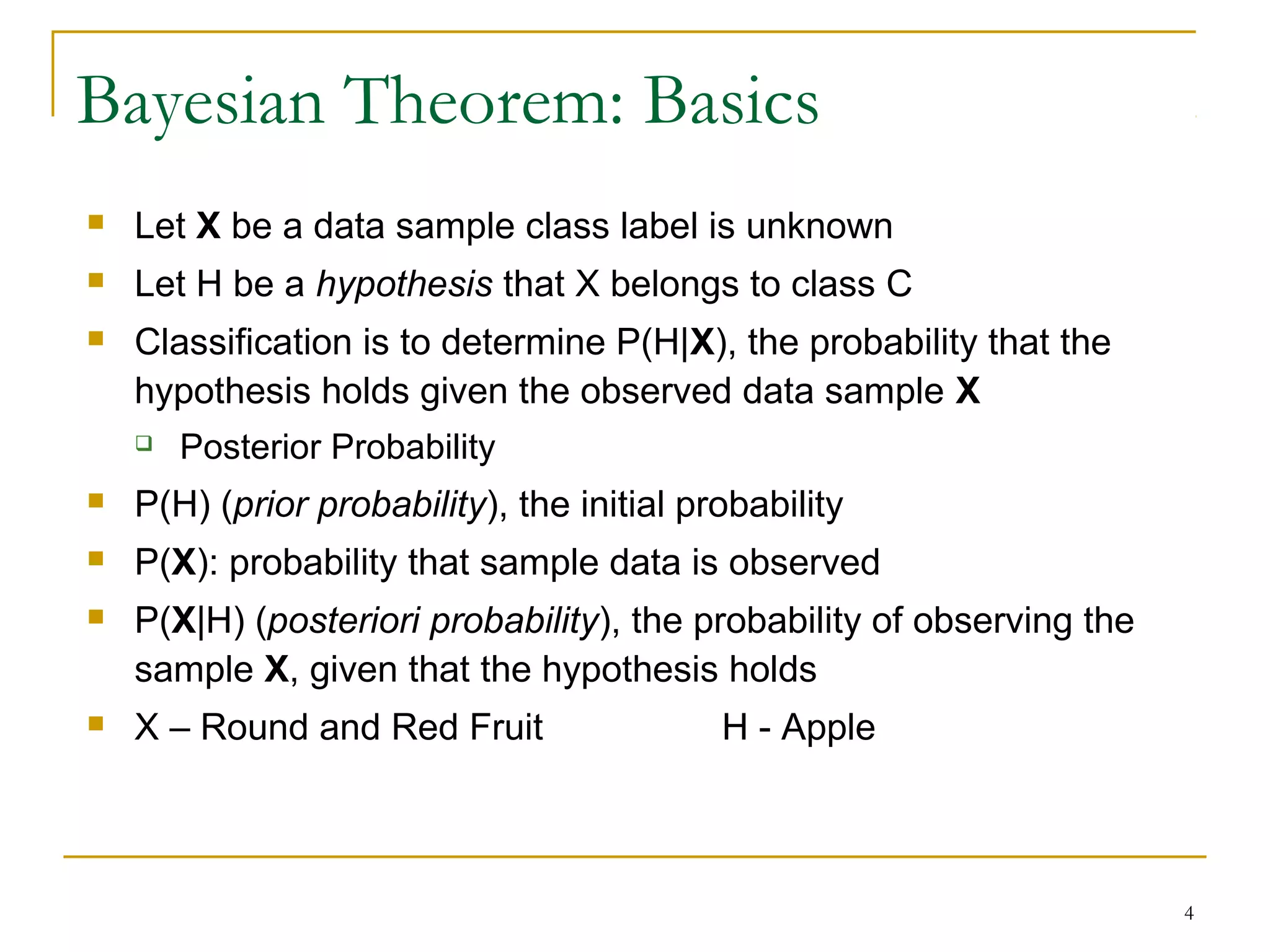
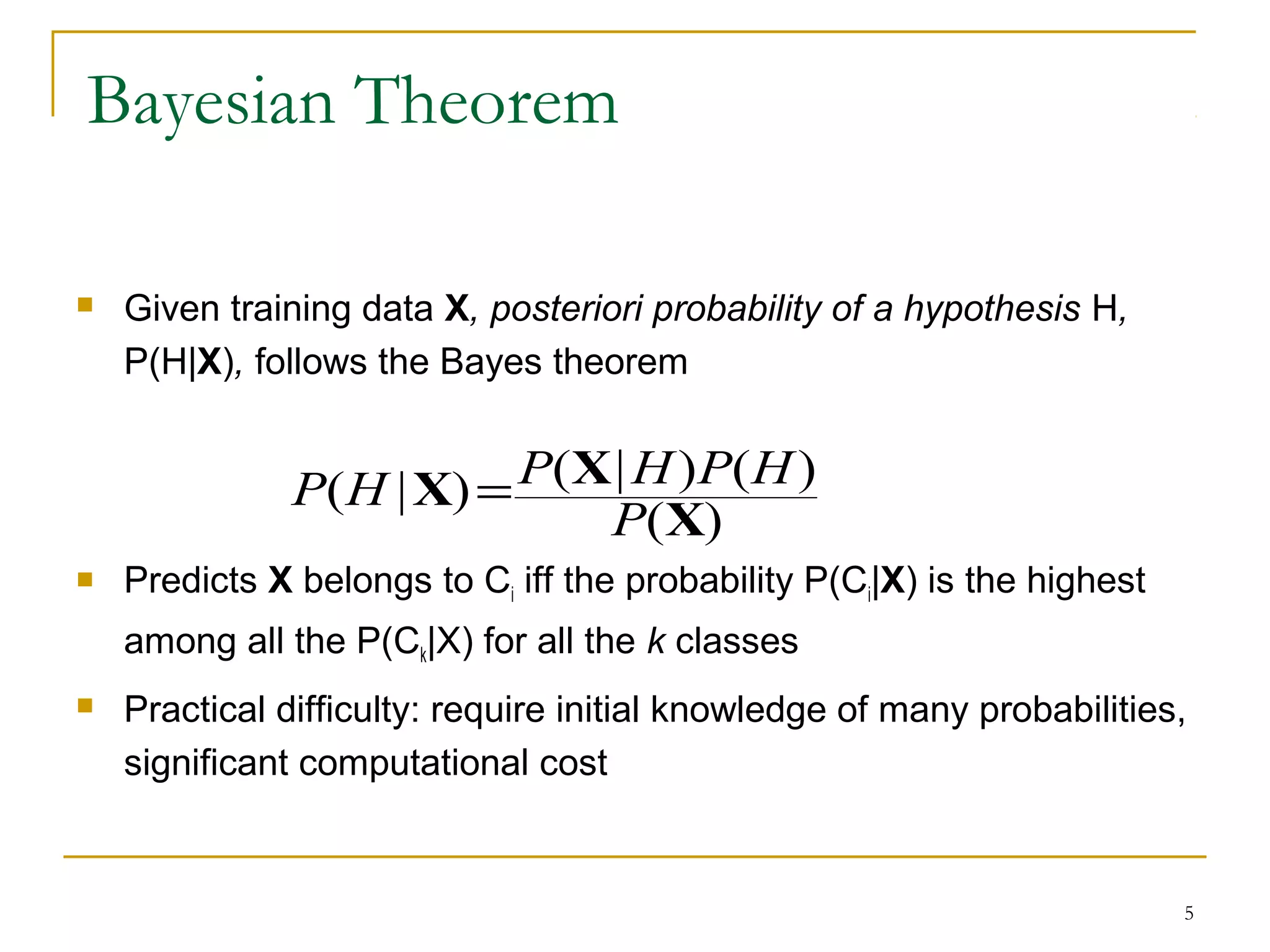
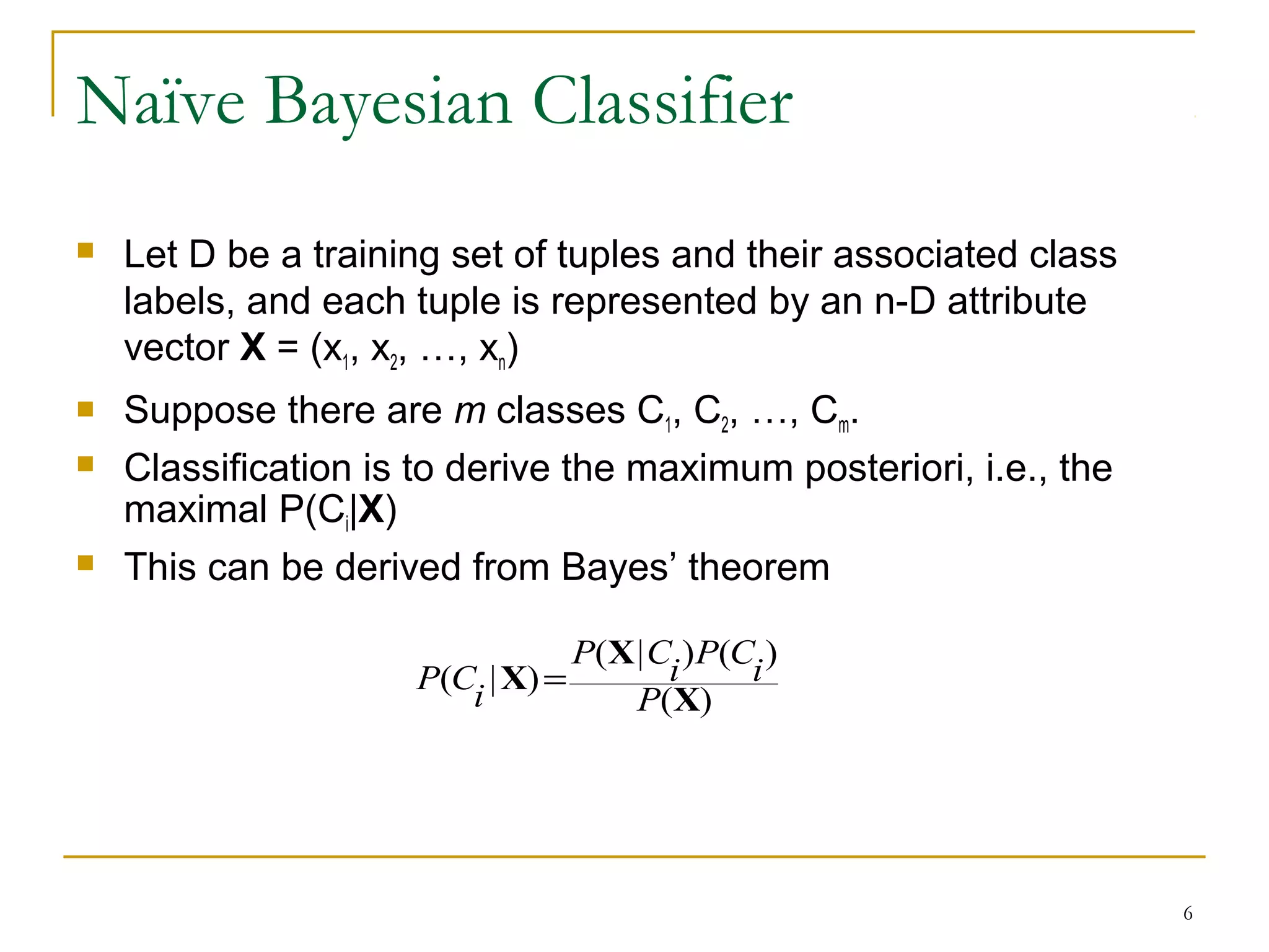
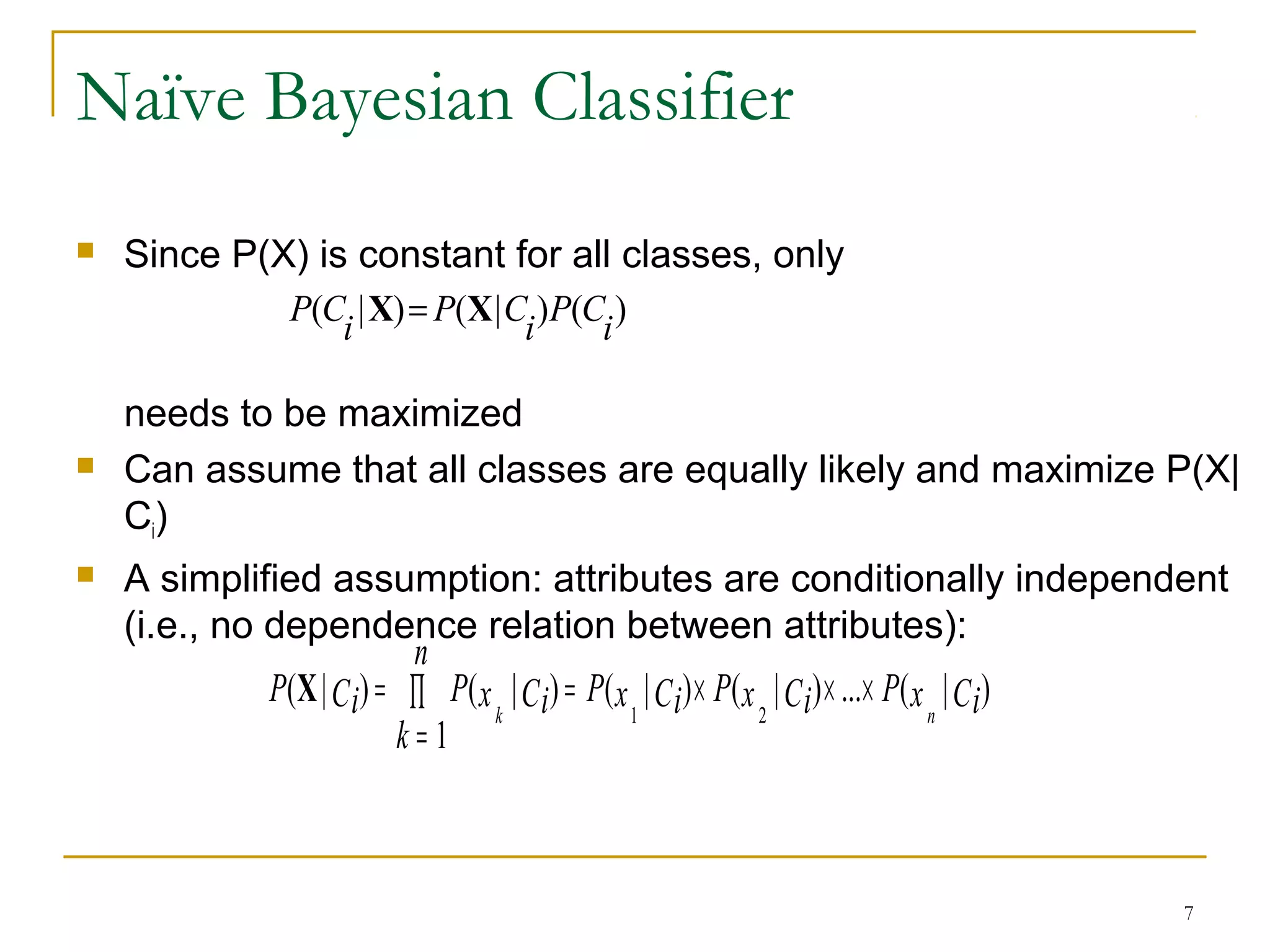
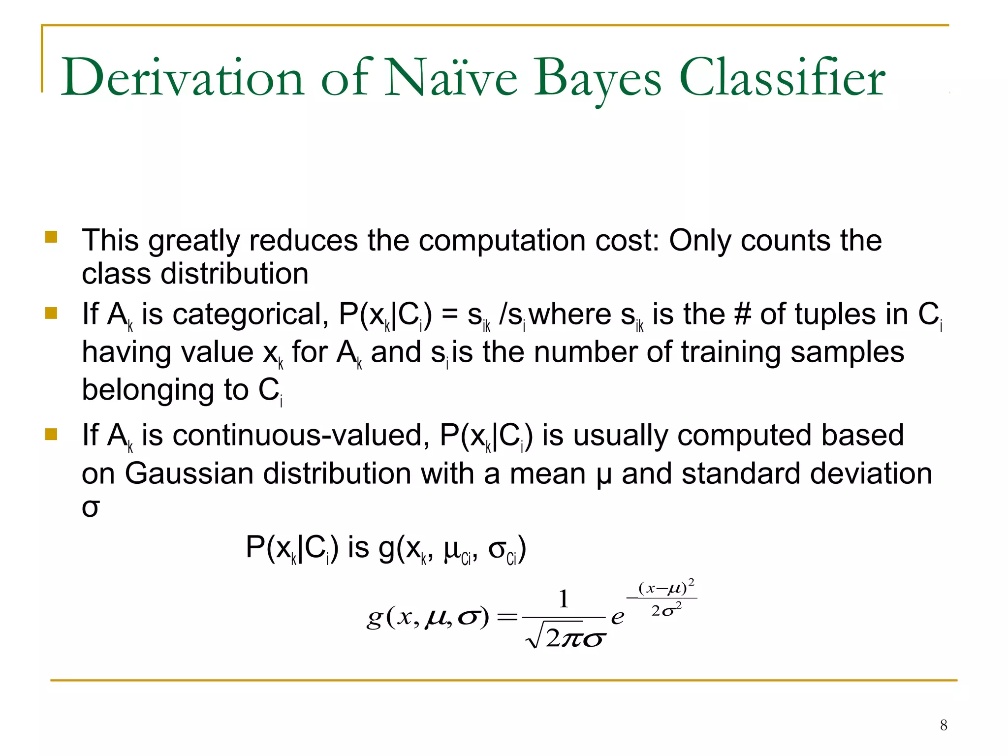
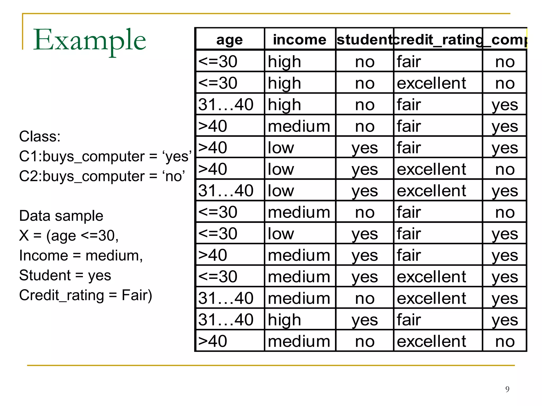
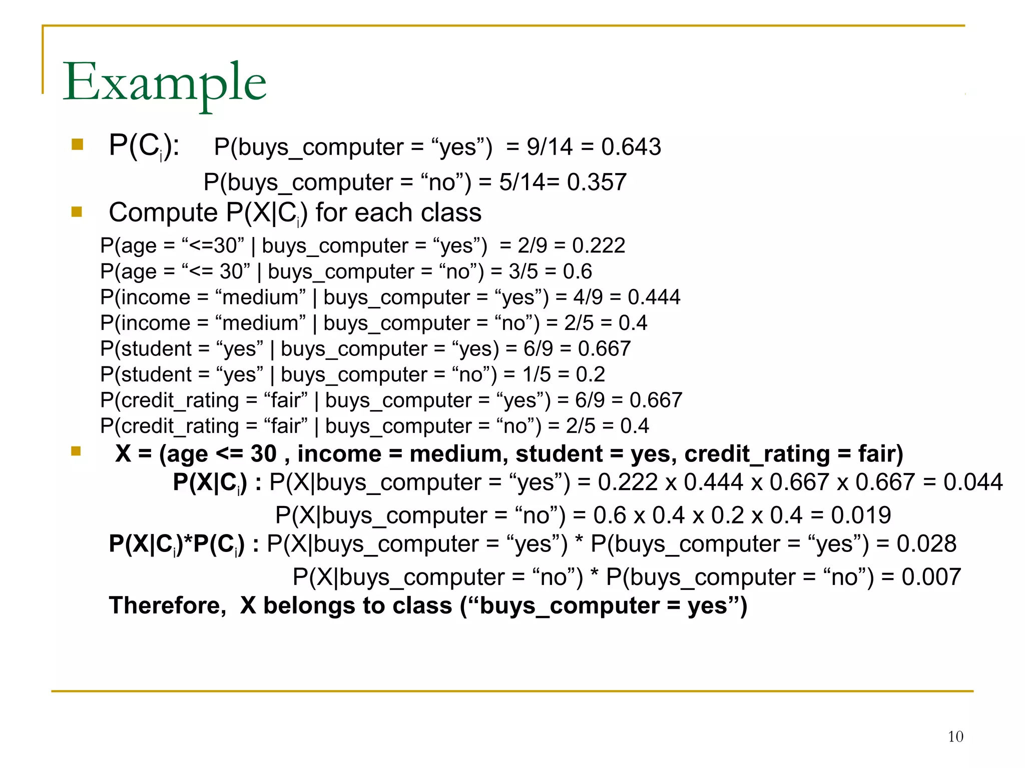
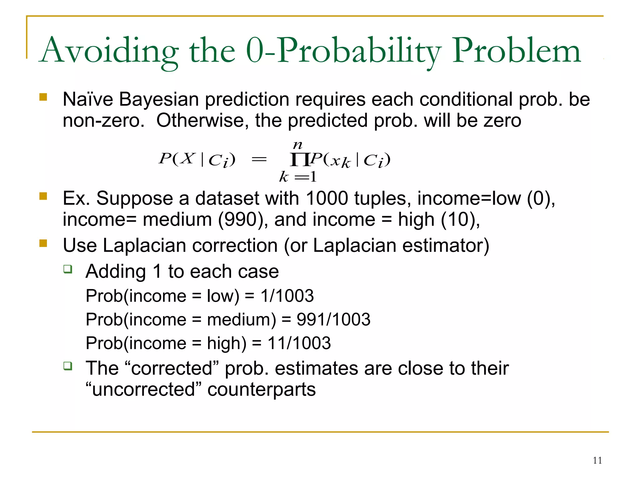
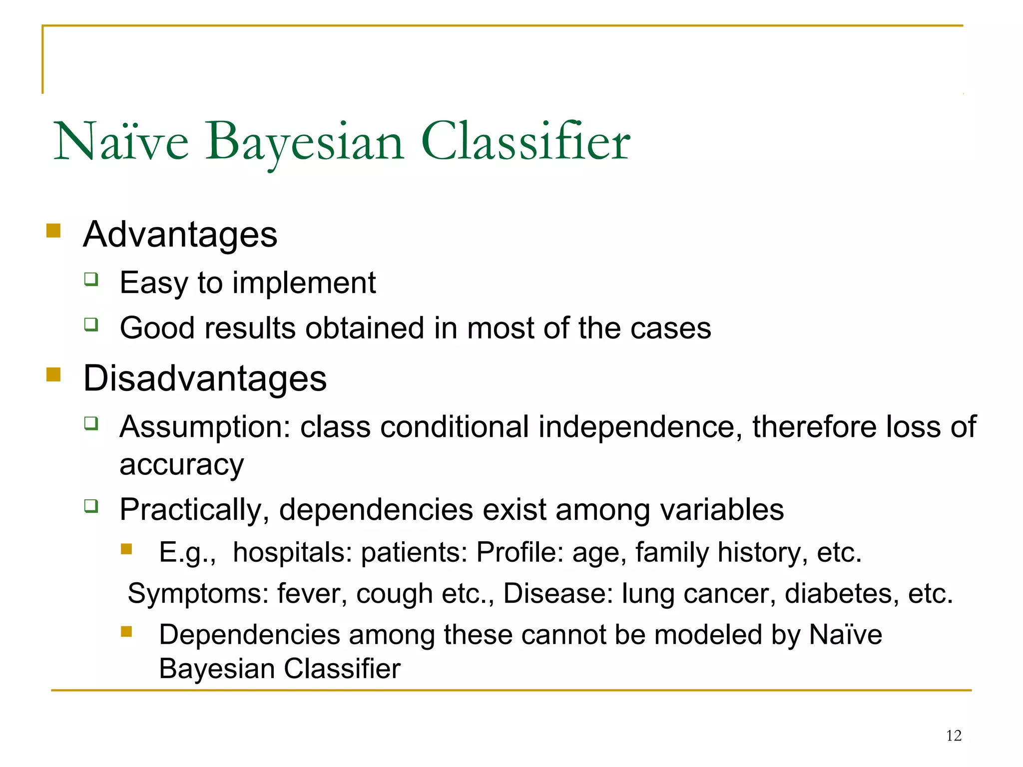
1
Bayesian Classification
2
Bayesian Classification
 A statistical classifier
 Probabilistic prediction
 Predict class membership probabilities
 Based on Bayes’ Theorem
 Naive Bayesian classifier
 comparable performance with decision tree and selected neural
network classifiers
 Accuracy and Speed is good when applied to large databases
 Incremental
3
Bayesian Classification
 Naïve Bayesian Classifier
 Class Conditional Independence
 Effect of an attribute value on a given class is
independent of the values of other attributes
 Simplifies Computations
 Bayesian Belief Networks
 Graphical models
 Represent dependencies among subsets of
attributes
4
Bayesian Theorem: Basics
 Let X be a data sample class label is unknown
 Let H be a hypothesis that X belongs to class C
 Classification is to determine P(H|X), the probability that the
hypothesis holds given the observed data sample X
 Posterior Probability
 P(H) (prior probability), the initial probability
 P(X): probability that sample data is observed
 P(X|H) (posteriori probability), the probability of observing the
sample X, given that the hypothesis holds
 X – Round and Red Fruit H - Apple
5
Bayesian Theorem
 Given training data X, posteriori probability of a hypothesis H,
P(H|X), follows the Bayes theorem
 Predicts X belongs to Ci iff the probability P(Ci|X) is the highest
among all the P(Ck|X) for all the k classes
 Practical difficulty: require initial knowledge of many probabilities,
significant computational cost
)(
)()|()|(
X
XX
P
HPHPHP =
6
Naïve Bayesian Classifier
 Let D be a training set of tuples and their associated class
labels, and each tuple is represented by an n-D attribute
vector X = (x1, x2, …, xn)
 Suppose there are m classes C1, C2, …, Cm.
 Classification is to derive the maximum posteriori, i.e., the
maximal P(Ci|X)
 This can be derived from Bayes’ theorem
)(
)()|(
)|(
X
X
X
P
i
CP
i
CP
i
CP =
7
Naïve Bayesian Classifier
 Since P(X) is constant for all classes, only
needs to be maximized
 Can assume that all classes are equally likely and maximize P(X|
Ci)
 A simplified assumption: attributes are conditionally independent
(i.e., no dependence relation between attributes):
)()|()|(
i
CP
i
CP
i
CP XX =
)|(...)|()|(
1
)|()|(
21
CixPCixPCixP
n
k
CixPCiP
nk
×××=∏
=
=X
8
Derivation of Naïve Bayes Classifier
 This greatly reduces the computation cost: Only counts the
class distribution
 If Ak is categorical, P(xk|Ci) = sik /si where sik is the # of tuples in Ci
having value xk for Ak and si is the number of training samples
belonging to Ci
 If Ak is continuous-valued, P(xk|Ci) is usually computed based
on Gaussian distribution with a mean μ and standard deviation
σ
P(xk|Ci) is g(xk, µCi, σCi)
2
2
2
)(
2
1
),,( σ
µ
σπ
σµ
−
−
=
x
exg
9
Example
Class:
C1:buys_computer = ‘yes’
C2:buys_computer = ‘no’
Data sample
X = (age <=30,
Income = medium,
Student = yes
Credit_rating = Fair)
age income studentcredit_ratingbuys_compu
<=30 high no fair no
<=30 high no excellent no
31…40 high no fair yes
>40 medium no fair yes
>40 low yes fair yes
>40 low yes excellent no
31…40 low yes excellent yes
<=30 medium no fair no
<=30 low yes fair yes
>40 medium yes fair yes
<=30 medium yes excellent yes
31…40 medium no excellent yes
31…40 high yes fair yes
>40 medium no excellent no
10
Example
 P(Ci): P(buys_computer = “yes”) = 9/14 = 0.643
P(buys_computer = “no”) = 5/14= 0.357
 Compute P(X|Ci) for each class
P(age = “<=30” | buys_computer = “yes”) = 2/9 = 0.222
P(age = “<= 30” | buys_computer = “no”) = 3/5 = 0.6
P(income = “medium” | buys_computer = “yes”) = 4/9 = 0.444
P(income = “medium” | buys_computer = “no”) = 2/5 = 0.4
P(student = “yes” | buys_computer = “yes) = 6/9 = 0.667
P(student = “yes” | buys_computer = “no”) = 1/5 = 0.2
P(credit_rating = “fair” | buys_computer = “yes”) = 6/9 = 0.667
P(credit_rating = “fair” | buys_computer = “no”) = 2/5 = 0.4
 X = (age <= 30 , income = medium, student = yes, credit_rating = fair)
P(X|Ci) : P(X|buys_computer = “yes”) = 0.222 x 0.444 x 0.667 x 0.667 = 0.044
P(X|buys_computer = “no”) = 0.6 x 0.4 x 0.2 x 0.4 = 0.019
P(X|Ci)*P(Ci) : P(X|buys_computer = “yes”) * P(buys_computer = “yes”) = 0.028
P(X|buys_computer = “no”) * P(buys_computer = “no”) = 0.007
Therefore, X belongs to class (“buys_computer = yes”)
11
Avoiding the 0-Probability Problem
 Naïve Bayesian prediction requires each conditional prob. be
non-zero. Otherwise, the predicted prob. will be zero
 Ex. Suppose a dataset with 1000 tuples, income=low (0),
income= medium (990), and income = high (10),
 Use Laplacian correction (or Laplacian estimator)
 Adding 1 to each case
Prob(income = low) = 1/1003
Prob(income = medium) = 991/1003
Prob(income = high) = 11/1003
 The “corrected” prob. estimates are close to their
“uncorrected” counterparts
∏
=
=
n
k
CixkPCiXP
1
)|()|(
12
Naïve Bayesian Classifier
 Advantages
 Easy to implement
 Good results obtained in most of the cases
 Disadvantages
 Assumption: class conditional independence, therefore loss of
accuracy
 Practically, dependencies exist among variables
 E.g., hospitals: patients: Profile: age, family history, etc.
Symptoms: fever, cough etc., Disease: lung cancer, diabetes, etc.
 Dependencies among these cannot be modeled by Naïve
Bayesian Classifier
13
Bayesian Belief Networks
 Models dependencies between variables
 Defined by Two components
 Directed Acyclic Graph
 Conditional Probability Table (CPT) for each variable
 Bayesian belief network allows a subset of the
variables to be conditionally independent
14
Bayesian Belief Networks
 A graphical model of causal relationships
 Represents dependency among the variables
 Gives a specification of joint probability distribution
X Y
Z
P
 Nodes: random variables
 Links: dependency
 X and Y are the parents of Z, and Y is
the parent of P
 No dependency between Z and P
 Has no loops or cycles
15
Bayesian Belief Network: An Example
Family
History
LungCancer
PositiveXRay
Smoker
Emphysema
Dyspnea
LC
~LC
(FH, S) (FH, ~S) (~FH, S) (~FH, ~S)
0.8
0.2
0.5
0.5
0.7
0.3
0.1
0.9
Bayesian Belief Networks
The conditional probability table
(CPT) for variable LungCancer:
∏
=
=
n
i
YParents ixiPxxP n
1
))(|(),...,( 1
CPT shows the conditional probability for
each possible combination of its parents
Derivation of the probability of a
particular combination of values of X,
from CPT:
16
Training Bayesian Networks
 Several scenarios:
 Given both the network structure and all variables observable:
learn only the CPTs
 Network structure known, some hidden variables: gradient
descent (greedy hill-climbing) method, analogous to neural
network learning
 Network structure unknown, all variables observable: search
through the model space to reconstruct network topology
 Unknown structure, all hidden variables: No good algorithms
known for this purpose

2.3 bayesian classification

  • 1.
  • 2.
    2 Bayesian Classification  Astatistical classifier  Probabilistic prediction  Predict class membership probabilities  Based on Bayes’ Theorem  Naive Bayesian classifier  comparable performance with decision tree and selected neural network classifiers  Accuracy and Speed is good when applied to large databases  Incremental
  • 3.
    3 Bayesian Classification  NaïveBayesian Classifier  Class Conditional Independence  Effect of an attribute value on a given class is independent of the values of other attributes  Simplifies Computations  Bayesian Belief Networks  Graphical models  Represent dependencies among subsets of attributes
  • 4.
    4 Bayesian Theorem: Basics Let X be a data sample class label is unknown  Let H be a hypothesis that X belongs to class C  Classification is to determine P(H|X), the probability that the hypothesis holds given the observed data sample X  Posterior Probability  P(H) (prior probability), the initial probability  P(X): probability that sample data is observed  P(X|H) (posteriori probability), the probability of observing the sample X, given that the hypothesis holds  X – Round and Red Fruit H - Apple
  • 5.
    5 Bayesian Theorem  Giventraining data X, posteriori probability of a hypothesis H, P(H|X), follows the Bayes theorem  Predicts X belongs to Ci iff the probability P(Ci|X) is the highest among all the P(Ck|X) for all the k classes  Practical difficulty: require initial knowledge of many probabilities, significant computational cost )( )()|()|( X XX P HPHPHP =
  • 6.
    6 Naïve Bayesian Classifier Let D be a training set of tuples and their associated class labels, and each tuple is represented by an n-D attribute vector X = (x1, x2, …, xn)  Suppose there are m classes C1, C2, …, Cm.  Classification is to derive the maximum posteriori, i.e., the maximal P(Ci|X)  This can be derived from Bayes’ theorem )( )()|( )|( X X X P i CP i CP i CP =
  • 7.
    7 Naïve Bayesian Classifier Since P(X) is constant for all classes, only needs to be maximized  Can assume that all classes are equally likely and maximize P(X| Ci)  A simplified assumption: attributes are conditionally independent (i.e., no dependence relation between attributes): )()|()|( i CP i CP i CP XX = )|(...)|()|( 1 )|()|( 21 CixPCixPCixP n k CixPCiP nk ×××=∏ = =X
  • 8.
    8 Derivation of NaïveBayes Classifier  This greatly reduces the computation cost: Only counts the class distribution  If Ak is categorical, P(xk|Ci) = sik /si where sik is the # of tuples in Ci having value xk for Ak and si is the number of training samples belonging to Ci  If Ak is continuous-valued, P(xk|Ci) is usually computed based on Gaussian distribution with a mean μ and standard deviation σ P(xk|Ci) is g(xk, µCi, σCi) 2 2 2 )( 2 1 ),,( σ µ σπ σµ − − = x exg
  • 9.
    9 Example Class: C1:buys_computer = ‘yes’ C2:buys_computer= ‘no’ Data sample X = (age <=30, Income = medium, Student = yes Credit_rating = Fair) age income studentcredit_ratingbuys_compu <=30 high no fair no <=30 high no excellent no 31…40 high no fair yes >40 medium no fair yes >40 low yes fair yes >40 low yes excellent no 31…40 low yes excellent yes <=30 medium no fair no <=30 low yes fair yes >40 medium yes fair yes <=30 medium yes excellent yes 31…40 medium no excellent yes 31…40 high yes fair yes >40 medium no excellent no
  • 10.
    10 Example  P(Ci): P(buys_computer= “yes”) = 9/14 = 0.643 P(buys_computer = “no”) = 5/14= 0.357  Compute P(X|Ci) for each class P(age = “<=30” | buys_computer = “yes”) = 2/9 = 0.222 P(age = “<= 30” | buys_computer = “no”) = 3/5 = 0.6 P(income = “medium” | buys_computer = “yes”) = 4/9 = 0.444 P(income = “medium” | buys_computer = “no”) = 2/5 = 0.4 P(student = “yes” | buys_computer = “yes) = 6/9 = 0.667 P(student = “yes” | buys_computer = “no”) = 1/5 = 0.2 P(credit_rating = “fair” | buys_computer = “yes”) = 6/9 = 0.667 P(credit_rating = “fair” | buys_computer = “no”) = 2/5 = 0.4  X = (age <= 30 , income = medium, student = yes, credit_rating = fair) P(X|Ci) : P(X|buys_computer = “yes”) = 0.222 x 0.444 x 0.667 x 0.667 = 0.044 P(X|buys_computer = “no”) = 0.6 x 0.4 x 0.2 x 0.4 = 0.019 P(X|Ci)*P(Ci) : P(X|buys_computer = “yes”) * P(buys_computer = “yes”) = 0.028 P(X|buys_computer = “no”) * P(buys_computer = “no”) = 0.007 Therefore, X belongs to class (“buys_computer = yes”)
  • 11.
    11 Avoiding the 0-ProbabilityProblem  Naïve Bayesian prediction requires each conditional prob. be non-zero. Otherwise, the predicted prob. will be zero  Ex. Suppose a dataset with 1000 tuples, income=low (0), income= medium (990), and income = high (10),  Use Laplacian correction (or Laplacian estimator)  Adding 1 to each case Prob(income = low) = 1/1003 Prob(income = medium) = 991/1003 Prob(income = high) = 11/1003  The “corrected” prob. estimates are close to their “uncorrected” counterparts ∏ = = n k CixkPCiXP 1 )|()|(
  • 12.
    12 Naïve Bayesian Classifier Advantages  Easy to implement  Good results obtained in most of the cases  Disadvantages  Assumption: class conditional independence, therefore loss of accuracy  Practically, dependencies exist among variables  E.g., hospitals: patients: Profile: age, family history, etc. Symptoms: fever, cough etc., Disease: lung cancer, diabetes, etc.  Dependencies among these cannot be modeled by Naïve Bayesian Classifier
  • 13.
    13 Bayesian Belief Networks Models dependencies between variables  Defined by Two components  Directed Acyclic Graph  Conditional Probability Table (CPT) for each variable  Bayesian belief network allows a subset of the variables to be conditionally independent
  • 14.
    14 Bayesian Belief Networks A graphical model of causal relationships  Represents dependency among the variables  Gives a specification of joint probability distribution X Y Z P  Nodes: random variables  Links: dependency  X and Y are the parents of Z, and Y is the parent of P  No dependency between Z and P  Has no loops or cycles
  • 15.
    15 Bayesian Belief Network:An Example Family History LungCancer PositiveXRay Smoker Emphysema Dyspnea LC ~LC (FH, S) (FH, ~S) (~FH, S) (~FH, ~S) 0.8 0.2 0.5 0.5 0.7 0.3 0.1 0.9 Bayesian Belief Networks The conditional probability table (CPT) for variable LungCancer: ∏ = = n i YParents ixiPxxP n 1 ))(|(),...,( 1 CPT shows the conditional probability for each possible combination of its parents Derivation of the probability of a particular combination of values of X, from CPT:
  • 16.
    16 Training Bayesian Networks Several scenarios:  Given both the network structure and all variables observable: learn only the CPTs  Network structure known, some hidden variables: gradient descent (greedy hill-climbing) method, analogous to neural network learning  Network structure unknown, all variables observable: search through the model space to reconstruct network topology  Unknown structure, all hidden variables: No good algorithms known for this purpose