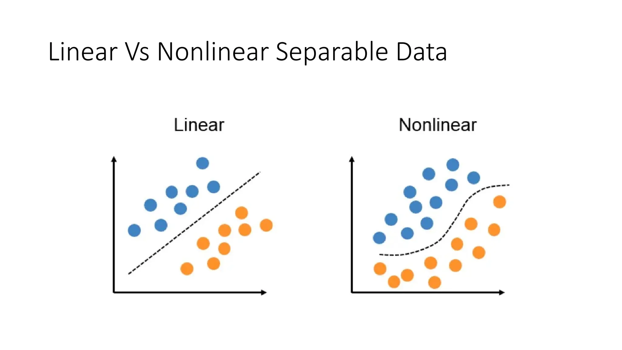
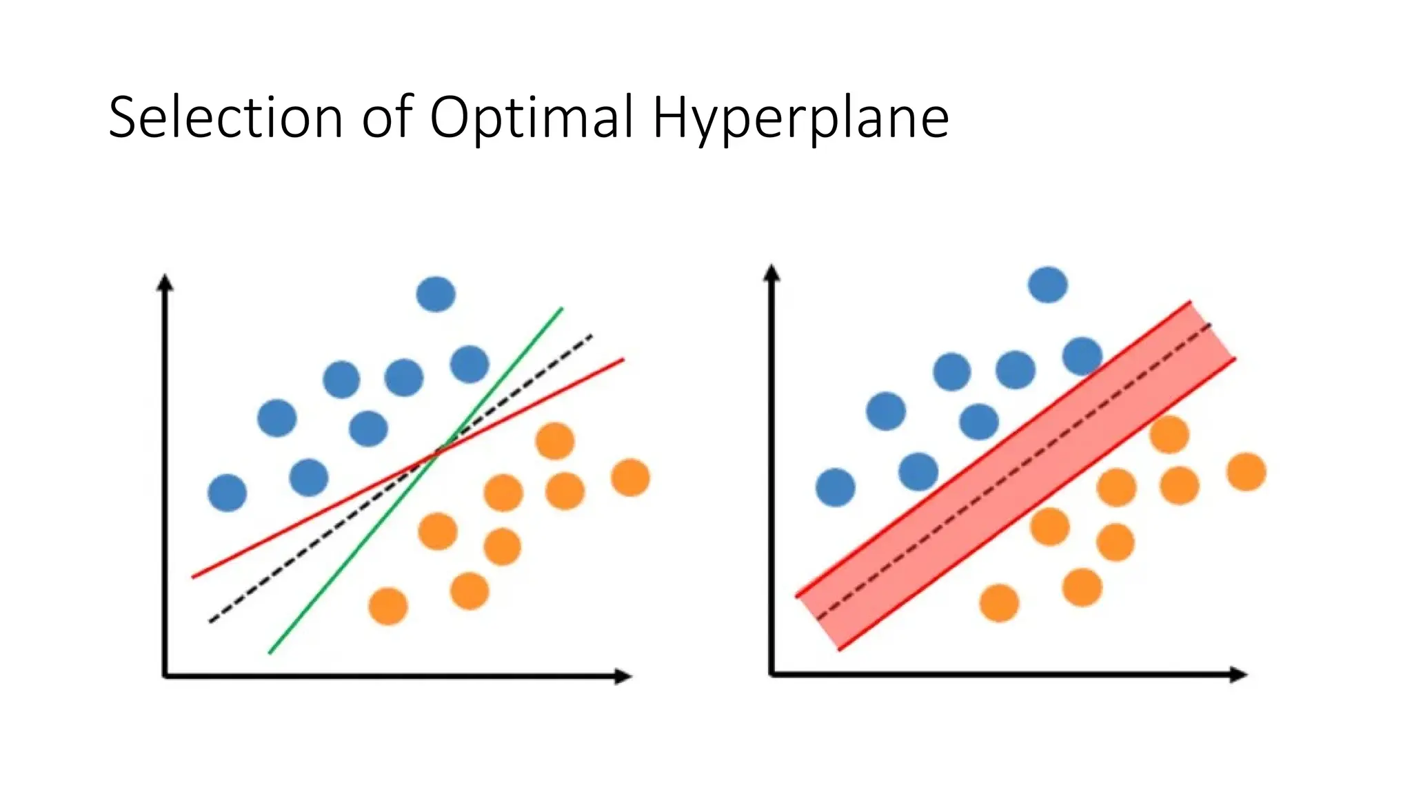
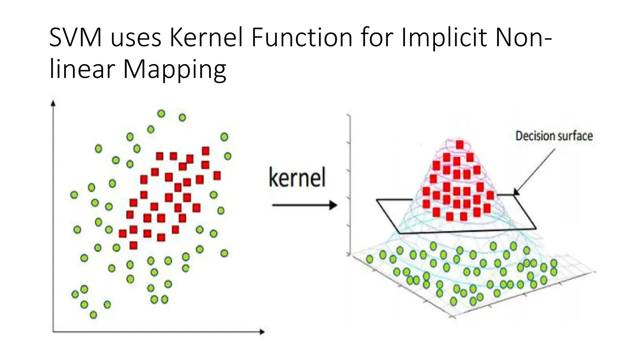
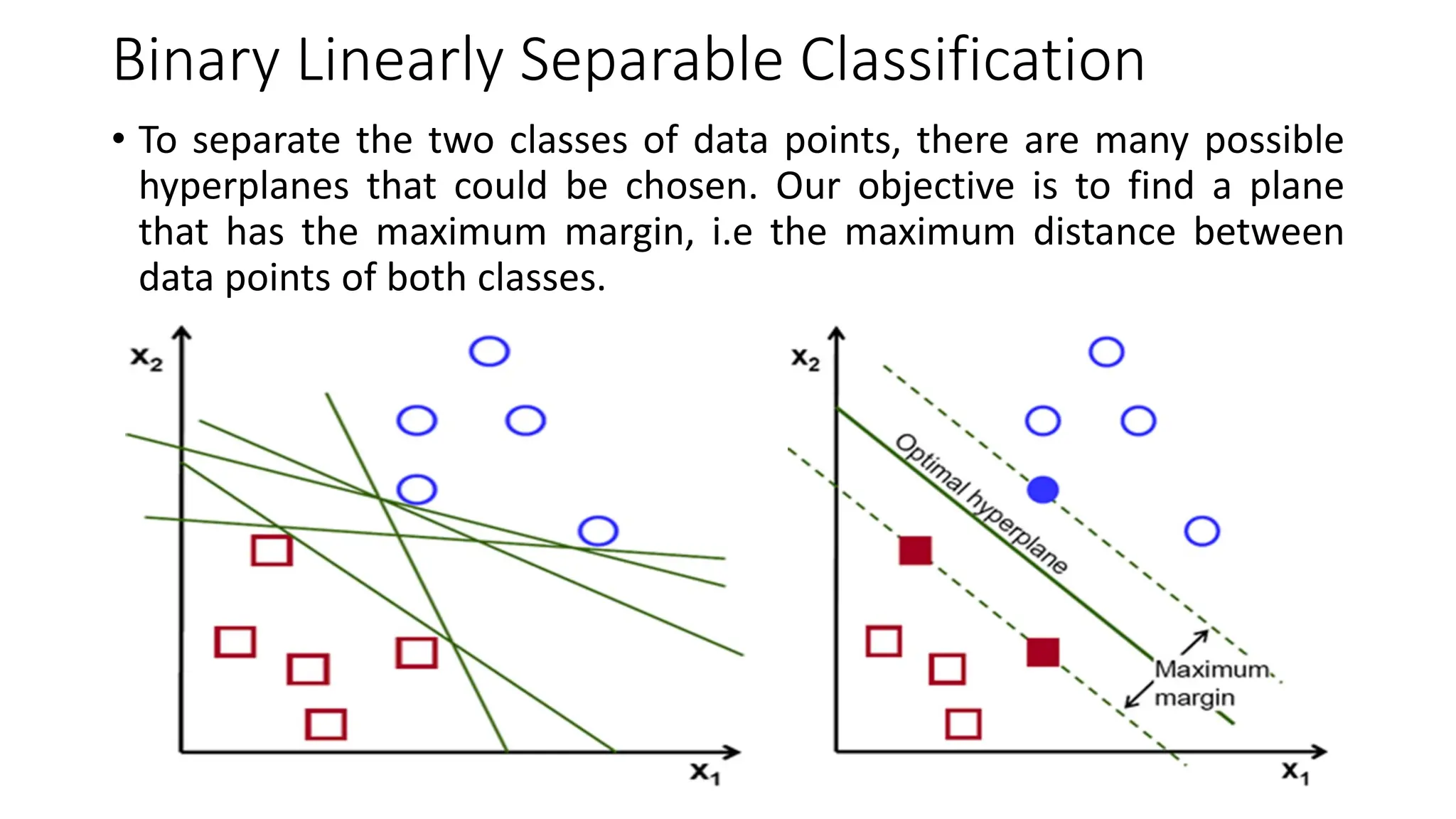
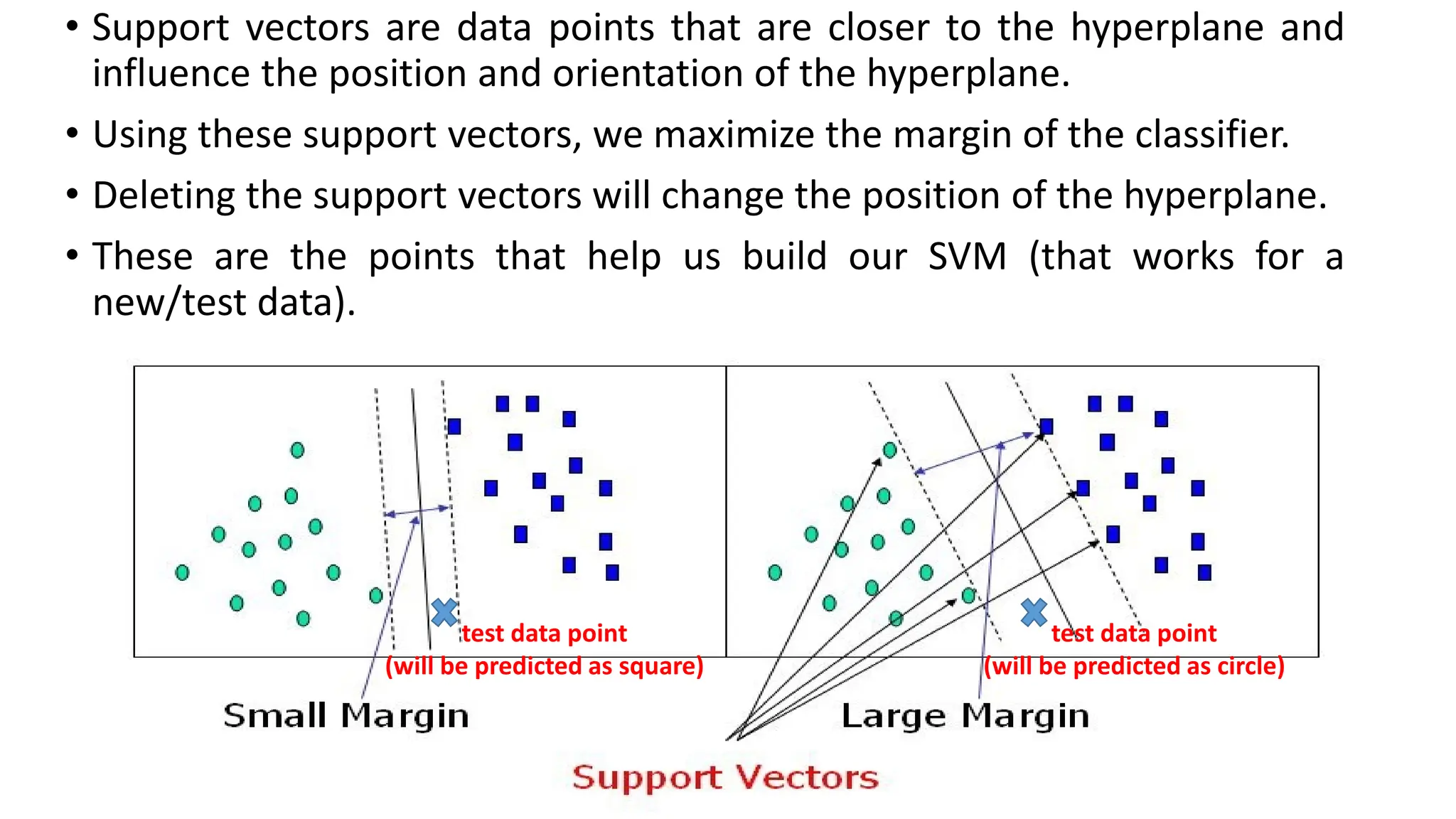
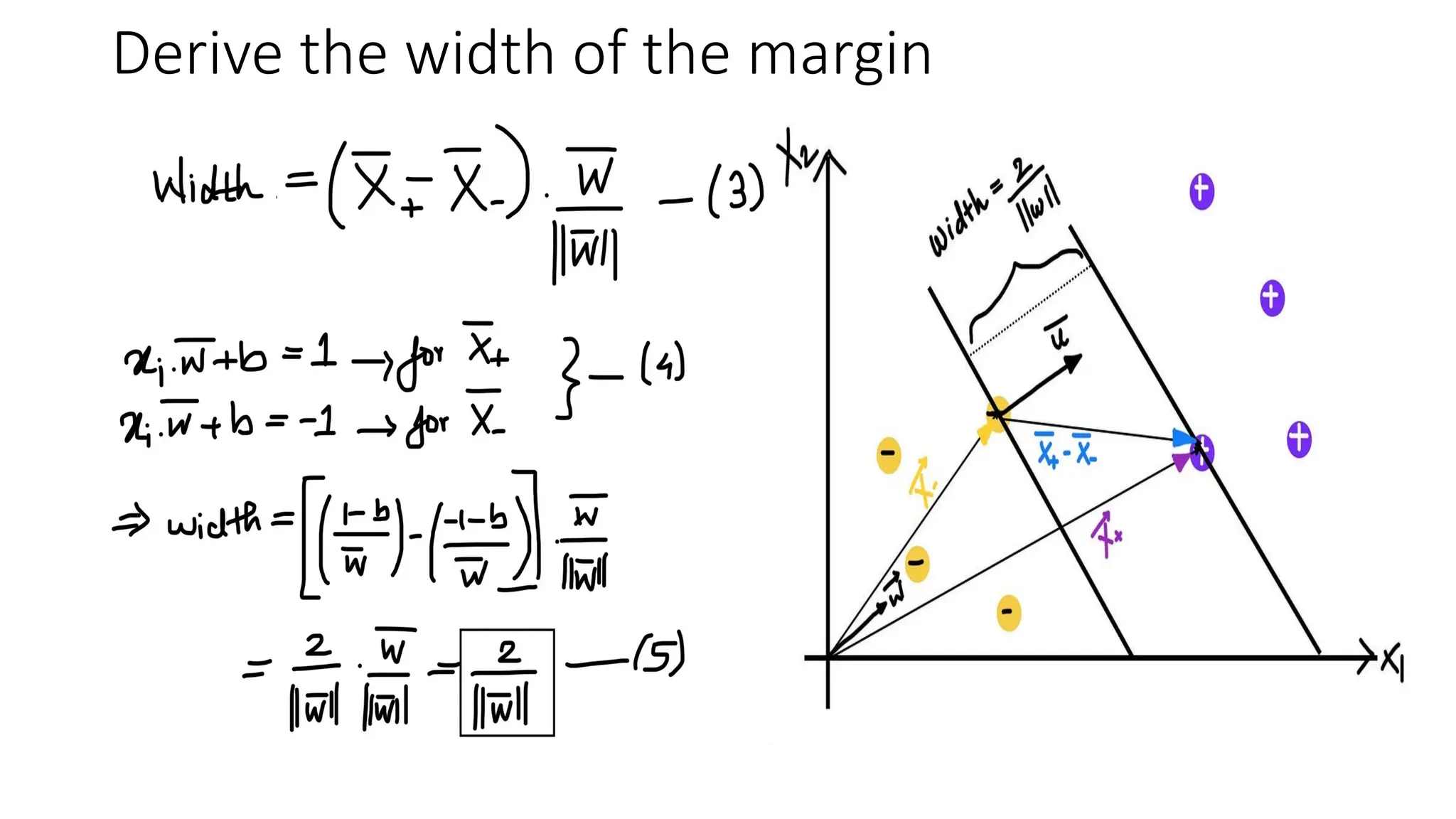
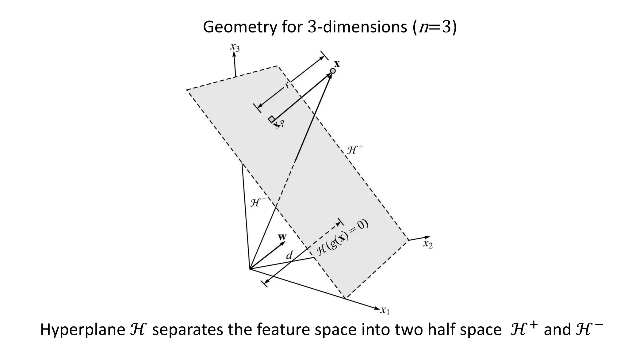
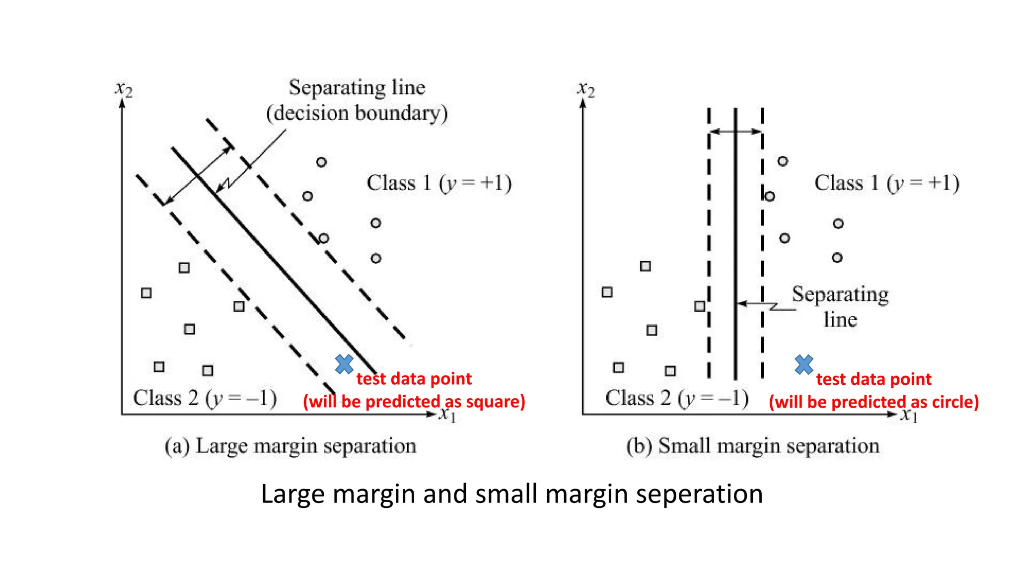
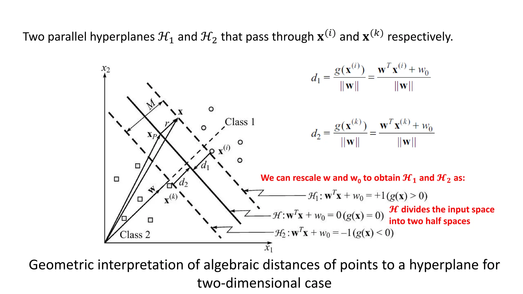
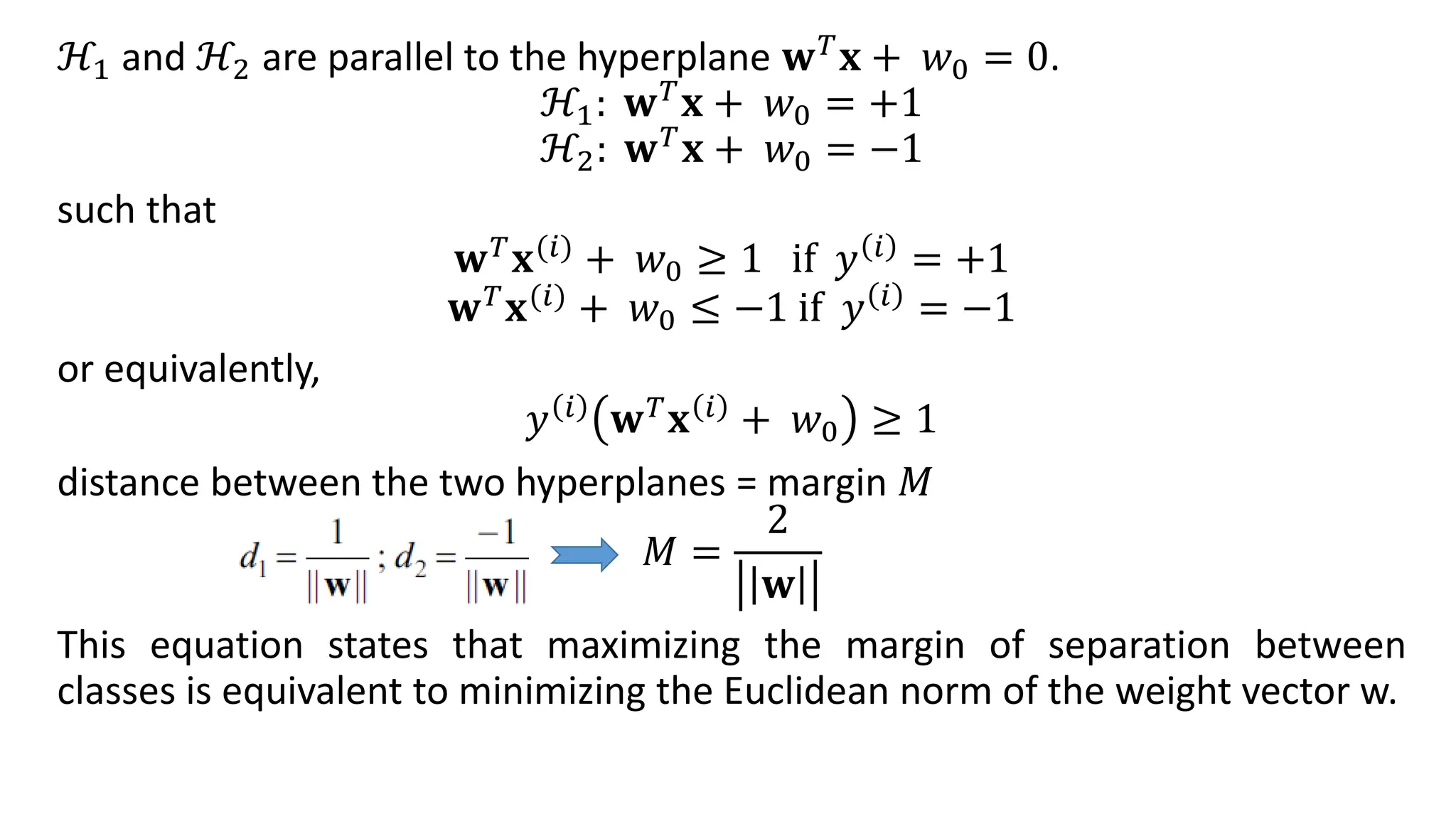
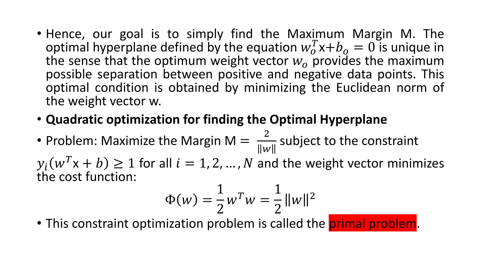
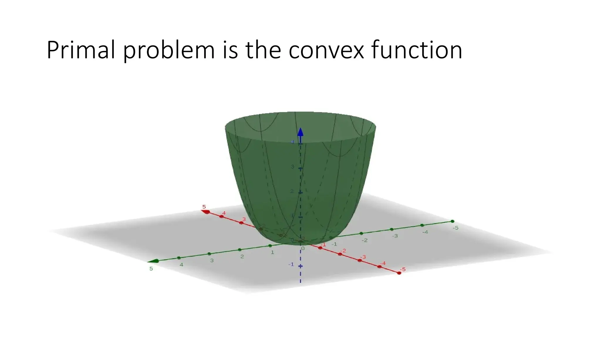
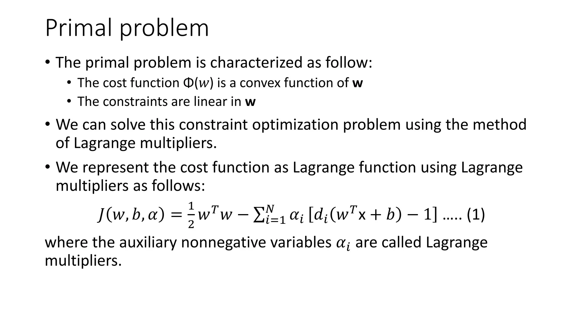
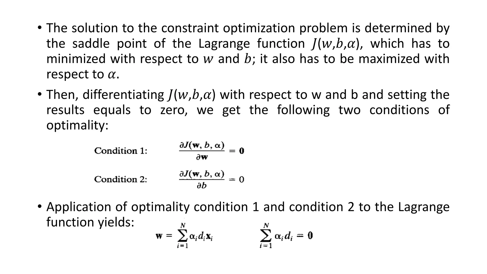
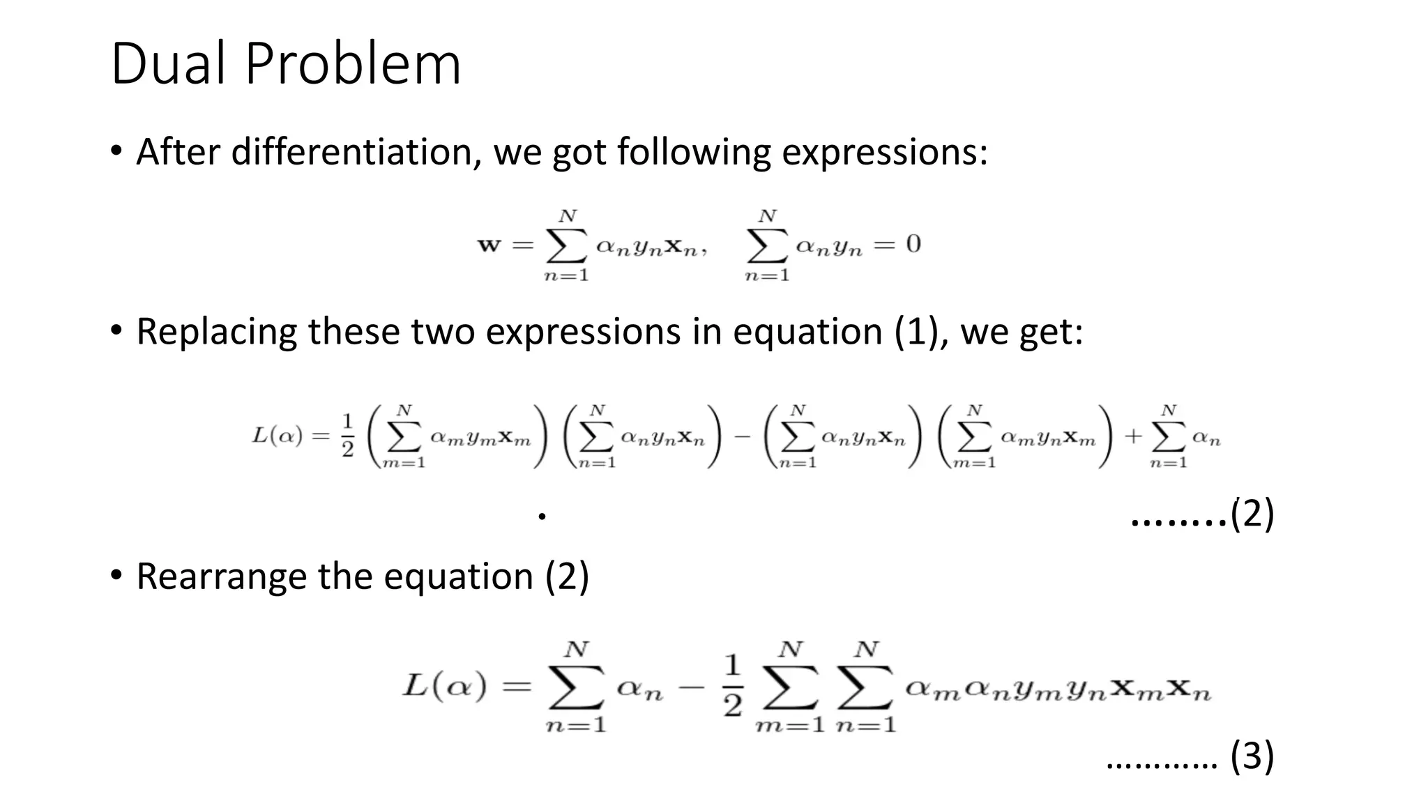
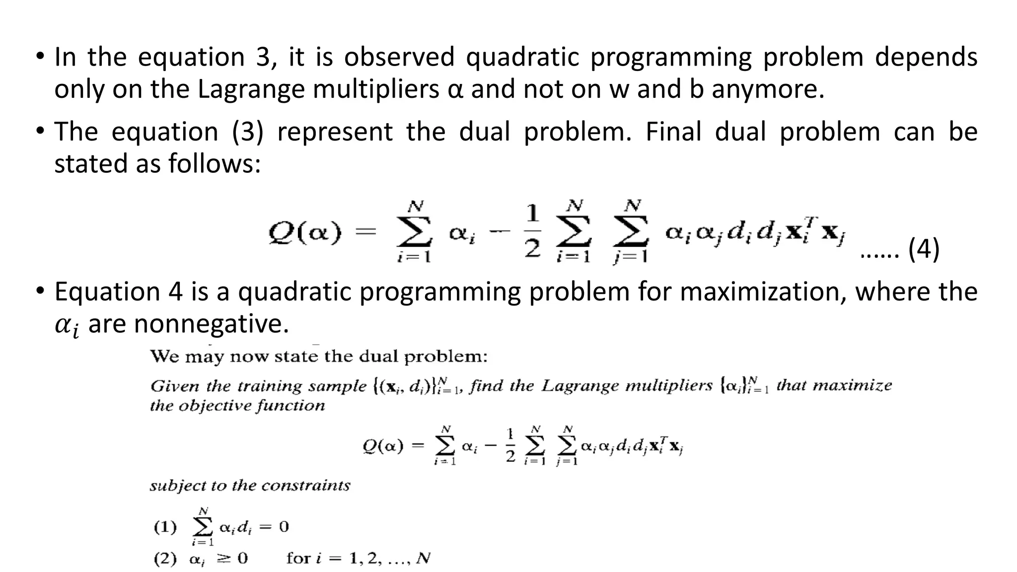
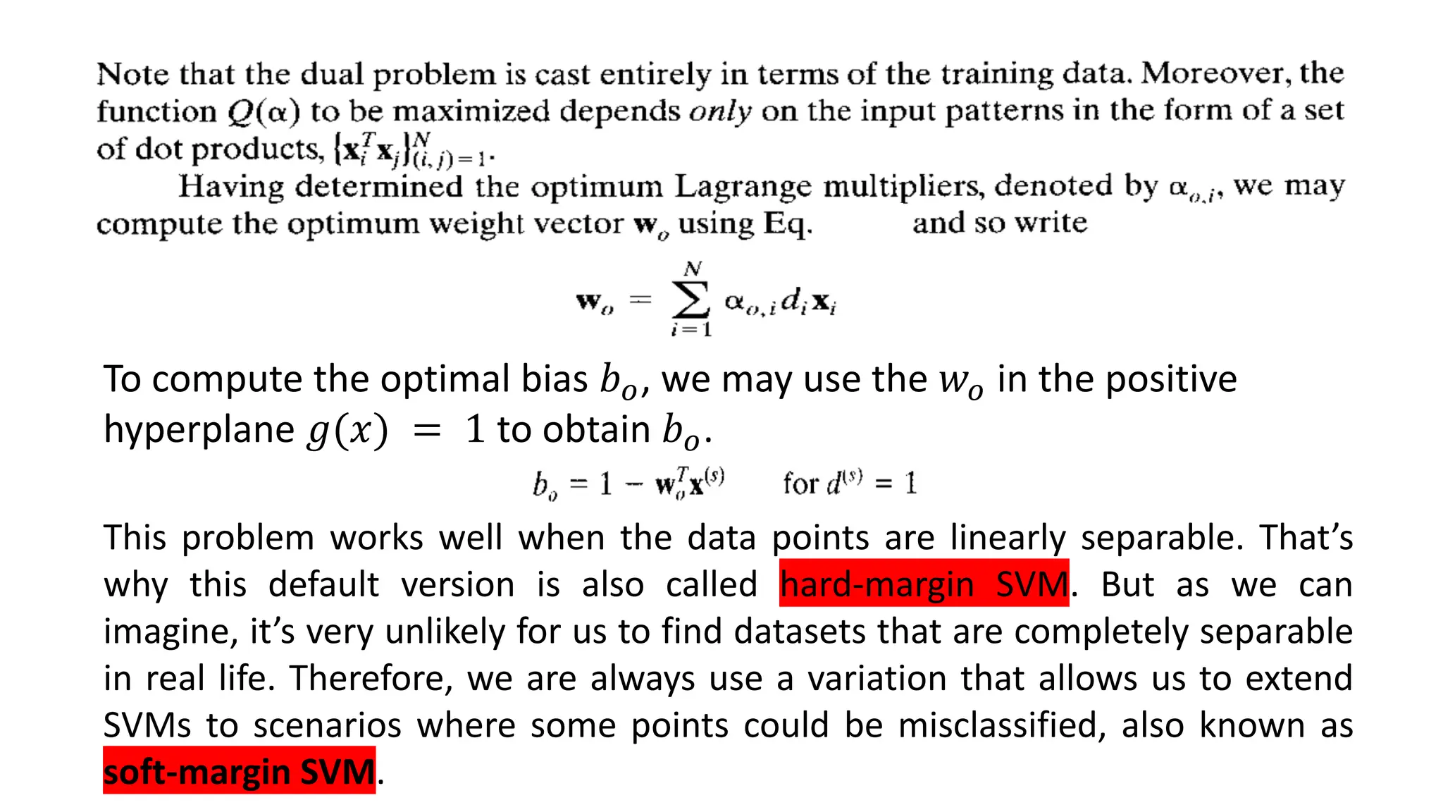
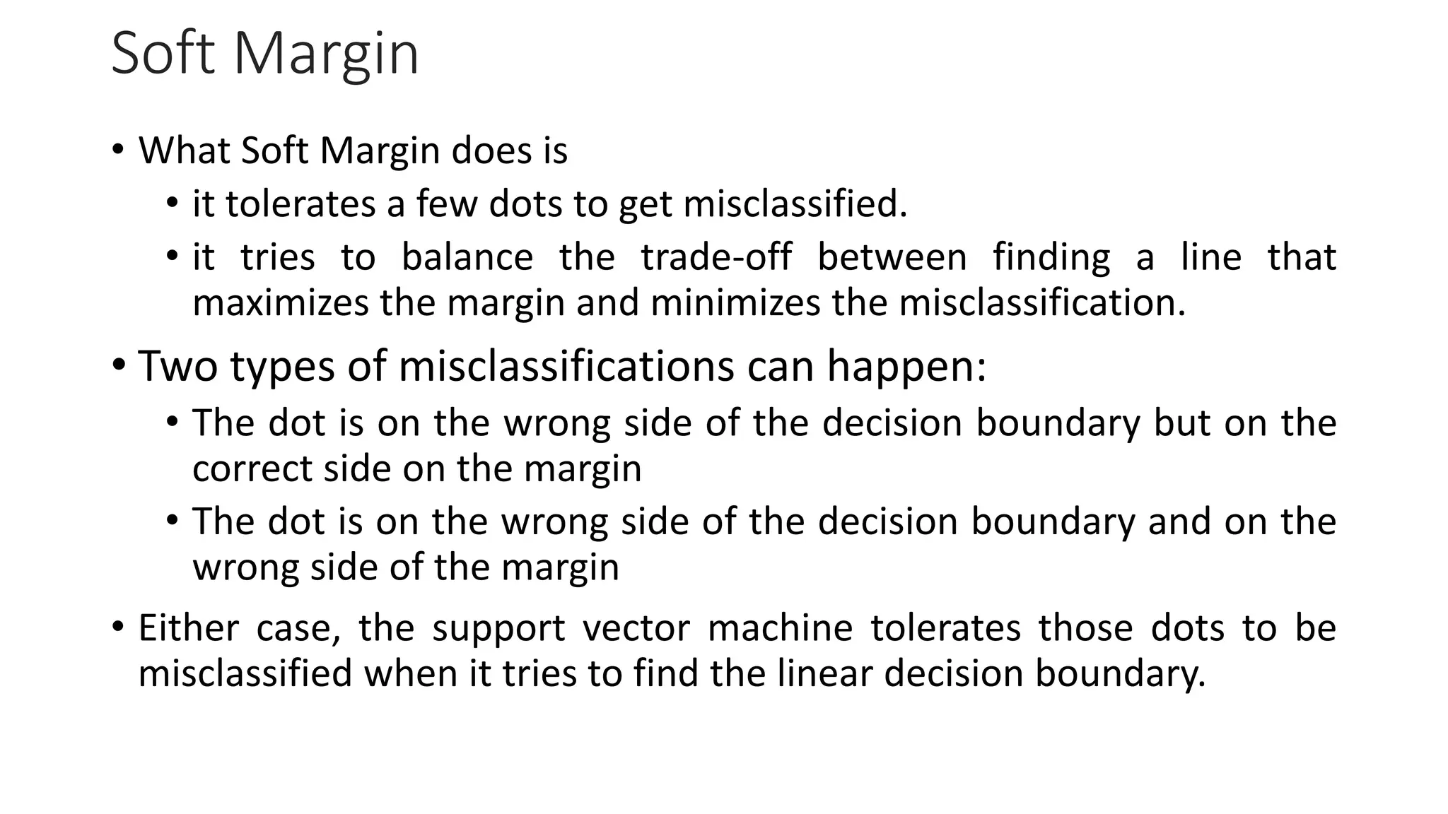
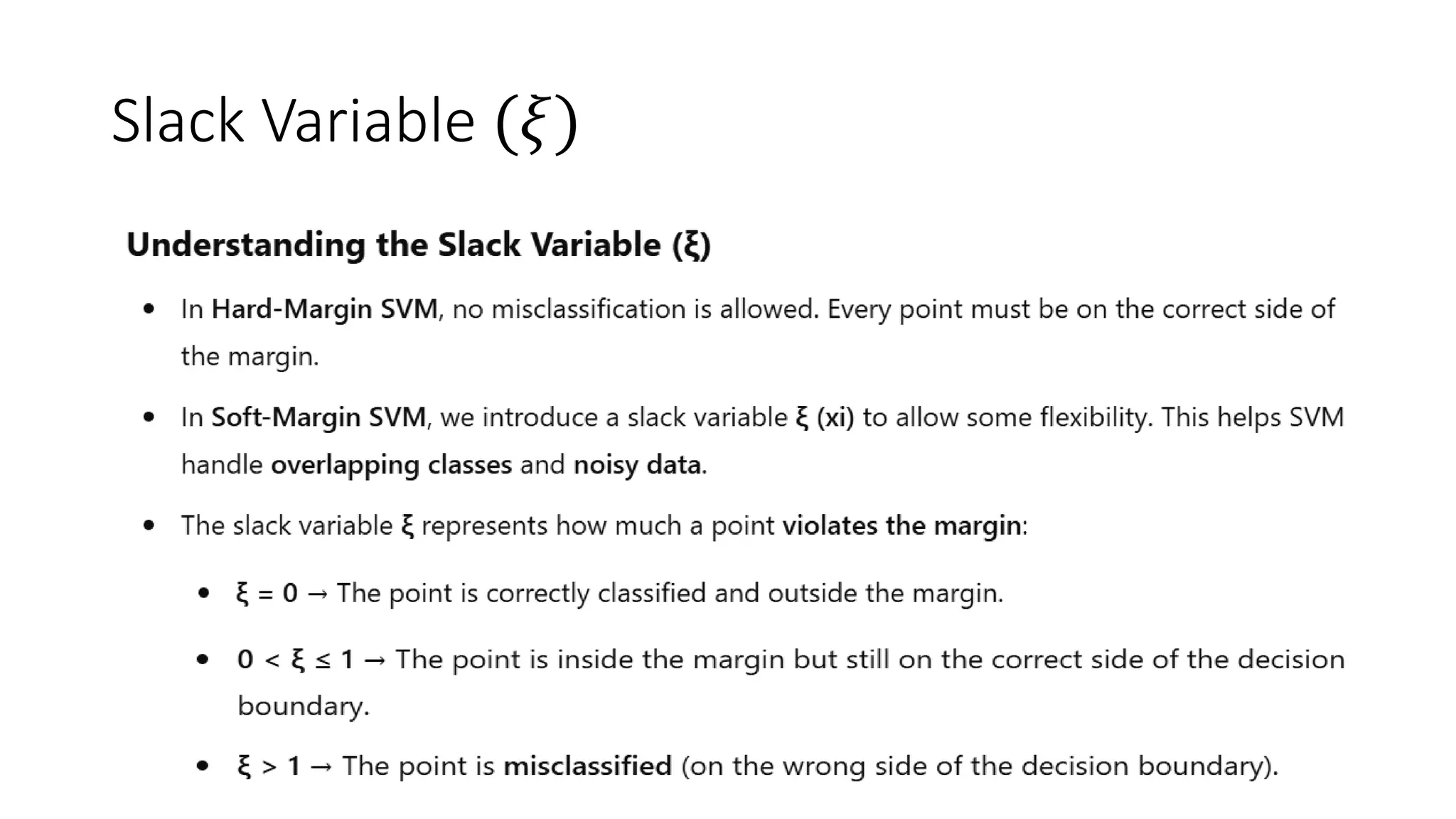
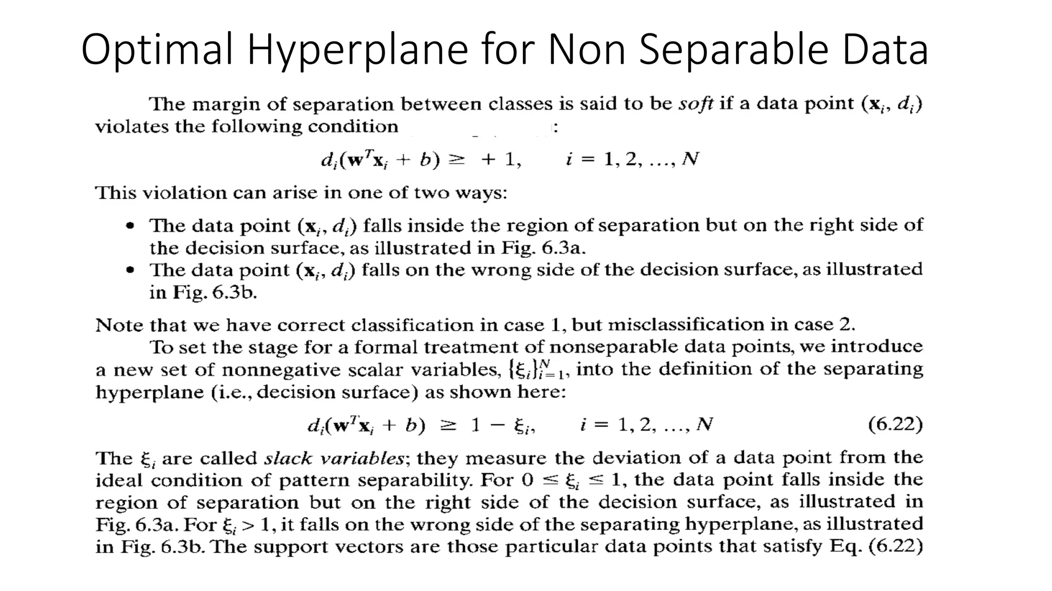
Support Vector Machine (SVM) is a supervised learning algorithm used for classification and regression by finding an optimal hyperplane that maximizes the margin between different classes. It identifies support vectors, which are the closest data points to the hyperplane, ensuring robustness to overfitting. When data is linearly separable, SVM finds a straight-line boundary, while for non-linear cases, it uses kernel functions (like polynomial, RBF, or sigmoid) to map data into a higher-dimensional space where it becomes separable. The optimization problem aims to minimize the norm of the weight vector while satisfying margin constraints. With advantages like effective handling of high-dimensional data and suitability for both small and large datasets, SVM is widely applied in text classification, image recognition, and bioinformatics.SVM operates by mapping input features into a high-dimensional space and constructing a decision boundary (hyperplane) that best separates different classes. The optimal hyperplane is chosen to maximize the margin, which is the distance between the closest data points (support vectors) from each class to the hyperplane.SVM’s performance largely depends on the choice of kernel functions, which transform input data into a higher-dimensional space where it becomes easier to classify. Commonly used kernels include the linear kernel for simple separable data, the polynomial kernel for capturing interactions between features, and the radial basis function (RBF) kernel for complex, non-linear patterns. The regularization parameter
𝐶
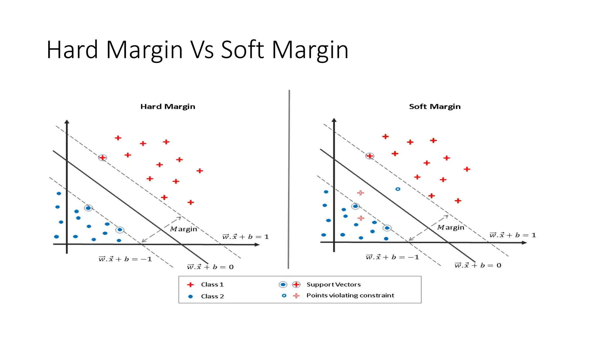
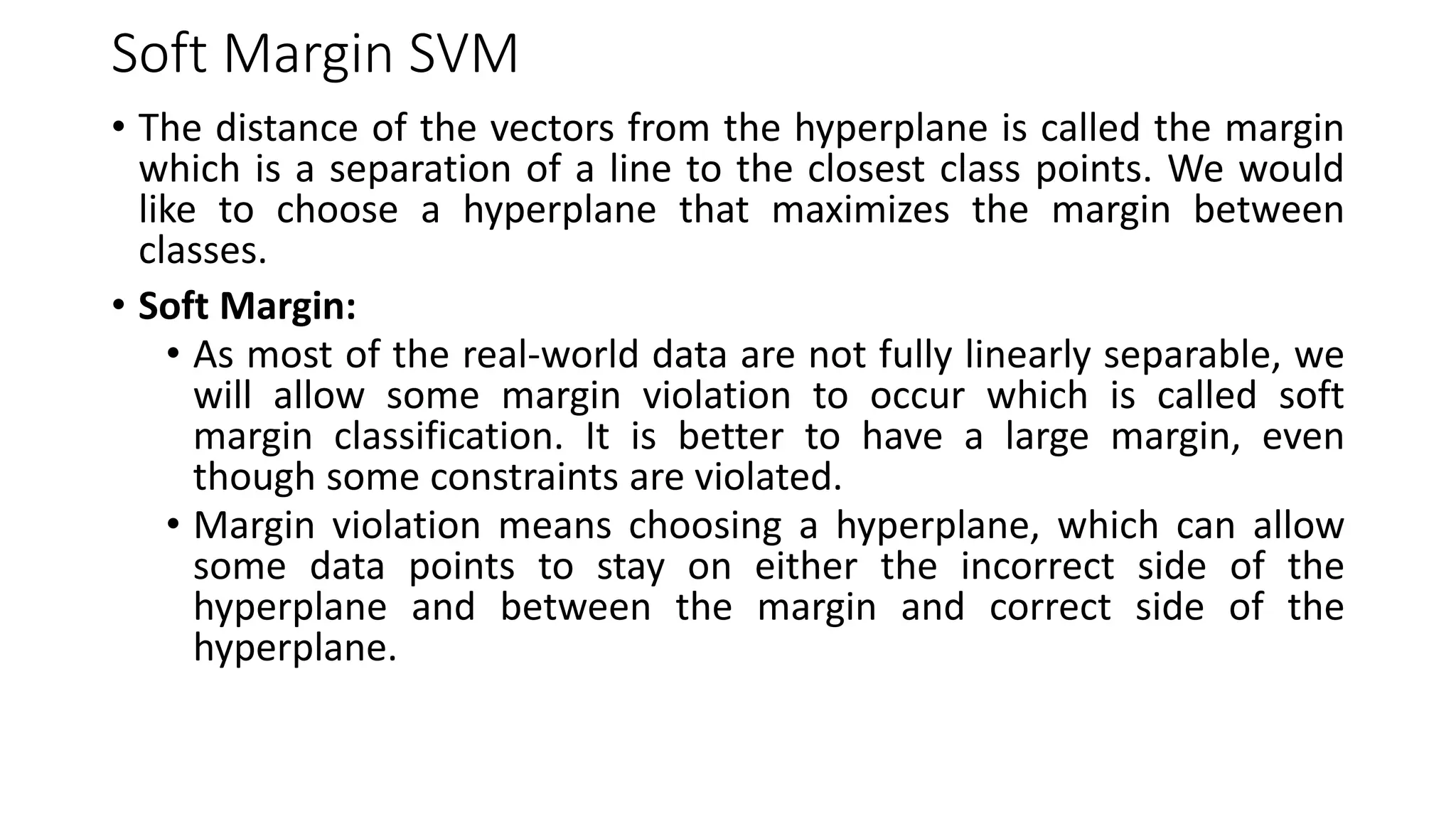
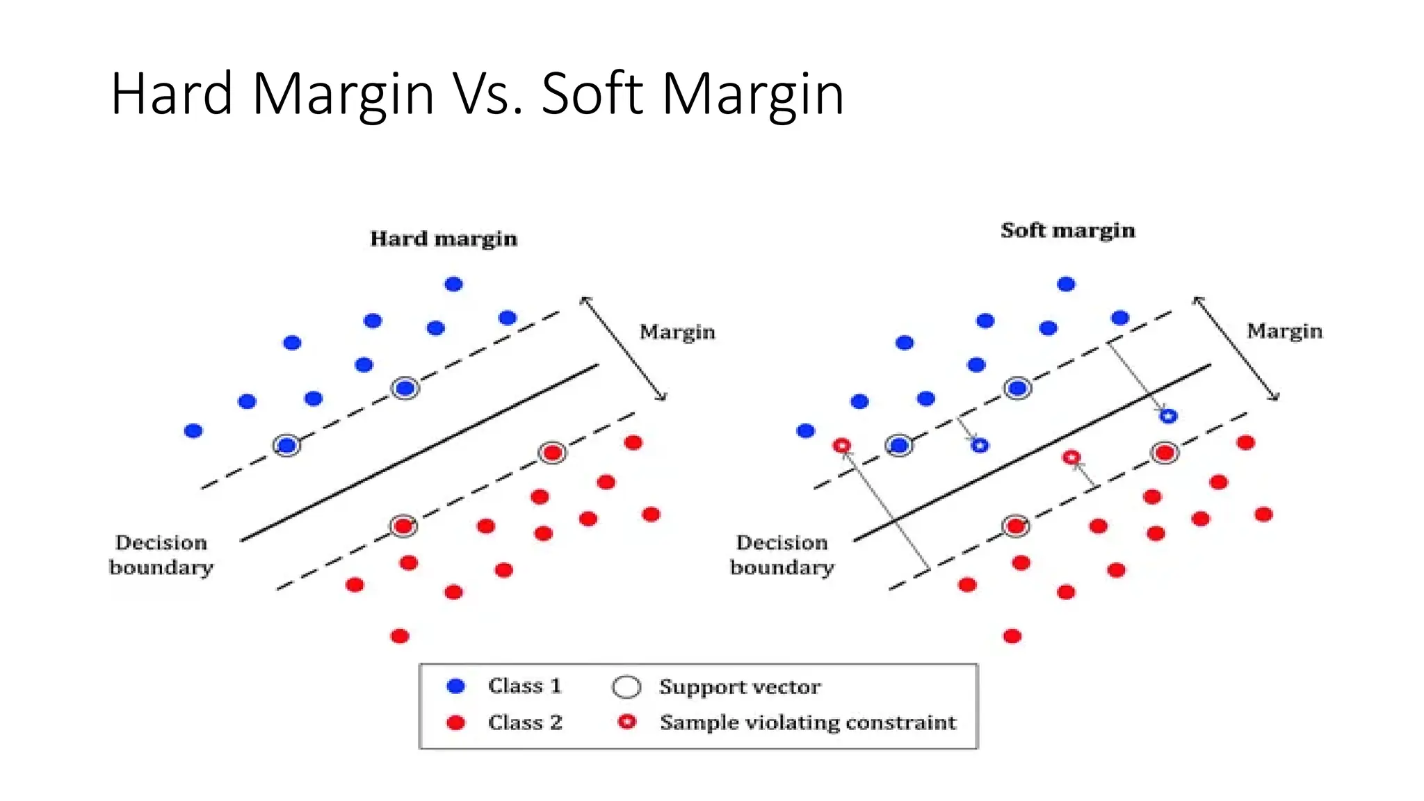
C controls the trade-off between maximizing the margin and minimizing classification errors, with higher values leading to lower bias but higher variance. Additionally, the soft margin approach allows some misclassification by introducing slack variables, making SVM more flexible in handling noisy data.
Despite its strengths, SVM has limitations, such as high computational cost for large datasets and difficulty in selecting the right kernel and hyperparameters. Training time increases significantly as the number of samples grows, especially for non-linear SVMs using complex kernels. Moreover, SVM does not provide direct probability estimates, requiring additional techniques like Platt scaling for probabilistic outputs. However, with proper tuning and kernel selection, SVM remains a powerful tool in various domains, including natural language processing, medical diagnosis, and financial fraud detection.


![SVM[Support vector Machine] Machine learning](https://cdn.slidesharecdn.com/ss_thumbnails/svm-250403184638-1cd9afdb-thumbnail.jpg?width=640&height=640&fit=bounds)


![[ML]-SVM2.ppt.pdf](https://cdn.slidesharecdn.com/ss_thumbnails/ml-svm2-230916145832-2580c8e3-thumbnail.jpg?width=640&height=640&fit=bounds)


