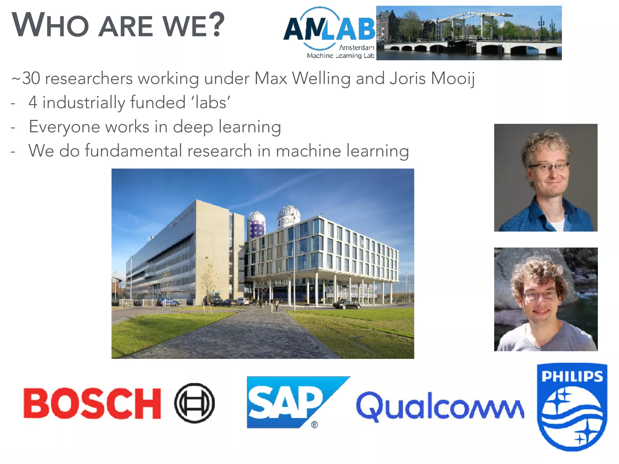
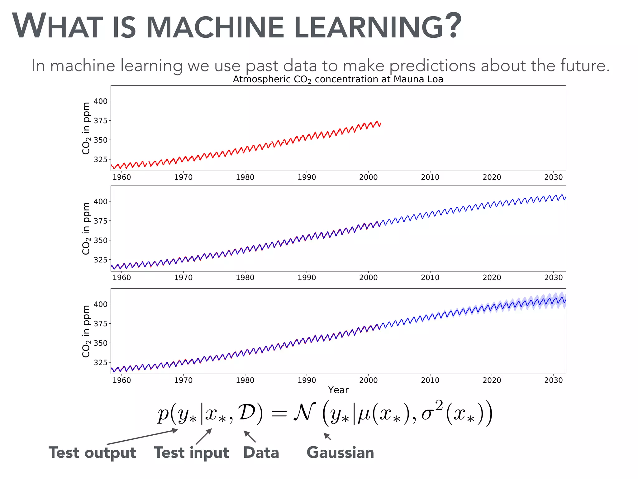
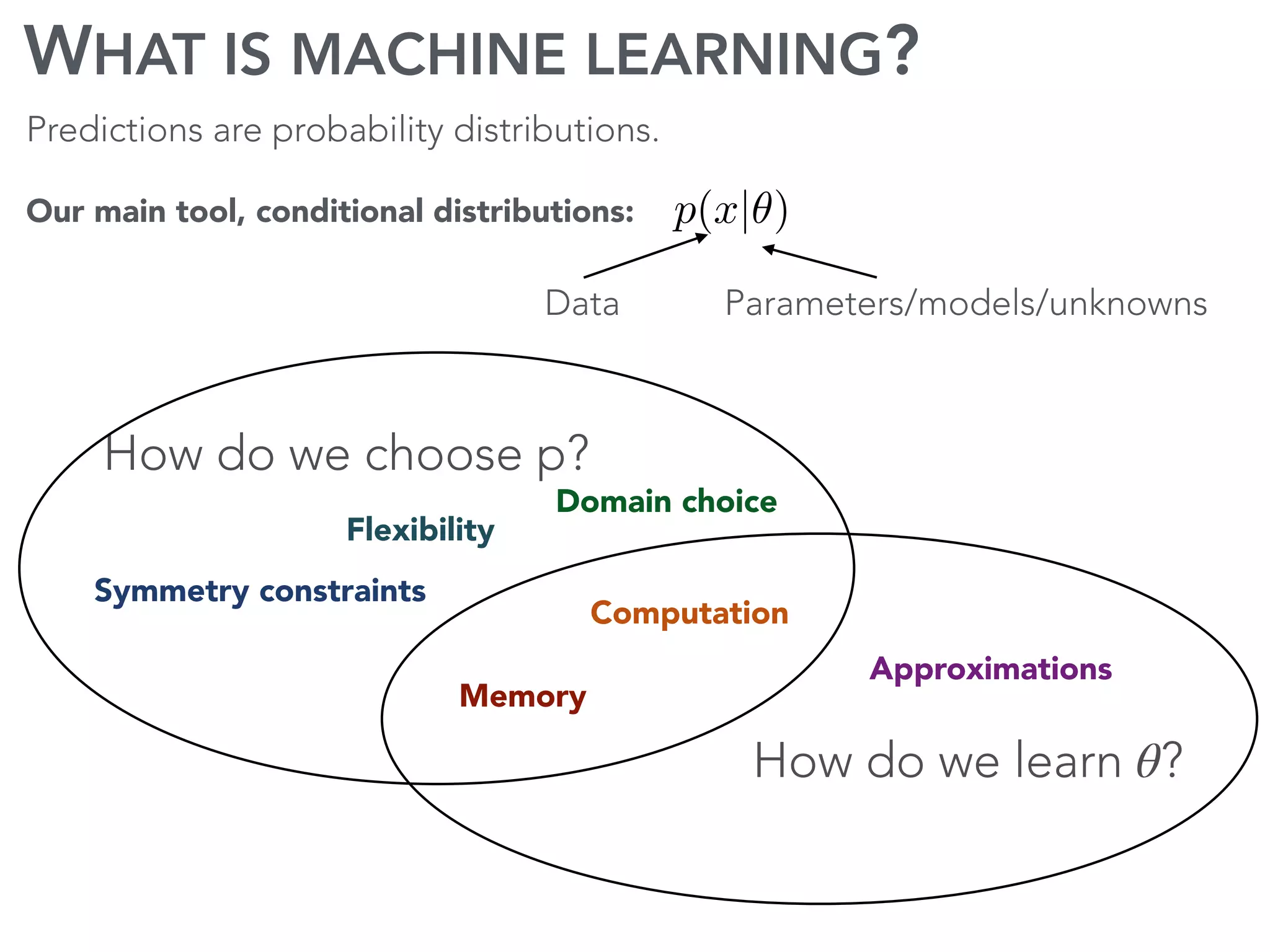
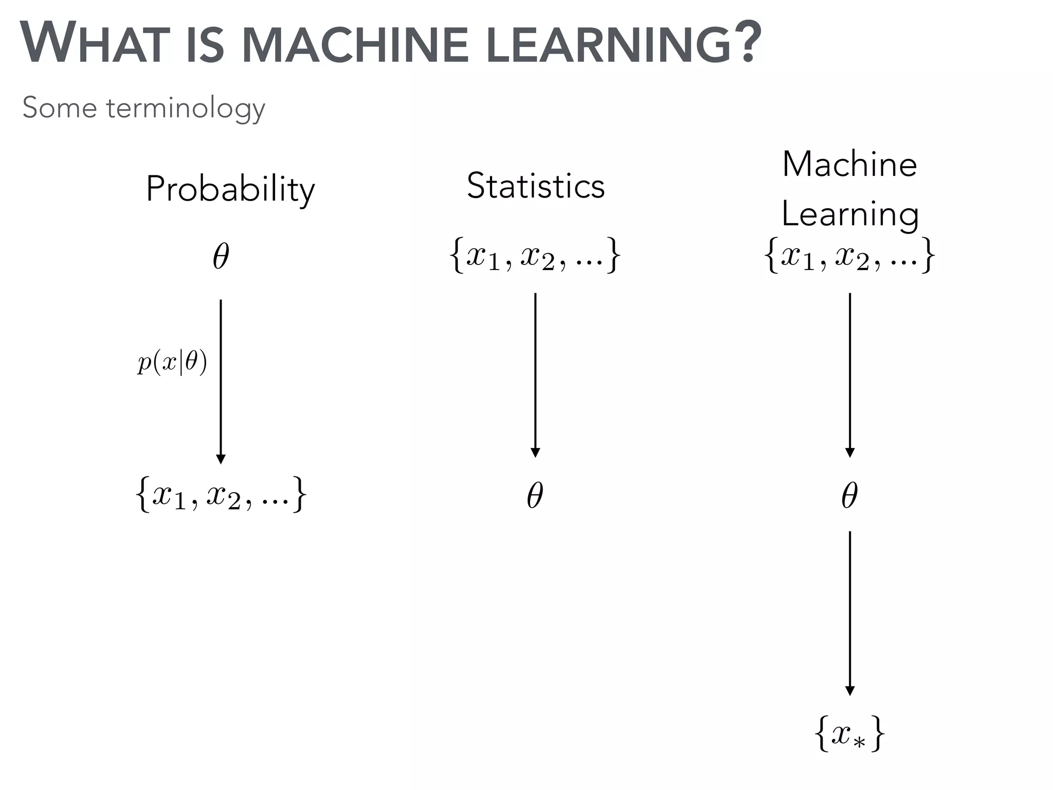
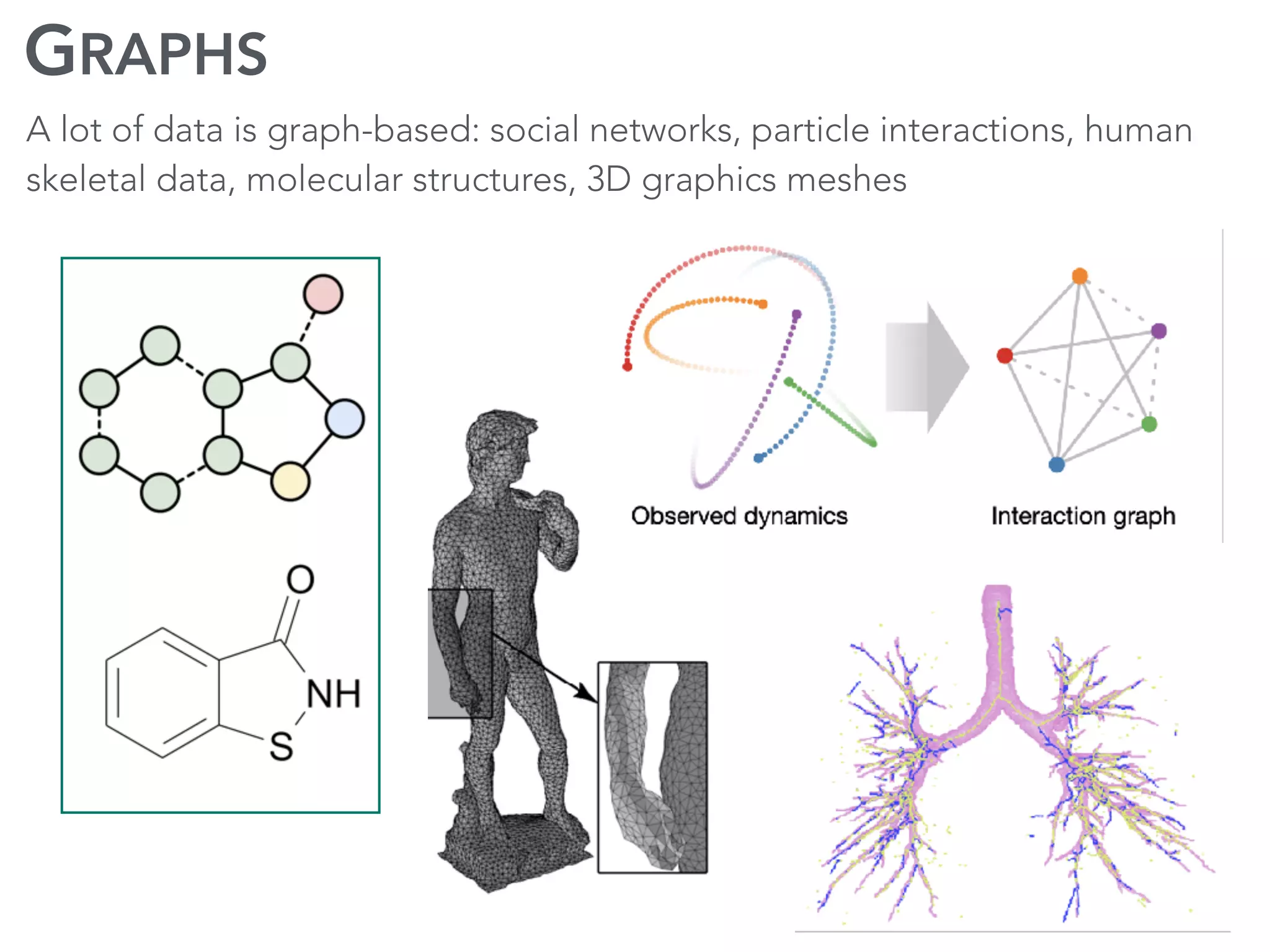
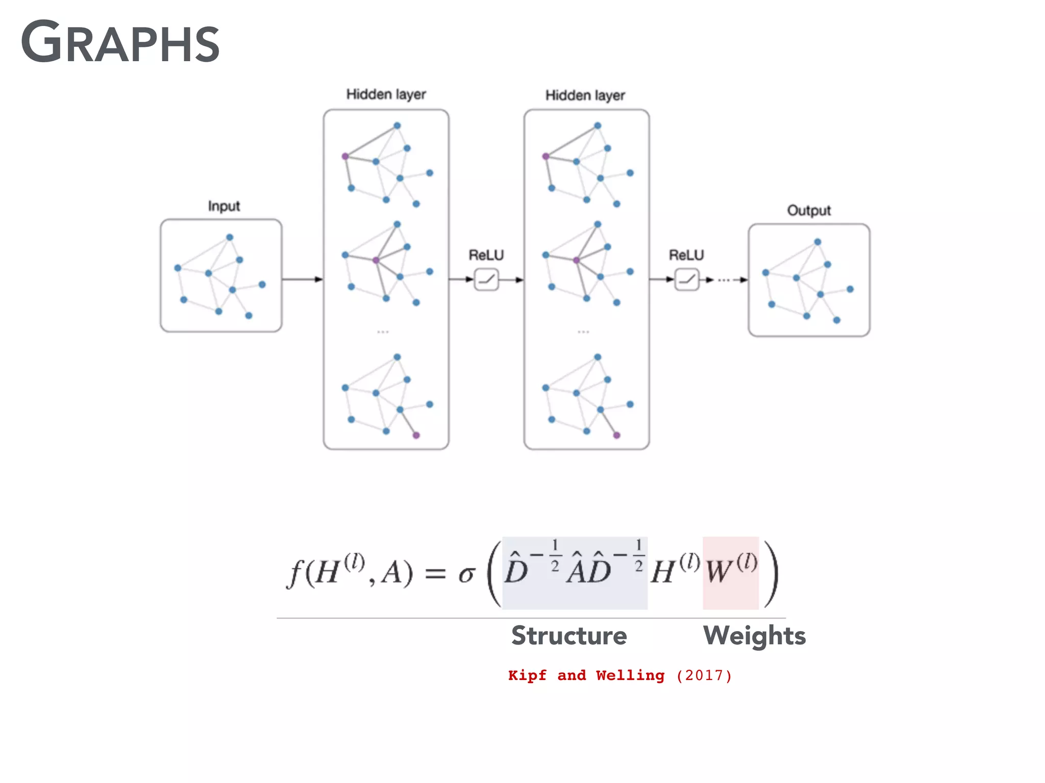
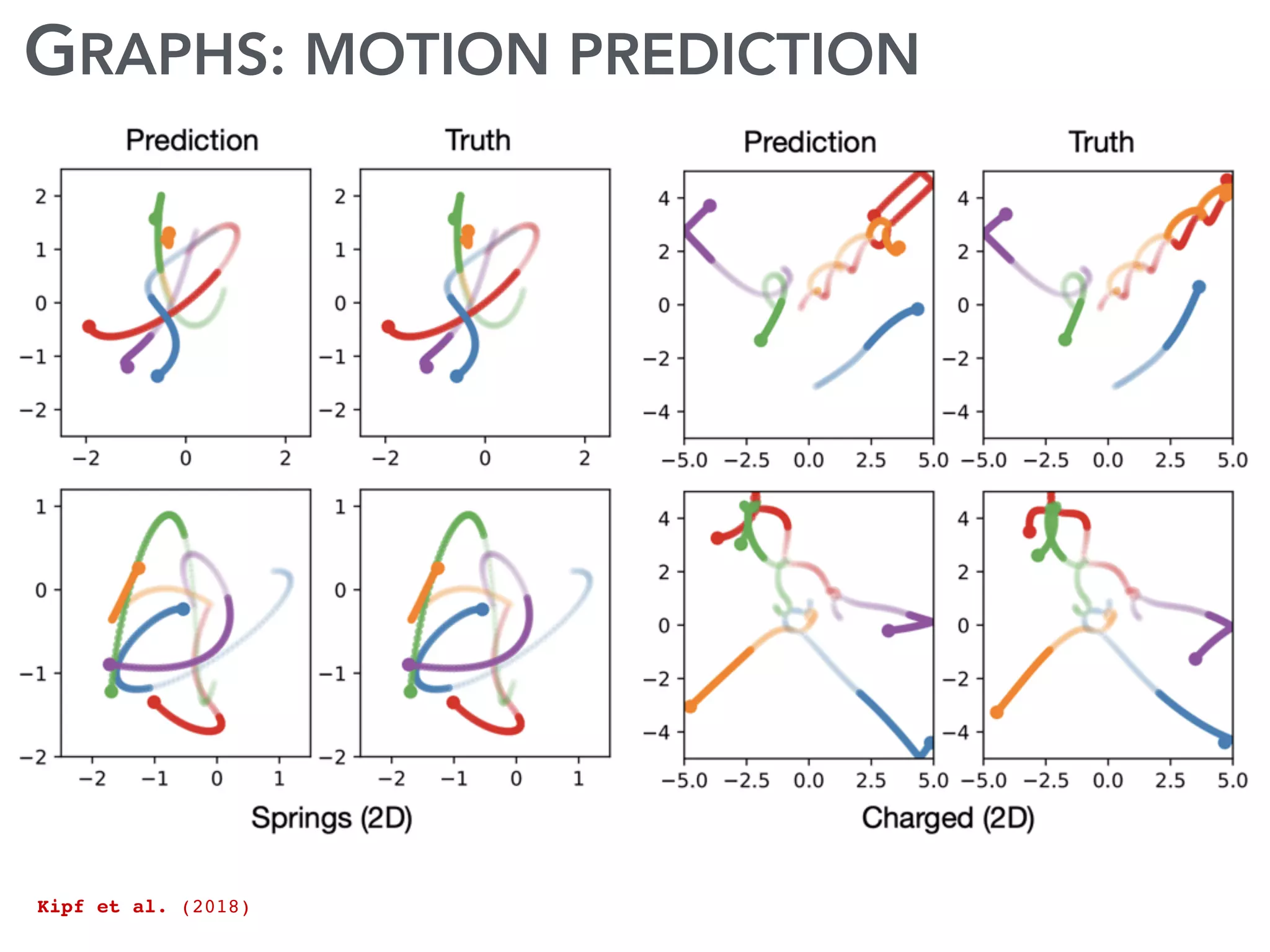
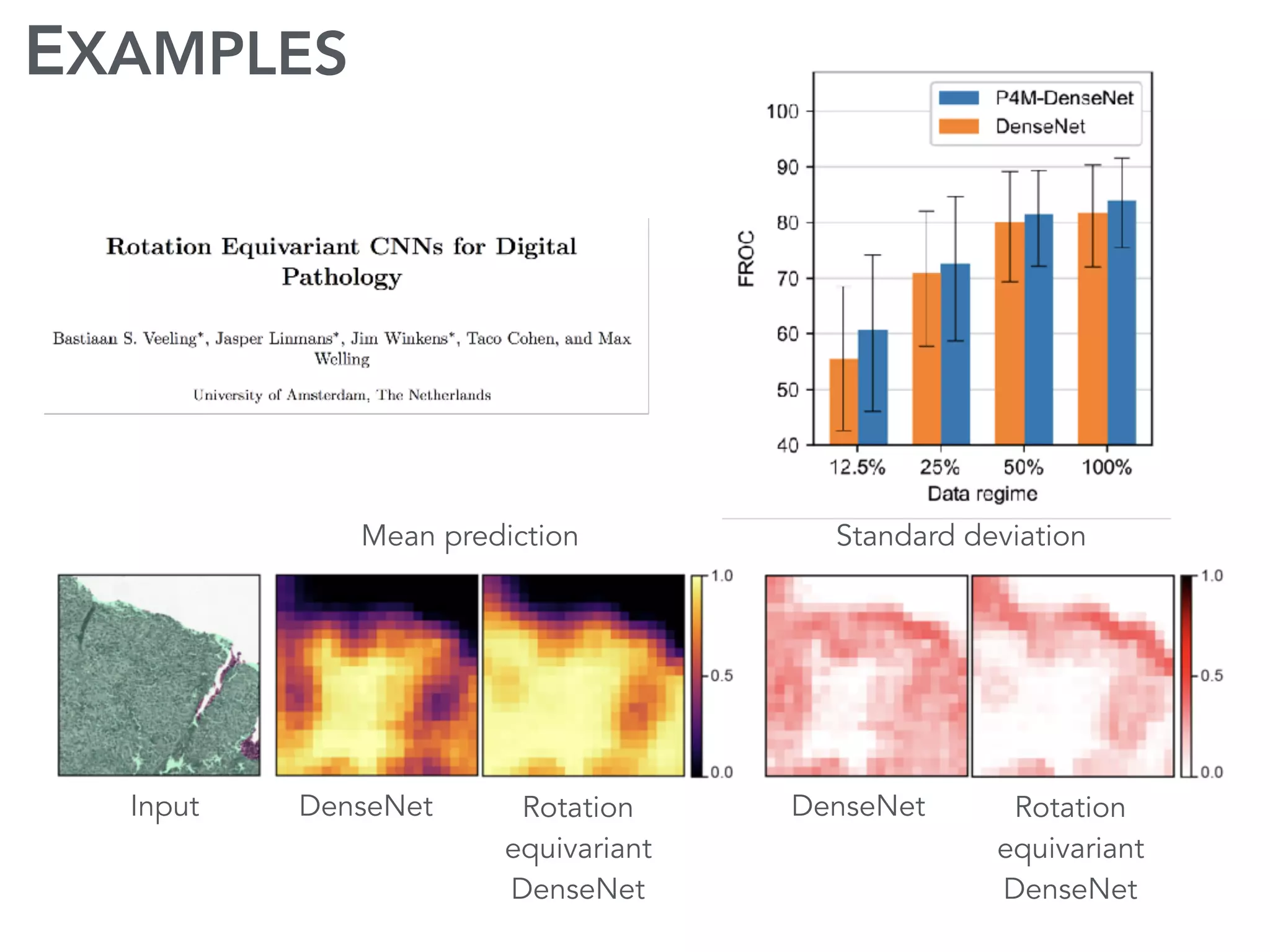
The document discusses current research and advances in machine learning conducted by a team of researchers focused on deep learning. It covers key concepts such as variational methods, normalizing flows, and symmetry in graphs, as well as their applications in various fields like medical imaging and generative modeling. The research emphasizes probability distributions and the use of past data to make predictions about the future.
![VARIATIONAL METHODS
Approximate inference
Intractable
p(✓|D) =
p(D|✓)p(✓)
p(D)
=
p(D|✓)p(✓)
R
p(D|✓)p(✓) d✓
Log-likelihood Regulariser
ELBO
q (✓) = arg min DKL [q (✓)kp(✓|D)]
= arg min
Z
q (✓) log
q (✓)
p(✓|D)
d✓
= arg min
Z
q (✓) log
q (✓)p(D)
p(D|✓)p(✓)
d✓
= arg max Eq (✓)[p(D|✓)] + DKL [q (✓)kp(✓)]
q (✓) = arg min DKL [q (✓)kp(✓|D)]
= arg min
Z
q (✓) log
q (✓)
p(✓|D)
d✓
= arg min
Z
q (✓) log
q (✓)p(D)
p(D|✓)p(✓)
d✓
= arg max Eq (✓)[p(D|✓)] + DKL [q (✓)kp(✓)]
q (✓) = arg min DKL [q (✓)kp(✓|D)]
= arg min
Z
q (✓) log
q (✓)
p(✓|D)
d✓
= arg min
Z
q (✓) log
q (✓)p(D)
p(D|✓)p(✓)
d✓
= arg max Eq (✓)[p(D|✓)] + DKL [q (✓)kp(✓)]
‘Distance’ between
distributions
q (✓) = arg min DKL [q (✓)kp(✓|D)]
= arg min
Z
q (✓) log
q (✓)
p(✓|D)
d✓
= arg min
Z
q (✓) log
q (✓)p(D)
p(D|✓)p(✓)
d✓
= arg max Eq (✓)[p(D|✓)] DKL [q (✓)kp(✓)]
p(✓|D) =
p(D|✓)p(✓)
p(D)
=
p(D|✓)p(✓)
R
p(D|✓)p(✓) d✓](https://image.slidesharecdn.com/worrall-190320142822/75/Machine-Learning-Today-Current-Research-And-Advances-From-AMLAB-UvA-8-2048.jpg)
![VARIATIONAL METHODS
Approximate inference
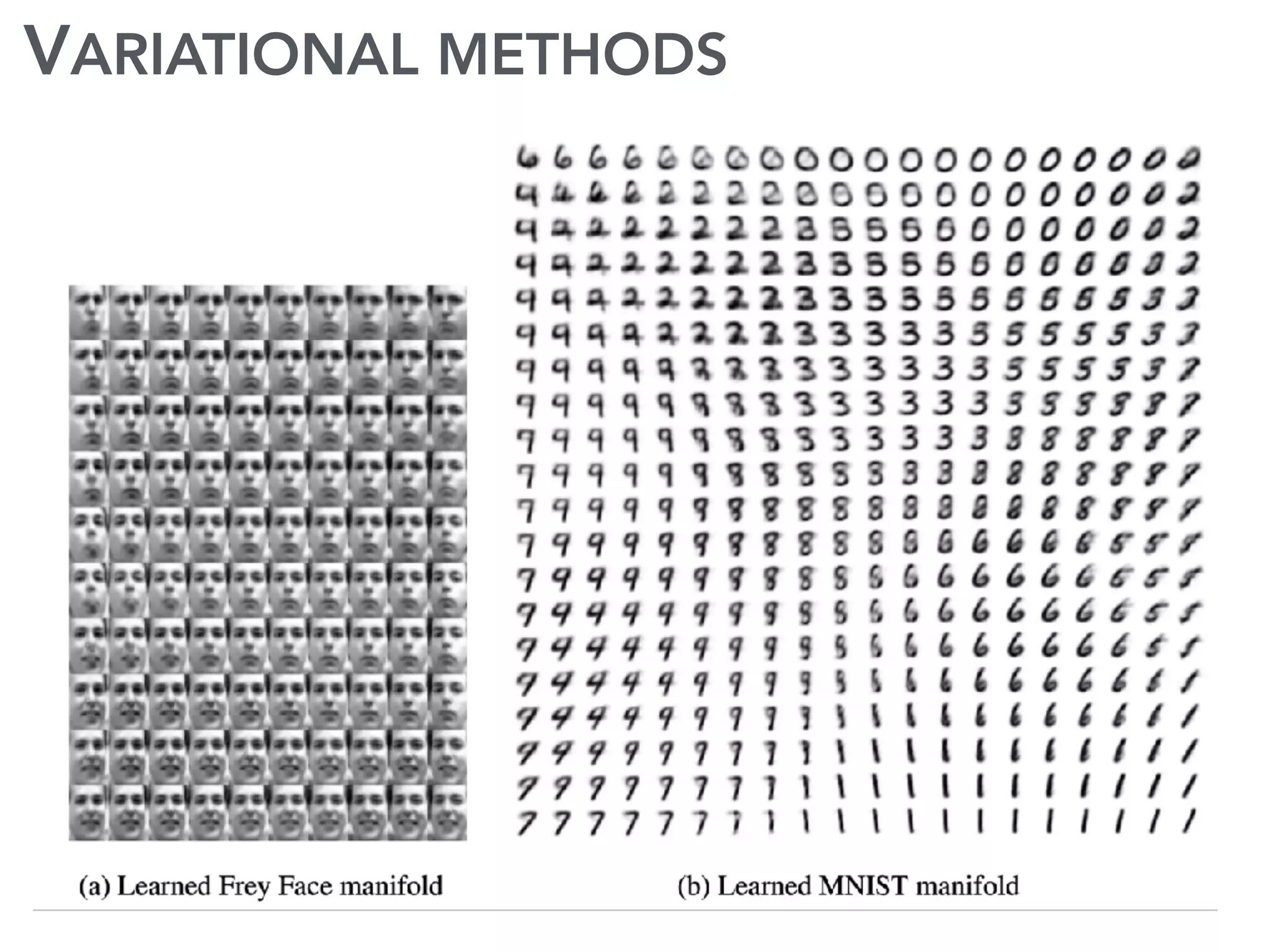
If we use latents (each x has a z) then we have a variational auto-encoder
arg max Ep(x)
⇥
Eq (z|x)[p(x|z)] DKL [q (z|x)kp(z)]
⇤
= arg min q (✓) log
q (✓)
p(✓|D)
d✓
= arg min
Z
q (✓) log
q (✓)p(D)
p(D|✓)p(✓)
d✓
= arg max Eq (✓)[p(D|✓)] DKL [q (✓)kp(✓)]
Neural network
Kingma and Welling (2013)](https://image.slidesharecdn.com/worrall-190320142822/75/Machine-Learning-Today-Current-Research-And-Advances-From-AMLAB-UvA-9-2048.jpg)
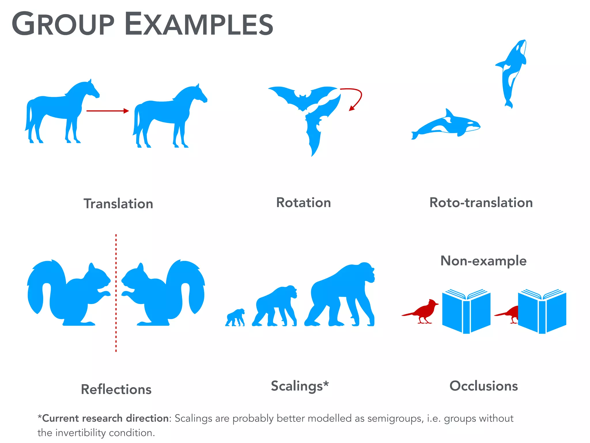
![SYMMETRY?
f(I) = f(T✓[I])
Notational aside:
T✓[I](x) = I(x ✓)
T✓[I](x) = I(R 1
✓ x)
T [I] = (I µ)/. 1
function/
feature mapping
image
transformation
Symmetry is a property of functions/tasks, e.g.
Classification
Disentangling
(cocktail party)
Signal discovery/detection
e.g. Geometric translation
e.g. Geometric rotation
e.g. Pixel normalisation
Set of input transformations leaving invariantS✓[f](I) = f(T✓[I])](https://image.slidesharecdn.com/worrall-190320142822/75/Machine-Learning-Today-Current-Research-And-Advances-From-AMLAB-UvA-17-2048.jpg)
 = f(T✓[I])S✓[f](I) = f(T✓[I])S✓[f](I) = f(T✓[I])S✓[f](I) = f(T✓[I])
transformation in feature space
Mapping preserves algebraic
structure of transformation
Different representations of same
transformation
https://github.com/vdumoulin/conv_arithmetic
Convolution (and correlation)
[I ⇤ W](x ✓) = T✓[I] ⇤ W(x)
S✓ = Id
Invariance
Convolutions Symmetry](https://image.slidesharecdn.com/worrall-190320142822/75/Machine-Learning-Today-Current-Research-And-Advances-From-AMLAB-UvA-18-2048.jpg)
 =
X
x2Z2
I(x)W(R 1
✓ x)
[I ⇤ W](y) =
X
x2Z2
I(x)W(x y)
[I ⇤ W](✓, y) =
X
x2Z2
I(x)W(R 1
✓ x y)
[I ⇤ W](✓) =
X
x2Z2
I(x)T✓[W](x)Group convolution
[I ⇤ W](✓) =
X
x2Z2
T✓[I](x)W(x)Semigroup convolution](https://image.slidesharecdn.com/worrall-190320142822/75/Machine-Learning-Today-Current-Research-And-Advances-From-AMLAB-UvA-20-2048.jpg)


![VARIATIONAL METHODS
Approximate inference
Intractable
p(✓|D) =
p(D|✓)p(✓)
p(D)
=
p(D|✓)p(✓)
R
p(D|✓)p(✓) d✓
Log-likelihood Regulariser
ELBO
q (✓) = arg min DKL [q (✓)kp(✓|D)]
= arg min
Z
q (✓) log
q (✓)
p(✓|D)
d✓
= arg min
Z
q (✓) log
q (✓)p(D)
p(D|✓)p(✓)
d✓
= arg max Eq (✓)[p(D|✓)] + DKL [q (✓)kp(✓)]
q (✓) = arg min DKL [q (✓)kp(✓|D)]
= arg min
Z
q (✓) log
q (✓)
p(✓|D)
d✓
= arg min
Z
q (✓) log
q (✓)p(D)
p(D|✓)p(✓)
d✓
= arg max Eq (✓)[p(D|✓)] + DKL [q (✓)kp(✓)]
q (✓) = arg min DKL [q (✓)kp(✓|D)]
= arg min
Z
q (✓) log
q (✓)
p(✓|D)
d✓
= arg min
Z
q (✓) log
q (✓)p(D)
p(D|✓)p(✓)
d✓
= arg max Eq (✓)[p(D|✓)] + DKL [q (✓)kp(✓)]
‘Distance’ between
distributions
q (✓) = arg min DKL [q (✓)kp(✓|D)]
= arg min
Z
q (✓) log
q (✓)
p(✓|D)
d✓
= arg min
Z
q (✓) log
q (✓)p(D)
p(D|✓)p(✓)
d✓
= arg max Eq (✓)[p(D|✓)] DKL [q (✓)kp(✓)]
p(✓|D) =
p(D|✓)p(✓)
p(D)
=
p(D|✓)p(✓)
R
p(D|✓)p(✓) d✓](https://crownmelresort.com/image.slidesharecdn.com/worrall-190320142822/75/Machine-Learning-Today-Current-Research-And-Advances-From-AMLAB-UvA-8-2048.jpg)
![VARIATIONAL METHODS
Approximate inference
If we use latents (each x has a z) then we have a variational auto-encoder
arg max Ep(x)
⇥
Eq (z|x)[p(x|z)] DKL [q (z|x)kp(z)]
⇤
= arg min q (✓) log
q (✓)
p(✓|D)
d✓
= arg min
Z
q (✓) log
q (✓)p(D)
p(D|✓)p(✓)
d✓
= arg max Eq (✓)[p(D|✓)] DKL [q (✓)kp(✓)]
Neural network
Kingma and Welling (2013)](https://crownmelresort.com/image.slidesharecdn.com/worrall-190320142822/75/Machine-Learning-Today-Current-Research-And-Advances-From-AMLAB-UvA-9-2048.jpg)


![SYMMETRY?
f(I) = f(T✓[I])
Notational aside:
T✓[I](x) = I(x ✓)
T✓[I](x) = I(R 1
✓ x)
T [I] = (I µ)/. 1
function/
feature mapping
image
transformation
Symmetry is a property of functions/tasks, e.g.
Classification
Disentangling
(cocktail party)
Signal discovery/detection
e.g. Geometric translation
e.g. Geometric rotation
e.g. Pixel normalisation
Set of input transformations leaving invariantS✓[f](I) = f(T✓[I])](https://crownmelresort.com/image.slidesharecdn.com/worrall-190320142822/75/Machine-Learning-Today-Current-Research-And-Advances-From-AMLAB-UvA-17-2048.jpg)
 = f(T✓[I])S✓[f](I) = f(T✓[I])S✓[f](I) = f(T✓[I])S✓[f](I) = f(T✓[I])
transformation in feature space
Mapping preserves algebraic
structure of transformation
Different representations of same
transformation
https://github.com/vdumoulin/conv_arithmetic
Convolution (and correlation)
[I ⇤ W](x ✓) = T✓[I] ⇤ W(x)
S✓ = Id
Invariance
Convolutions Symmetry](https://crownmelresort.com/image.slidesharecdn.com/worrall-190320142822/75/Machine-Learning-Today-Current-Research-And-Advances-From-AMLAB-UvA-18-2048.jpg)

 =
X
x2Z2
I(x)W(R 1
✓ x)
[I ⇤ W](y) =
X
x2Z2
I(x)W(x y)
[I ⇤ W](✓, y) =
X
x2Z2
I(x)W(R 1
✓ x y)
[I ⇤ W](✓) =
X
x2Z2
I(x)T✓[W](x)Group convolution
[I ⇤ W](✓) =
X
x2Z2
T✓[I](x)W(x)Semigroup convolution](https://crownmelresort.com/image.slidesharecdn.com/worrall-190320142822/75/Machine-Learning-Today-Current-Research-And-Advances-From-AMLAB-UvA-20-2048.jpg)


![[DL輪読会]Recent Advances in Autoencoder-Based Representation Learning](https://cdn.slidesharecdn.com/ss_thumbnails/20190119dljournalclubweb-190401063633-thumbnail.jpg?width=640&height=640&fit=bounds)

![[DL輪読会] off-policyなメタ強化学習](https://cdn.slidesharecdn.com/ss_thumbnails/20190405journalclub-190415082841-thumbnail.jpg?width=640&height=640&fit=bounds)