Download as ODP, PPTX
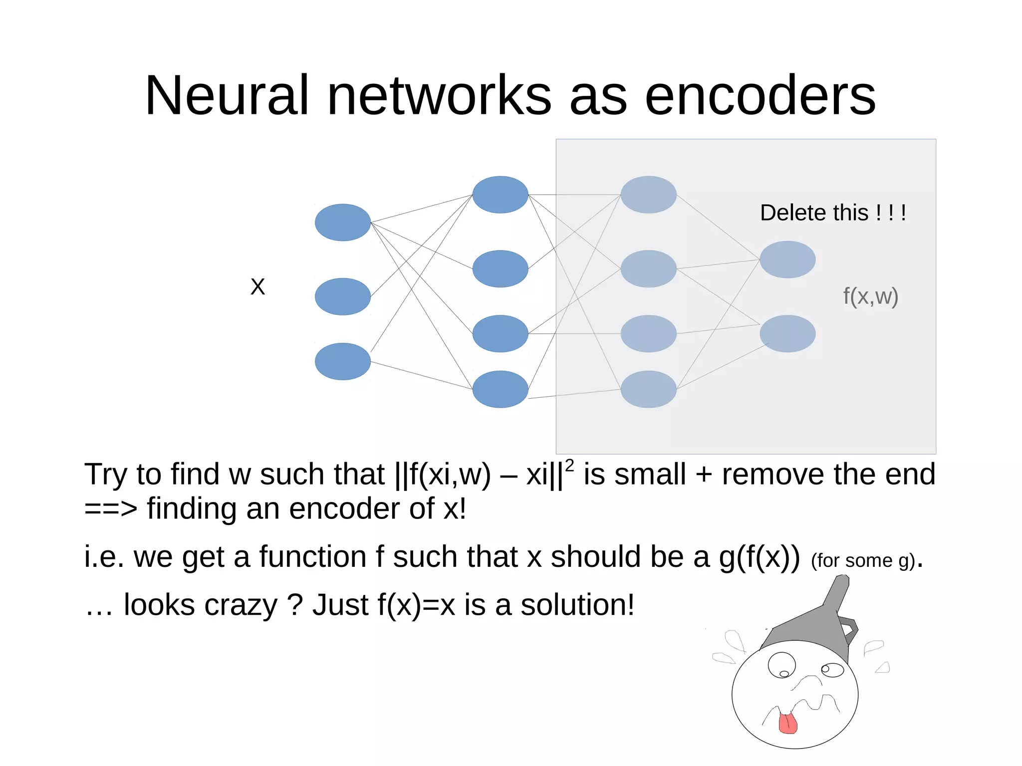
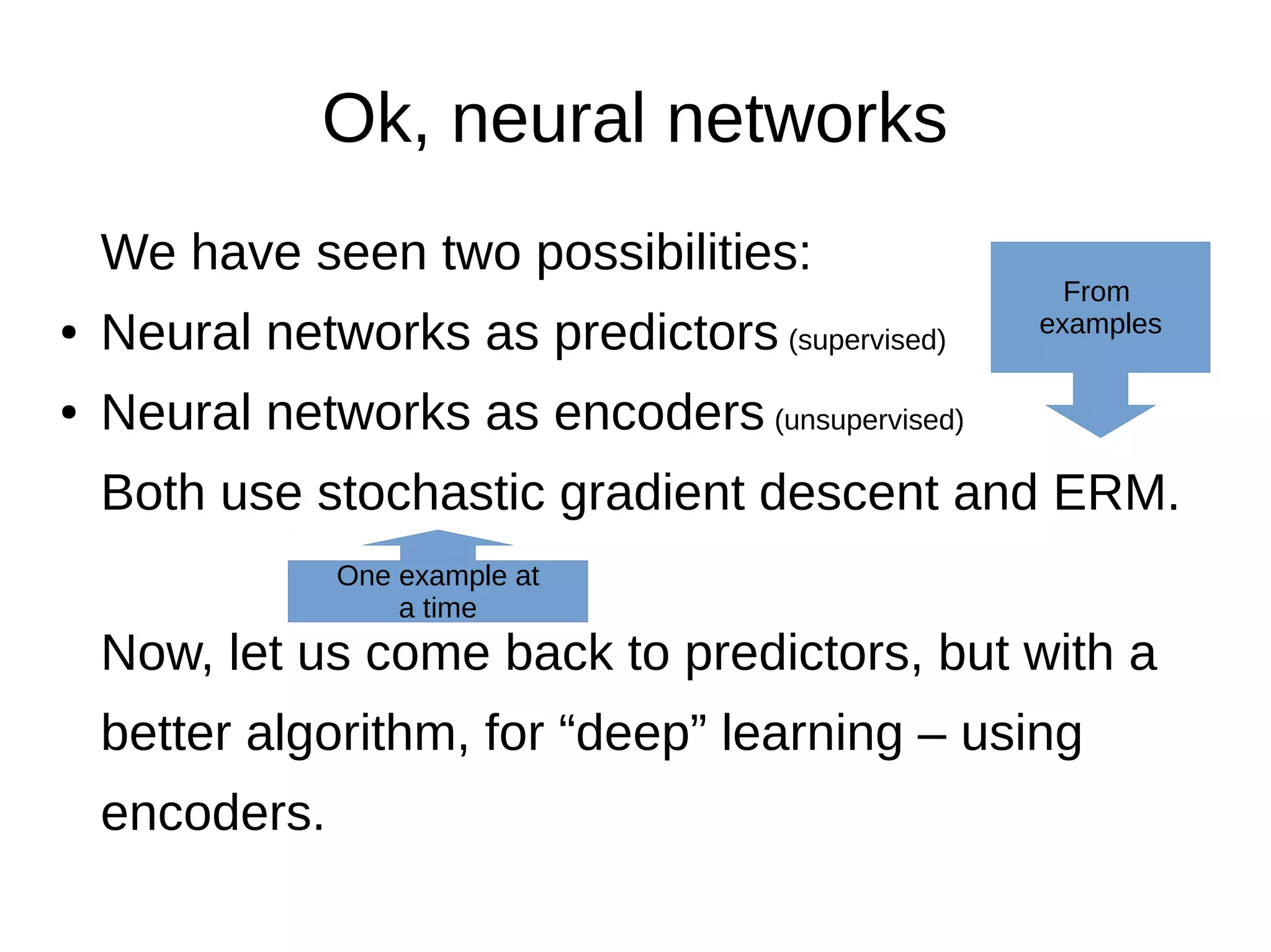
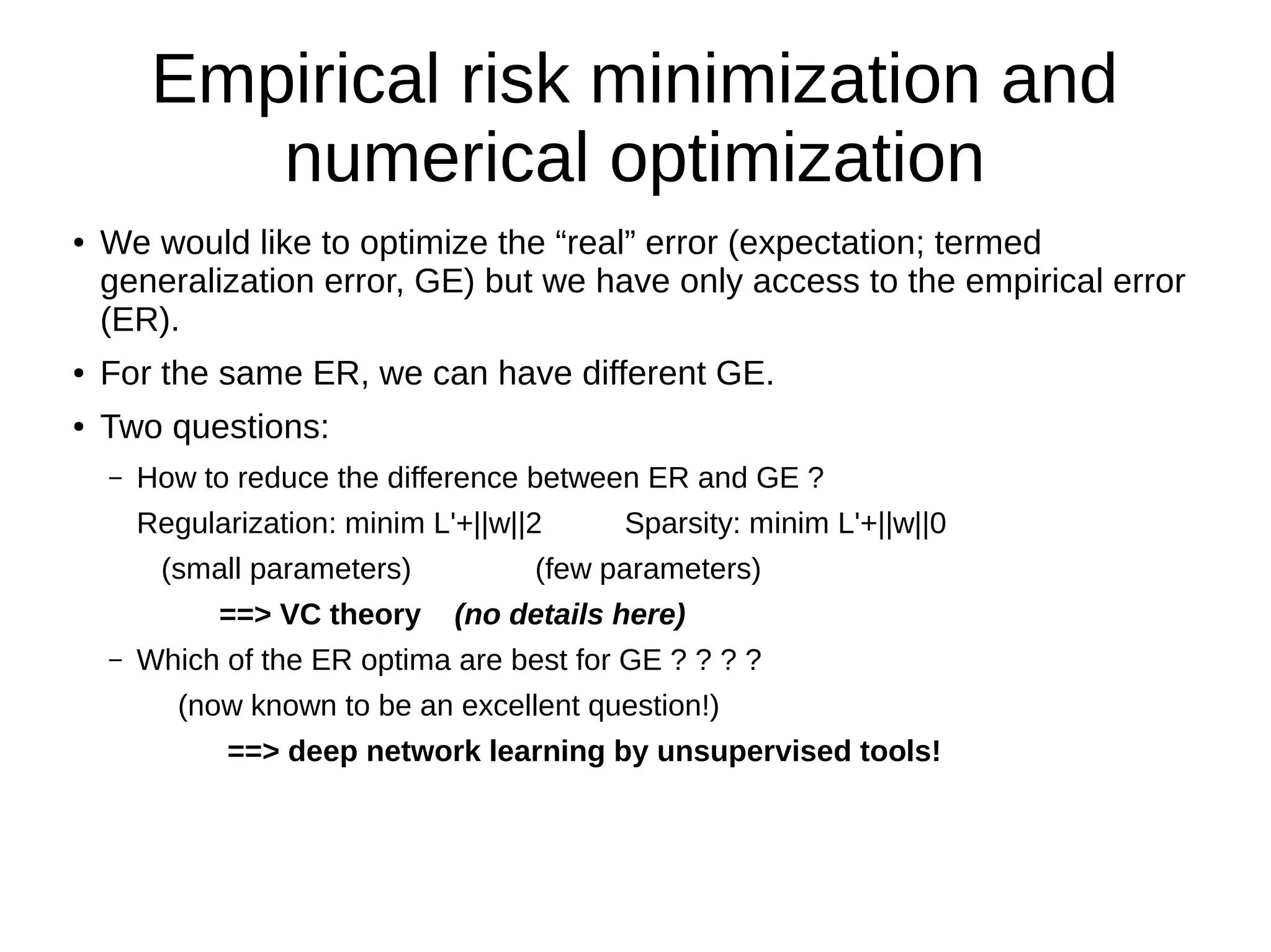
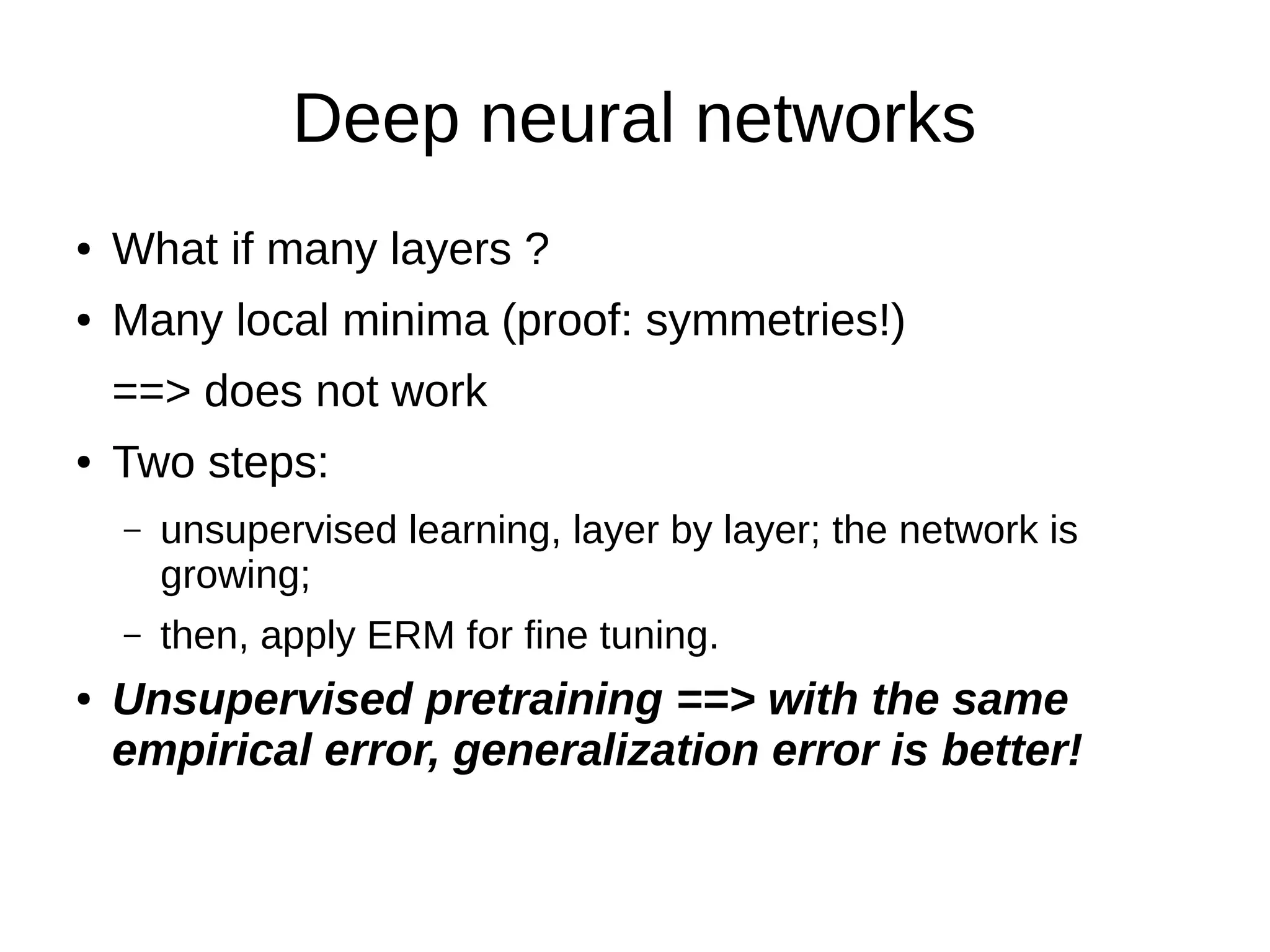
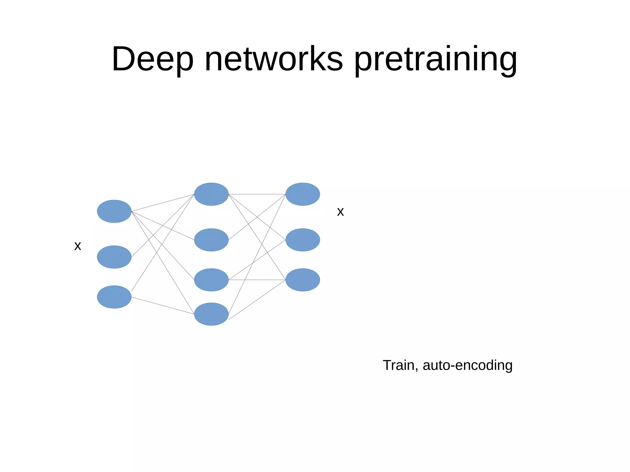
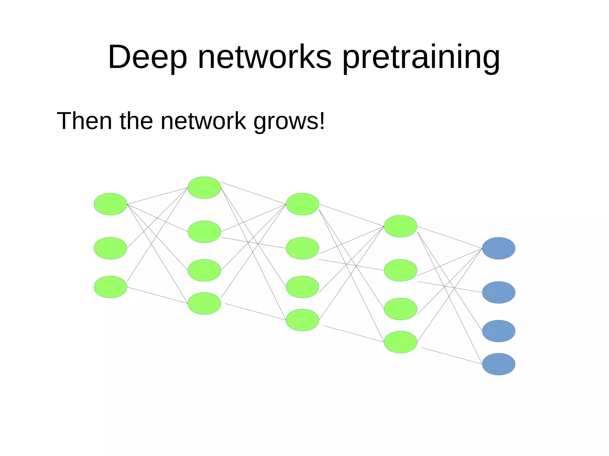
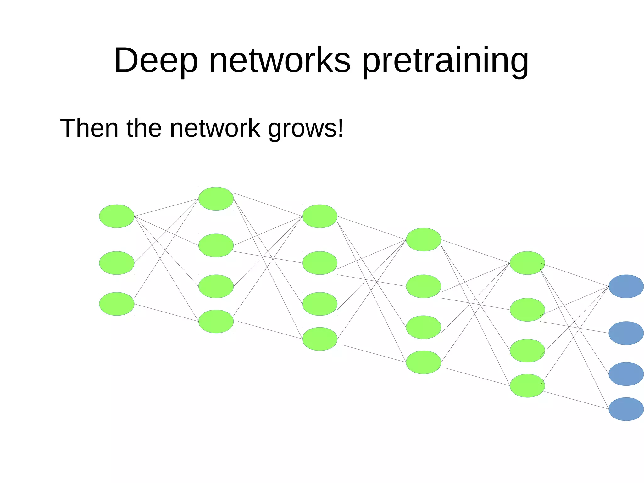
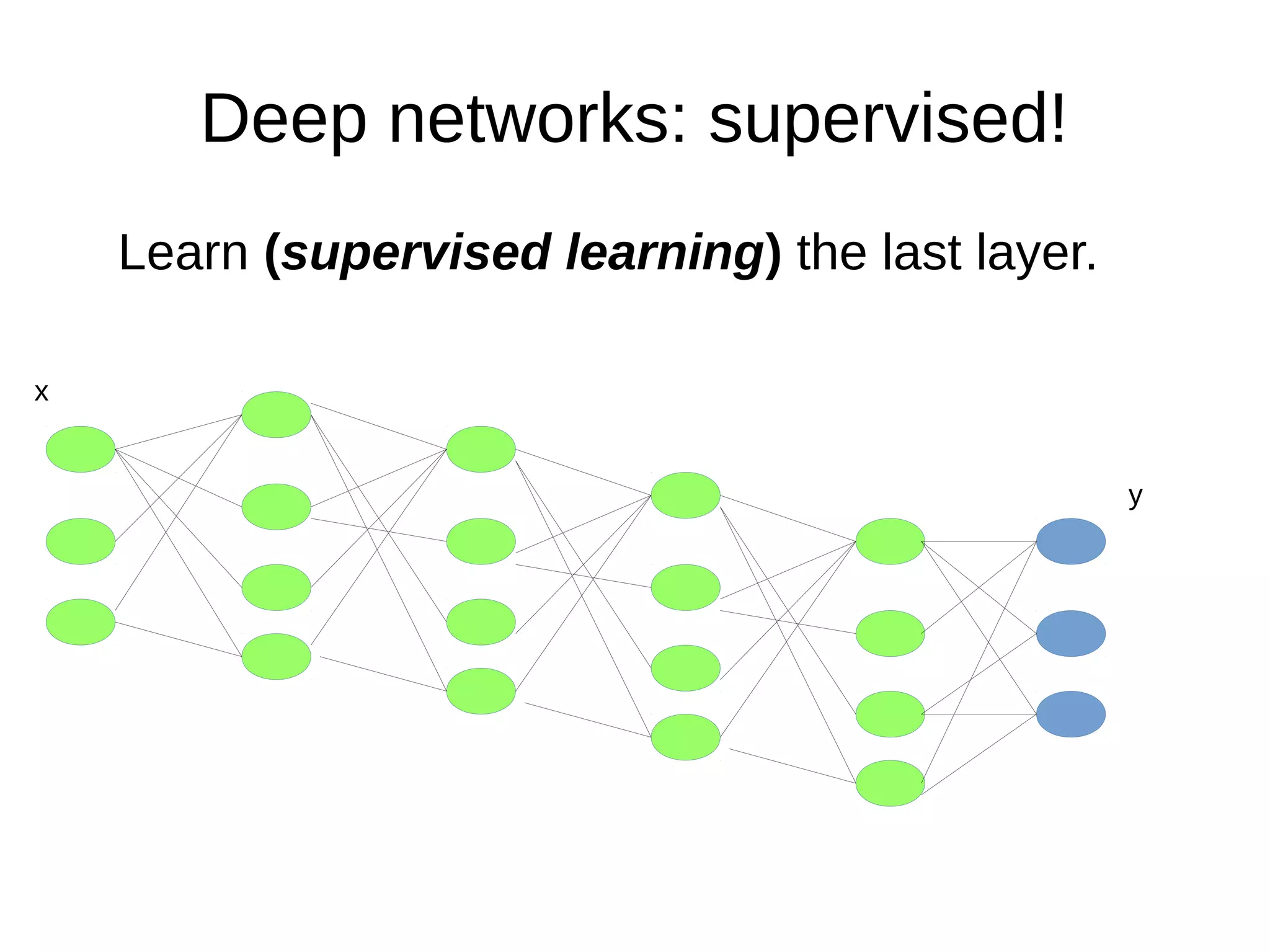
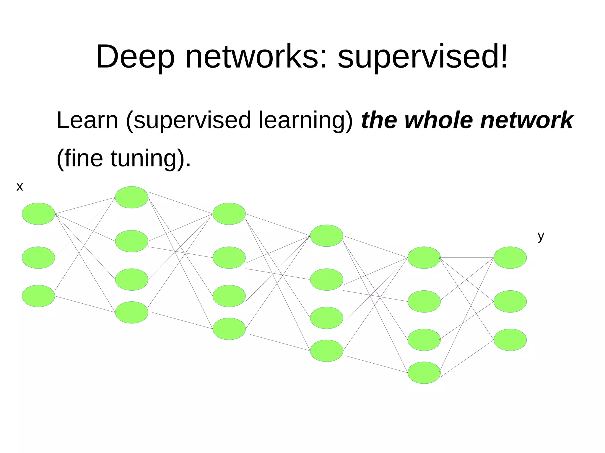


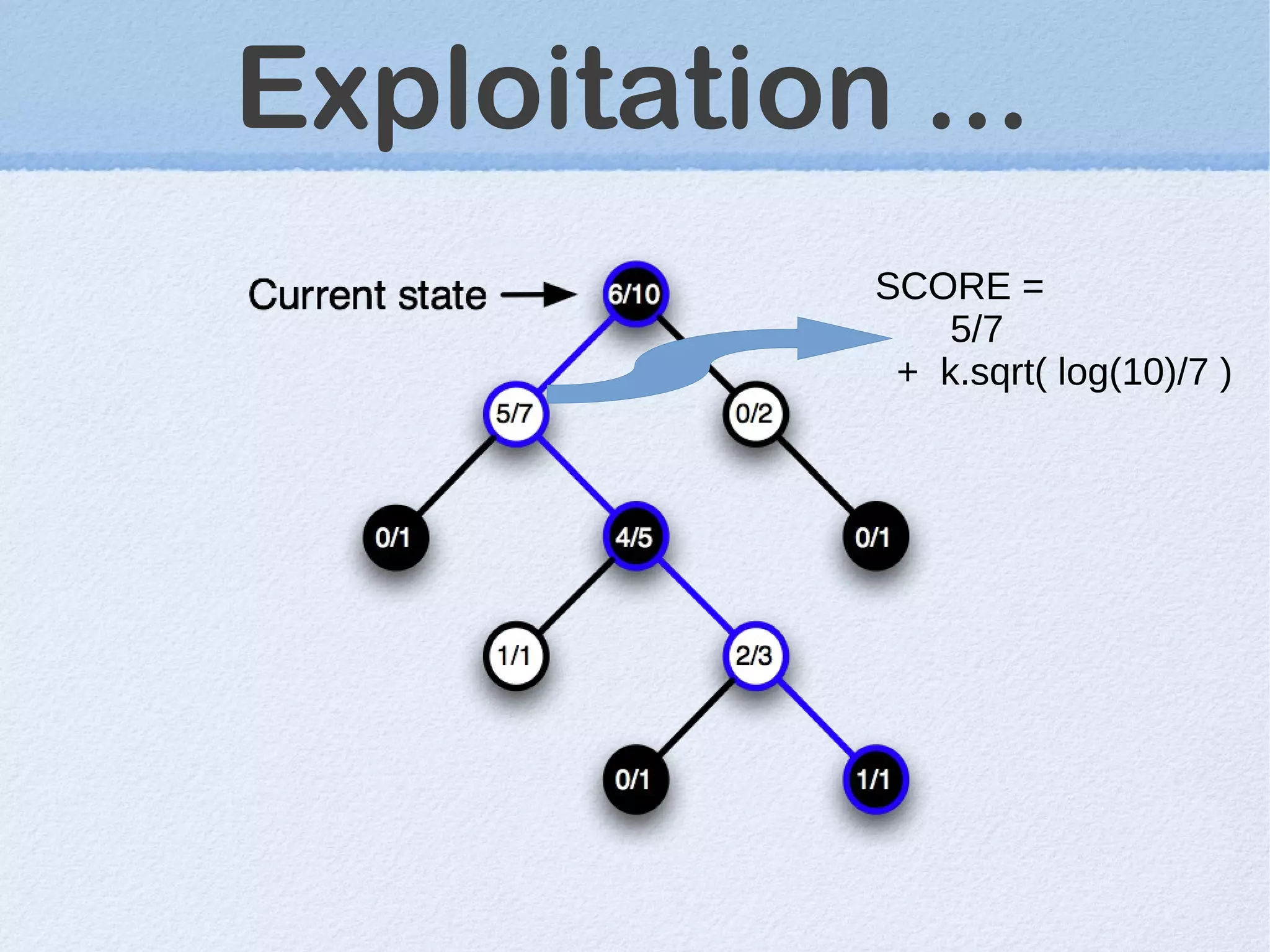
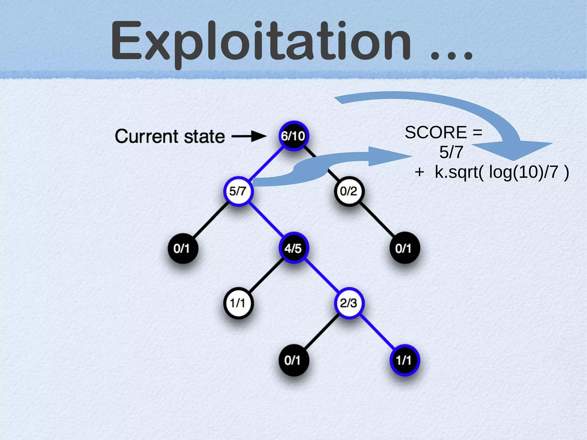
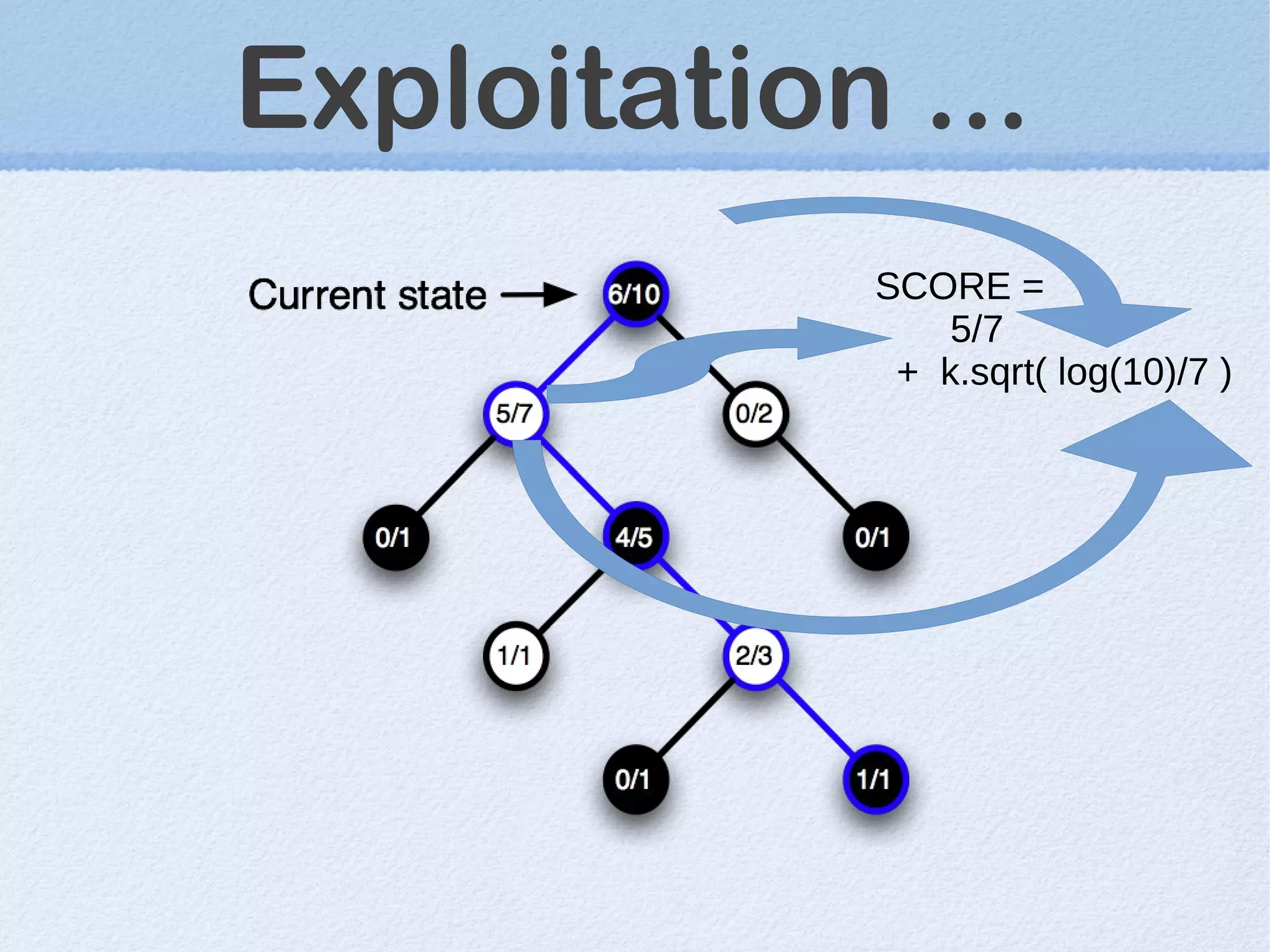
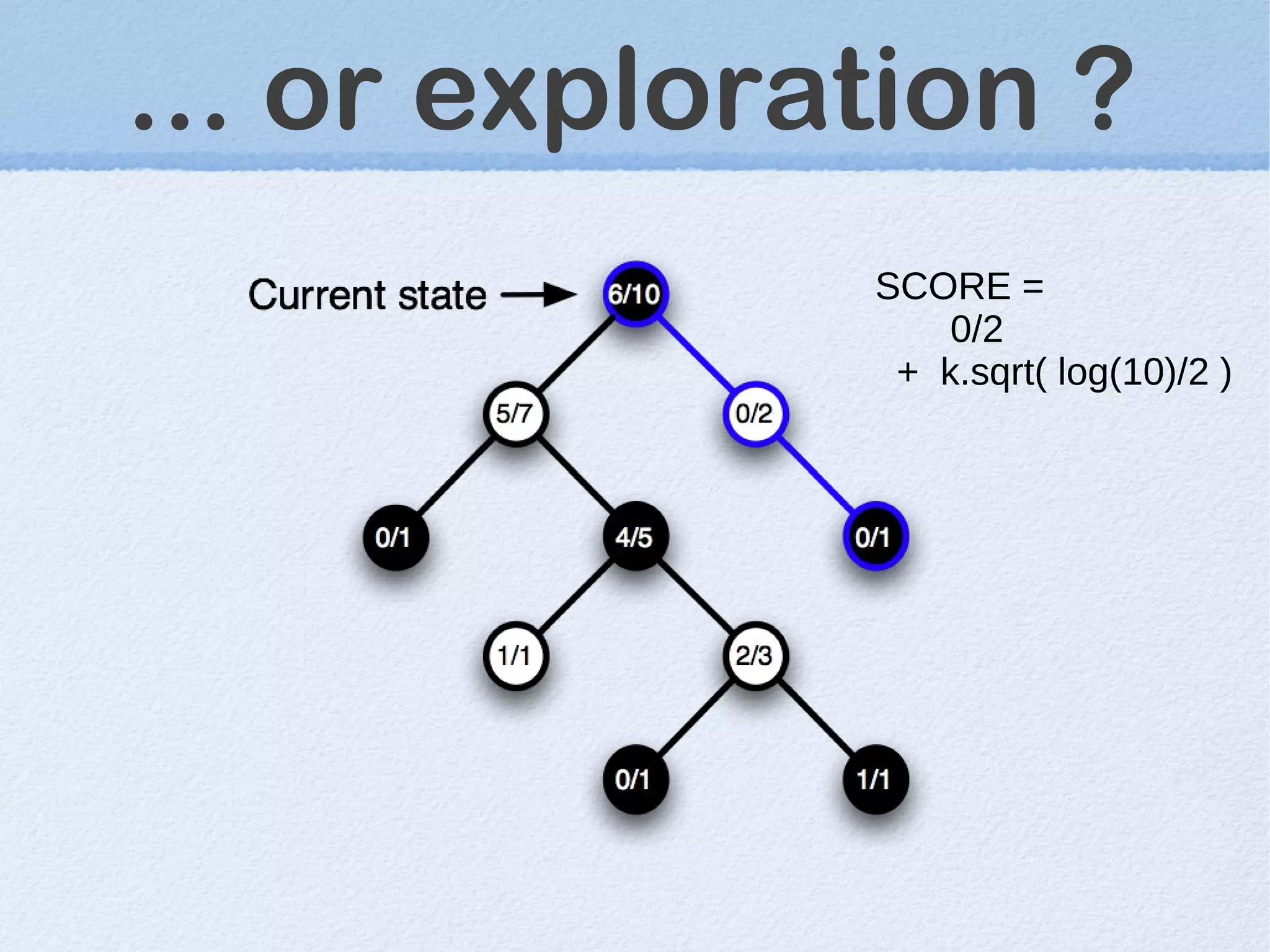
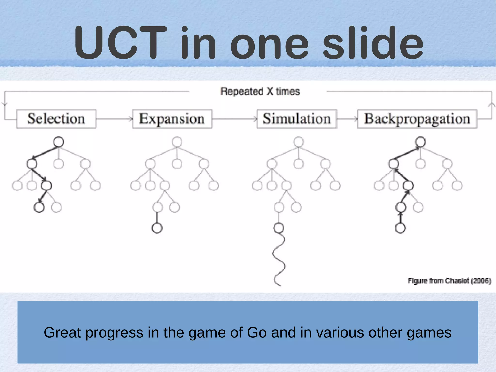


This document discusses machine learning (ML) concepts, emphasizing deep networks and Monte Carlo Tree Search (MCTS). It covers the fundamentals of ML, optimization techniques like stochastic gradient descent, and key algorithms such as deep learning for predictions and MCTS for games. The document concludes with insights on the significance of recent advancements, applications of ML, and the importance of foundational mathematics in the field.


![[update] Introductory Parts of the Book "Dive into Deep Learning"](https://cdn.slidesharecdn.com/ss_thumbnails/d2lq1introbasicssimplemodels-190415080926-thumbnail.jpg?width=640&height=640&fit=bounds)