Download as PDF, PPTX

![Forests of Trees
predictors
up
down
down
up
up
up
down
up
down
up
up
.
.
.
response
Y
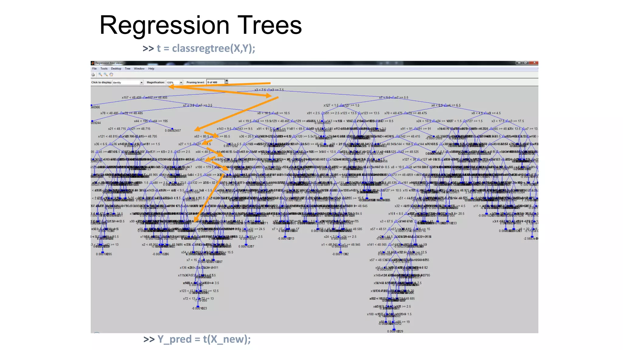
>> t = TreeBagger(nb_trees,X,Y);
>> [Y_pred,allpred] = predict(t,X_new);](https://image.slidesharecdn.com/machinelearningforfinance-140813050409-phpapp01/75/Machine-learning-for_finance-11-2048.jpg)
![Data Exploration: Getting an overview of individual
variables
Basic Histogram
>> hist(x(:,1))
Custom Number of Bins
>> hist(x(:,1),50)
By Group
>> hist(byGroup,20)
Gaussian fit
>> histfit(x(:,2))
3D Histogram
>> hist3(x(:,1:2))
Scatter Plot
>>gscatter(x(:,1),x(:,2),groups)
Pie Chart
>> pie3(proportions,groups)
>> X = [MPG,Acceleration,Displacement,Weight,Horsepower];
Box Plot
>> boxplot(x(:,1),groups)
5 10 15 20 25 30 35 40 45 50
0
10
20
30
40
50
60
70
80
5 10 15 20 25 30 35 40 45 50
0
5
10
15
20
25
6 8 10 12 14 16 18 20 22 24 26
0
10
20
30
40
50
60
5 10 15 20 25 30 35 40 45 50
8
10
12
14
16
18
20
22
24
26
3
4
5
6
8
10
15
20
25
30
35
40
45
3 4 5 6 8
5 10 15 20 25 30 35 40 45 50
0
5
10
15
20
25
byGroup(:,1)
byGroup(:,2)
Group6
Group5
Group8
Group3
Group4](https://image.slidesharecdn.com/machinelearningforfinance-140813050409-phpapp01/75/Machine-learning-for_finance-25-2048.jpg)
![Principal component analysis
1 2 3 4 5 6 7 8 9 10
0
0.005
0.01
0.015
0.02
0.0249
Principal Component
VarianceExplained(%)
0%
20%
40%
60%
80%
100%
-1
-0.5
0
0.5
1
-1
-0.5
0
0.5
1
-1
-0.5
0
0.5
1
Component 1
CommerzbankDeutscheBank
Infineon
ThyssenKruppMANDaimlerHeidelbergerAllianzDeutscheBahnBMWSalzgitterSiemensDeutschePostLufthansa
BASFAdidasMetroVWLindeEONMunichReBayerRWESAPMRKDeutscheTelekomBeiersdorf
Fresenius
HenkelFreseniusMedical
Component 2
Component3
>>[pcs,scrs,variances]=princomp(stocks);
-3 -2 -1 0 1 2 3
-2
0
2
-3
-2
-1
0
1
2
3](https://image.slidesharecdn.com/machinelearningforfinance-140813050409-phpapp01/75/Machine-learning-for_finance-27-2048.jpg)
![Factor model
Alternative to PCA to improve your components
>>[Lambda,Psi,T,stats,F]=factoran(stocks,3,'rotate','promax);
-1
-0.5
0
0.5
1 -1
-0.5
0
0.5
1
-1
-0.5
0
0.5
1
Component 2
DeutscheBank
DaimlerAllianzMAN
ThyssenKrupp
BMWLufthansa
Siemens
DeutschePost
Commerzbank
BASF
Adidas
Linde
MunichRe
MetroHeidelberger
SAP
Bayer
Salzgitter
Infineon
DeutscheBahn
EONRWE
VW
DeutscheTelekom
BeiersdorfMRKFresenius
Henkel
FreseniusMedical
Component 1
Component3](https://image.slidesharecdn.com/machinelearningforfinance-140813050409-phpapp01/75/Machine-learning-for_finance-28-2048.jpg)
![Paring predictors : stepwise optimization Some predictors might be correlated, other irrelevant
Requires Statistics Toolbox™
>>[coeff,inOut]=stepwisefit(stocks, index);
2007 2008 2009 2010 2011
-0.1
0
0.1
0.2
0.3
Returns
original data
stepwise fit
2007 2008 2009 2010 2011
0.5
1
1.5
Prices](https://image.slidesharecdn.com/machinelearningforfinance-140813050409-phpapp01/75/Machine-learning-for_finance-29-2048.jpg)
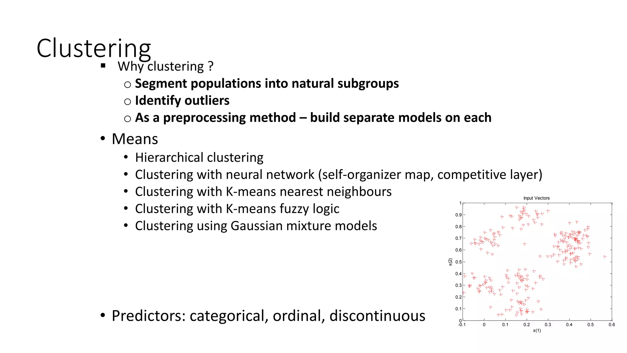
![Cloud of randomly generated points
• Each cluster center is randomly chosen inside specified bounds
• Each cluster contains the specified number of points per cluster
• Each cluster point is sampled from a gaussian distribution
• Multidimensionnal dataset
>>clusters = 8; % number of clusters.
>>points = 30; % number of points in each cluster.
>>std_dev = 0.05; % common cluster standard deviation
>>bounds = [0 1]; % bounds for the cluster center
>>[x,vcentroid,proportions,groups] =cluster_generation(bounds,clusters,points,std_dev);
-0.1 0 0.1 0.2 0.3 0.4 0.5 0.6
0
0.1
0.2
0.3
0.4
0.5
0.6
0.7
0.8
0.9
1
Group1
Group2
Group3
Group4
Group5
Group6
Group7
Group8](https://image.slidesharecdn.com/machinelearningforfinance-140813050409-phpapp01/75/Machine-learning-for_finance-30-2048.jpg)
![K-Means Cluster Analysis – how do I do it ?
Running the K-mean algorithm for K fixed
>> [memberships,centroids] = kmeans(x,K);
-0.1 0 0.1 0.2 0.3 0.4 0.5 0.6
0
0.1
0.2
0.3
0.4
0.5
0.6
0.7
0.8
0.9
1](https://image.slidesharecdn.com/machinelearningforfinance-140813050409-phpapp01/75/Machine-learning-for_finance-36-2048.jpg)
![Evaluating a K-Means analysis and choosing K
• Try a range of different K’s, and
compare the point-centroid
distances for each
>> for K=3:15
[clusters,centroids,distances] =
kmeans(data,K);
totaldist(K-2)=sum(distances);
end
plot(3:15,totaldist);
• Create silhouette plots
>> silhouette(data,clusters)](https://image.slidesharecdn.com/machinelearningforfinance-140813050409-phpapp01/75/Machine-learning-for_finance-37-2048.jpg)
![Fuzzy c-means Cluster Analysis – what is it doing?
• Very similar to K-means
• Samples are not assigned definitively to a cluster, but
have a ‘membership’ value relative to each cluster
Requires Fuzzy Logic Toolbox™
Running the fuzzy K-mean algorithm
for K fixed
>> [centroids, memberships]=fcm(x,K);](https://image.slidesharecdn.com/machinelearningforfinance-140813050409-phpapp01/75/Machine-learning-for_finance-39-2048.jpg)
![Gaussian Mixture Models
• Assume that data is drawn from a fixed number K of normal
distributions
• Fit these parameters using the EM algorithm
>> gmobj = gmdistribution.fit(x,8);
>> assignments = cluster(gmobj,x);
Plot the probability density
>> ezsurf(@(x,y)pdf(gmobj,[x y]));
0
0.2
0.4
0.6
0.8
1
0.2
0.4
0.6
0.8
1
0
10
20](https://image.slidesharecdn.com/machinelearningforfinance-140813050409-phpapp01/75/Machine-learning-for_finance-40-2048.jpg)
![Evaluating a Gaussian Mixture Model clustering
• Plot the probability density function of the model
>> ezsurf(@(x,y)pdf(gmobj,[x y]));
• Plot the posterior probabilities of observations
>> p = posterior(gmobj,data);
>> scatter(data(:,1),data(:,2),5,p(:,g)); % Do this for each group g
• Plot the Mahalanobis distances of observations to components
>> m = mahal(gmobj,data);
>> scatter(data(:,1),data(:,2),5,m(:,g)); % Do this for each group g](https://image.slidesharecdn.com/machinelearningforfinance-140813050409-phpapp01/75/Machine-learning-for_finance-41-2048.jpg)

![Interpreting Discriminant Analyses
• Visualise the posterior probability
surfaces
>> [XI,YI] = meshgrid(linspace(4,8),
linspace(2,4.5));
>> X = XI(:); Y = YI(:);
>> [class,err,P] = classify([X Y],
meas(:,1:2), species,'quadratic');
>> for i=1:3
ZI = reshape(P(:,i),100,100);
surf(XI,YI,ZI,'EdgeColor','none');
hold on;
end](https://image.slidesharecdn.com/machinelearningforfinance-140813050409-phpapp01/75/Machine-learning-for_finance-49-2048.jpg)
![Interpreting Discriminant Analyses
• Visualise the probability density
of sample observations
• An indicator of the region in
which the model has support
from training data
>> [XI,YI] = meshgrid(linspace(4,8),
linspace(2,4.5));
>> X = XI(:); Y = YI(:);
>> [class,err,P,logp] = classify([X Y],
meas(:,1:2), species, 'quadratic');
>> ZI = reshape(logp,100,100);
>> surf(XI,YI,ZI,'EdgeColor','none');](https://image.slidesharecdn.com/machinelearningforfinance-140813050409-phpapp01/75/Machine-learning-for_finance-50-2048.jpg)
![Enhancing the model : bagged trees
• Prune the decision tree
>> [cost,secost,ntnodes,bestlevel] =test(t, 'test', x, y);
>> topt = prune(t, 'level', bestlevel);
• Bootstrapped aggregated trees forest
>> [cost,secost,ntnodes,bestlevel] =test(t, 'test', x, y);
>> forest = TreeBagger(100, x, y);
>> y_pred = predict(forest,x);
• Visualise class boundaries as before
-0.4 -0.2 0 0.2 0.4 0.6 0.8 1 1.2 1.4 1.6
-0.5
0
0.5
1
1.5
x1
x2
group1
group2
group3
group4
group5
group6
group7
group8](https://image.slidesharecdn.com/machinelearningforfinance-140813050409-phpapp01/75/Machine-learning-for_finance-54-2048.jpg)
![Pattern Recognition Neural Network– how do I
build them ?
• Build a neural network model
>> net = patternnet(10);
• Train the net to classify
observations
>> [net,tr] = train(net,x,y);
• Apply the model to new data
>> y_pred = net(x);
0 0.2 0.4 0.6 0.8 1
0
0.2
0.4
0.6
0.8
1
x1
x2
1
2
3
4
5
6
7
8](https://image.slidesharecdn.com/machinelearningforfinance-140813050409-phpapp01/75/Machine-learning-for_finance-56-2048.jpg)
![New data set with a continuous response from one
predictor
• Non-linear function to fit
• A continuous response to fit from one continuous predictor
>>[x,t] = simplefit_dataset;
0 1 2 3 4 5 6 7 8 9 10
0
1
2
3
4
5
6
7
8
9
10](https://image.slidesharecdn.com/machinelearningforfinance-140813050409-phpapp01/75/Machine-learning-for_finance-62-2048.jpg)
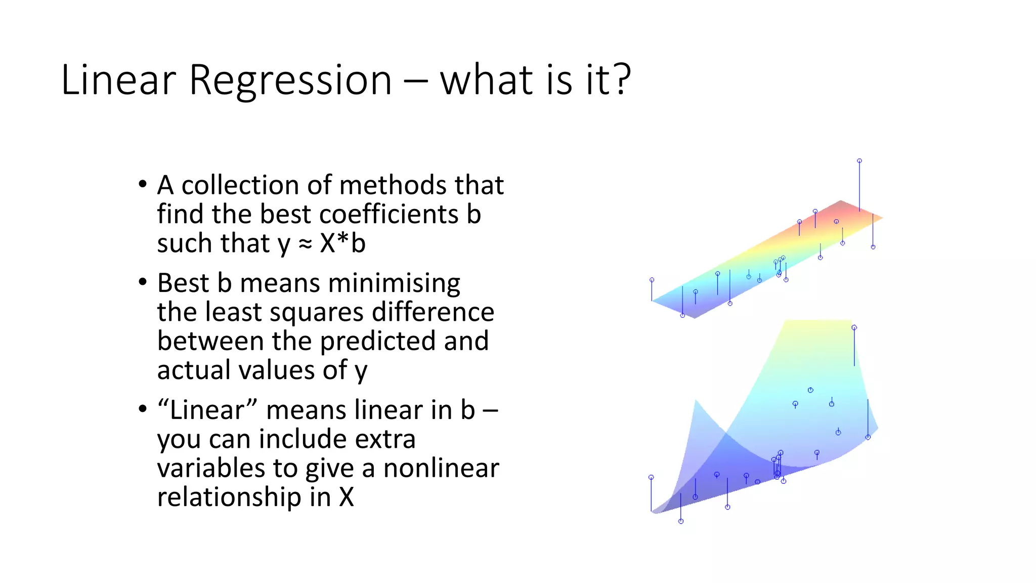
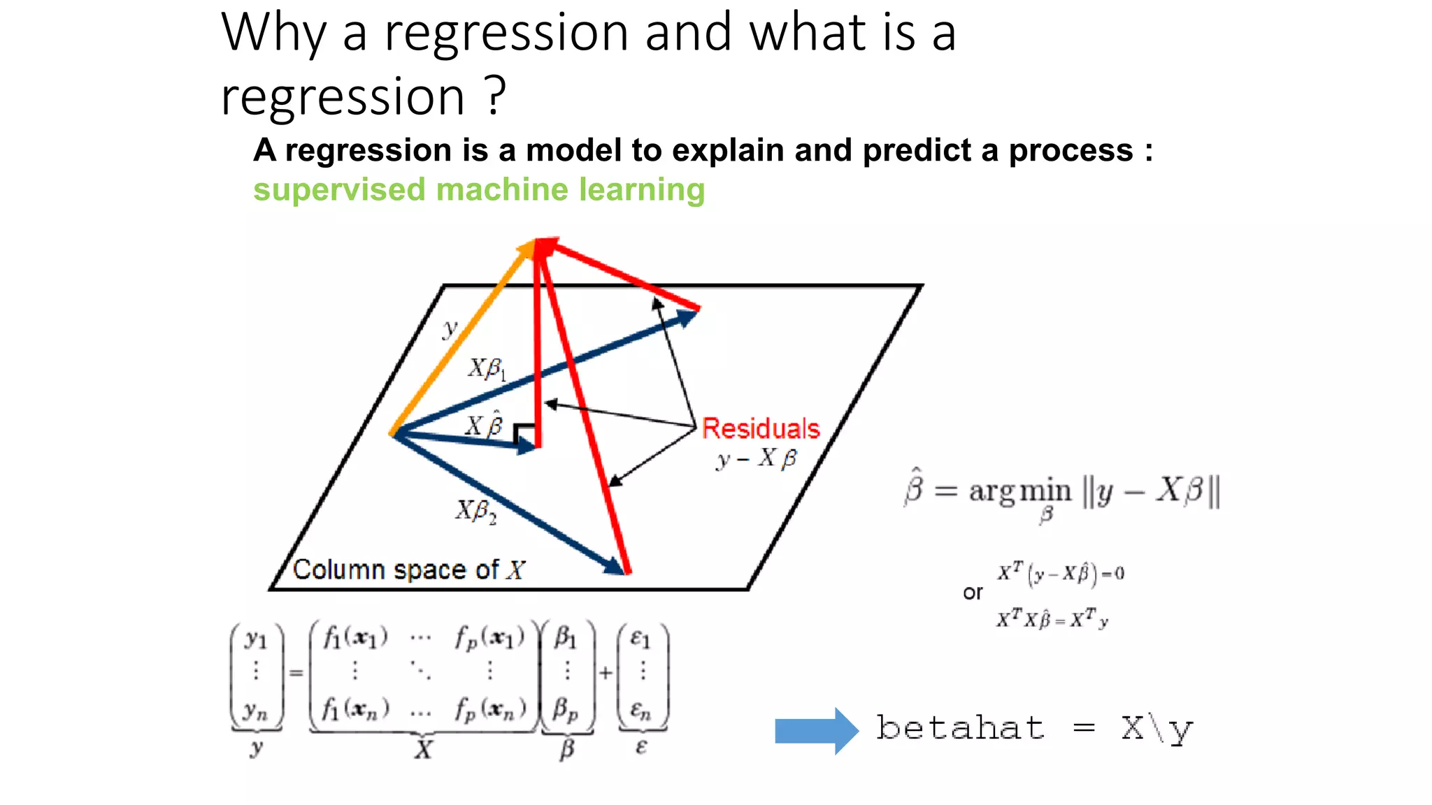
![Linear Regression – how do I do it ?
>> b = xy
• Linear Regression
>> b = regress(y, [ones(size(X,1),1) x])
>> stats = regstats(y, [ones(size(x,1),1) x])
• Robust Regression – better in the presence of outliers
>> robust_b = robustfit(X,y) %NB (X,y) not (y,X)
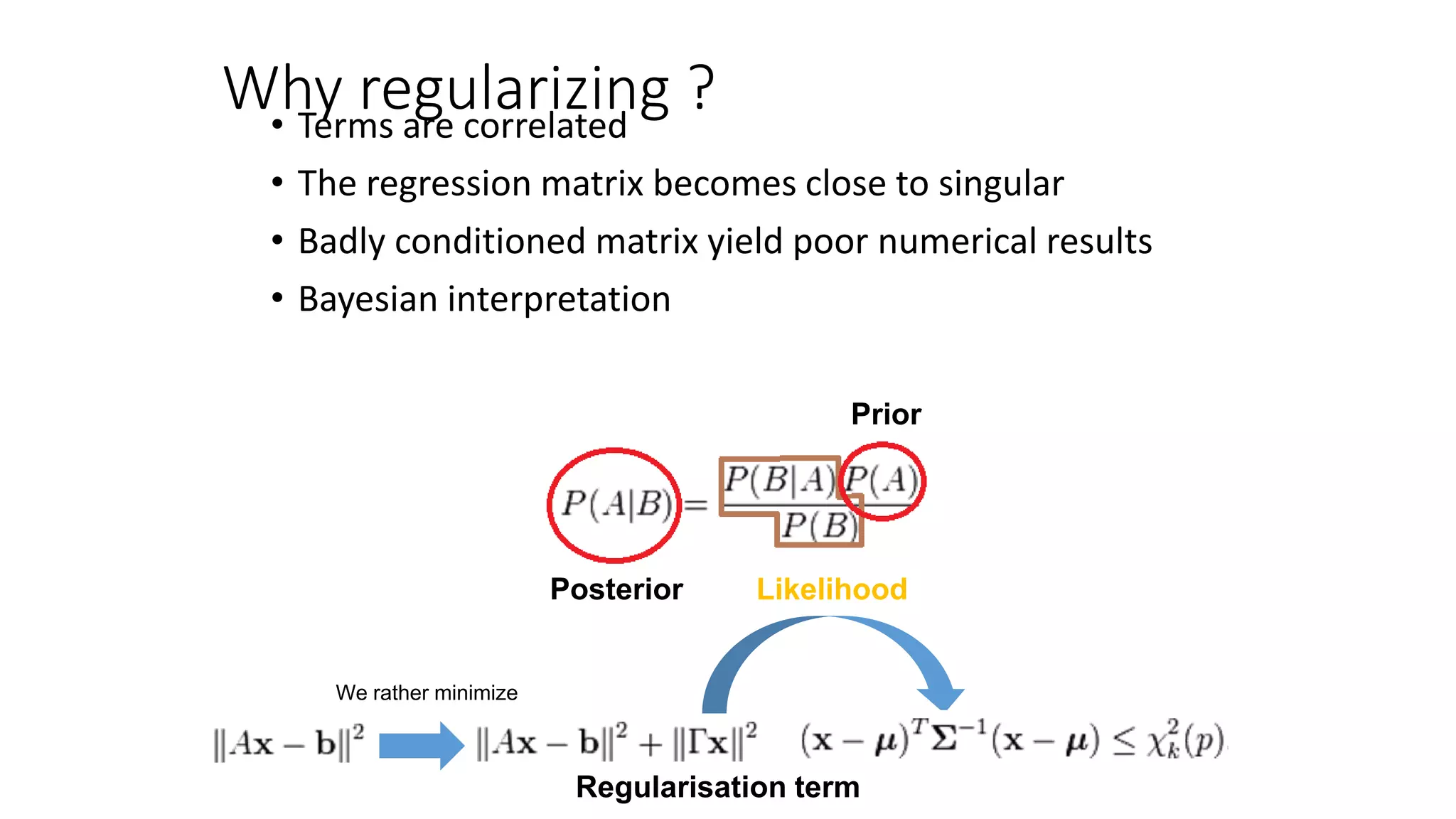
• Ridge Regression – better if data is close to collinear
>> ridge_b = ridge(y,X,k) %k is the ridge parameter
• Apply the model to new data
>> y = newdata*b;](https://image.slidesharecdn.com/machinelearningforfinance-140813050409-phpapp01/75/Machine-learning-for_finance-64-2048.jpg)
![Interpreting a linear regression model
• Examine coefficients to see
which predictors have a large
effect on the response
>> [b,bint,r,rint,stats]=regress(y,X)
>> errorbar(1:size(b,1),b, b-
bint(:,1),bint(:,2)-b)
• Examine residuals to check for
possible outliers
>> rcoplot(r,rint)
• Examine R2 statistic and p-
value to check overall model
significance
>> stats(1)*100 %R2 as a percentage
>> stats(3) %p-value
• Additional diagnostics with
regstats](https://image.slidesharecdn.com/machinelearningforfinance-140813050409-phpapp01/75/Machine-learning-for_finance-65-2048.jpg)
![Non linear curve fitting
Least square algorithm
>> model = @(b,x)(b(1)+b(2).*cos(b(3)*x+b(4))+b(5).*cos(b(6)*x+b(7))+b(8).*cos(b(9)*x+b(10)));
>> [ahat,r,J,cov,mse] = nlinfit(x,t,model,a0);
0 1 2 3 4 5 6 7 8 9 10
-5
0
5
10
15
0 10 20 30 40 50 60 70 80 90 100
0
0.05
0.1
0.15
0.2](https://image.slidesharecdn.com/machinelearningforfinance-140813050409-phpapp01/75/Machine-learning-for_finance-66-2048.jpg)
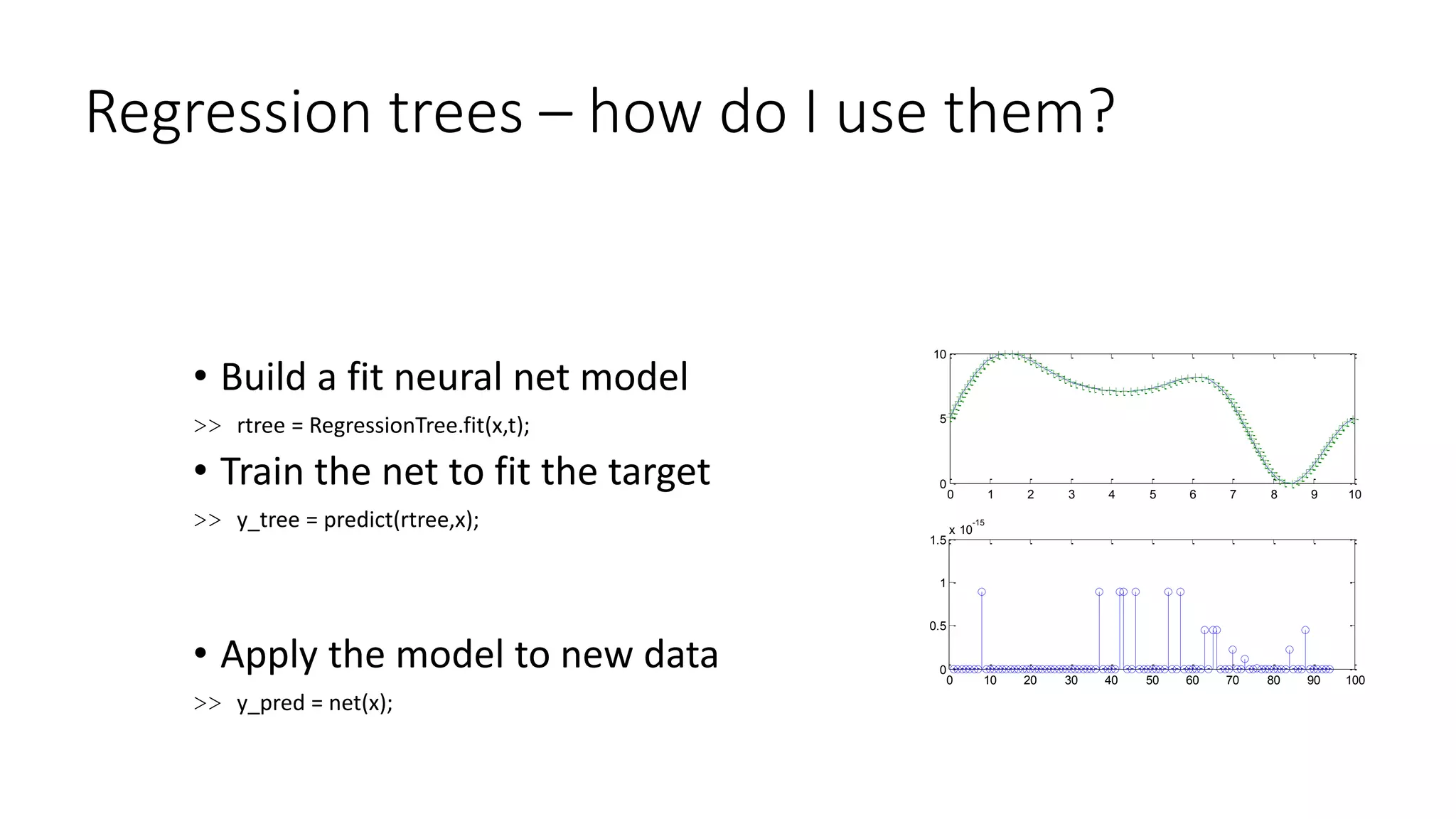
![Fit Neural Network– how do I build them ?
• Build a fit neural net model
>> net = fitnet(10);
• Train the net to fit the target
>> [net,tr] = train(net,x,t);
• Apply the model to new data
>> y_pred = net(x);
0 1 2 3 4 5 6 7 8 9
-2
0
2
4
6
8
10
12
Function Fit for Output Element 1
OutputandTarget
-0.02
0
0.02
0.04
Error
Input
Targets
Outputs
Errors
Fit
Targets - Outputs](https://image.slidesharecdn.com/machinelearningforfinance-140813050409-phpapp01/75/Machine-learning-for_finance-68-2048.jpg)


![Forests of Trees
predictors
up
down
down
up
up
up
down
up
down
up
up
.
.
.
response
Y
>> t = TreeBagger(nb_trees,X,Y);
>> [Y_pred,allpred] = predict(t,X_new);](https://crownmelresort.com/image.slidesharecdn.com/machinelearningforfinance-140813050409-phpapp01/75/Machine-learning-for_finance-11-2048.jpg)


![Data Exploration: Getting an overview of individual
variables
Basic Histogram
>> hist(x(:,1))
Custom Number of Bins
>> hist(x(:,1),50)
By Group
>> hist(byGroup,20)
Gaussian fit
>> histfit(x(:,2))
3D Histogram
>> hist3(x(:,1:2))
Scatter Plot
>>gscatter(x(:,1),x(:,2),groups)
Pie Chart
>> pie3(proportions,groups)
>> X = [MPG,Acceleration,Displacement,Weight,Horsepower];
Box Plot
>> boxplot(x(:,1),groups)
5 10 15 20 25 30 35 40 45 50
0
10
20
30
40
50
60
70
80
5 10 15 20 25 30 35 40 45 50
0
5
10
15
20
25
6 8 10 12 14 16 18 20 22 24 26
0
10
20
30
40
50
60
5 10 15 20 25 30 35 40 45 50
8
10
12
14
16
18
20
22
24
26
3
4
5
6
8
10
15
20
25
30
35
40
45
3 4 5 6 8
5 10 15 20 25 30 35 40 45 50
0
5
10
15
20
25
byGroup(:,1)
byGroup(:,2)
Group6
Group5
Group8
Group3
Group4](https://crownmelresort.com/image.slidesharecdn.com/machinelearningforfinance-140813050409-phpapp01/75/Machine-learning-for_finance-25-2048.jpg)

![Principal component analysis
1 2 3 4 5 6 7 8 9 10
0
0.005
0.01
0.015
0.02
0.0249
Principal Component
VarianceExplained(%)
0%
20%
40%
60%
80%
100%
-1
-0.5
0
0.5
1
-1
-0.5
0
0.5
1
-1
-0.5
0
0.5
1
Component 1
CommerzbankDeutscheBank
Infineon
ThyssenKruppMANDaimlerHeidelbergerAllianzDeutscheBahnBMWSalzgitterSiemensDeutschePostLufthansa
BASFAdidasMetroVWLindeEONMunichReBayerRWESAPMRKDeutscheTelekomBeiersdorf
Fresenius
HenkelFreseniusMedical
Component 2
Component3
>>[pcs,scrs,variances]=princomp(stocks);
-3 -2 -1 0 1 2 3
-2
0
2
-3
-2
-1
0
1
2
3](https://crownmelresort.com/image.slidesharecdn.com/machinelearningforfinance-140813050409-phpapp01/75/Machine-learning-for_finance-27-2048.jpg)
![Factor model
Alternative to PCA to improve your components
>>[Lambda,Psi,T,stats,F]=factoran(stocks,3,'rotate','promax);
-1
-0.5
0
0.5
1 -1
-0.5
0
0.5
1
-1
-0.5
0
0.5
1
Component 2
DeutscheBank
DaimlerAllianzMAN
ThyssenKrupp
BMWLufthansa
Siemens
DeutschePost
Commerzbank
BASF
Adidas
Linde
MunichRe
MetroHeidelberger
SAP
Bayer
Salzgitter
Infineon
DeutscheBahn
EONRWE
VW
DeutscheTelekom
BeiersdorfMRKFresenius
Henkel
FreseniusMedical
Component 1
Component3](https://crownmelresort.com/image.slidesharecdn.com/machinelearningforfinance-140813050409-phpapp01/75/Machine-learning-for_finance-28-2048.jpg)
![Paring predictors : stepwise optimization Some predictors might be correlated, other irrelevant
Requires Statistics Toolbox™
>>[coeff,inOut]=stepwisefit(stocks, index);
2007 2008 2009 2010 2011
-0.1
0
0.1
0.2
0.3
Returns
original data
stepwise fit
2007 2008 2009 2010 2011
0.5
1
1.5
Prices](https://crownmelresort.com/image.slidesharecdn.com/machinelearningforfinance-140813050409-phpapp01/75/Machine-learning-for_finance-29-2048.jpg)
![Cloud of randomly generated points
• Each cluster center is randomly chosen inside specified bounds
• Each cluster contains the specified number of points per cluster
• Each cluster point is sampled from a gaussian distribution
• Multidimensionnal dataset
>>clusters = 8; % number of clusters.
>>points = 30; % number of points in each cluster.
>>std_dev = 0.05; % common cluster standard deviation
>>bounds = [0 1]; % bounds for the cluster center
>>[x,vcentroid,proportions,groups] =cluster_generation(bounds,clusters,points,std_dev);
-0.1 0 0.1 0.2 0.3 0.4 0.5 0.6
0
0.1
0.2
0.3
0.4
0.5
0.6
0.7
0.8
0.9
1
Group1
Group2
Group3
Group4
Group5
Group6
Group7
Group8](https://crownmelresort.com/image.slidesharecdn.com/machinelearningforfinance-140813050409-phpapp01/75/Machine-learning-for_finance-30-2048.jpg)


![K-Means Cluster Analysis – how do I do it ?
Running the K-mean algorithm for K fixed
>> [memberships,centroids] = kmeans(x,K);
-0.1 0 0.1 0.2 0.3 0.4 0.5 0.6
0
0.1
0.2
0.3
0.4
0.5
0.6
0.7
0.8
0.9
1](https://crownmelresort.com/image.slidesharecdn.com/machinelearningforfinance-140813050409-phpapp01/75/Machine-learning-for_finance-36-2048.jpg)
![Evaluating a K-Means analysis and choosing K
• Try a range of different K’s, and
compare the point-centroid
distances for each
>> for K=3:15
[clusters,centroids,distances] =
kmeans(data,K);
totaldist(K-2)=sum(distances);
end
plot(3:15,totaldist);
• Create silhouette plots
>> silhouette(data,clusters)](https://crownmelresort.com/image.slidesharecdn.com/machinelearningforfinance-140813050409-phpapp01/75/Machine-learning-for_finance-37-2048.jpg)

![Fuzzy c-means Cluster Analysis – what is it doing?
• Very similar to K-means
• Samples are not assigned definitively to a cluster, but
have a ‘membership’ value relative to each cluster
Requires Fuzzy Logic Toolbox™
Running the fuzzy K-mean algorithm
for K fixed
>> [centroids, memberships]=fcm(x,K);](https://crownmelresort.com/image.slidesharecdn.com/machinelearningforfinance-140813050409-phpapp01/75/Machine-learning-for_finance-39-2048.jpg)
![Gaussian Mixture Models
• Assume that data is drawn from a fixed number K of normal
distributions
• Fit these parameters using the EM algorithm
>> gmobj = gmdistribution.fit(x,8);
>> assignments = cluster(gmobj,x);
Plot the probability density
>> ezsurf(@(x,y)pdf(gmobj,[x y]));
0
0.2
0.4
0.6
0.8
1
0.2
0.4
0.6
0.8
1
0
10
20](https://crownmelresort.com/image.slidesharecdn.com/machinelearningforfinance-140813050409-phpapp01/75/Machine-learning-for_finance-40-2048.jpg)
![Evaluating a Gaussian Mixture Model clustering
• Plot the probability density function of the model
>> ezsurf(@(x,y)pdf(gmobj,[x y]));
• Plot the posterior probabilities of observations
>> p = posterior(gmobj,data);
>> scatter(data(:,1),data(:,2),5,p(:,g)); % Do this for each group g
• Plot the Mahalanobis distances of observations to components
>> m = mahal(gmobj,data);
>> scatter(data(:,1),data(:,2),5,m(:,g)); % Do this for each group g](https://crownmelresort.com/image.slidesharecdn.com/machinelearningforfinance-140813050409-phpapp01/75/Machine-learning-for_finance-41-2048.jpg)


![Interpreting Discriminant Analyses
• Visualise the posterior probability
surfaces
>> [XI,YI] = meshgrid(linspace(4,8),
linspace(2,4.5));
>> X = XI(:); Y = YI(:);
>> [class,err,P] = classify([X Y],
meas(:,1:2), species,'quadratic');
>> for i=1:3
ZI = reshape(P(:,i),100,100);
surf(XI,YI,ZI,'EdgeColor','none');
hold on;
end](https://crownmelresort.com/image.slidesharecdn.com/machinelearningforfinance-140813050409-phpapp01/75/Machine-learning-for_finance-49-2048.jpg)
![Interpreting Discriminant Analyses
• Visualise the probability density
of sample observations
• An indicator of the region in
which the model has support
from training data
>> [XI,YI] = meshgrid(linspace(4,8),
linspace(2,4.5));
>> X = XI(:); Y = YI(:);
>> [class,err,P,logp] = classify([X Y],
meas(:,1:2), species, 'quadratic');
>> ZI = reshape(logp,100,100);
>> surf(XI,YI,ZI,'EdgeColor','none');](https://crownmelresort.com/image.slidesharecdn.com/machinelearningforfinance-140813050409-phpapp01/75/Machine-learning-for_finance-50-2048.jpg)


![Enhancing the model : bagged trees
• Prune the decision tree
>> [cost,secost,ntnodes,bestlevel] =test(t, 'test', x, y);
>> topt = prune(t, 'level', bestlevel);
• Bootstrapped aggregated trees forest
>> [cost,secost,ntnodes,bestlevel] =test(t, 'test', x, y);
>> forest = TreeBagger(100, x, y);
>> y_pred = predict(forest,x);
• Visualise class boundaries as before
-0.4 -0.2 0 0.2 0.4 0.6 0.8 1 1.2 1.4 1.6
-0.5
0
0.5
1
1.5
x1
x2
group1
group2
group3
group4
group5
group6
group7
group8](https://crownmelresort.com/image.slidesharecdn.com/machinelearningforfinance-140813050409-phpapp01/75/Machine-learning-for_finance-54-2048.jpg)

![Pattern Recognition Neural Network– how do I
build them ?
• Build a neural network model
>> net = patternnet(10);
• Train the net to classify
observations
>> [net,tr] = train(net,x,y);
• Apply the model to new data
>> y_pred = net(x);
0 0.2 0.4 0.6 0.8 1
0
0.2
0.4
0.6
0.8
1
x1
x2
1
2
3
4
5
6
7
8](https://crownmelresort.com/image.slidesharecdn.com/machinelearningforfinance-140813050409-phpapp01/75/Machine-learning-for_finance-56-2048.jpg)


![New data set with a continuous response from one
predictor
• Non-linear function to fit
• A continuous response to fit from one continuous predictor
>>[x,t] = simplefit_dataset;
0 1 2 3 4 5 6 7 8 9 10
0
1
2
3
4
5
6
7
8
9
10](https://crownmelresort.com/image.slidesharecdn.com/machinelearningforfinance-140813050409-phpapp01/75/Machine-learning-for_finance-62-2048.jpg)

![Linear Regression – how do I do it ?
>> b = xy
• Linear Regression
>> b = regress(y, [ones(size(X,1),1) x])
>> stats = regstats(y, [ones(size(x,1),1) x])
• Robust Regression – better in the presence of outliers
>> robust_b = robustfit(X,y) %NB (X,y) not (y,X)
• Ridge Regression – better if data is close to collinear
>> ridge_b = ridge(y,X,k) %k is the ridge parameter
• Apply the model to new data
>> y = newdata*b;](https://crownmelresort.com/image.slidesharecdn.com/machinelearningforfinance-140813050409-phpapp01/75/Machine-learning-for_finance-64-2048.jpg)
![Interpreting a linear regression model
• Examine coefficients to see
which predictors have a large
effect on the response
>> [b,bint,r,rint,stats]=regress(y,X)
>> errorbar(1:size(b,1),b, b-
bint(:,1),bint(:,2)-b)
• Examine residuals to check for
possible outliers
>> rcoplot(r,rint)
• Examine R2 statistic and p-
value to check overall model
significance
>> stats(1)*100 %R2 as a percentage
>> stats(3) %p-value
• Additional diagnostics with
regstats](https://crownmelresort.com/image.slidesharecdn.com/machinelearningforfinance-140813050409-phpapp01/75/Machine-learning-for_finance-65-2048.jpg)
![Non linear curve fitting
Least square algorithm
>> model = @(b,x)(b(1)+b(2).*cos(b(3)*x+b(4))+b(5).*cos(b(6)*x+b(7))+b(8).*cos(b(9)*x+b(10)));
>> [ahat,r,J,cov,mse] = nlinfit(x,t,model,a0);
0 1 2 3 4 5 6 7 8 9 10
-5
0
5
10
15
0 10 20 30 40 50 60 70 80 90 100
0
0.05
0.1
0.15
0.2](https://crownmelresort.com/image.slidesharecdn.com/machinelearningforfinance-140813050409-phpapp01/75/Machine-learning-for_finance-66-2048.jpg)

![Fit Neural Network– how do I build them ?
• Build a fit neural net model
>> net = fitnet(10);
• Train the net to fit the target
>> [net,tr] = train(net,x,t);
• Apply the model to new data
>> y_pred = net(x);
0 1 2 3 4 5 6 7 8 9
-2
0
2
4
6
8
10
12
Function Fit for Output Element 1
OutputandTarget
-0.02
0
0.02
0.04
Error
Input
Targets
Outputs
Errors
Fit
Targets - Outputs](https://crownmelresort.com/image.slidesharecdn.com/machinelearningforfinance-140813050409-phpapp01/75/Machine-learning-for_finance-68-2048.jpg)


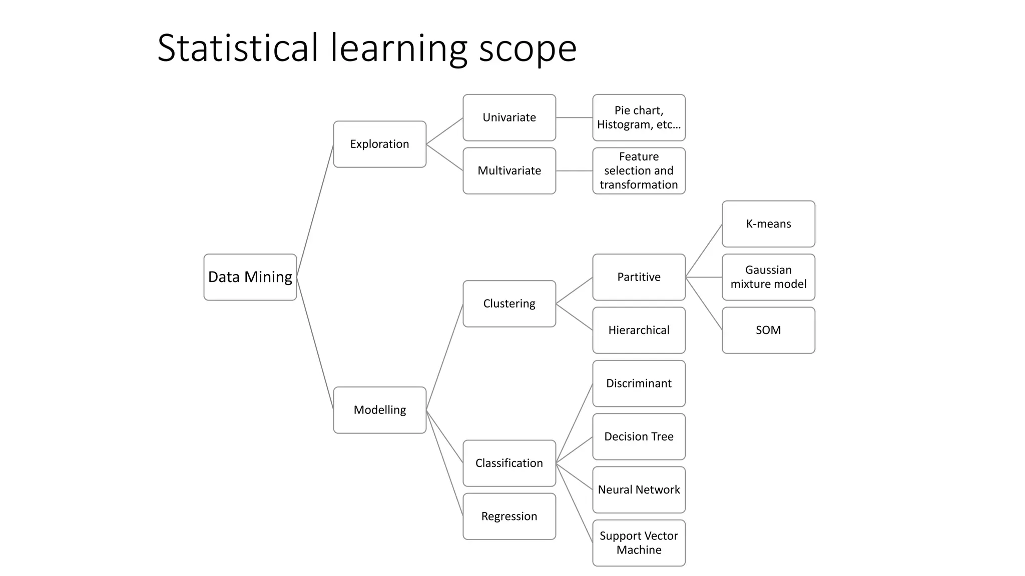
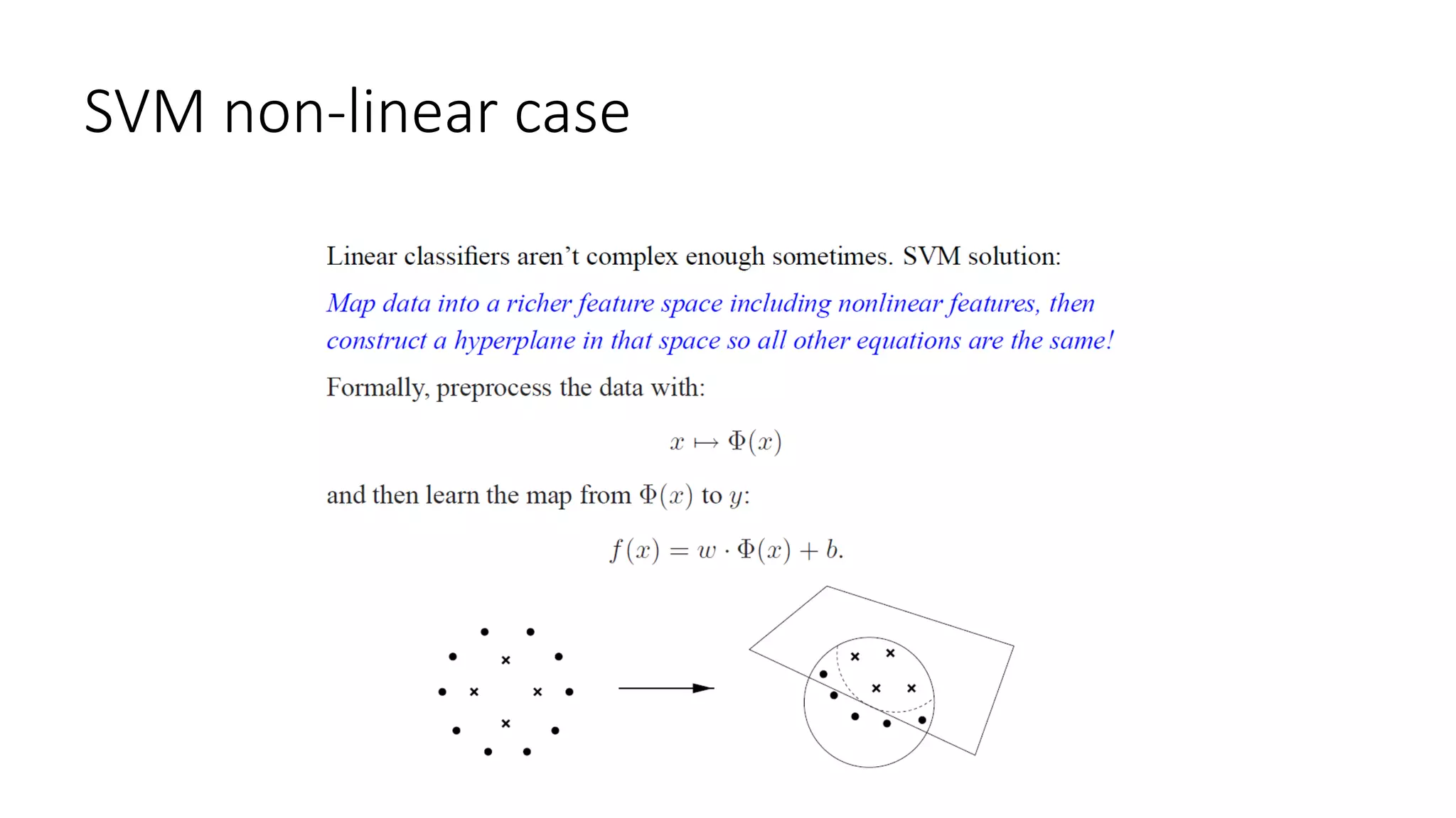
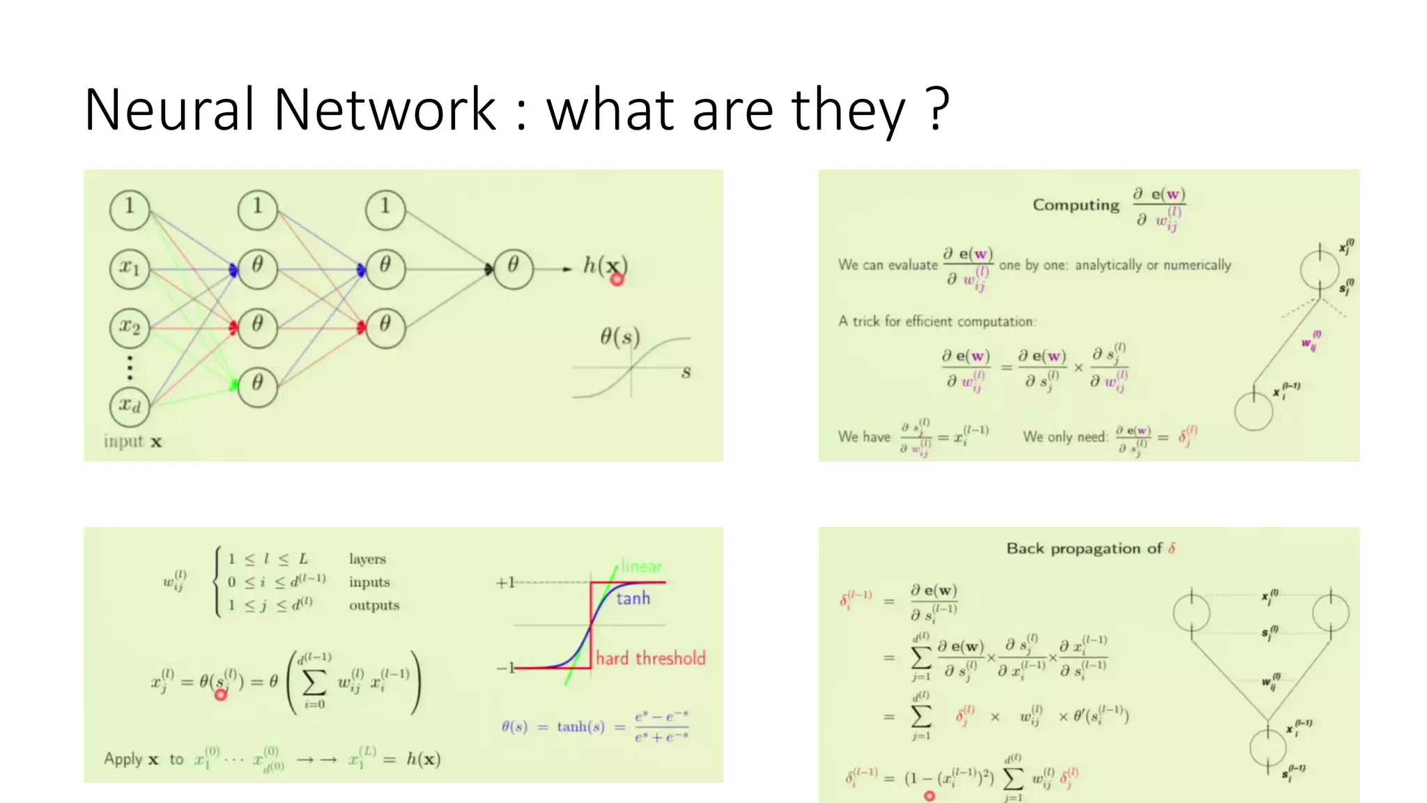
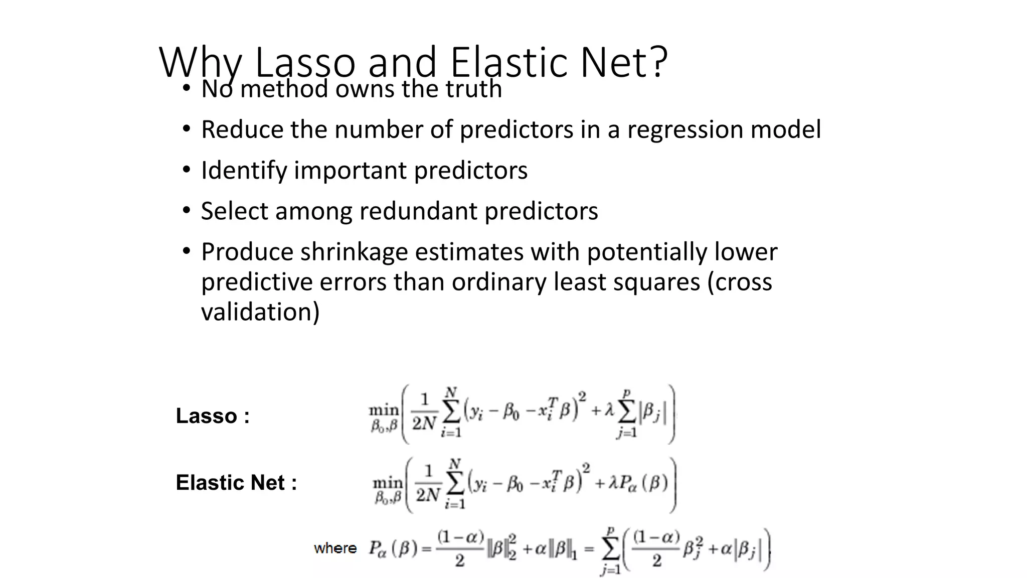
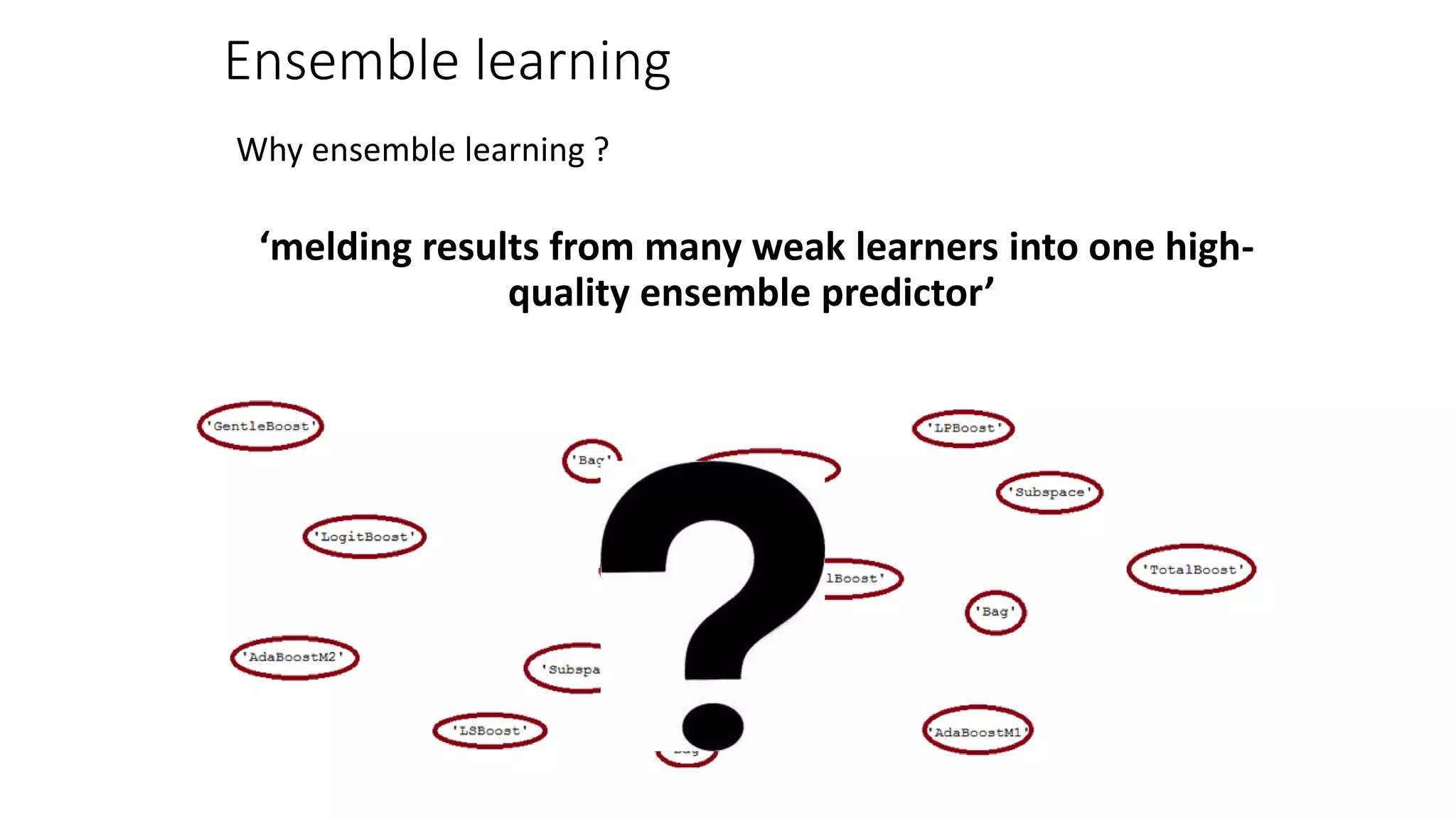
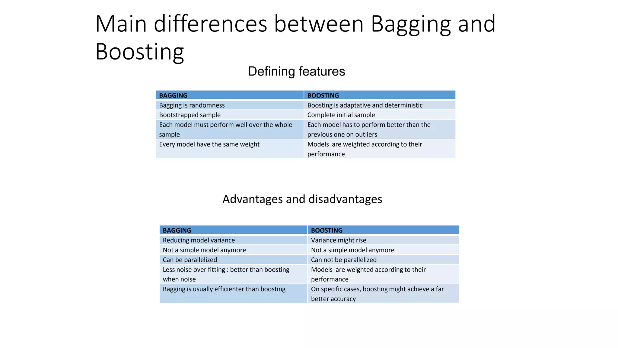
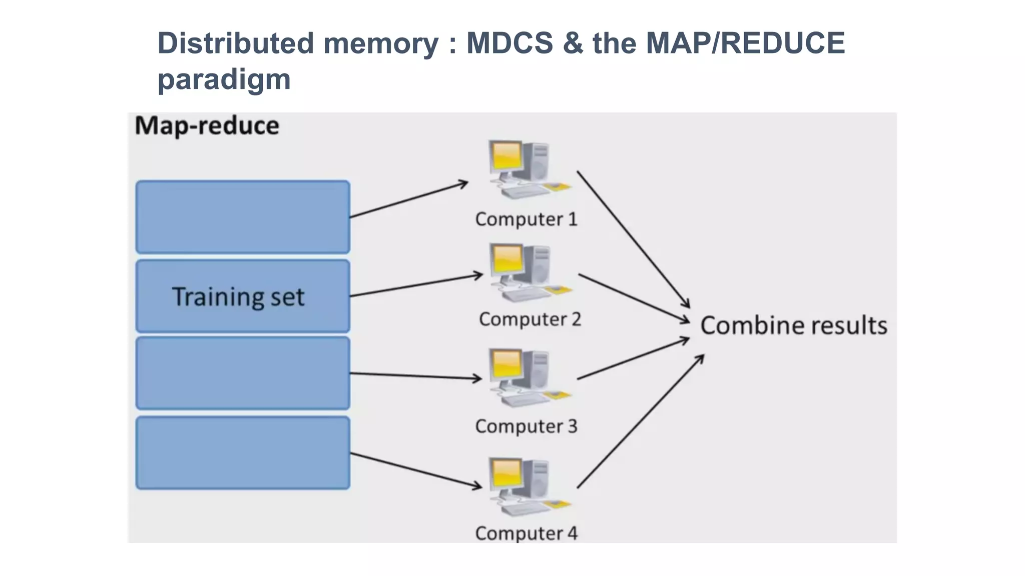
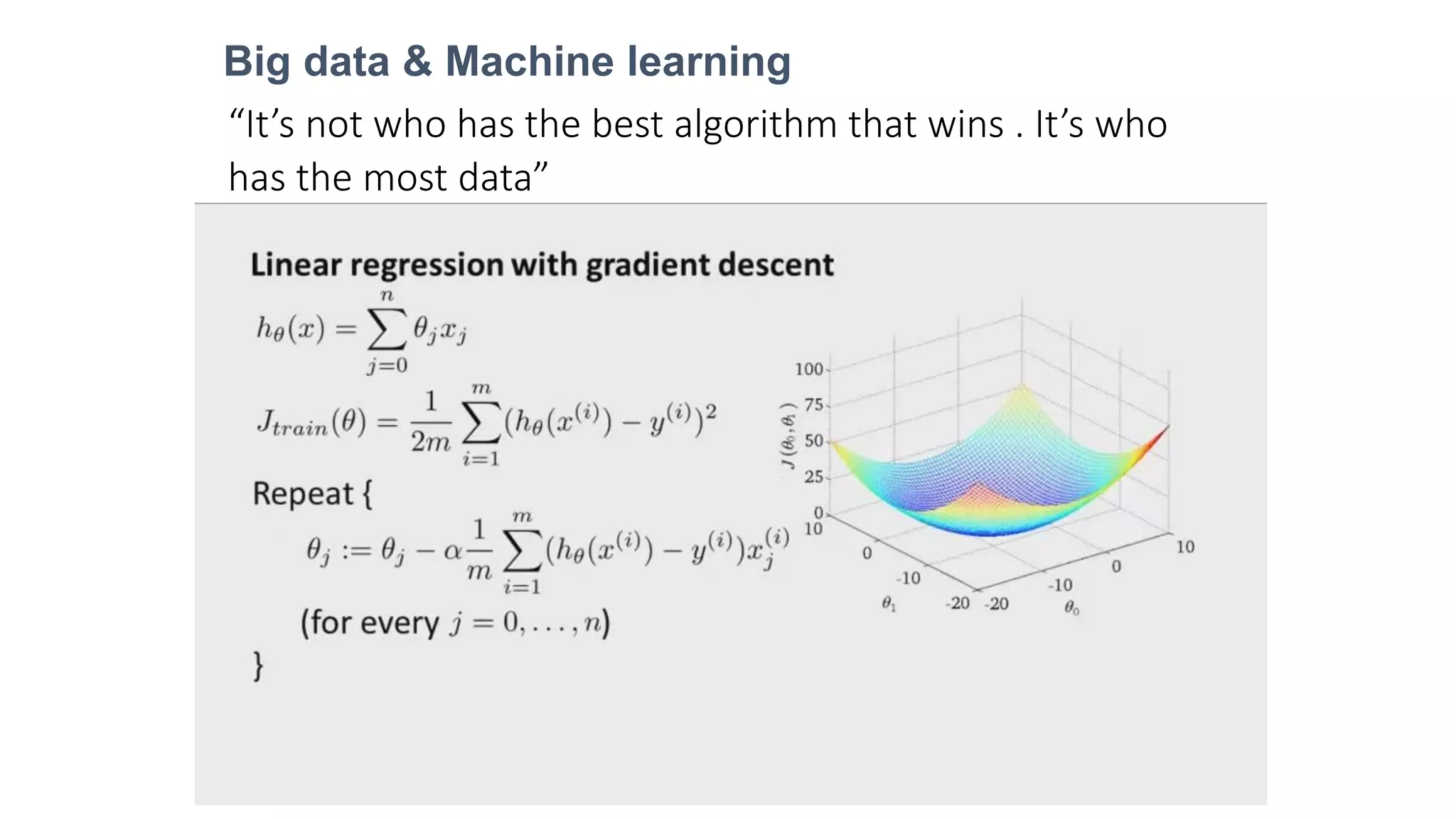
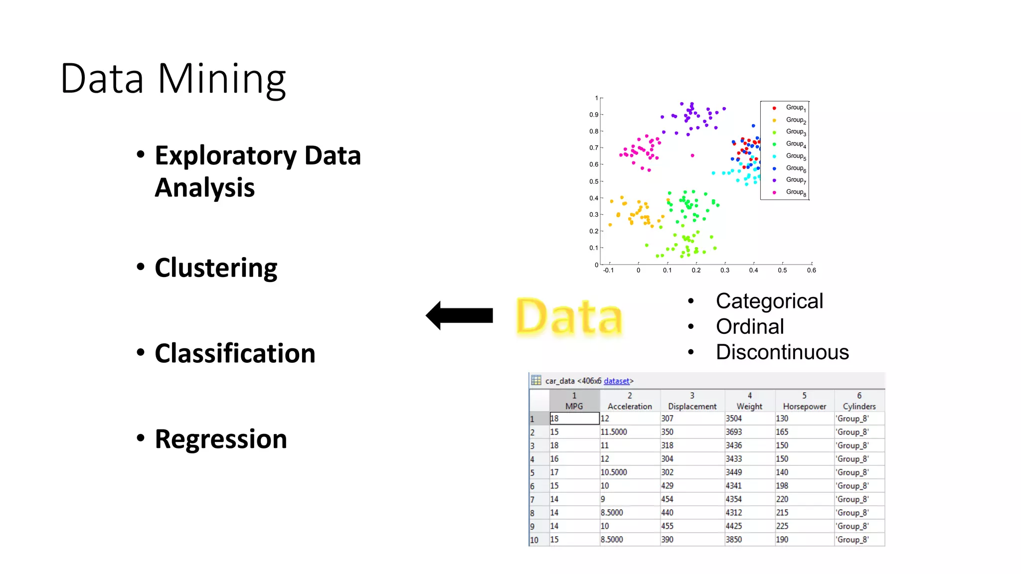
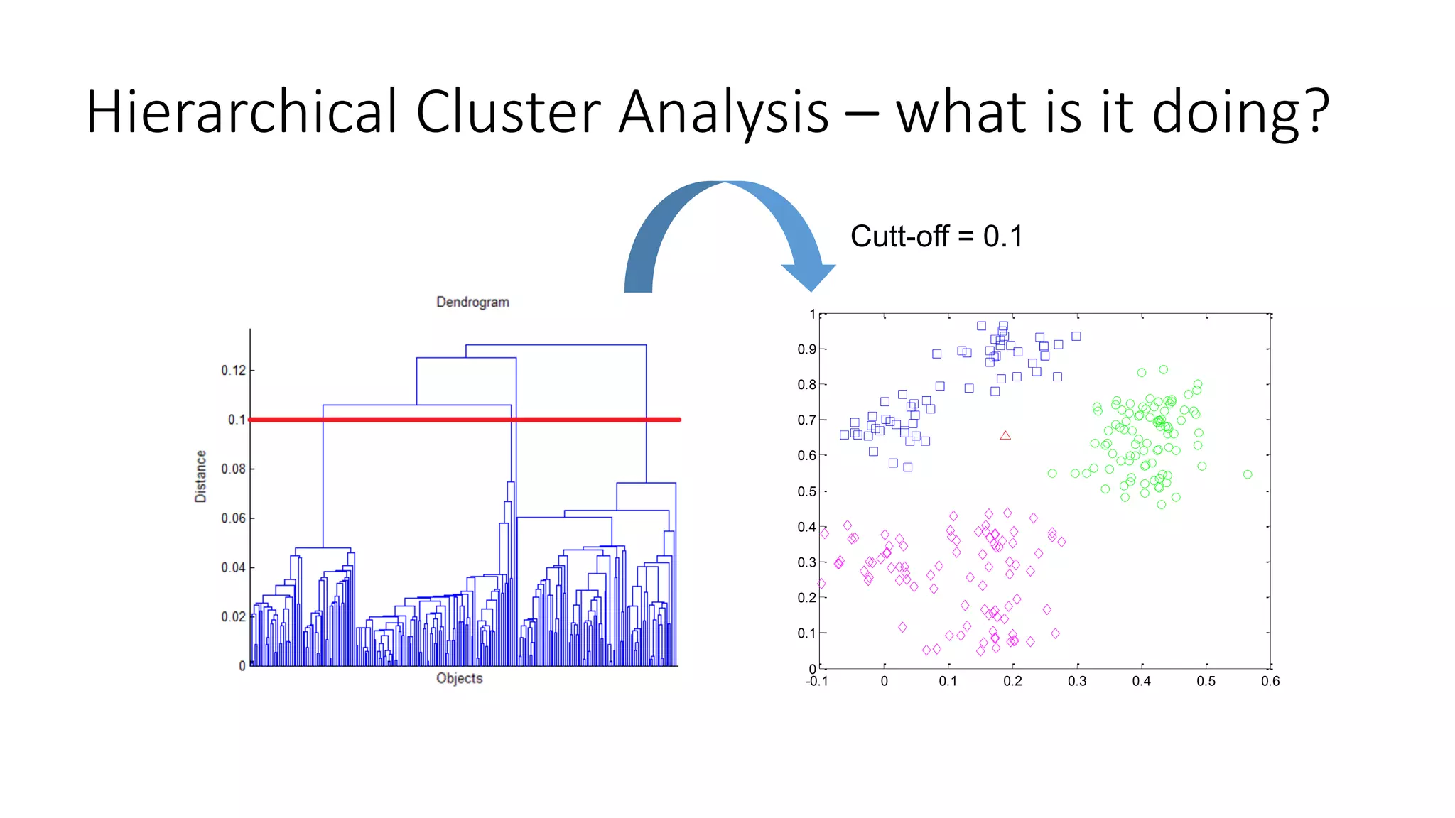
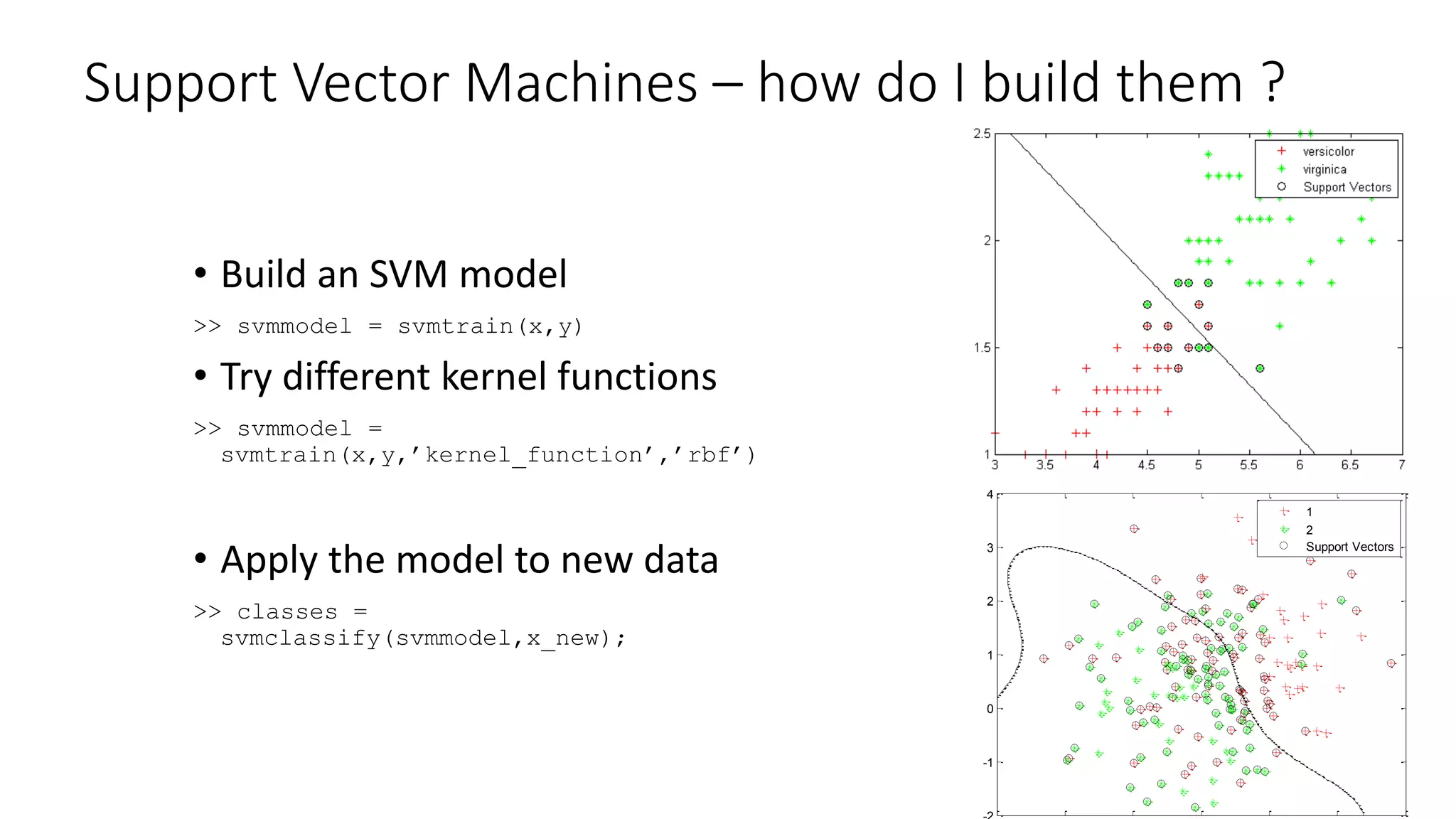
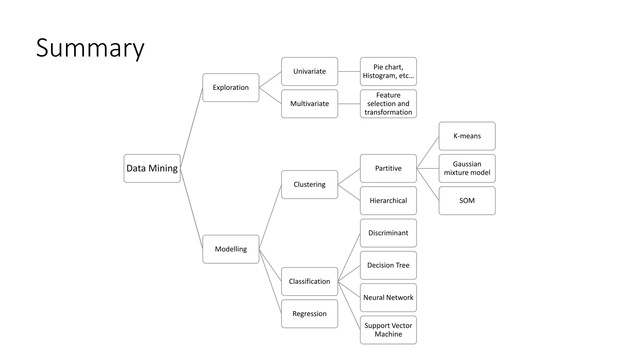
This document provides an overview of machine learning techniques that can be applied in finance, including exploratory data analysis, clustering, classification, and regression methods. It discusses statistical learning approaches like data mining and modeling. For clustering, it describes techniques like k-means clustering, hierarchical clustering, Gaussian mixture models, and self-organizing maps. For classification, it mentions discriminant analysis, decision trees, neural networks, and support vector machines. It also provides summaries of regression, ensemble methods, and working with big data and distributed learning.