HARNESSING R: STATISTICAL TECHNIQUES FOR DATA-DRIVEN ENTREPRENEURSHIP- Advanced Graphics with ggplot2, Introduction to Statistical Analysis��Types of Statistical Analysis, Descriptive Statistics�Inferential statistics, Probability Distributions in R�

![Basic R Commands
Arithmetic
Operations
x <- 10
y <- 3
x + y # Addition
x - y # Subtraction
x * y # Multiplication
x / y # Division
x ^ y # Power
Creating Vectors(c())
v <- c(2, 4, 6, 8, 10)
print(v)
Indexing and Subsetting
v[1] # First element
v[2:4] # Elements 2 to 4
v[v > 5] # Elements greater than 5](https://image.slidesharecdn.com/rsoftwareppt-251117152232-5c81c487/75/HARNESSING-R-STATISTICAL-TECHNIQUES-FOR-DATA-DRIVEN-ENTREPRENEURSHIP-13-2048.jpg)
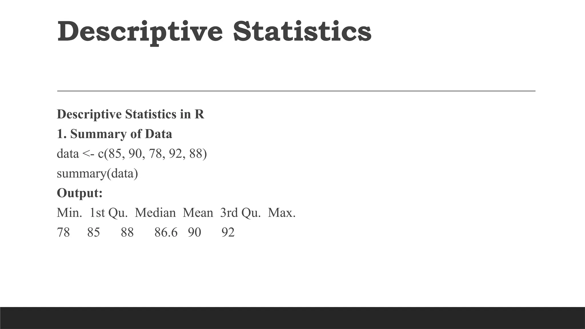
![Descriptive Statistics
2. Measures of Central Tendency
mean(data) # Mean
median(data) # Median
Output:
[1] 86.6
[1] 88](https://image.slidesharecdn.com/rsoftwareppt-251117152232-5c81c487/75/HARNESSING-R-STATISTICAL-TECHNIQUES-FOR-DATA-DRIVEN-ENTREPRENEURSHIP-23-2048.jpg)
![Descriptive Statistics
3. Measures of Spread (Dispersion)
var(data) # Variance
sd(data) # Standard Deviation
range(data) # Min & Max
Output:
[1] 34.3
[1] 5.86
[1] 78 92](https://image.slidesharecdn.com/rsoftwareppt-251117152232-5c81c487/75/HARNESSING-R-STATISTICAL-TECHNIQUES-FOR-DATA-DRIVEN-ENTREPRENEURSHIP-24-2048.jpg)
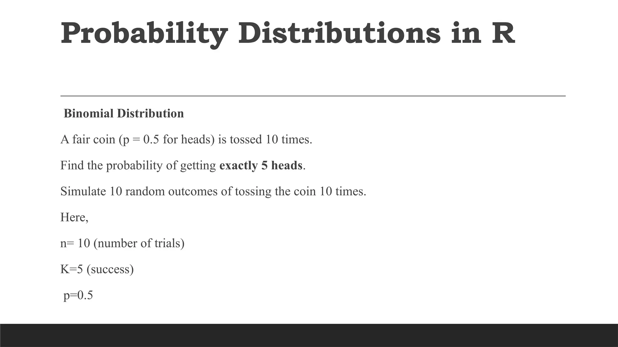
![# Probability of 5 successes in 10 trials with p=0.5
dbinom(5, size=10, prob=0.5)
# Generate random binomial values
rbinom(10, size=10, prob=0.5)
Output Example:
[1] 0.246 # Probability of exactly 5 successes
[1] 6 5 4 7 5 6 5 4 3 7 # Random outcomes
Probability Distributions in R](https://image.slidesharecdn.com/rsoftwareppt-251117152232-5c81c487/75/HARNESSING-R-STATISTICAL-TECHNIQUES-FOR-DATA-DRIVEN-ENTREPRENEURSHIP-38-2048.jpg)
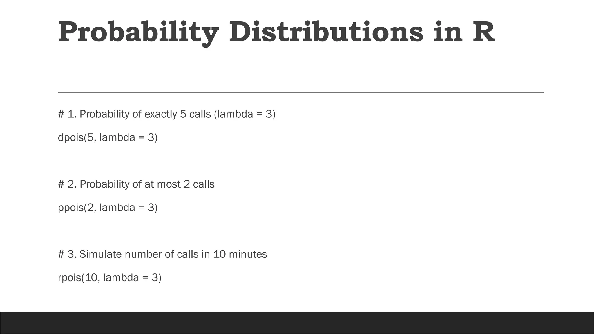
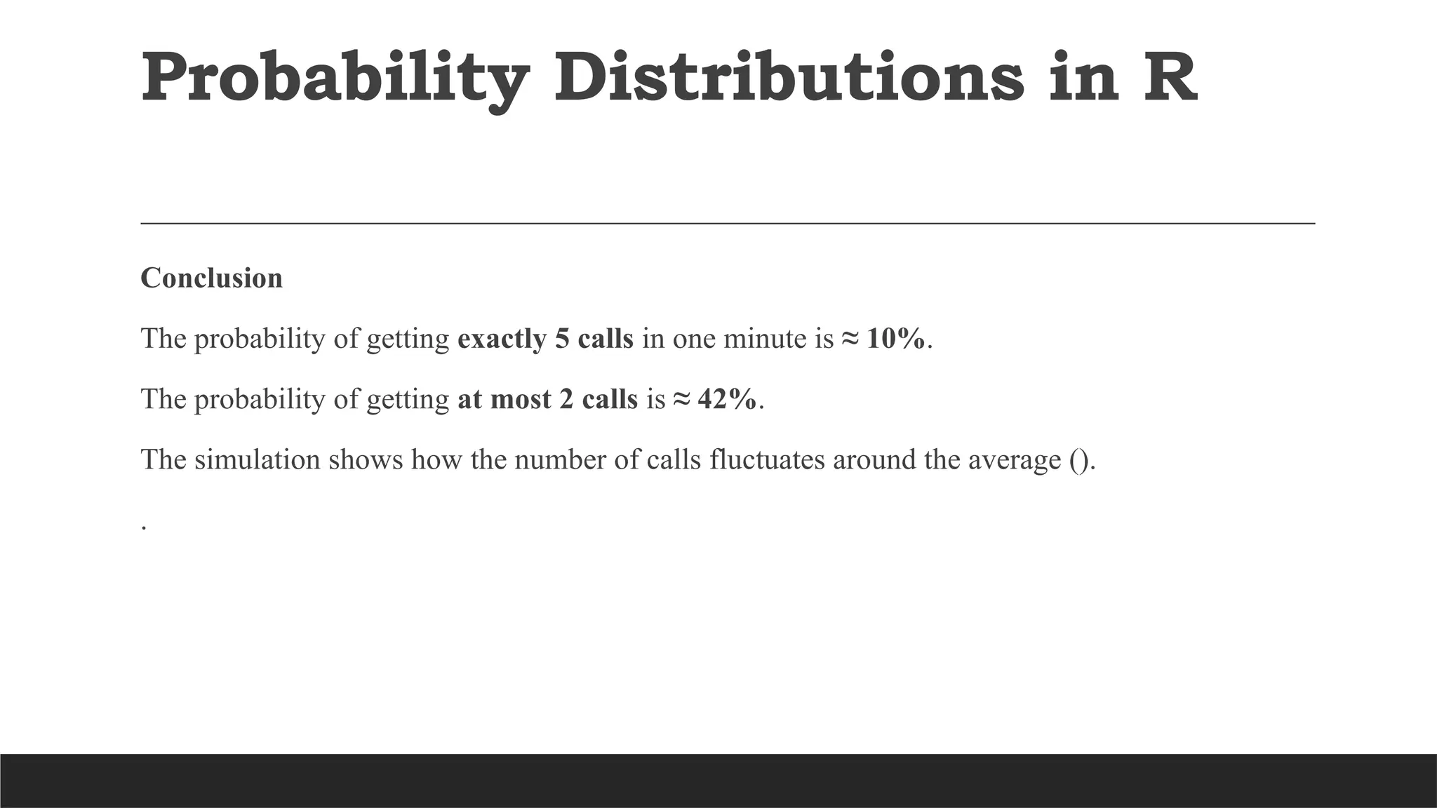
![# 1. Probability of exactly 5 calls
dpois(5, lambda = 3)
[1] 0.1008188
# 2. Probability of at most 2 calls
> ppois(2, lambda = 3)
[1] 0.4231901
# 3. Simulate number of calls in 10 minutes
rpois(10, lambda = 3)
[1] 3 3 1 4 2 2 3 2 0 8
Probability Distributions in R](https://image.slidesharecdn.com/rsoftwareppt-251117152232-5c81c487/75/HARNESSING-R-STATISTICAL-TECHNIQUES-FOR-DATA-DRIVEN-ENTREPRENEURSHIP-42-2048.jpg)
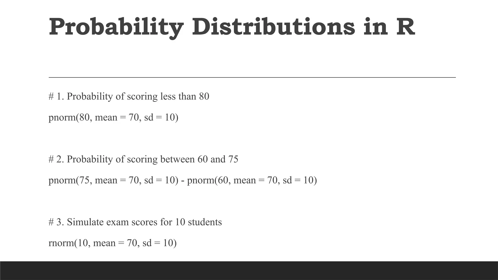
![P(X < 80):
pnorm(80, mean = 70, sd = 10)
# [1] 0.8413447
There is about 84.13% chance that a student scores less than 80.
P(60 < X < 75):
pnorm(75, mean = 70, sd = 10) - pnorm(60, mean = 70, sd = 10)
# [1] 0.5328072
There is about 53.28% chance that a student scores between 60 and 75.
Probability Distributions in R](https://image.slidesharecdn.com/rsoftwareppt-251117152232-5c81c487/75/HARNESSING-R-STATISTICAL-TECHNIQUES-FOR-DATA-DRIVEN-ENTREPRENEURSHIP-46-2048.jpg)
![Simulated scores:
rnorm(10, mean = 70, sd = 10)
# Example output: [1] 68.5 72.3 81.0 59.4 74.2 65.8 69.1 77.6 62.8 71.4
These are 10 randomly generated exam scores based on the normal distribution.
Conclusion
Most students are likely to score below 80 (84% probability).
Over half the students (53% probability) will fall between 60 and 75.
The simulated results reflect how scores cluster around the mean (70) with some variation due to
standard deviation.
Probability Distributions in R](https://image.slidesharecdn.com/rsoftwareppt-251117152232-5c81c487/75/HARNESSING-R-STATISTICAL-TECHNIQUES-FOR-DATA-DRIVEN-ENTREPRENEURSHIP-47-2048.jpg)


![Basic R Commands
Arithmetic
Operations
x <- 10
y <- 3
x + y # Addition
x - y # Subtraction
x * y # Multiplication
x / y # Division
x ^ y # Power
Creating Vectors(c())
v <- c(2, 4, 6, 8, 10)
print(v)
Indexing and Subsetting
v[1] # First element
v[2:4] # Elements 2 to 4
v[v > 5] # Elements greater than 5](https://crownmelresort.com/image.slidesharecdn.com/rsoftwareppt-251117152232-5c81c487/75/HARNESSING-R-STATISTICAL-TECHNIQUES-FOR-DATA-DRIVEN-ENTREPRENEURSHIP-13-2048.jpg)


![Descriptive Statistics
2. Measures of Central Tendency
mean(data) # Mean
median(data) # Median
Output:
[1] 86.6
[1] 88](https://crownmelresort.com/image.slidesharecdn.com/rsoftwareppt-251117152232-5c81c487/75/HARNESSING-R-STATISTICAL-TECHNIQUES-FOR-DATA-DRIVEN-ENTREPRENEURSHIP-23-2048.jpg)
![Descriptive Statistics
3. Measures of Spread (Dispersion)
var(data) # Variance
sd(data) # Standard Deviation
range(data) # Min & Max
Output:
[1] 34.3
[1] 5.86
[1] 78 92](https://crownmelresort.com/image.slidesharecdn.com/rsoftwareppt-251117152232-5c81c487/75/HARNESSING-R-STATISTICAL-TECHNIQUES-FOR-DATA-DRIVEN-ENTREPRENEURSHIP-24-2048.jpg)


![# Probability of 5 successes in 10 trials with p=0.5
dbinom(5, size=10, prob=0.5)
# Generate random binomial values
rbinom(10, size=10, prob=0.5)
Output Example:
[1] 0.246 # Probability of exactly 5 successes
[1] 6 5 4 7 5 6 5 4 3 7 # Random outcomes
Probability Distributions in R](https://crownmelresort.com/image.slidesharecdn.com/rsoftwareppt-251117152232-5c81c487/75/HARNESSING-R-STATISTICAL-TECHNIQUES-FOR-DATA-DRIVEN-ENTREPRENEURSHIP-38-2048.jpg)


![# 1. Probability of exactly 5 calls
dpois(5, lambda = 3)
[1] 0.1008188
# 2. Probability of at most 2 calls
> ppois(2, lambda = 3)
[1] 0.4231901
# 3. Simulate number of calls in 10 minutes
rpois(10, lambda = 3)
[1] 3 3 1 4 2 2 3 2 0 8
Probability Distributions in R](https://crownmelresort.com/image.slidesharecdn.com/rsoftwareppt-251117152232-5c81c487/75/HARNESSING-R-STATISTICAL-TECHNIQUES-FOR-DATA-DRIVEN-ENTREPRENEURSHIP-42-2048.jpg)


![P(X < 80):
pnorm(80, mean = 70, sd = 10)
# [1] 0.8413447
There is about 84.13% chance that a student scores less than 80.
P(60 < X < 75):
pnorm(75, mean = 70, sd = 10) - pnorm(60, mean = 70, sd = 10)
# [1] 0.5328072
There is about 53.28% chance that a student scores between 60 and 75.
Probability Distributions in R](https://crownmelresort.com/image.slidesharecdn.com/rsoftwareppt-251117152232-5c81c487/75/HARNESSING-R-STATISTICAL-TECHNIQUES-FOR-DATA-DRIVEN-ENTREPRENEURSHIP-46-2048.jpg)
![Simulated scores:
rnorm(10, mean = 70, sd = 10)
# Example output: [1] 68.5 72.3 81.0 59.4 74.2 65.8 69.1 77.6 62.8 71.4
These are 10 randomly generated exam scores based on the normal distribution.
Conclusion
Most students are likely to score below 80 (84% probability).
Over half the students (53% probability) will fall between 60 and 75.
The simulated results reflect how scores cluster around the mean (70) with some variation due to
standard deviation.
Probability Distributions in R](https://crownmelresort.com/image.slidesharecdn.com/rsoftwareppt-251117152232-5c81c487/75/HARNESSING-R-STATISTICAL-TECHNIQUES-FOR-DATA-DRIVEN-ENTREPRENEURSHIP-47-2048.jpg)


![Basics of R programming for analytics [Autosaved] (1).pdf](https://cdn.slidesharecdn.com/ss_thumbnails/basicsofrprogrammingforanalyticsautosaved1-240916080545-0682f8c8-thumbnail.jpg?width=640&height=640&fit=bounds)


![[Redis Released]- FalkorDB - Redis + Graph Agentic Memory’s Secret Sauce](https://cdn.slidesharecdn.com/ss_thumbnails/redisreleased-falkordbslidedeck-1125-251115194922-e1c0046b-thumbnail.jpg?width=640&height=640&fit=bounds)


