Populations and Samplesin Statistical
Analysis
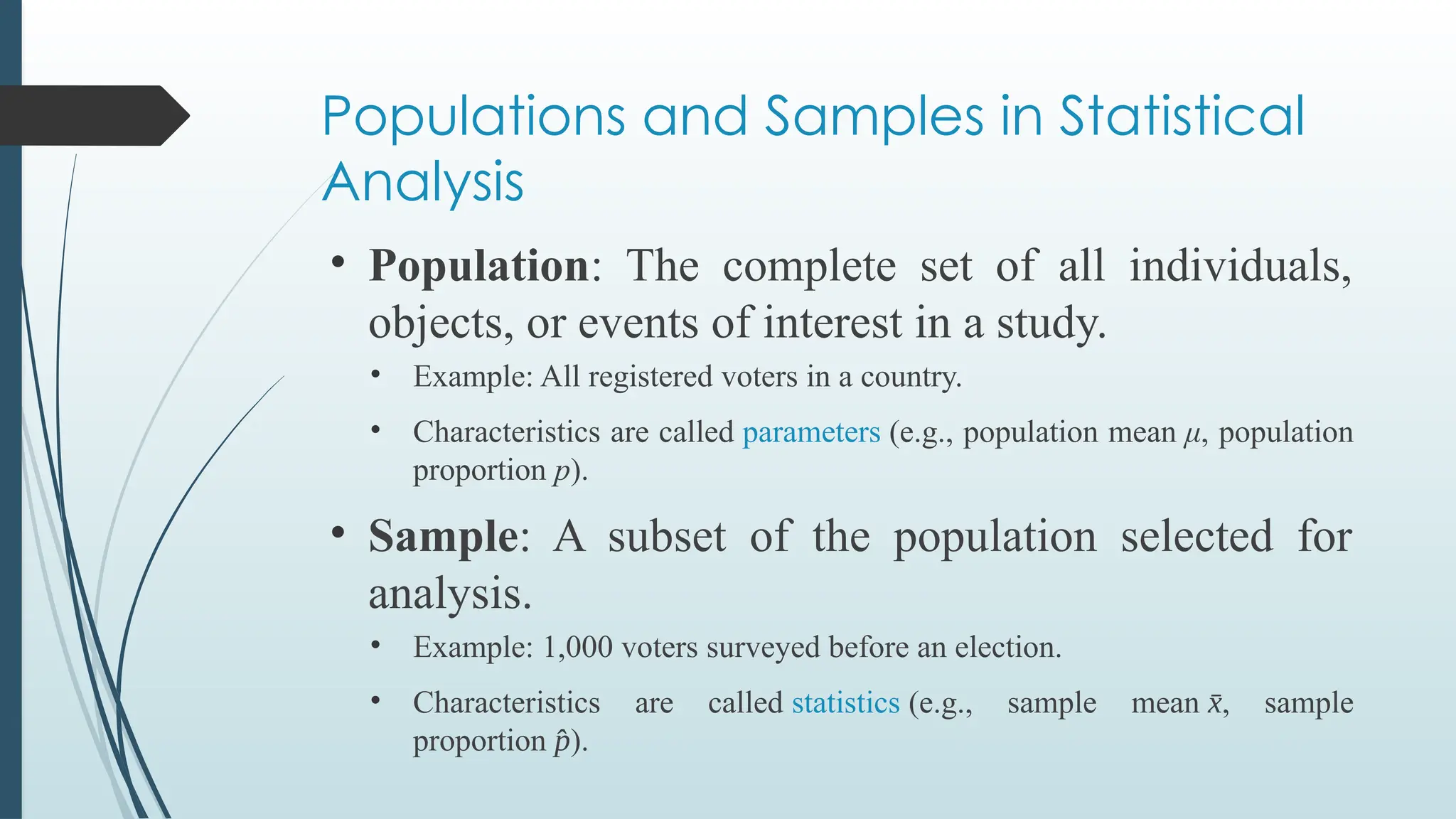
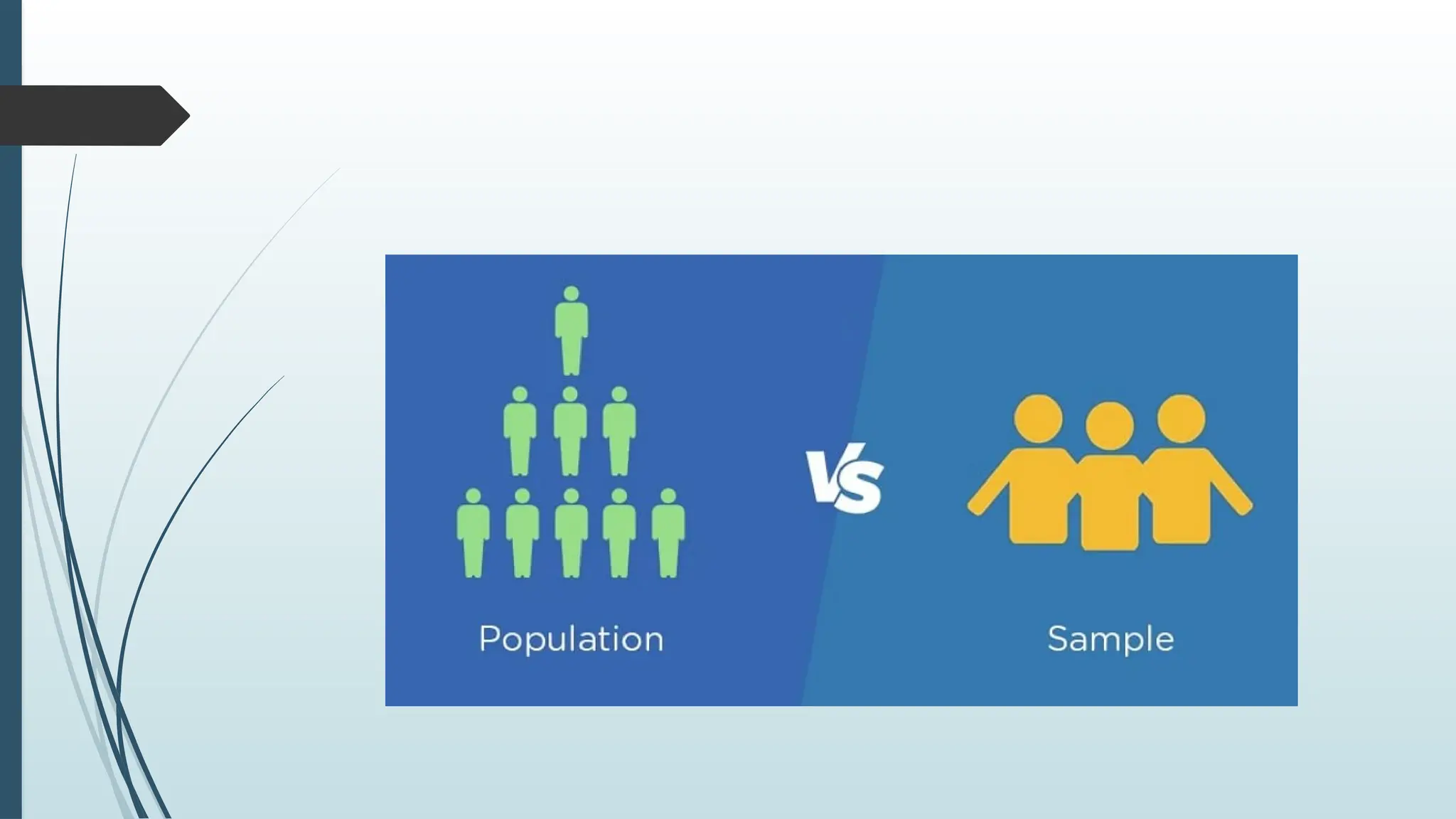
• Population: The complete set of all individuals,
objects, or events of interest in a study.
• Example: All registered voters in a country.
• Characteristics are called parameters (e.g., population mean μ, population
proportion p).
• Sample: A subset of the population selected for
analysis.
• Example: 1,000 voters surveyed before an election.
• Characteristics are called statistics (e.g., sample mean x
̄ , sample
proportion p
̂ ).
4.
Why Use SamplesInstead of Populations?
Cost & Practicality: Measuring an entire population is often
expensive or impossible.
Time Efficiency: Sampling allows faster data collection and
analysis.
Feasibility: Some tests are destructive (e.g., crash-testing cars).
Accuracy: Proper sampling can yield highly precise estimates.
Probability Sampling
• SimpleRandom Sampling: Every member has an equal chance of
selection.
• Stratified Sampling: Population divided into subgroups (strata),
then random samples are taken from each.
• Cluster Sampling: Population divided into clusters (e.g., cities),
and entire clusters are randomly selected.
• Systematic Sampling: Selecting every k-th element from a list
(e.g., every 10th person).
7.
Non-Probability Sampling
• ConvenienceSampling: Using readily available subjects (e.g.,
online surveys).
• Purposive Sampling: Selecting subjects based on researcher’s
judgment.
• Snowball Sampling: Existing participants recruit others (used in
hard-to-reach populations).
8.
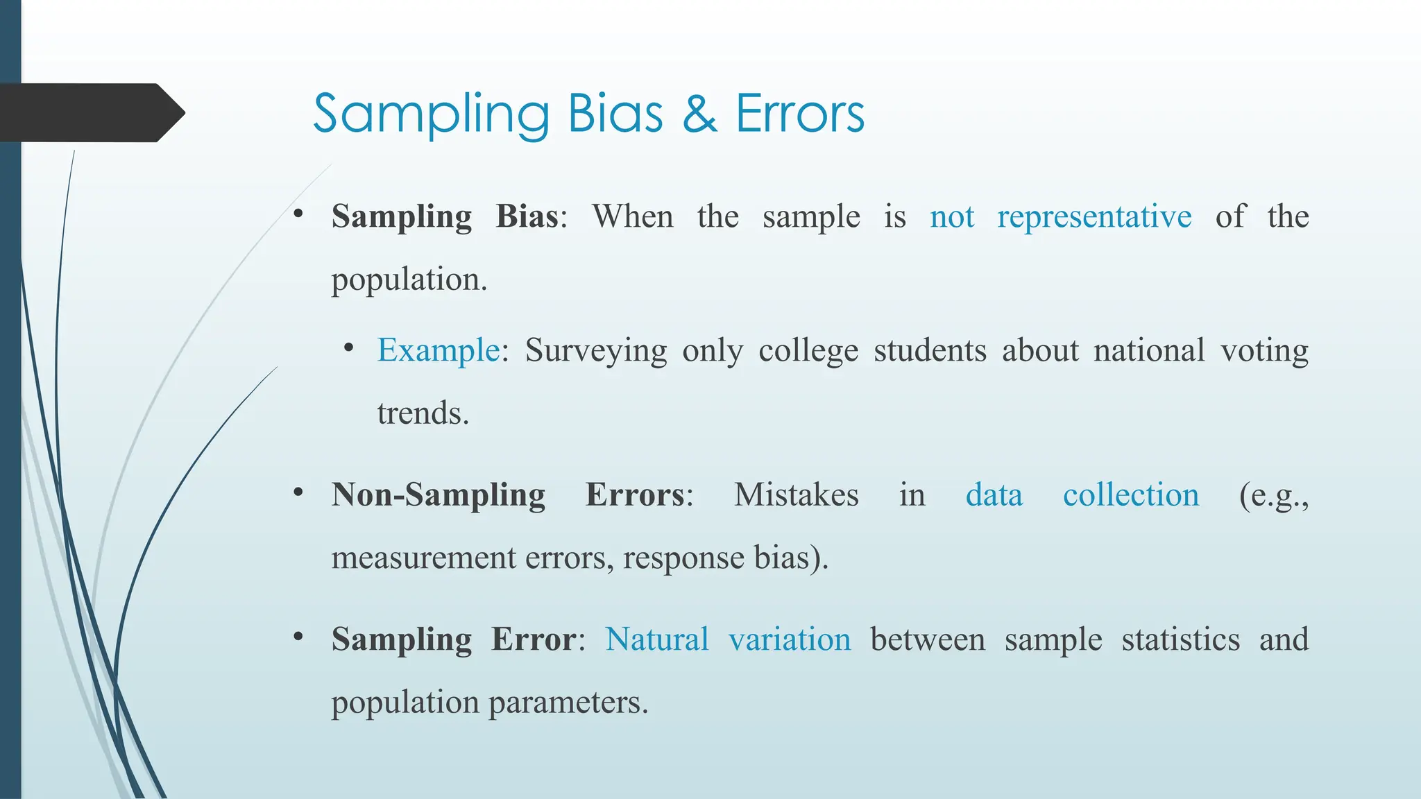
Sampling Bias &Errors
• Sampling Bias: When the sample is not representative of the
population.
• Example: Surveying only college students about national voting
trends.
• Non-Sampling Errors: Mistakes in data collection (e.g.,
measurement errors, response bias).
• Sampling Error: Natural variation between sample statistics and
population parameters.
9.
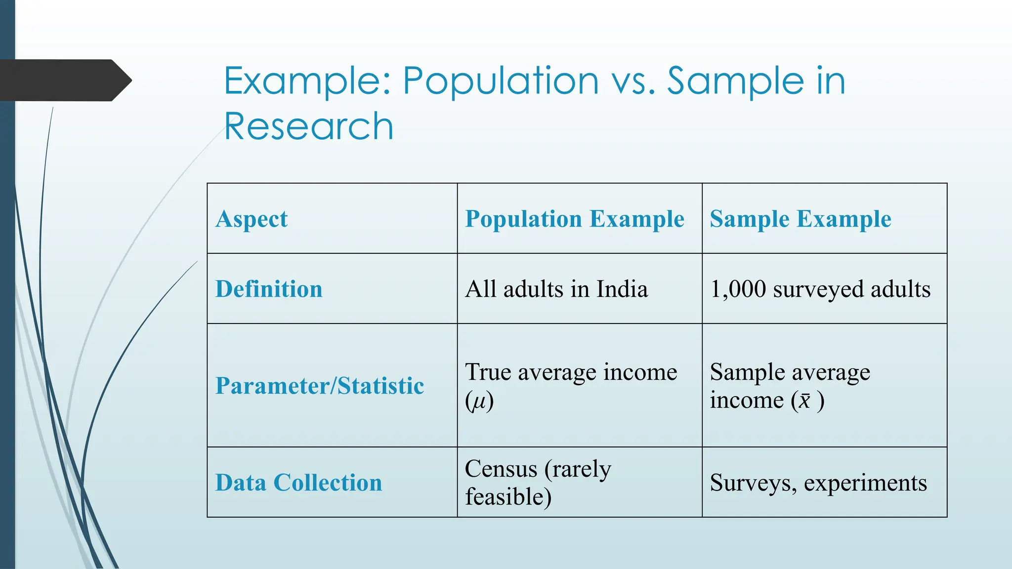
Example: Population vs.Sample in
Research
Aspect Population Example Sample Example
Definition All adults in India 1,000 surveyed adults
Parameter/Statistic
True average income
(μ)
Sample average
income (x
̄ )
Data Collection
Census (rarely
feasible)
Surveys, experiments
10.
Statistical Modelling
Statistical modellinginvolves using mathematical equations to
represent relationships in data. Models help:
• Describe patterns in observed data
• Predict future outcomes
• Infer causal relationships
Statistical models can be broadly categorized into descriptive,
predictive, prescriptive, and inferential models, each serving a unique
purpose, from summarizing data to making predictions and
recommendations.
11.
1. Descriptive Models:
Purpose:Summarize and describe the characteristics of a dataset.
Examples:
Descriptive Statistics: Calculating measures like mean, median,
mode, standard deviation, and percentiles.
Frequency Distributions and Histograms: Visualizing the
distribution of data.
Scatterplots and Line Graphs: Showing relationships between
variables.
12.
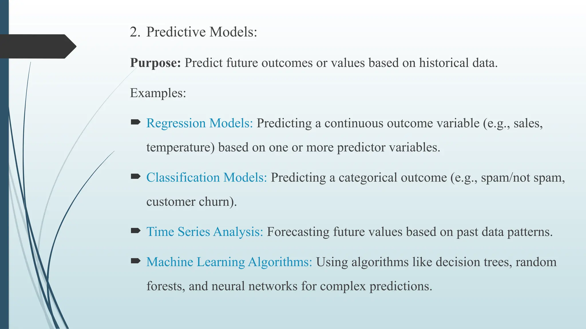
2. Predictive Models:
Purpose:Predict future outcomes or values based on historical data.
Examples:
Regression Models: Predicting a continuous outcome variable (e.g., sales,
temperature) based on one or more predictor variables.
Classification Models: Predicting a categorical outcome (e.g., spam/not spam,
customer churn).
Time Series Analysis: Forecasting future values based on past data patterns.
Machine Learning Algorithms: Using algorithms like decision trees, random
forests, and neural networks for complex predictions.
13.
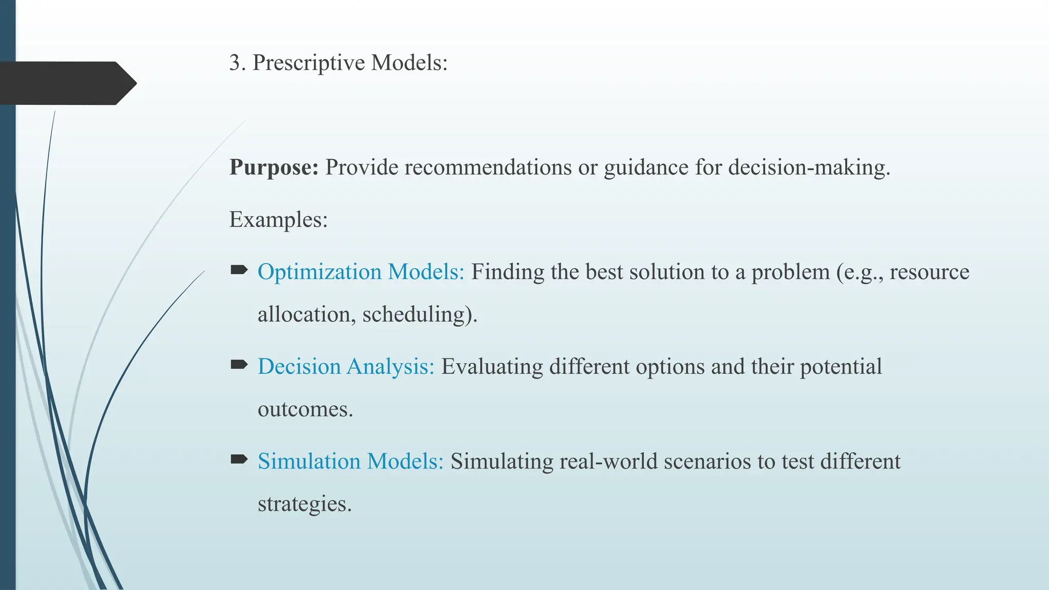
3. Prescriptive Models:
Purpose:Provide recommendations or guidance for decision-making.
Examples:
Optimization Models: Finding the best solution to a problem (e.g., resource
allocation, scheduling).
Decision Analysis: Evaluating different options and their potential
outcomes.
Simulation Models: Simulating real-world scenarios to test different
strategies.
14.
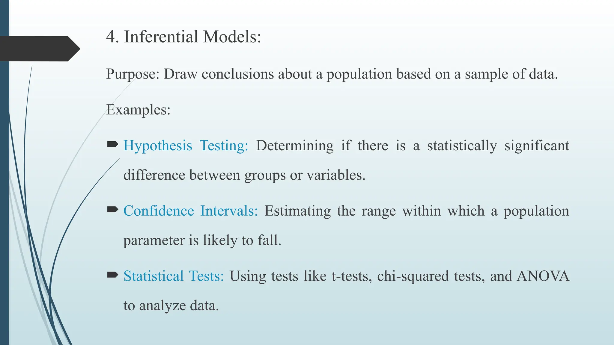
4. Inferential Models:
Purpose:Draw conclusions about a population based on a sample of data.
Examples:
Hypothesis Testing: Determining if there is a statistically significant
difference between groups or variables.
Confidence Intervals: Estimating the range within which a population
parameter is likely to fall.
Statistical Tests: Using tests like t-tests, chi-squared tests, and ANOVA
to analyze data.
15.
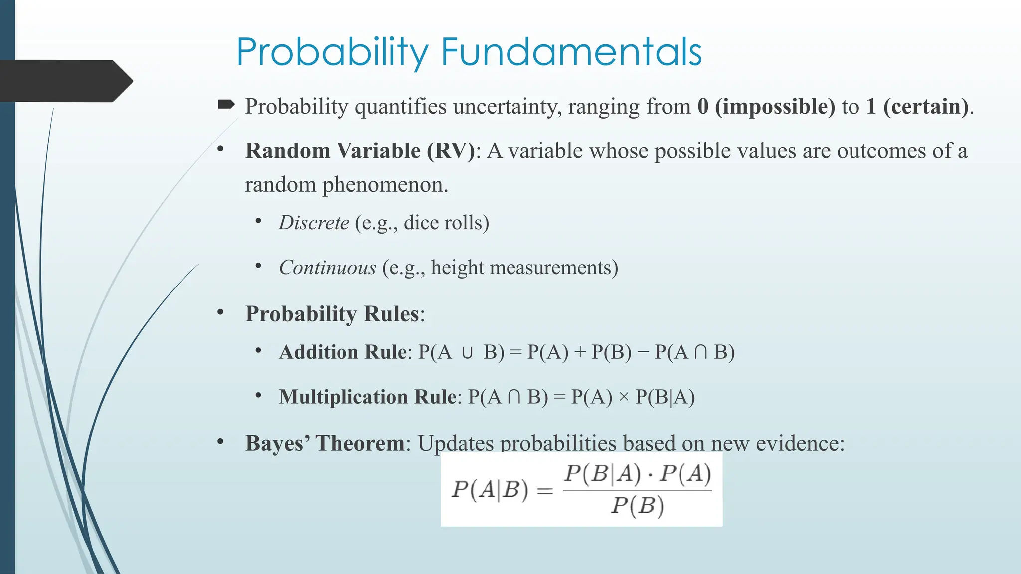
Probability Fundamentals
Probabilityquantifies uncertainty, ranging from 0 (impossible) to 1 (certain).
• Random Variable (RV): A variable whose possible values are outcomes of a
random phenomenon.
• Discrete (e.g., dice rolls)
• Continuous (e.g., height measurements)
• Probability Rules:
• Addition Rule: P(A B) = P(A) + P(B) − P(A ∩ B)
∪
• Multiplication Rule: P(A ∩ B) = P(A) × P(B|A)
• Bayes’ Theorem: Updates probabilities based on new evidence:
16.
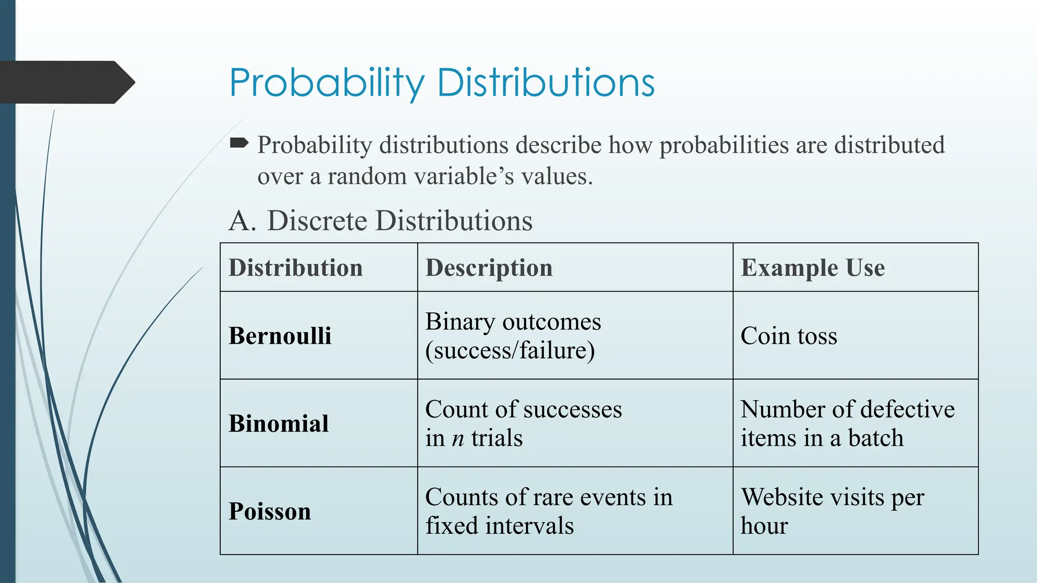
Probability Distributions
Probabilitydistributions describe how probabilities are distributed
over a random variable’s values.
A. Discrete Distributions
Distribution Description Example Use
Bernoulli
Binary outcomes
(success/failure)
Coin toss
Binomial
Count of successes
in n trials
Number of defective
items in a batch
Poisson
Counts of rare events in
fixed intervals
Website visits per
hour
17.
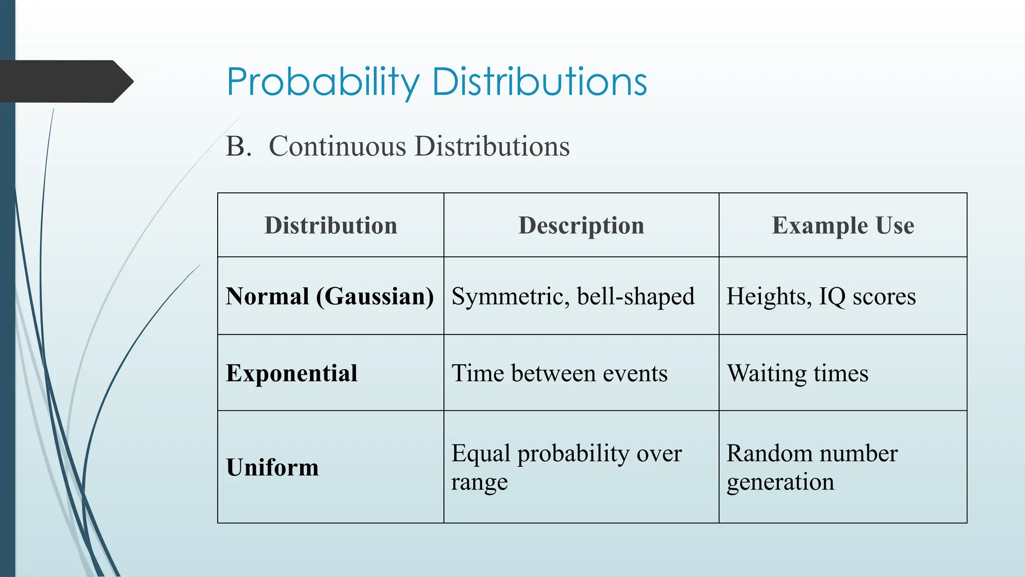
Probability Distributions
B. ContinuousDistributions
Distribution Description Example Use
Normal (Gaussian) Symmetric, bell-shaped Heights, IQ scores
Exponential Time between events Waiting times
Uniform
Equal probability over
range
Random number
generation
18.
Getting started withR
1. Redirect to https://cloud.r-project.org/
2. Download and install R
19.
What is R?
R is a popular programming language used for statistical computing
and graphical presentation.
Its most common use is to analyze and visualize data.
20.
Why Use R?
It is a great resource for data analysis, data visualization, data
science and machine learning
It provides many statistical techniques (such as statistical tests,
classification, clustering and data reduction)
It is easy to draw graphs in R, like pie charts, histograms, box plot,
scatter plot, etc++
It works on different platforms (Windows, Mac, Linux)
It is open-source and free
It has a large community support
It has many packages (libraries of functions) that can be used to
solve different problems
21.
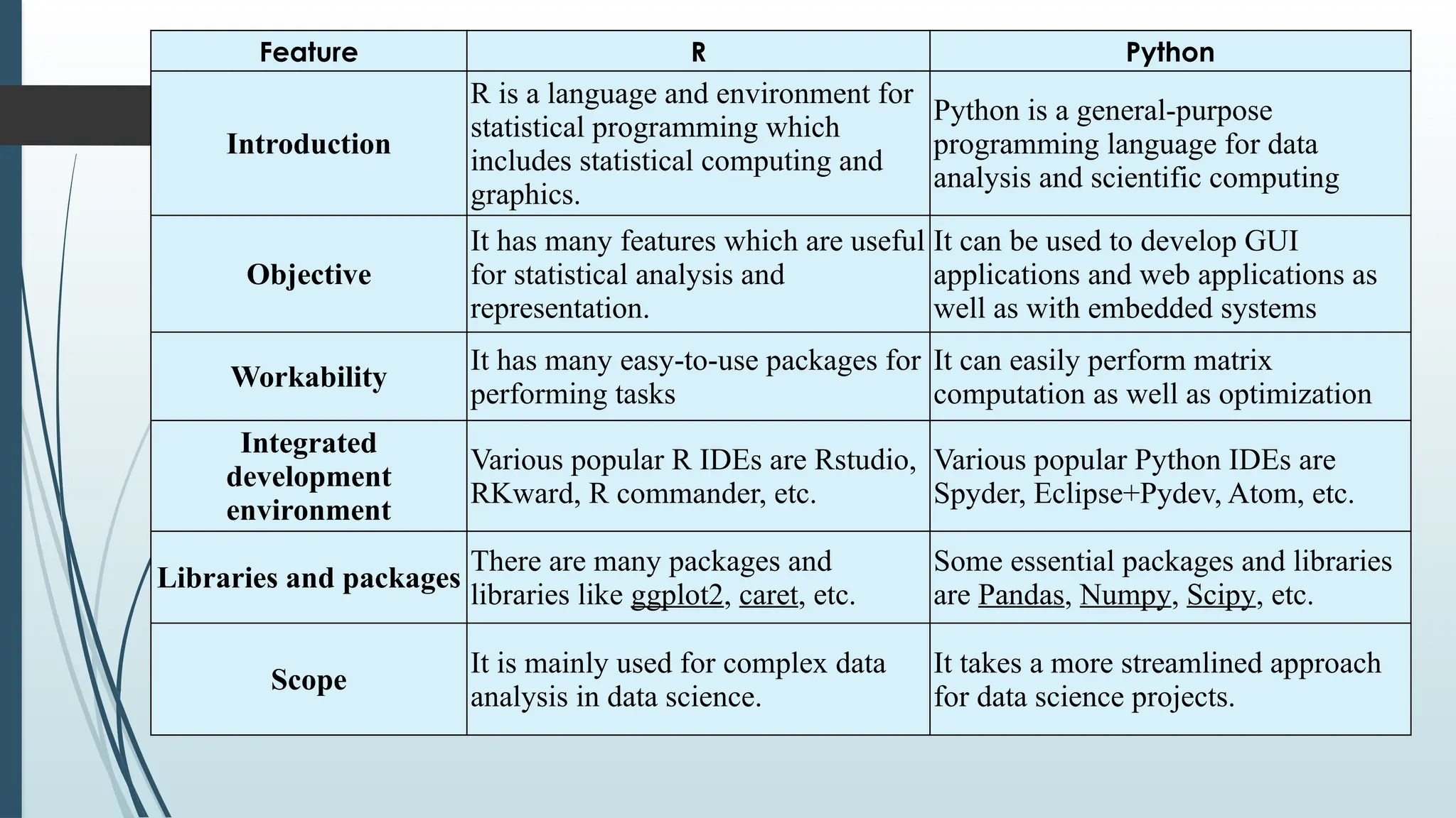
Feature R Python
Introduction
Ris a language and environment for
statistical programming which
includes statistical computing and
graphics.
Python is a general-purpose
programming language for data
analysis and scientific computing
Objective
It has many features which are useful
for statistical analysis and
representation.
It can be used to develop GUI
applications and web applications as
well as with embedded systems
Workability
It has many easy-to-use packages for
performing tasks
It can easily perform matrix
computation as well as optimization
Integrated
development
environment
Various popular R IDEs are Rstudio,
RKward, R commander, etc.
Various popular Python IDEs are
Spyder, Eclipse+Pydev, Atom, etc.
Libraries and packages
There are many packages and
libraries like ggplot2, caret, etc.
Some essential packages and libraries
are Pandas, Numpy, Scipy, etc.
Scope
It is mainly used for complex data
analysis in data science.
It takes a more streamlined approach
for data science projects.
22.
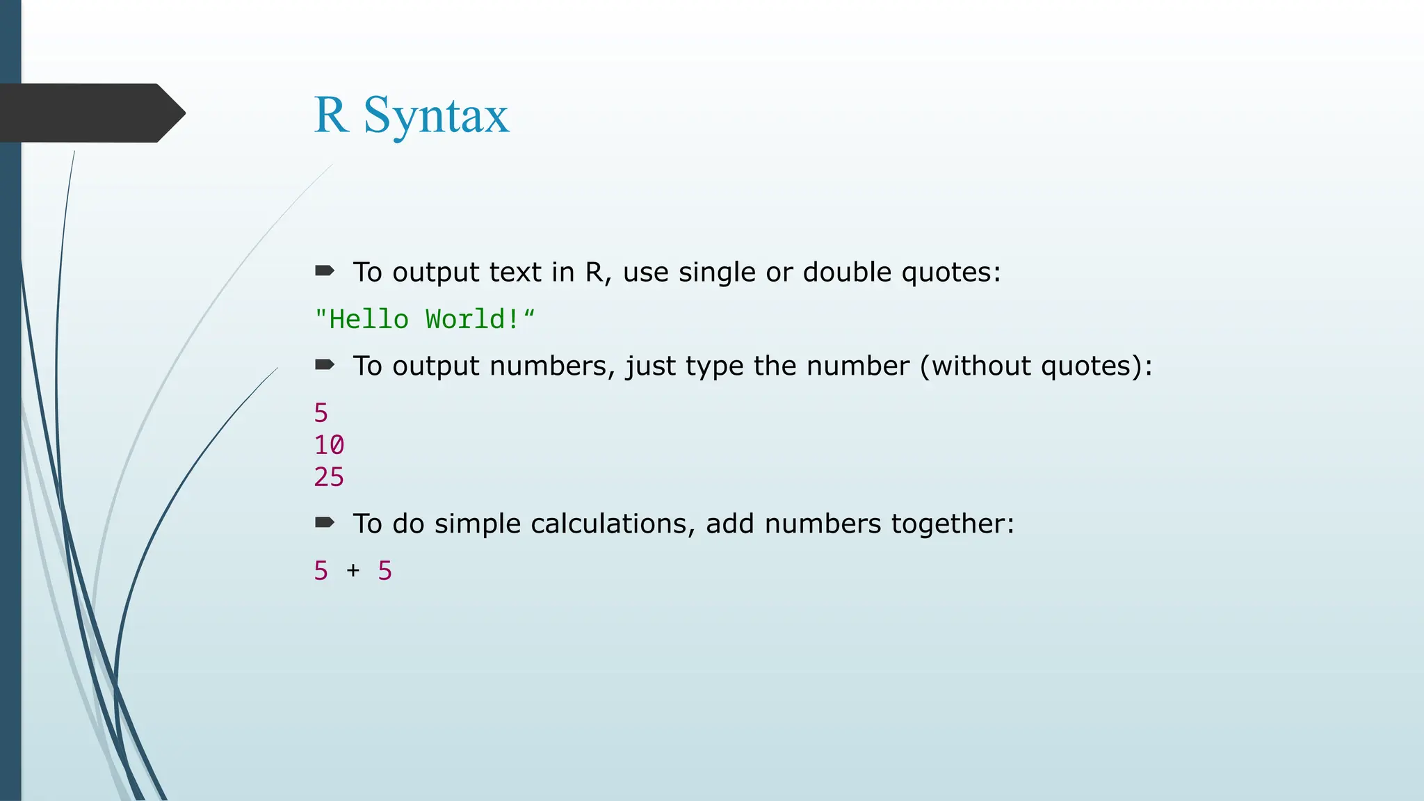
R Syntax
Tooutput text in R, use single or double quotes:
"Hello World!“
To output numbers, just type the number (without quotes):
5
10
25
To do simple calculations, add numbers together:
5 + 5
23.
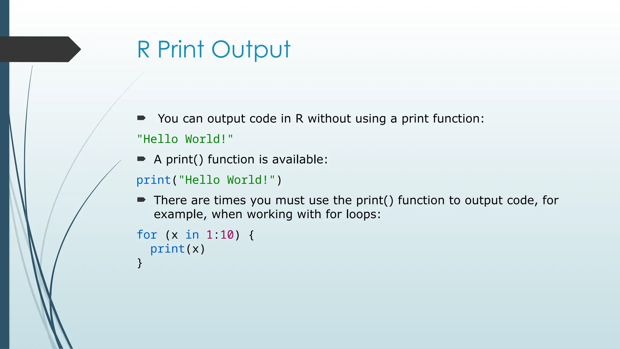
R Print Output
You can output code in R without using a print function:
"Hello World!"
A print() function is available:
print("Hello World!")
There are times you must use the print() function to output code, for
example, when working with for loops:
for (x in 1:10) {
print(x)
}
24.
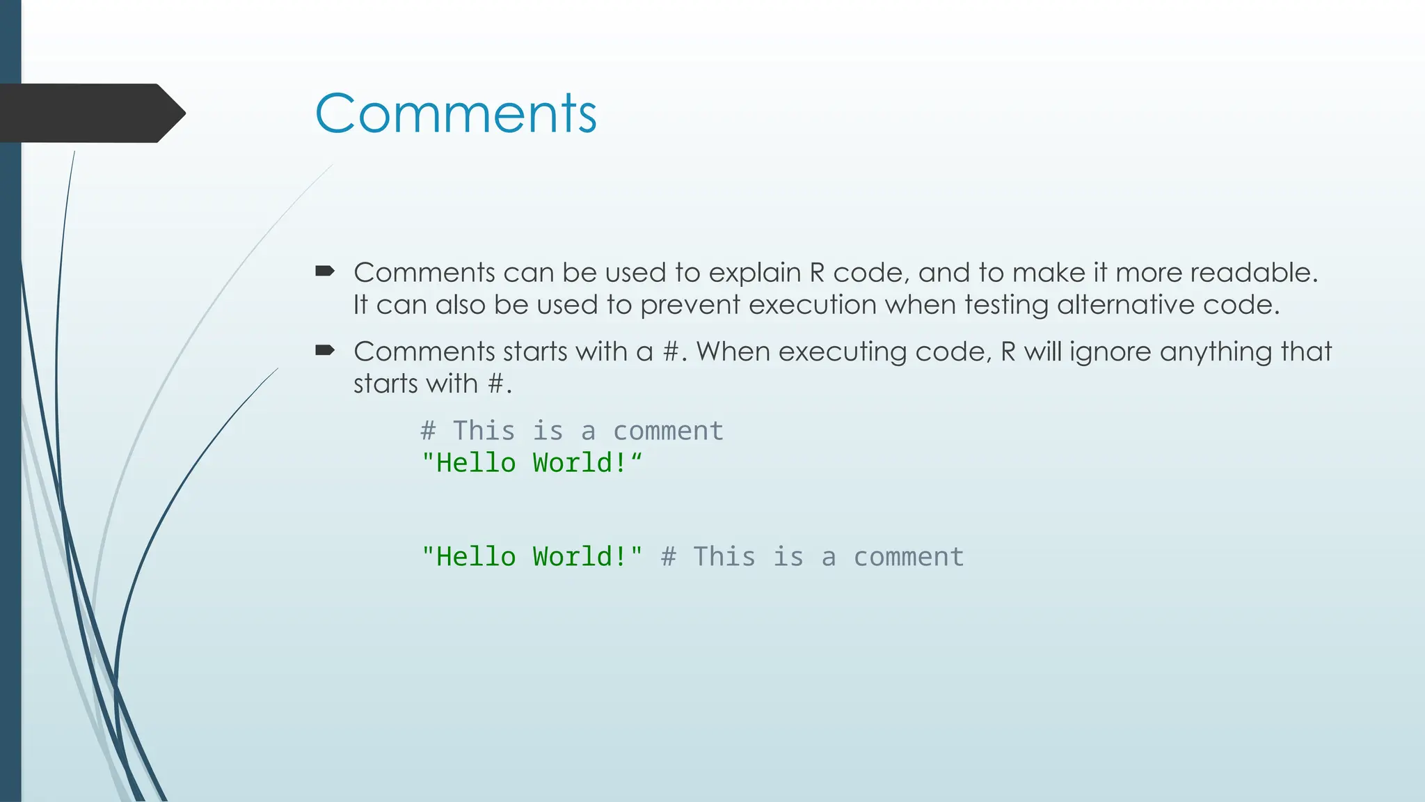
Comments
Comments canbe used to explain R code, and to make it more readable.
It can also be used to prevent execution when testing alternative code.
Comments starts with a #. When executing code, R will ignore anything that
starts with #.
# This is a comment
"Hello World!“
"Hello World!" # This is a comment
25.
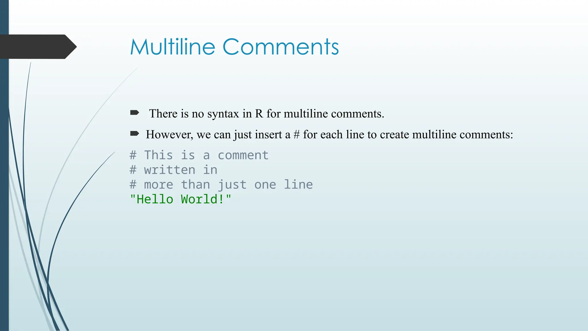
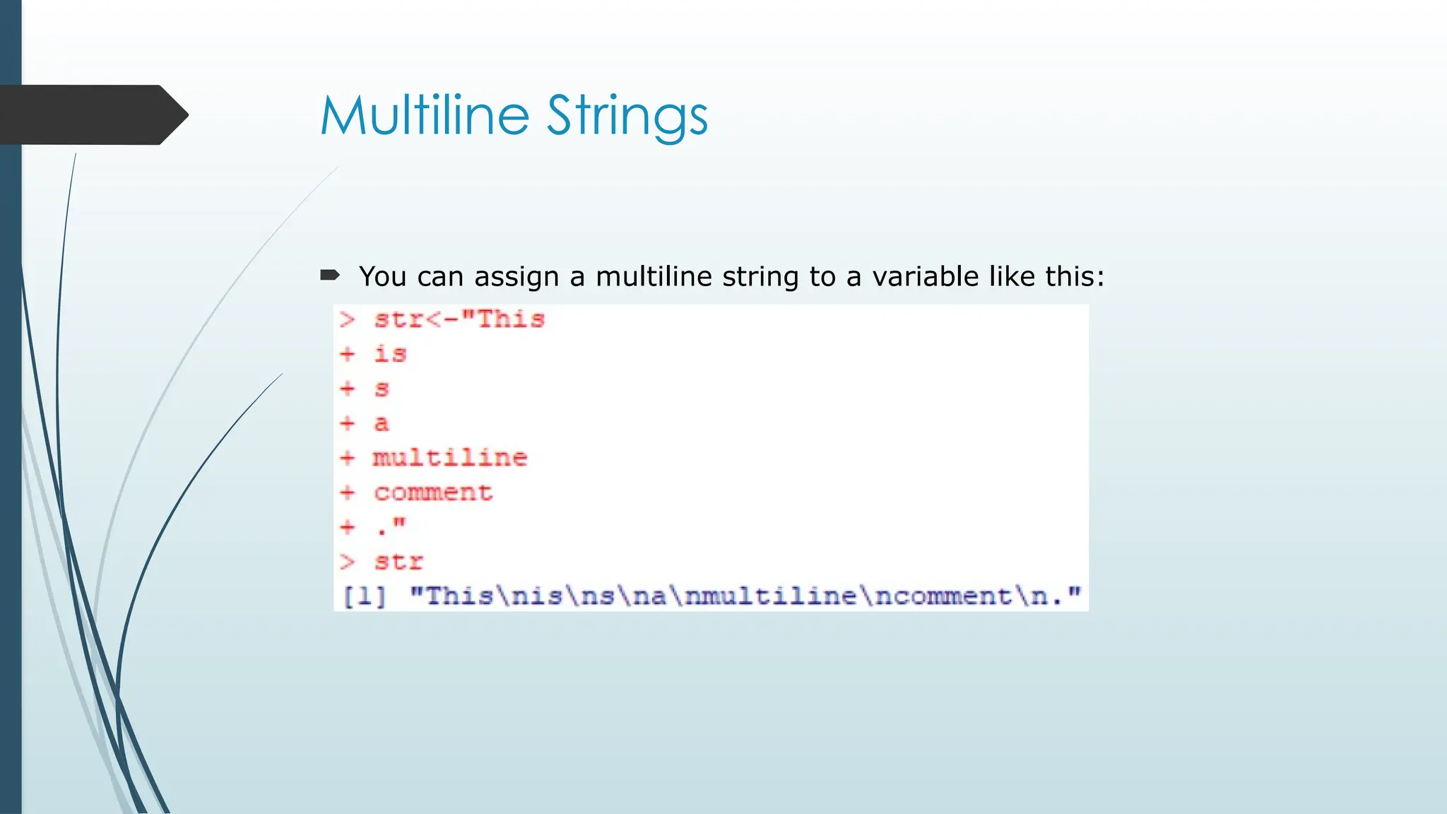
Multiline Comments
Thereis no syntax in R for multiline comments.
However, we can just insert a # for each line to create multiline comments:
# This is a comment
# written in
# more than just one line
"Hello World!"
26.
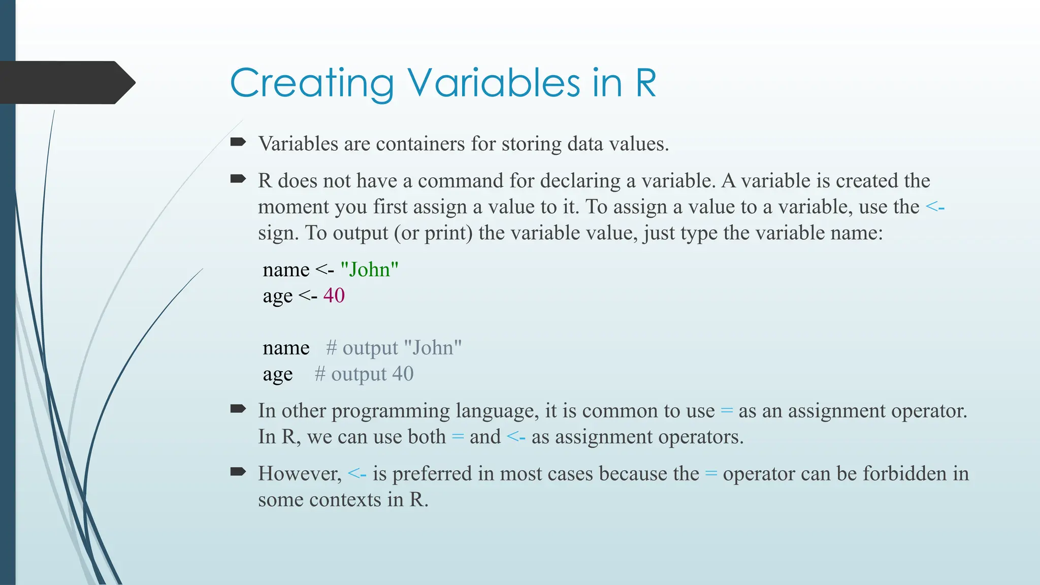
Creating Variables inR
Variables are containers for storing data values.
R does not have a command for declaring a variable. A variable is created the
moment you first assign a value to it. To assign a value to a variable, use the <-
sign. To output (or print) the variable value, just type the variable name:
name <- "John"
age <- 40
name # output "John"
age # output 40
In other programming language, it is common to use = as an assignment operator.
In R, we can use both = and <- as assignment operators.
However, <- is preferred in most cases because the = operator can be forbidden in
some contexts in R.
27.
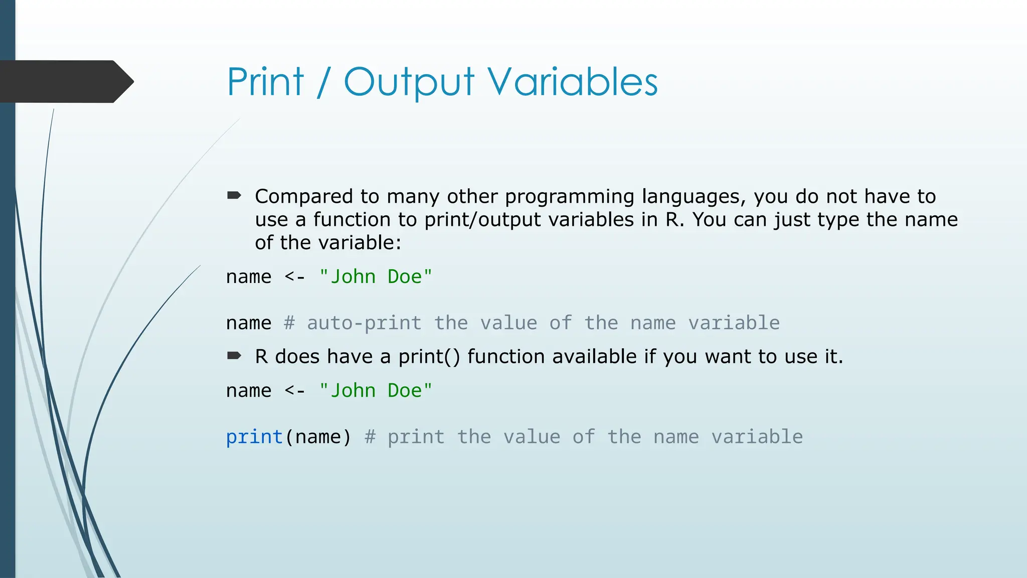
Print / OutputVariables
Compared to many other programming languages, you do not have to
use a function to print/output variables in R. You can just type the name
of the variable:
name <- "John Doe"
name # auto-print the value of the name variable
R does have a print() function available if you want to use it.
name <- "John Doe"
print(name) # print the value of the name variable
28.
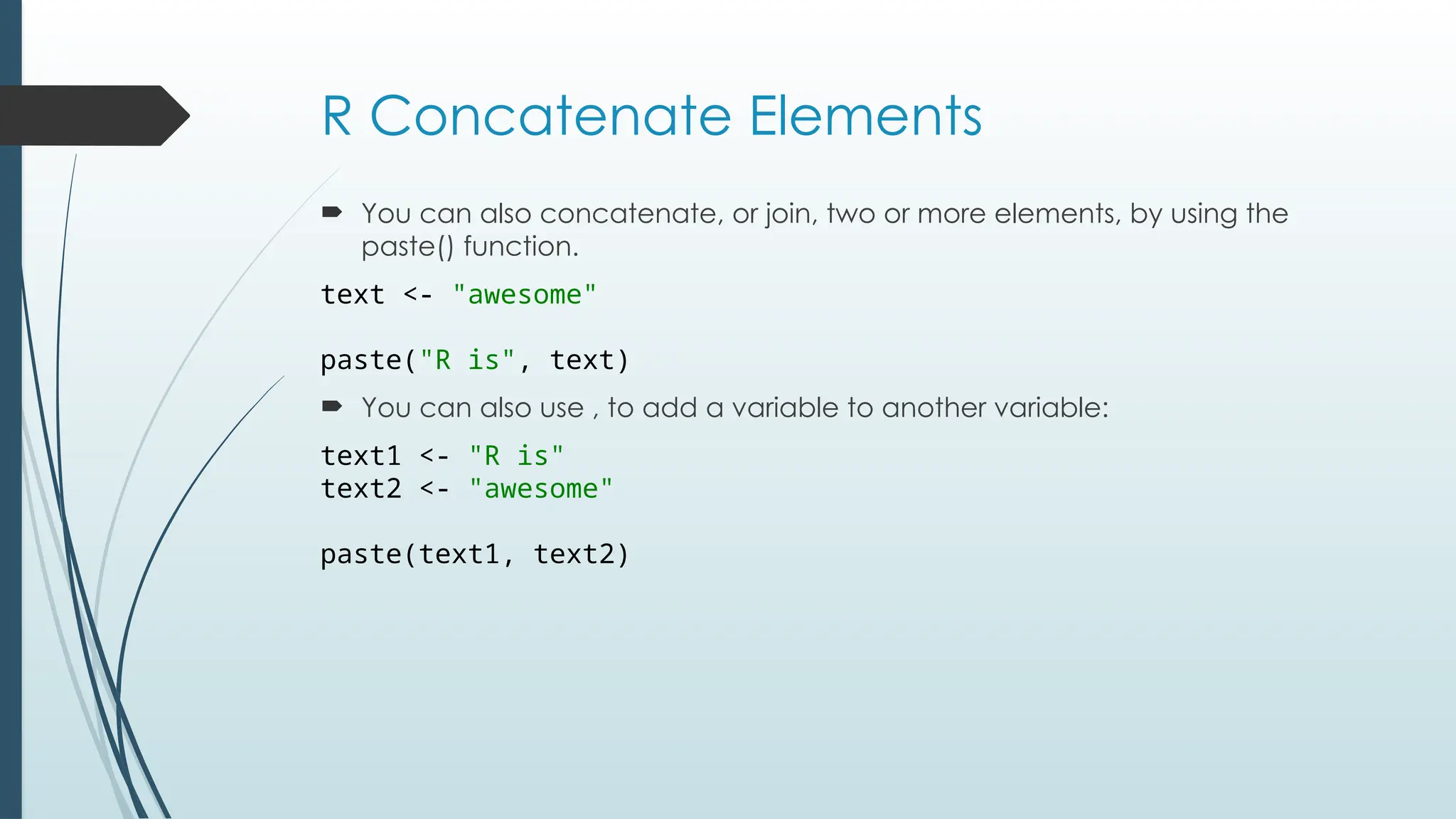
R Concatenate Elements
You can also concatenate, or join, two or more elements, by using the
paste() function.
text <- "awesome"
paste("R is", text)
You can also use , to add a variable to another variable:
text1 <- "R is"
text2 <- "awesome"
paste(text1, text2)
29.
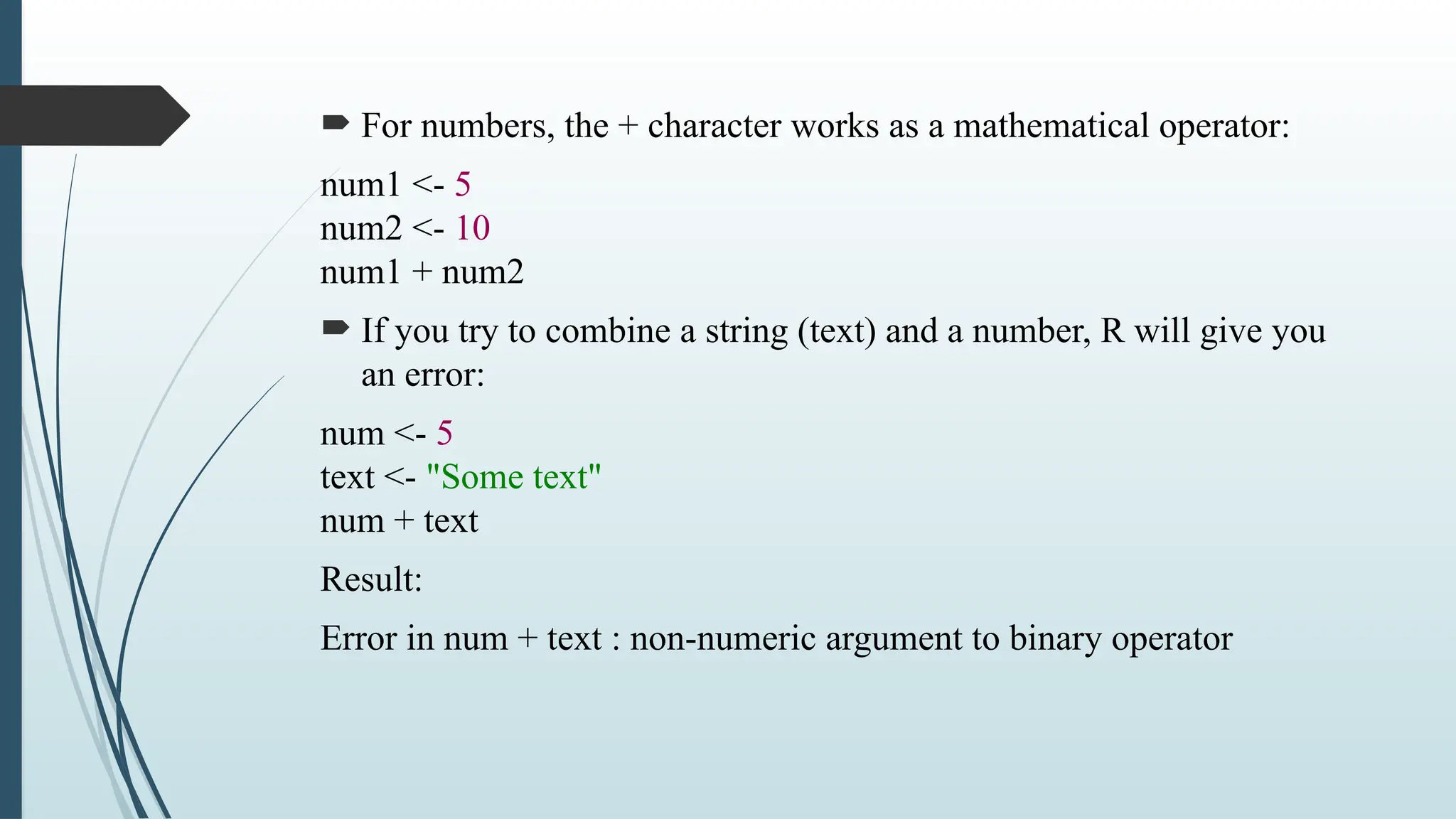
For numbers,the + character works as a mathematical operator:
num1 <- 5
num2 <- 10
num1 + num2
If you try to combine a string (text) and a number, R will give you
an error:
num <- 5
text <- "Some text"
num + text
Result:
Error in num + text : non-numeric argument to binary operator
30.
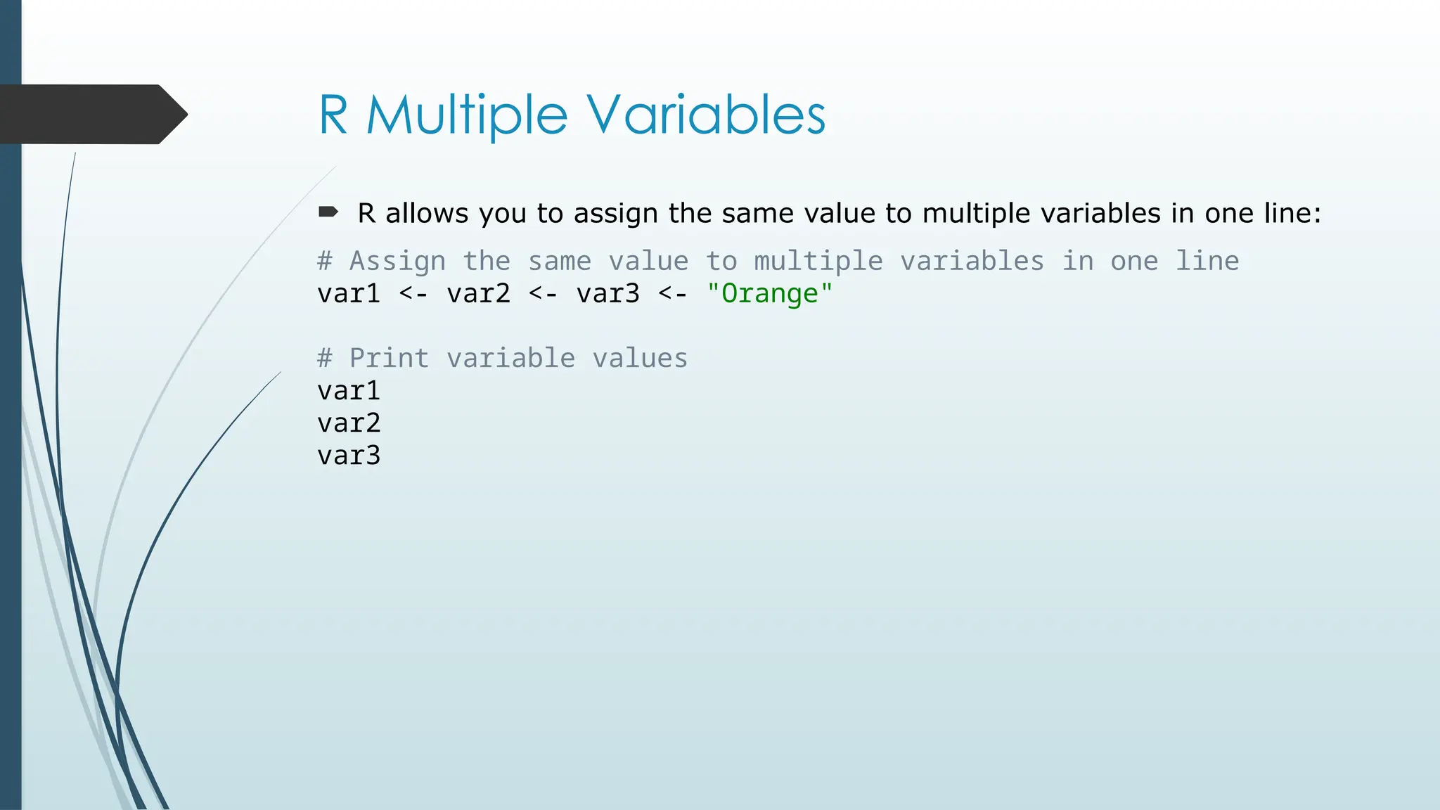
R Multiple Variables
R allows you to assign the same value to multiple variables in one line:
# Assign the same value to multiple variables in one line
var1 <- var2 <- var3 <- "Orange"
# Print variable values
var1
var2
var3
31.
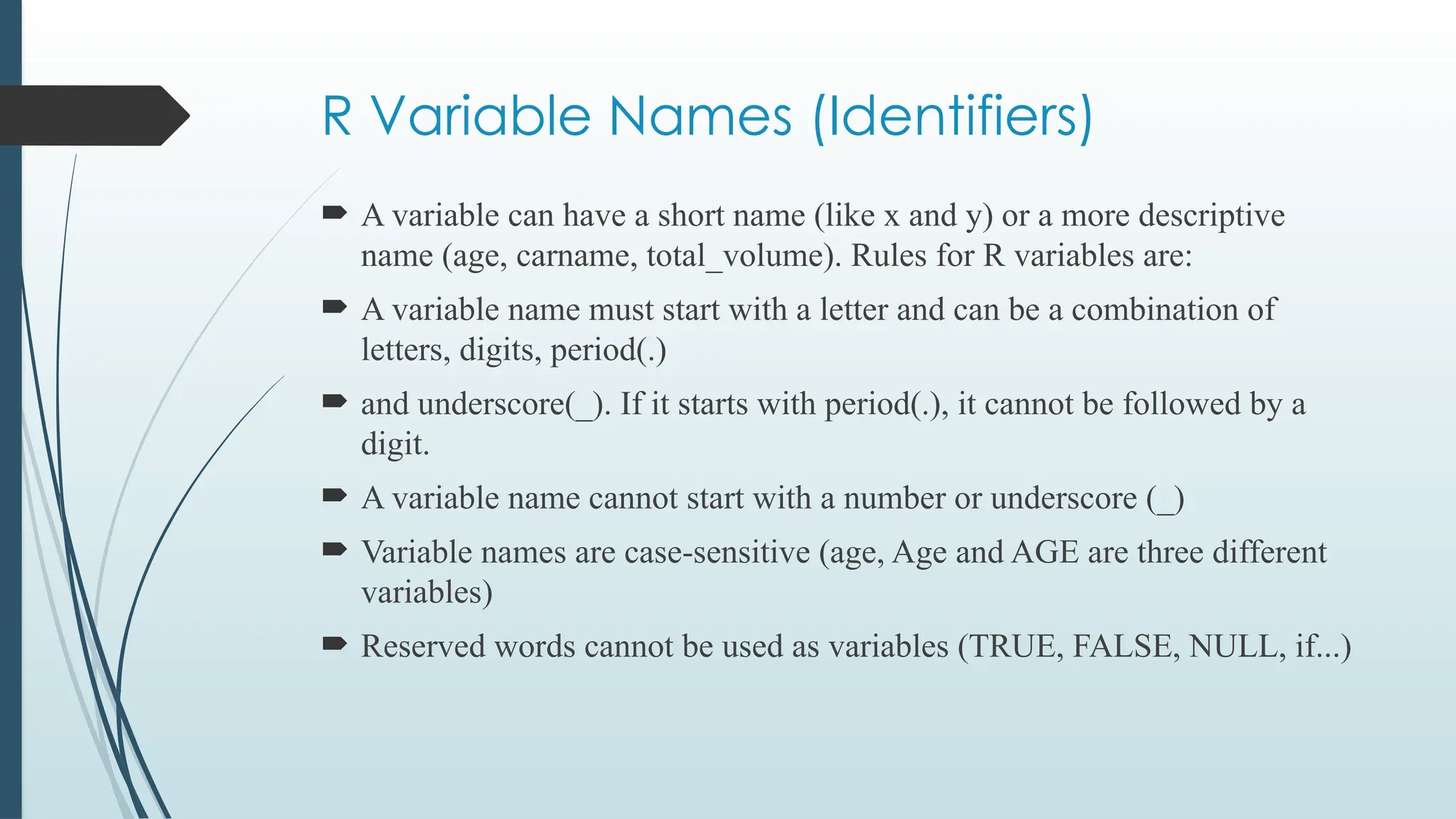
R Variable Names(Identifiers)
A variable can have a short name (like x and y) or a more descriptive
name (age, carname, total_volume). Rules for R variables are:
A variable name must start with a letter and can be a combination of
letters, digits, period(.)
and underscore(_). If it starts with period(.), it cannot be followed by a
digit.
A variable name cannot start with a number or underscore (_)
Variable names are case-sensitive (age, Age and AGE are three different
variables)
Reserved words cannot be used as variables (TRUE, FALSE, NULL, if...)
Basic Data Types
numeric - (10.5, 55, 787)
integer - (1L, 55L, 100L, where the letter "L" declares this as an
integer)
complex - (9 + 3i, where "i" is the imaginary part)
character (string) - ("k", "R is exciting", "FALSE", "11.5")
logical (boolean) - (TRUE or FALSE)
34.
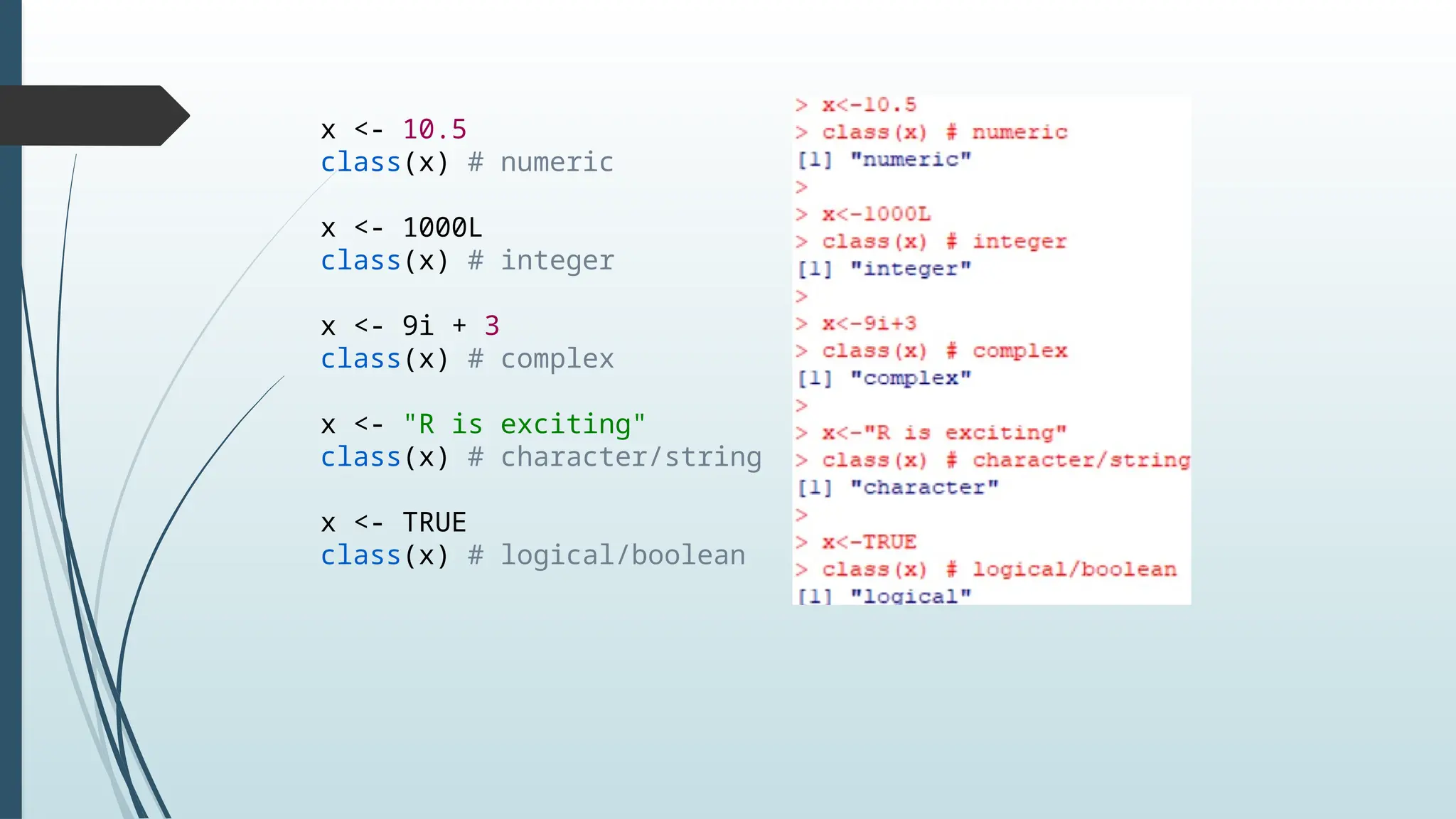
x <- 10.5
class(x)# numeric
x <- 1000L
class(x) # integer
x <- 9i + 3
class(x) # complex
x <- "R is exciting"
class(x) # character/string
x <- TRUE
class(x) # logical/boolean
35.
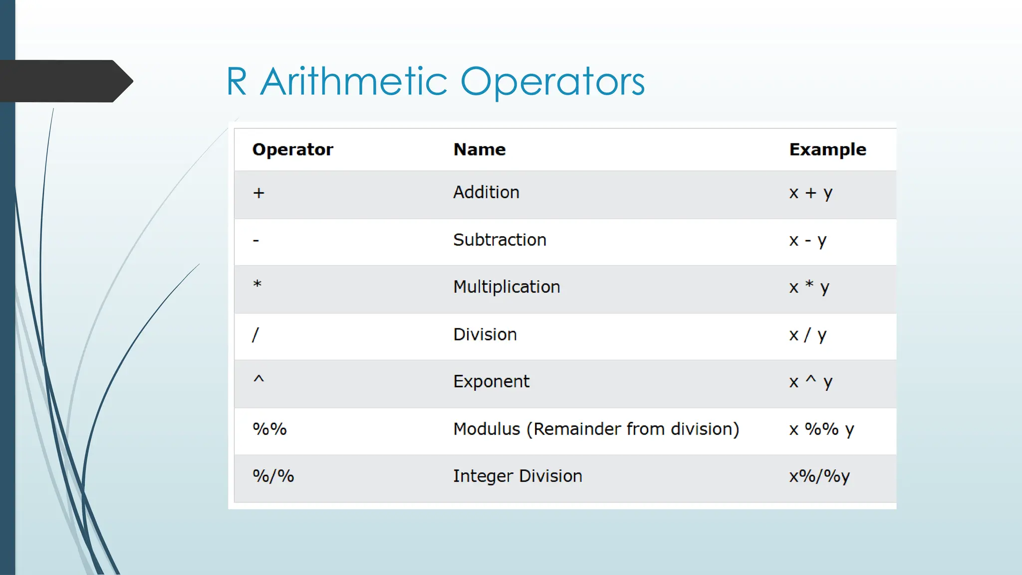
Simple Math
InR, you can use operators to perform common mathematical
operations on numbers.
The + operator is used to add together two values:
10+5
And the - operator is used for subtraction:
10-5
36.
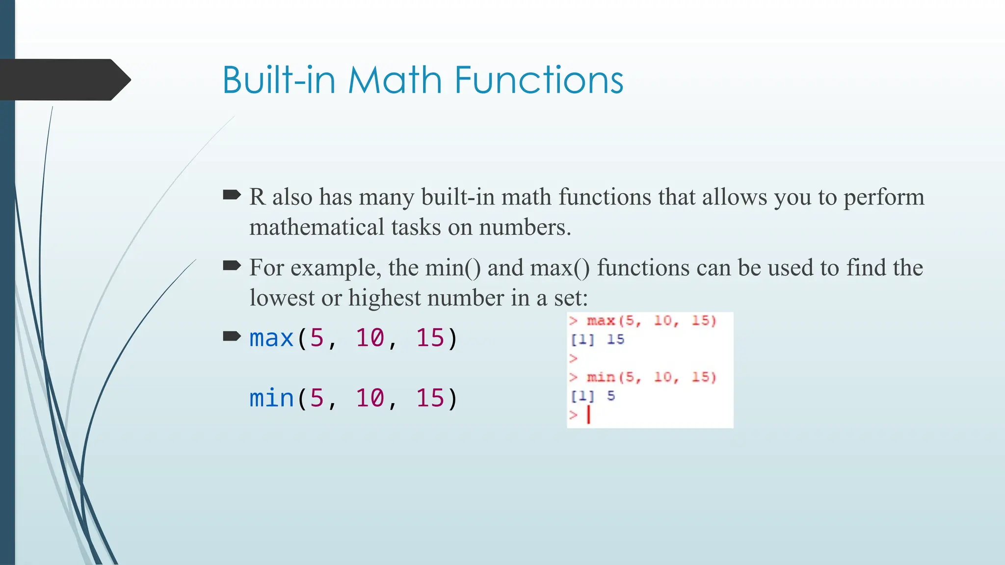
Built-in Math Functions
R also has many built-in math functions that allows you to perform
mathematical tasks on numbers.
For example, the min() and max() functions can be used to find the
lowest or highest number in a set:
max(5, 10, 15)
min(5, 10, 15)
37.
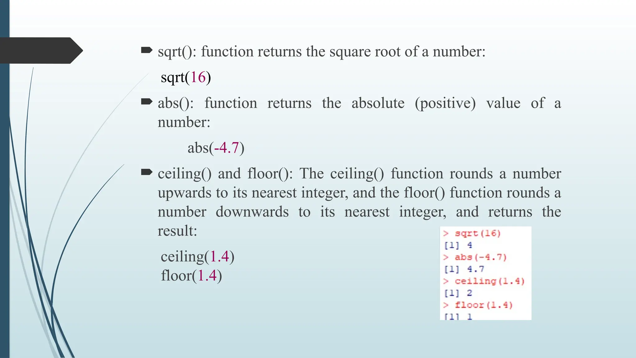
sqrt(): functionreturns the square root of a number:
sqrt(16)
abs(): function returns the absolute (positive) value of a
number:
abs(-4.7)
ceiling() and floor(): The ceiling() function rounds a number
upwards to its nearest integer, and the floor() function rounds a
number downwards to its nearest integer, and returns the
result:
ceiling(1.4)
floor(1.4)
38.
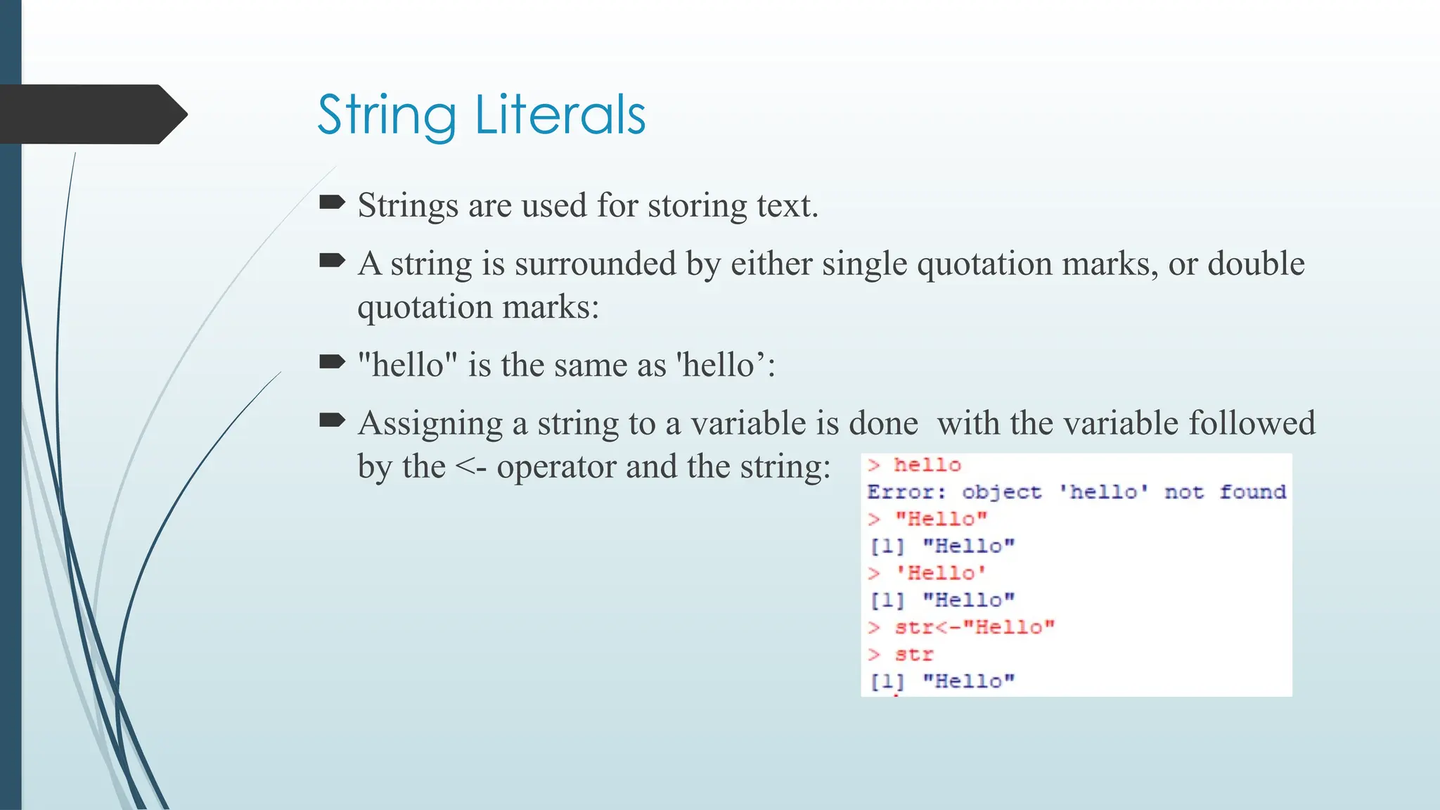
String Literals
Stringsare used for storing text.
A string is surrounded by either single quotation marks, or double
quotation marks:
"hello" is the same as 'hello’:
Assigning a string to a variable is done with the variable followed
by the <- operator and the string:
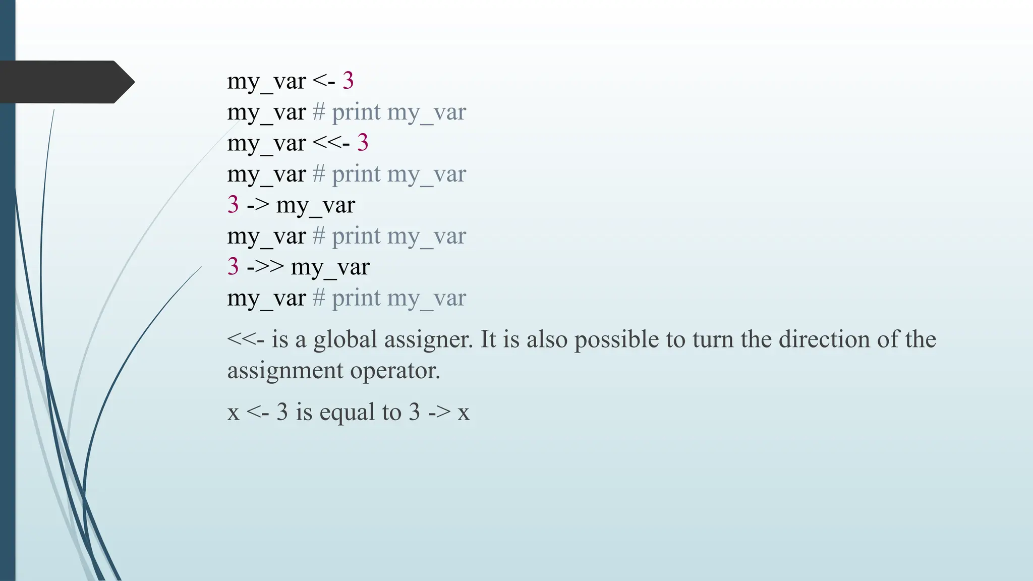
my_var <- 3
my_var# print my_var
my_var <<- 3
my_var # print my_var
3 -> my_var
my_var # print my_var
3 ->> my_var
my_var # print my_var
<<- is a global assigner. It is also possible to turn the direction of the
assignment operator.
x <- 3 is equal to 3 -> x
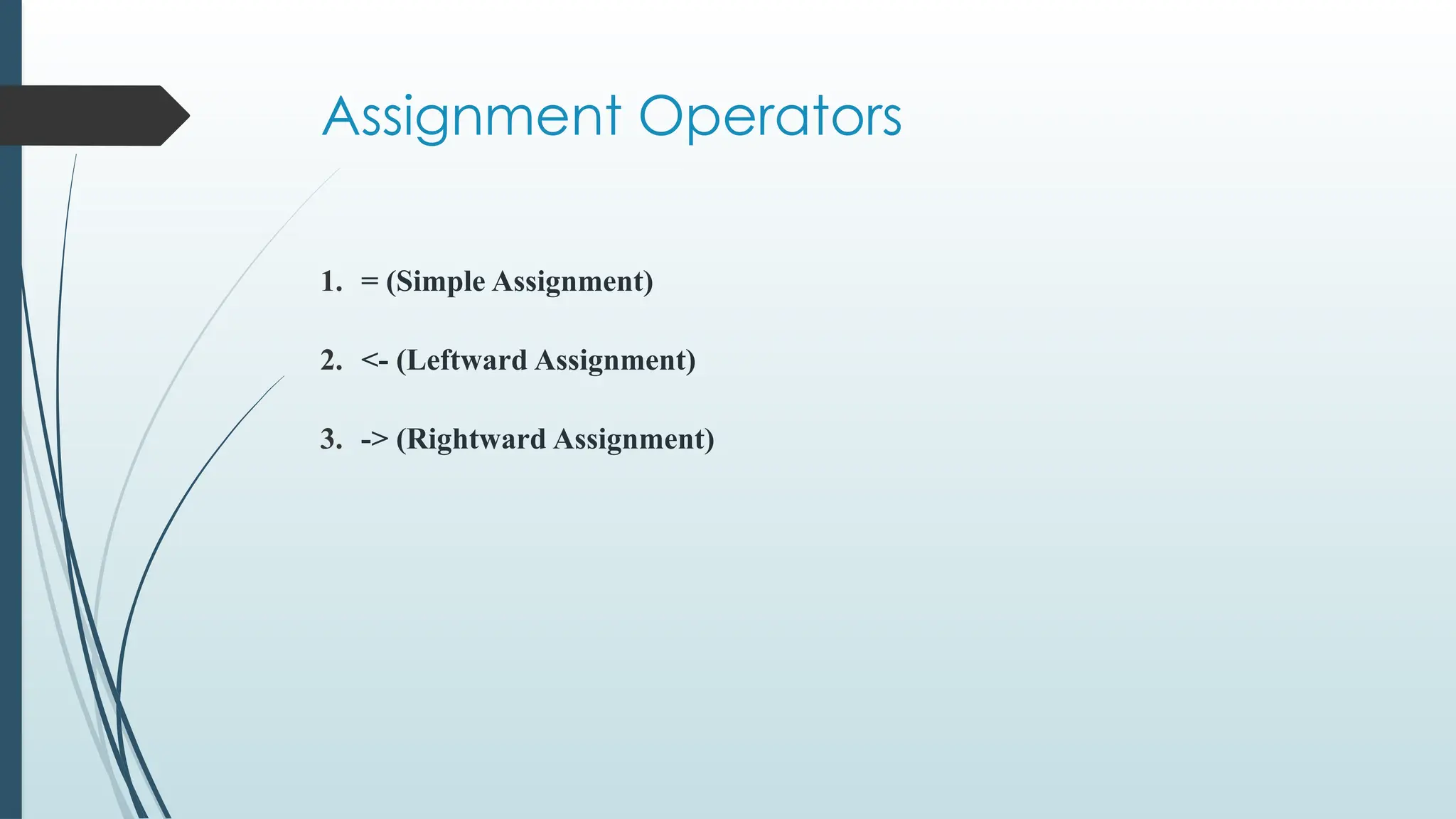
47.
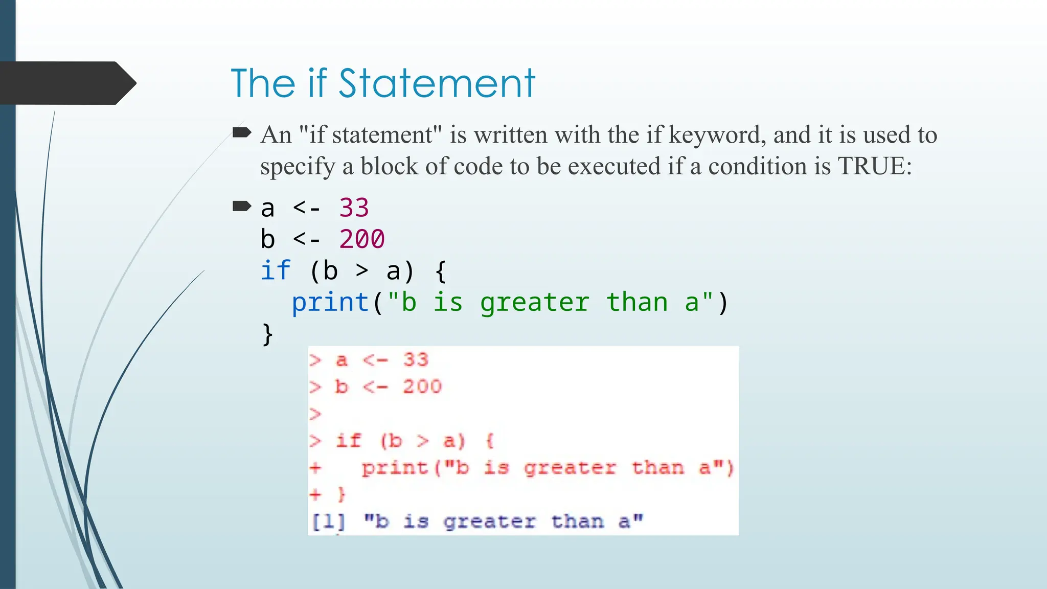
The if Statement
An "if statement" is written with the if keyword, and it is used to
specify a block of code to be executed if a condition is TRUE:
a <- 33
b <- 200
if (b > a) {
print("b is greater than a")
}
48.
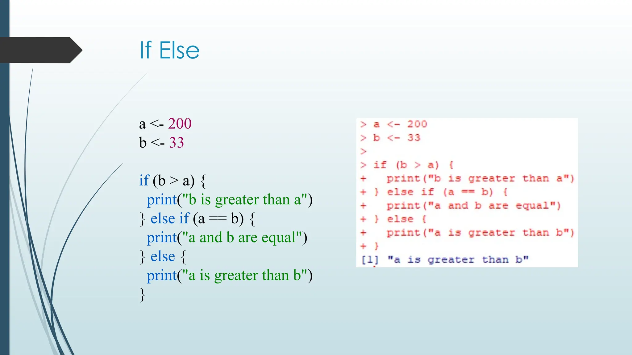
If Else
a <-200
b <- 33
if (b > a) {
print("b is greater than a")
} else if (a == b) {
print("a and b are equal")
} else {
print("a is greater than b")
}
49.
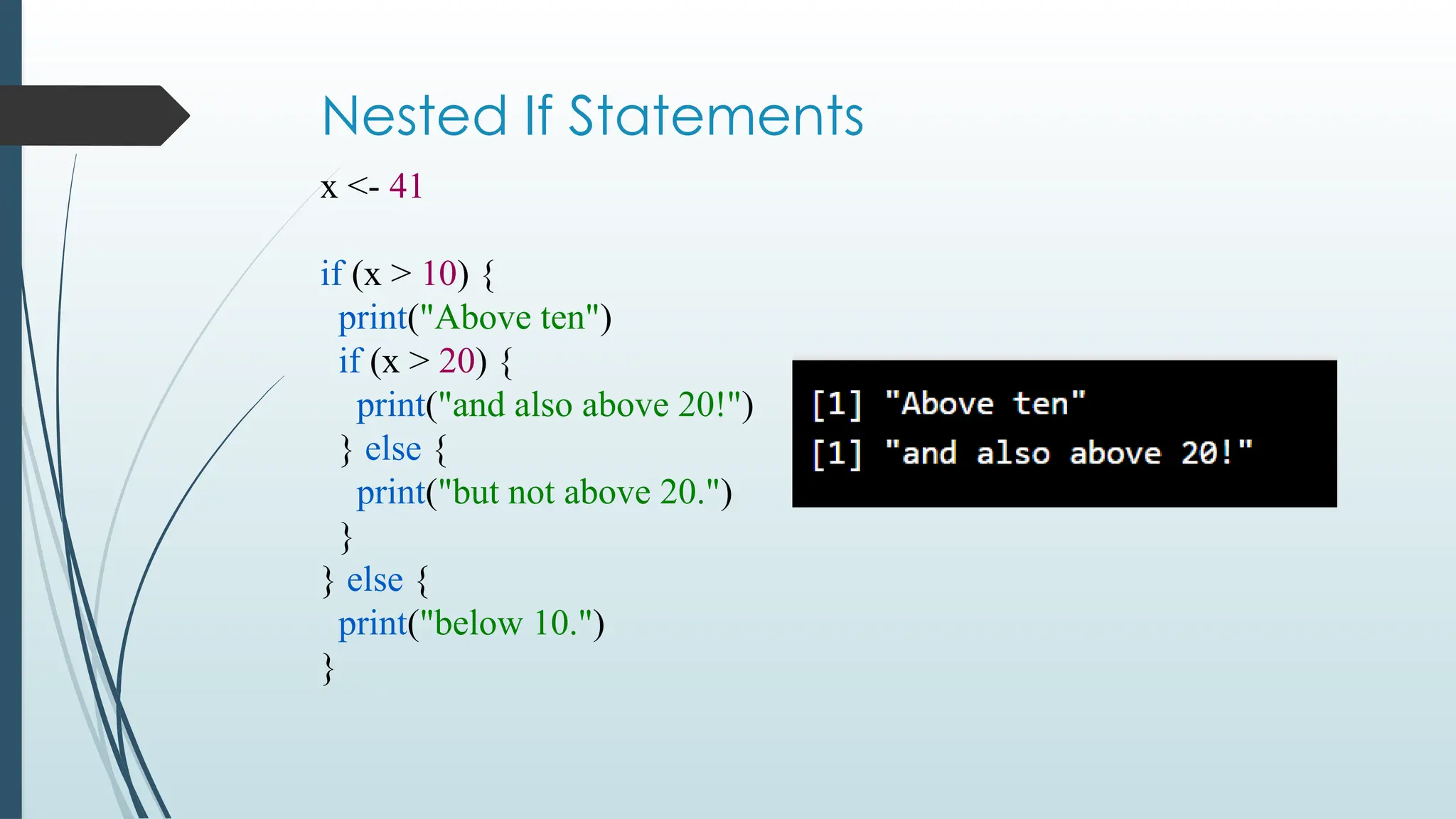
Nested If Statements
x<- 41
if (x > 10) {
print("Above ten")
if (x > 20) {
print("and also above 20!")
} else {
print("but not above 20.")
}
} else {
print("below 10.")
}
50.
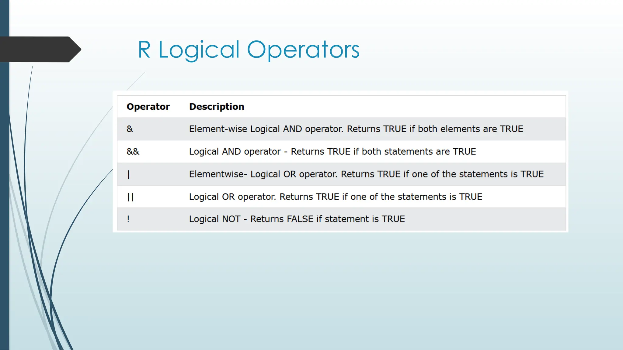
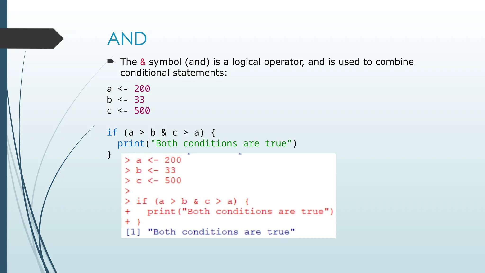
AND
The &symbol (and) is a logical operator, and is used to combine
conditional statements:
a <- 200
b <- 33
c <- 500
if (a > b & c > a) {
print("Both conditions are true")
}
51.
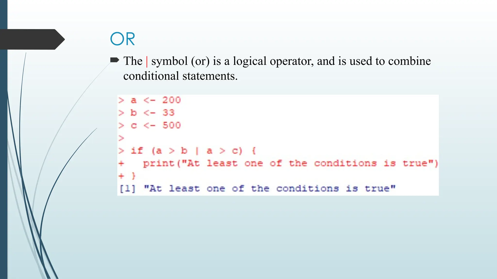
OR
The |symbol (or) is a logical operator, and is used to combine
conditional statements.
52.
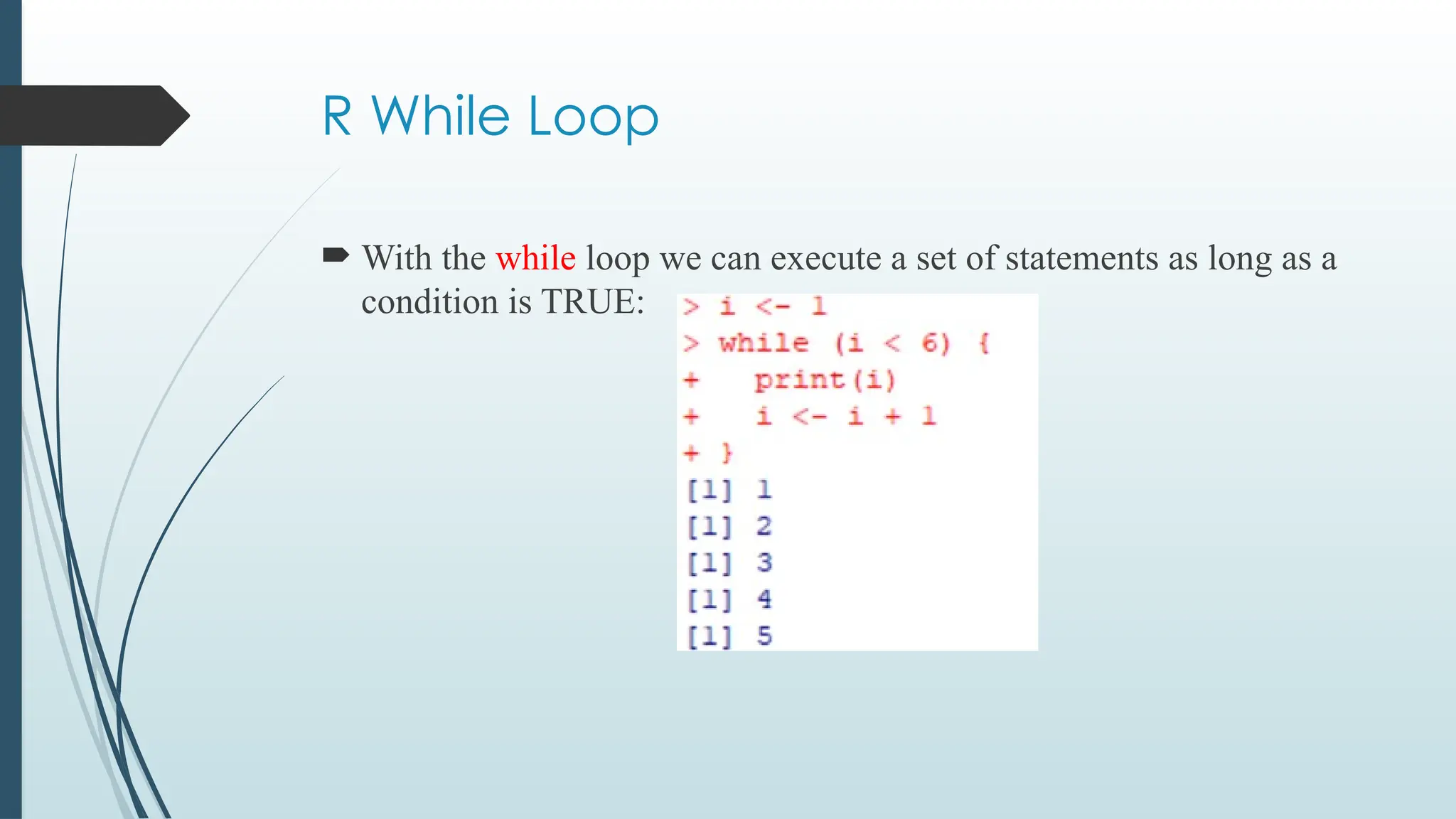
R While Loop
With the while loop we can execute a set of statements as long as a
condition is TRUE:
53.
Break
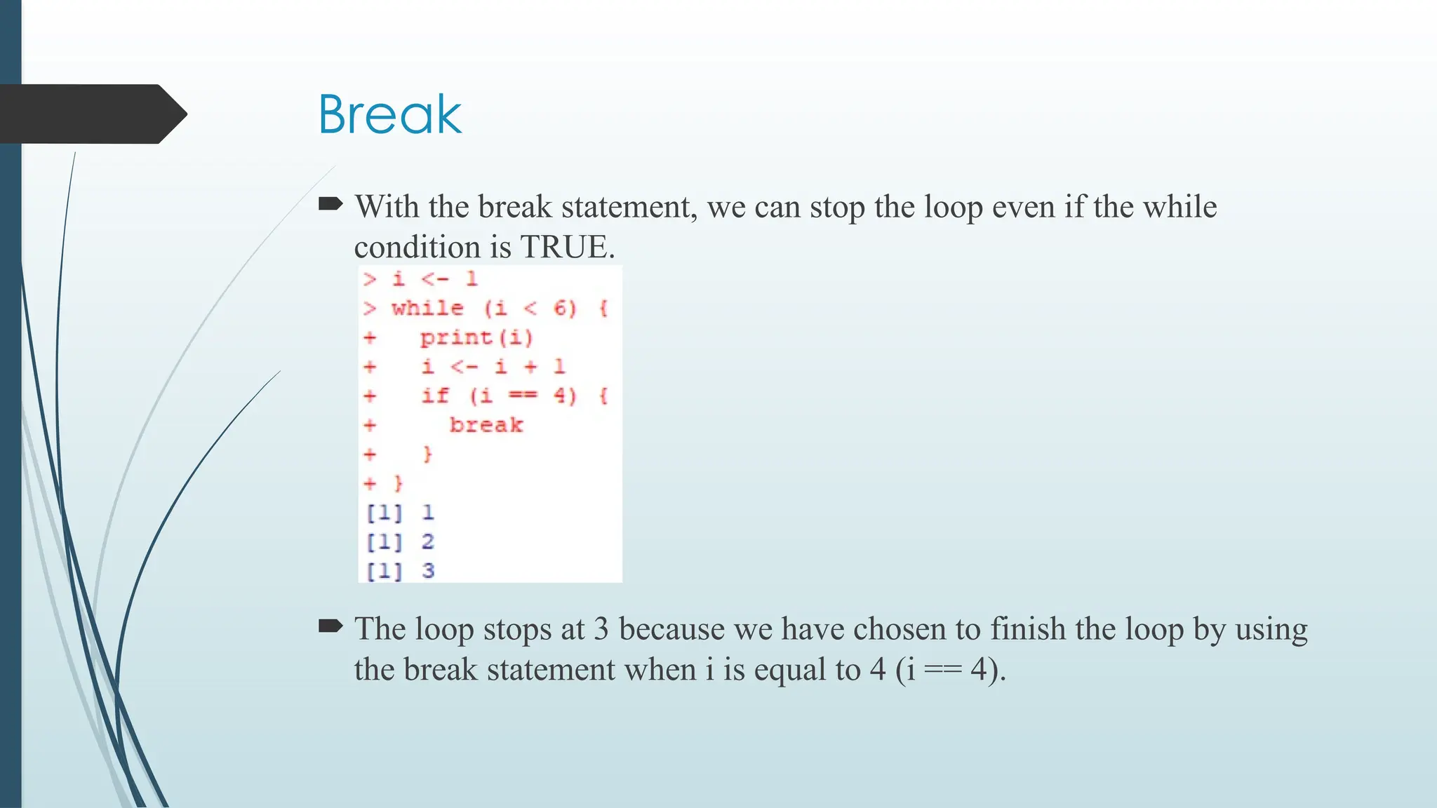
With thebreak statement, we can stop the loop even if the while
condition is TRUE.
The loop stops at 3 because we have chosen to finish the loop by using
the break statement when i is equal to 4 (i == 4).
54.
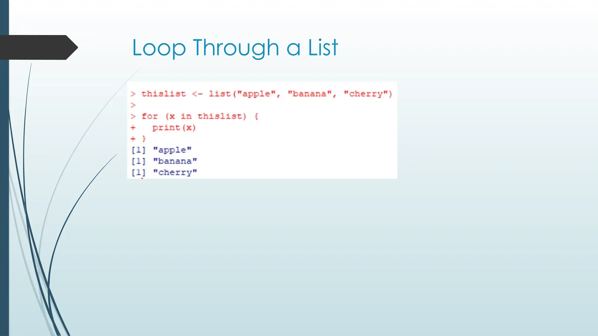
For Loop
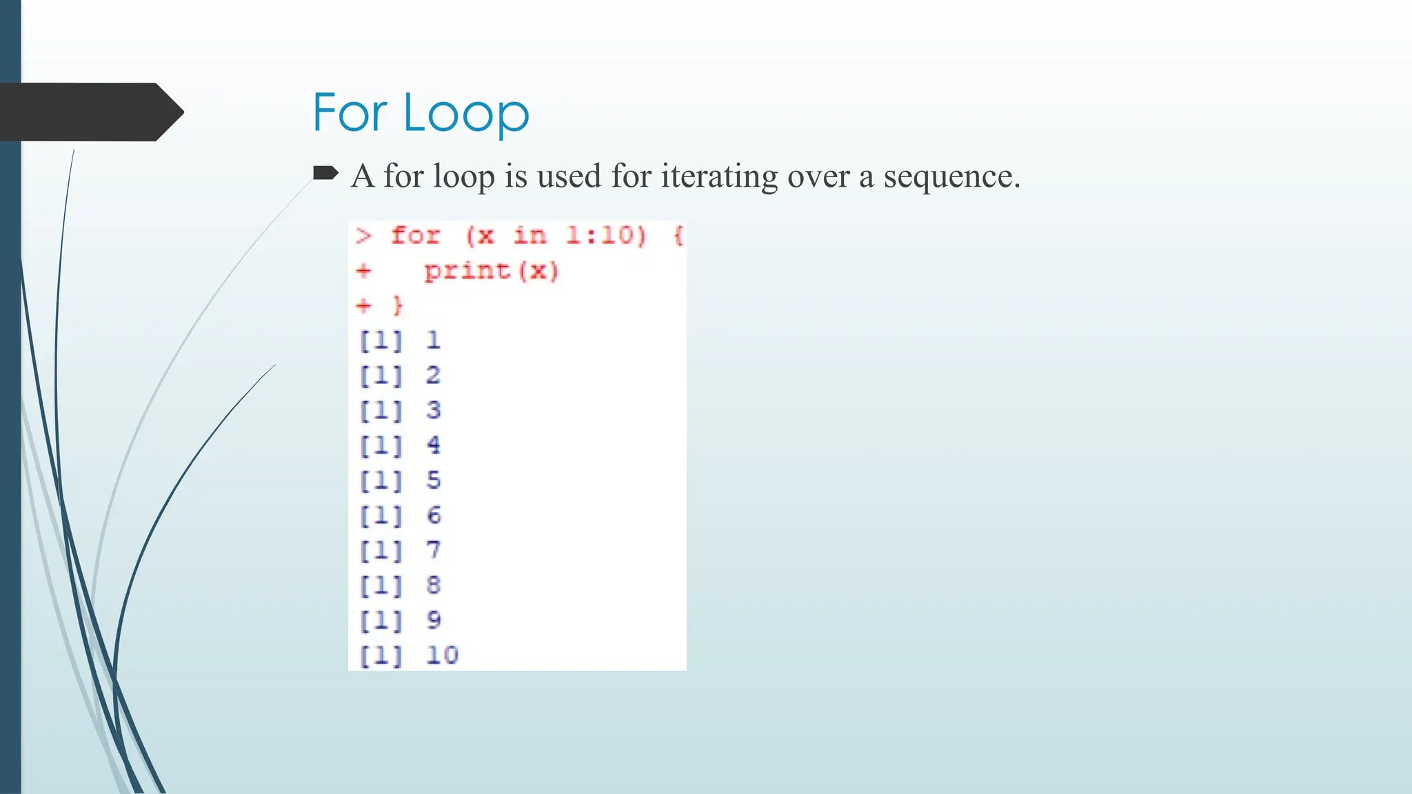
Afor loop is used for iterating over a sequence.
55.
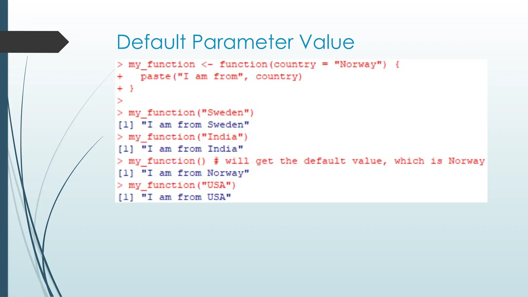
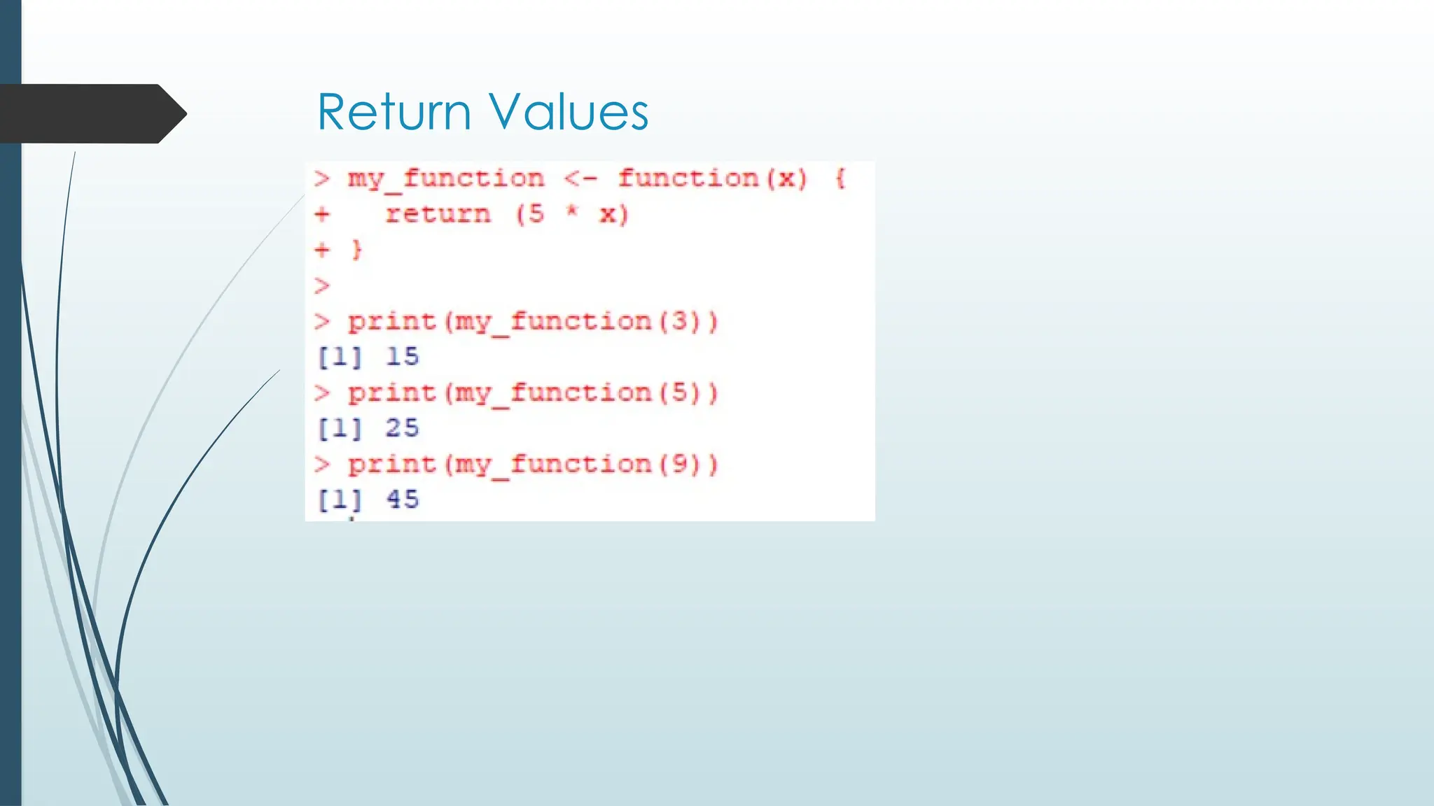
Functions in R
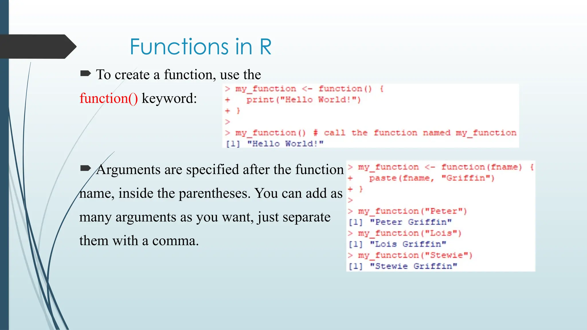
To create a function, use the
function() keyword:
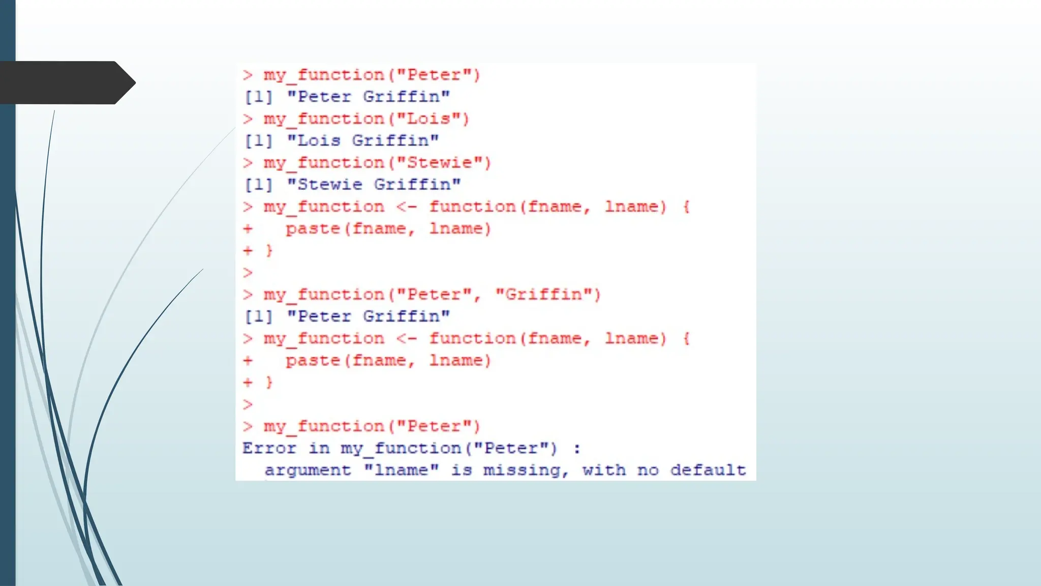
Arguments are specified after the function
name, inside the parentheses. You can add as
many arguments as you want, just separate
them with a comma.
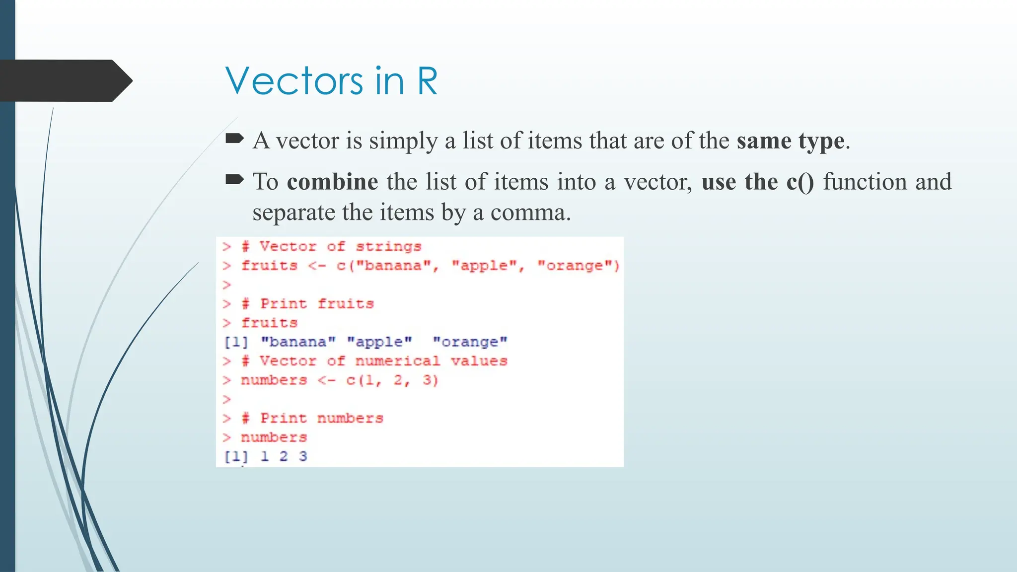
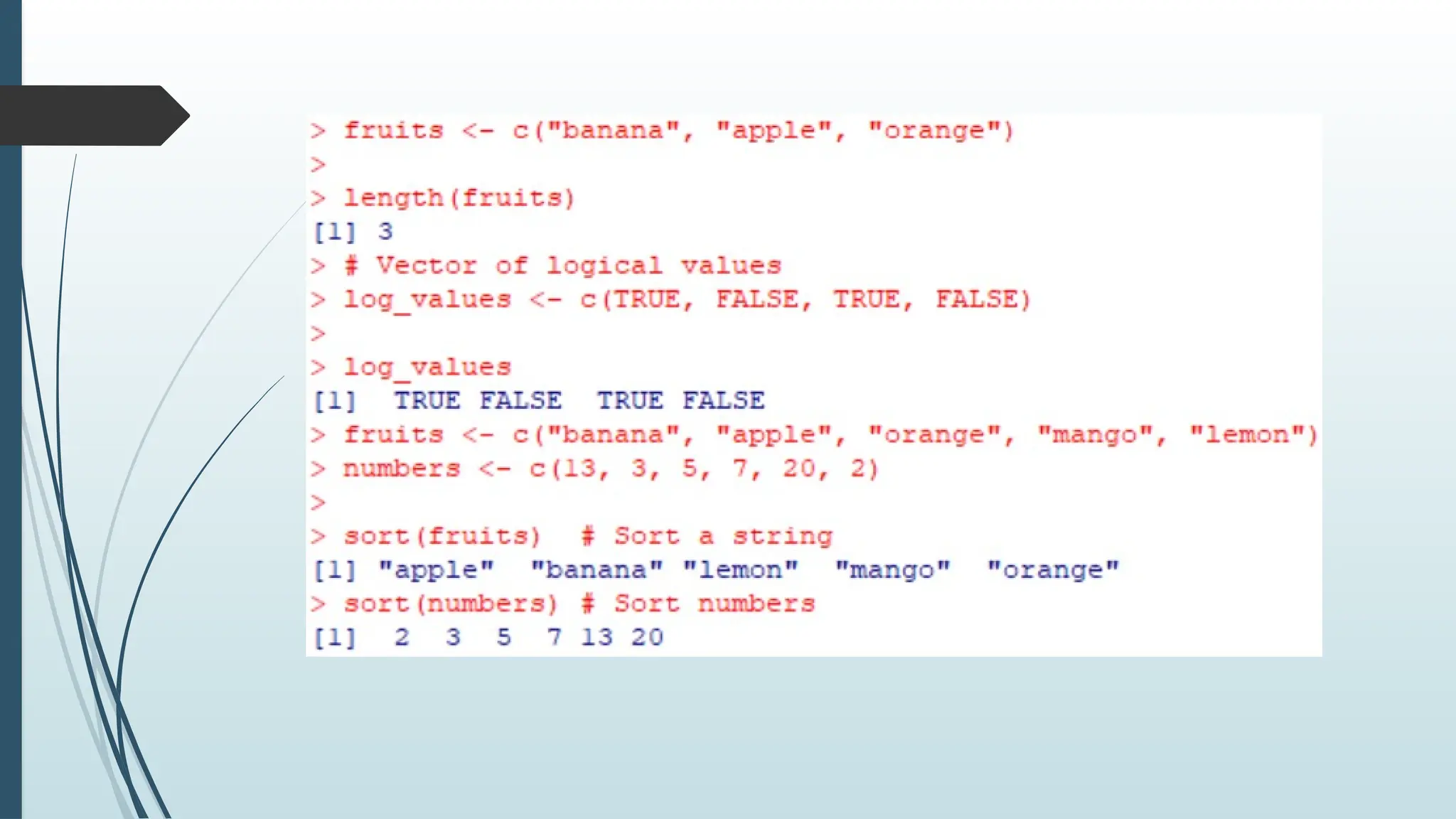
Vectors in R
A vector is simply a list of items that are of the same type.
To combine the list of items into a vector, use the c() function and
separate the items by a comma.
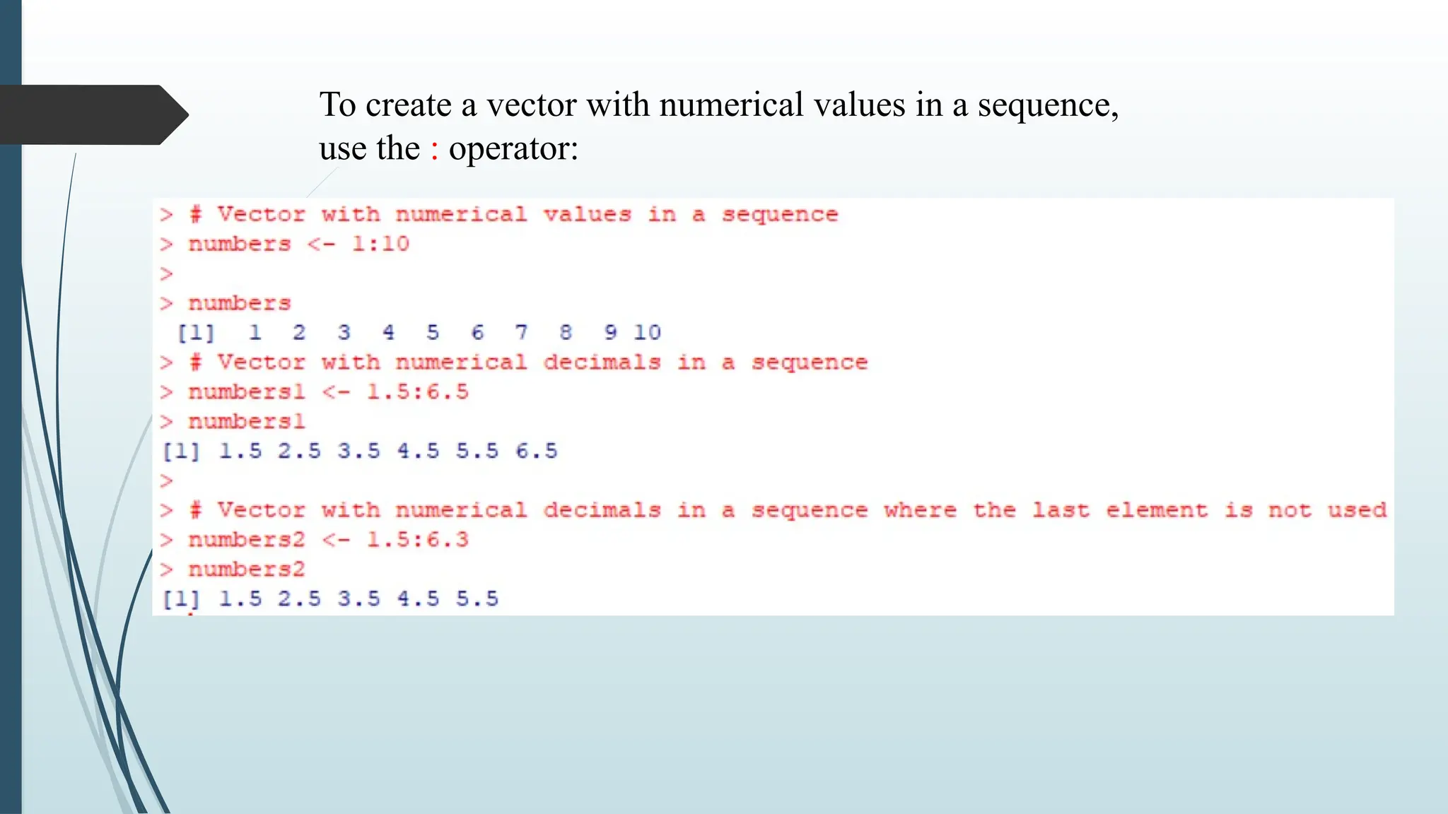
61.
To create avector with numerical values in a sequence,
use the : operator:
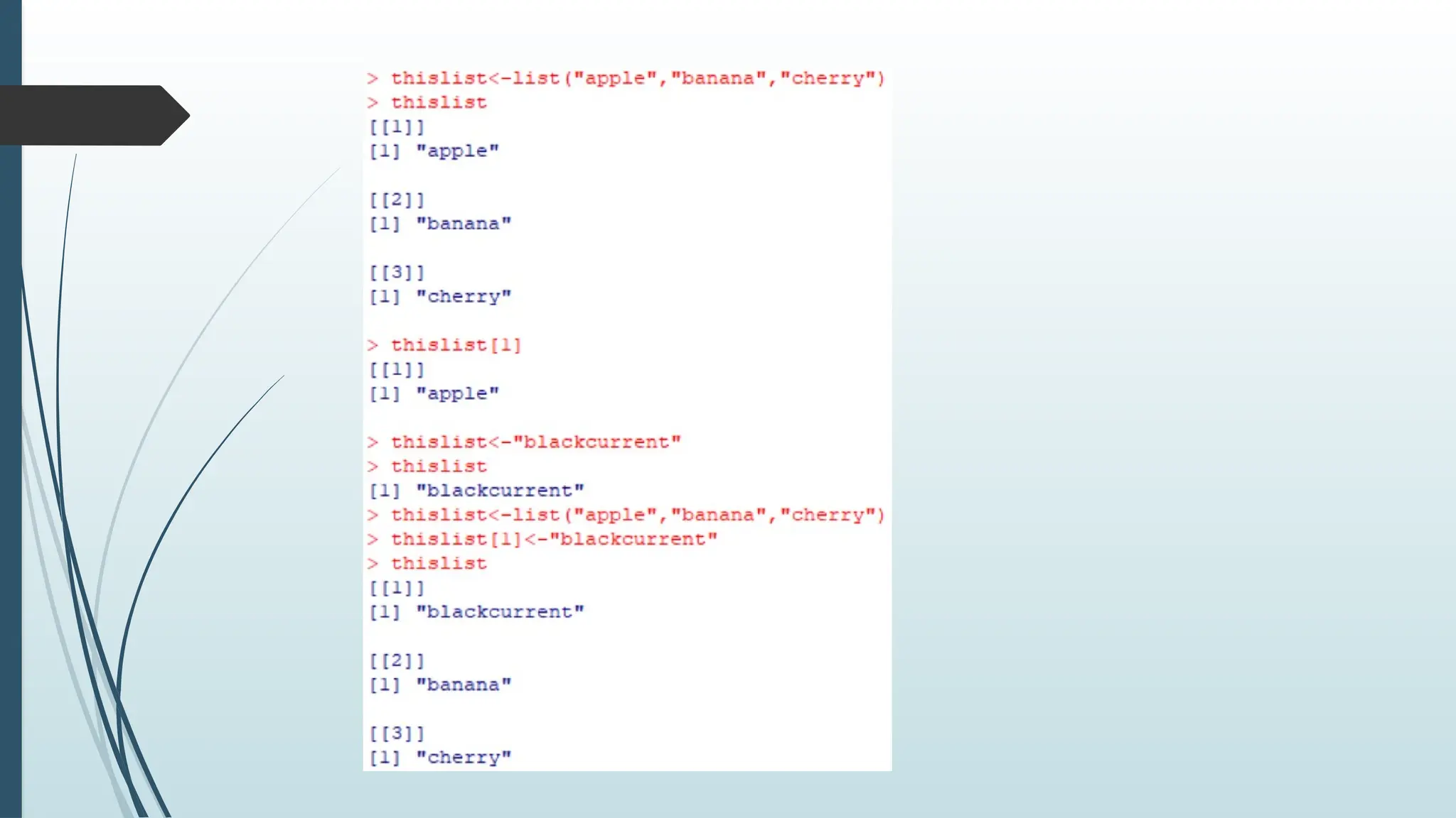
R Lists
Alist in R can contain many different data types inside it. A list is a
collection of data which is ordered and changeable.
# List of strings
thislist <- list("apple", "banana", "cherry")
# Print the list
thislist
thislist[1]
thislist[1] <- "blackcurrant"
# Print the updated list
thislist
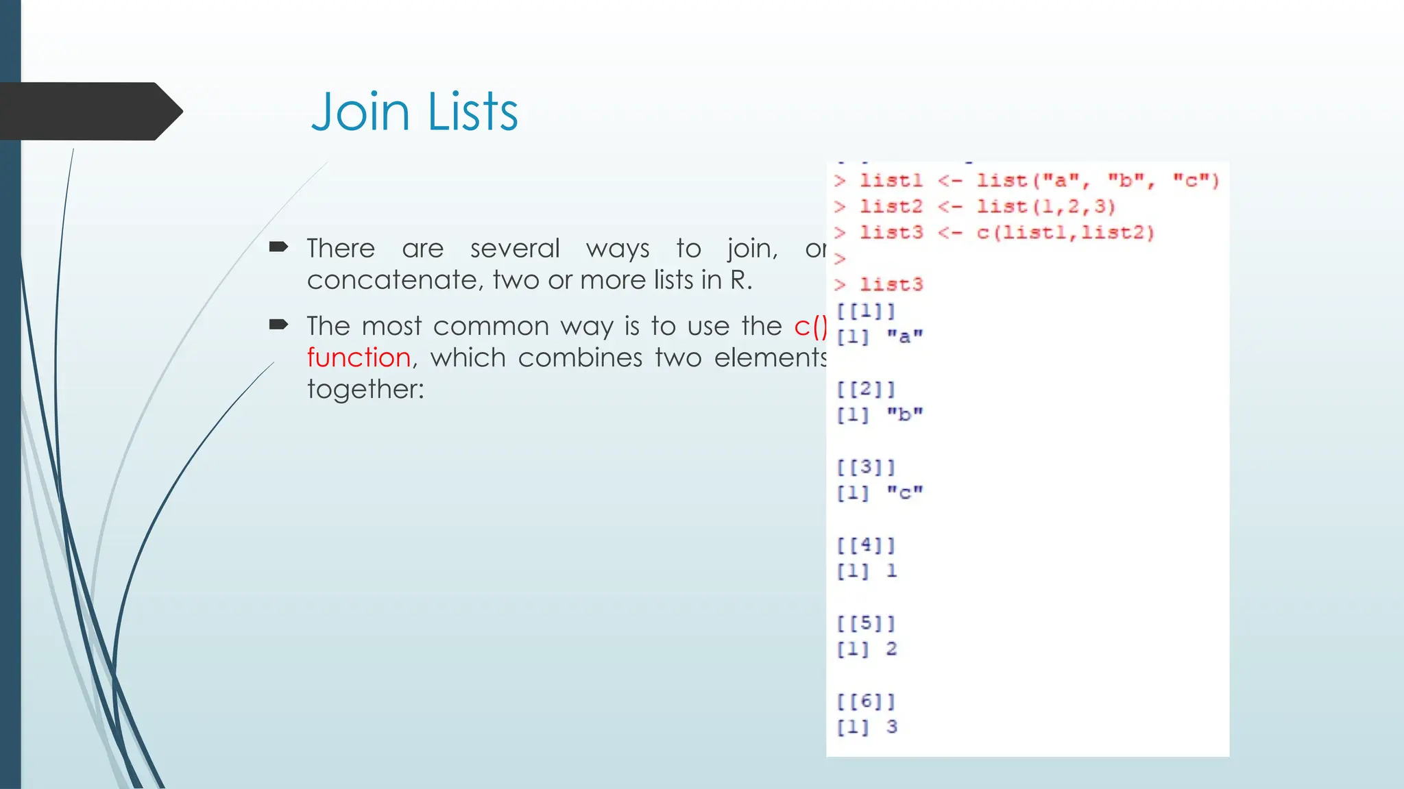
Join Lists
Thereare several ways to join, or
concatenate, two or more lists in R.
The most common way is to use the c()
function, which combines two elements
together:
72.
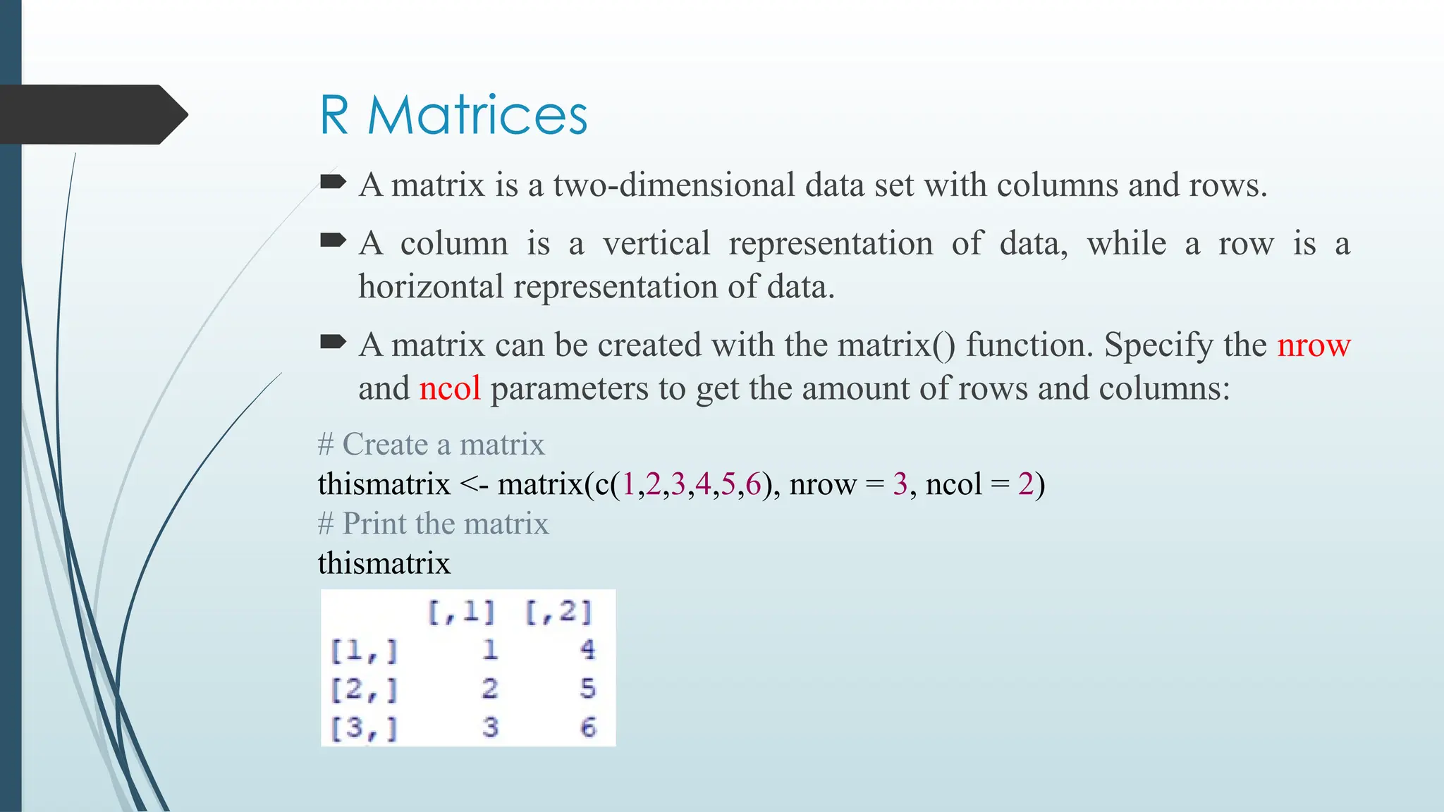
R Matrices
Amatrix is a two-dimensional data set with columns and rows.
A column is a vertical representation of data, while a row is a
horizontal representation of data.
A matrix can be created with the matrix() function. Specify the nrow
and ncol parameters to get the amount of rows and columns:
# Create a matrix
thismatrix <- matrix(c(1,2,3,4,5,6), nrow = 3, ncol = 2)
# Print the matrix
thismatrix
73.
Creating a stringtype matrix
thismatrix <- matrix(c("apple", "banana", "cherry", "orange"), nrow = 2, ncol = 2)
thismatrix
You can access the items by using [ ] brackets. The first number "1" in the bracket
specifies the row-position, while the second number "2" specifies the column-
position:
74.
The whole rowcan be accessed if you specify a comma after the
number in the bracket:
The whole column can be accessed if you specify a comma before the
number in the bracket:
More than one row can be accessed if you use the c() function:
thismatrix <- matrix(c("apple", "banana", "cherry", "orange", "grape",
"pineapple", "pear", "melon", "fig"), nrow = 3, ncol = 3)
thismatrix[c(1,2),]
75.
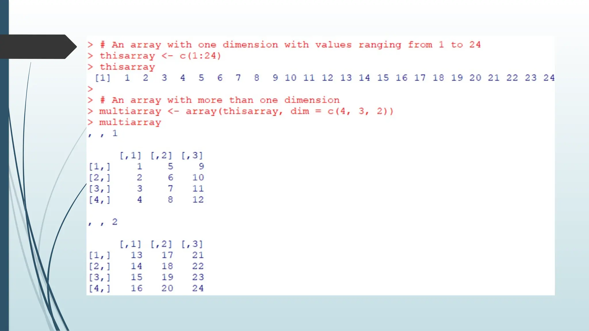
Arrays
Compared tomatrices, arrays can have more than two dimensions.
We can use the array() function to create an array, and the dim parameter to specify the
dimensions.
77.
Accessing Arrays
Youcan access the array elements by referring to the index position.
You can use the [] brackets to access the desired elements from an
array:
78.
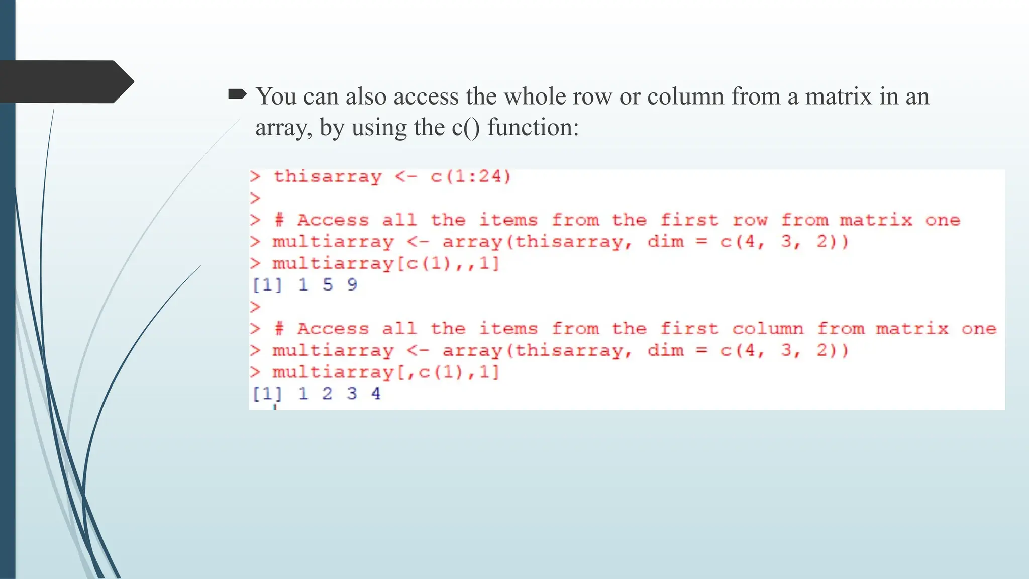
You canalso access the whole row or column from a matrix in an
array, by using the c() function:
79.
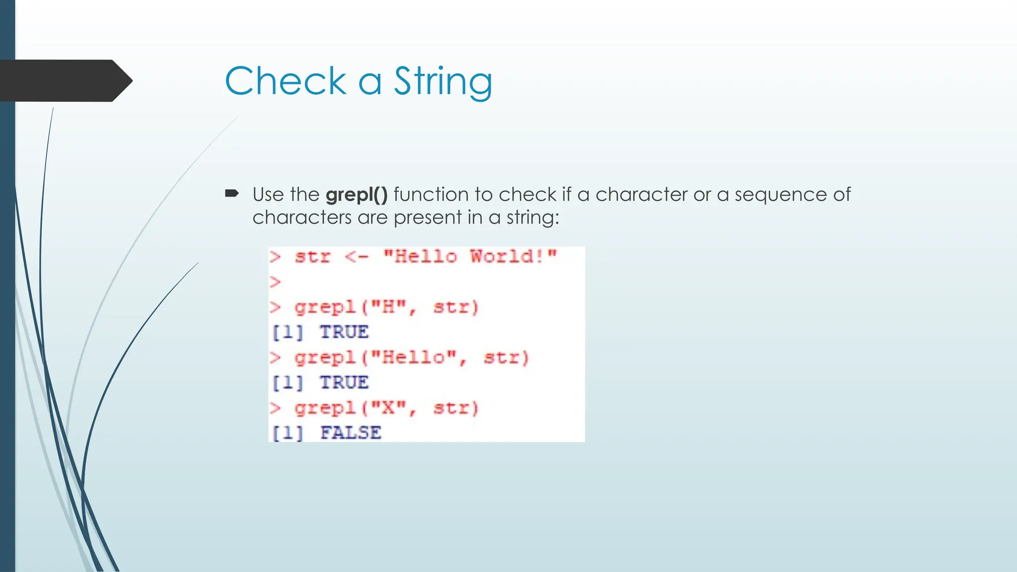
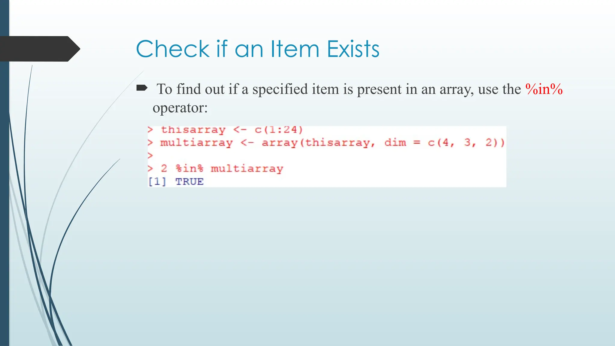
Check if anItem Exists
To find out if a specified item is present in an array, use the %in%
operator:
80.
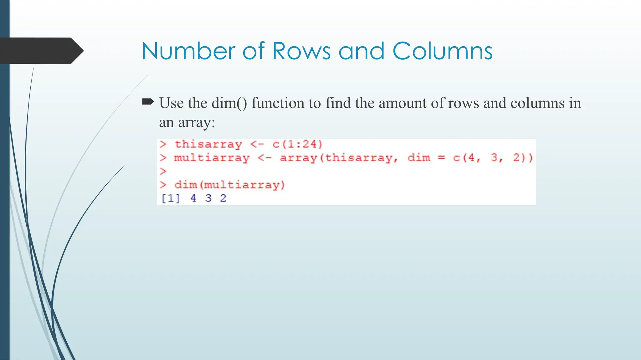
Number of Rowsand Columns
Use the dim() function to find the amount of rows and columns in
an array:
81.
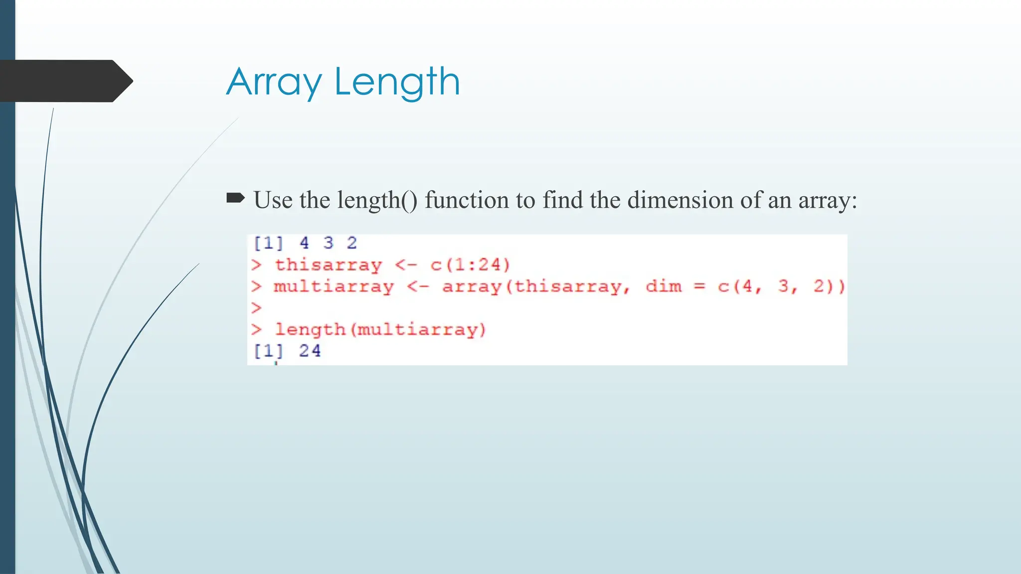
Array Length
Usethe length() function to find the dimension of an array:
R Data Frames
Data Frames are data displayed in a format as a table.
Data Frames can have different types of data inside it.
While the first column can be character, the second
and third can be numeric or logical. However, each
column should have the same type of data.
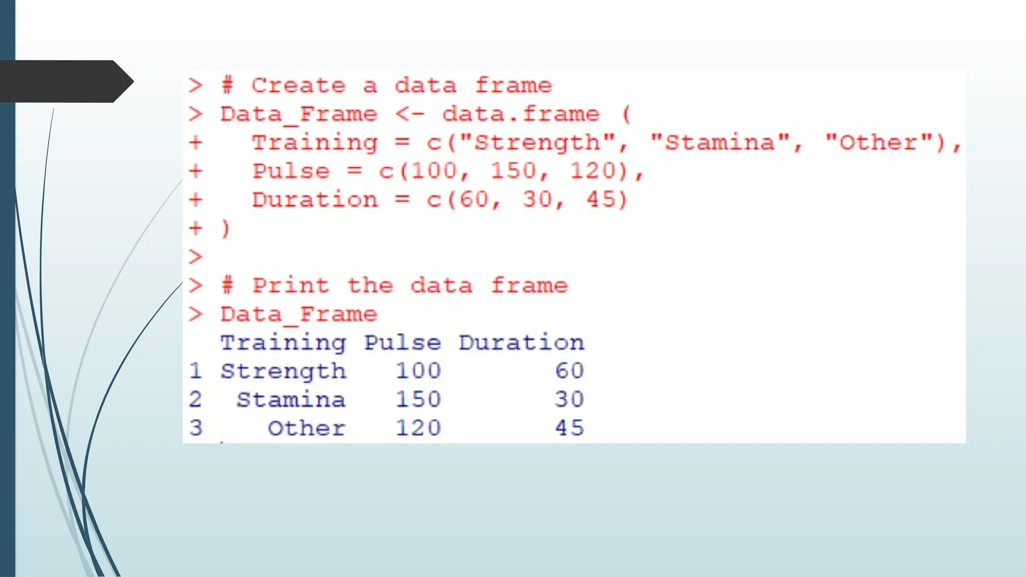
Use the data.frame() function to create a data frame:
85.
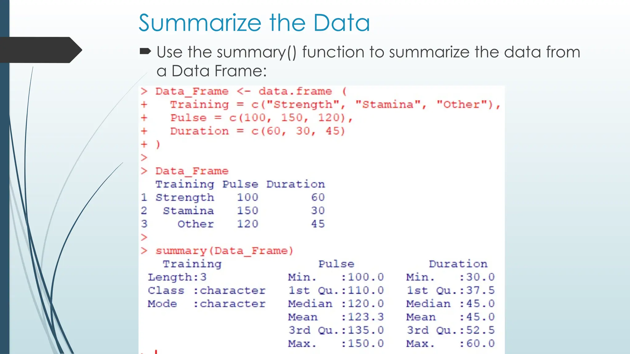
Summarize the Data
Use the summary() function to summarize the data from
a Data Frame:
86.
Access Items inFrames
We can use single brackets [ ], double brackets [[ ]] or $
to access columns from a data frame:
87.
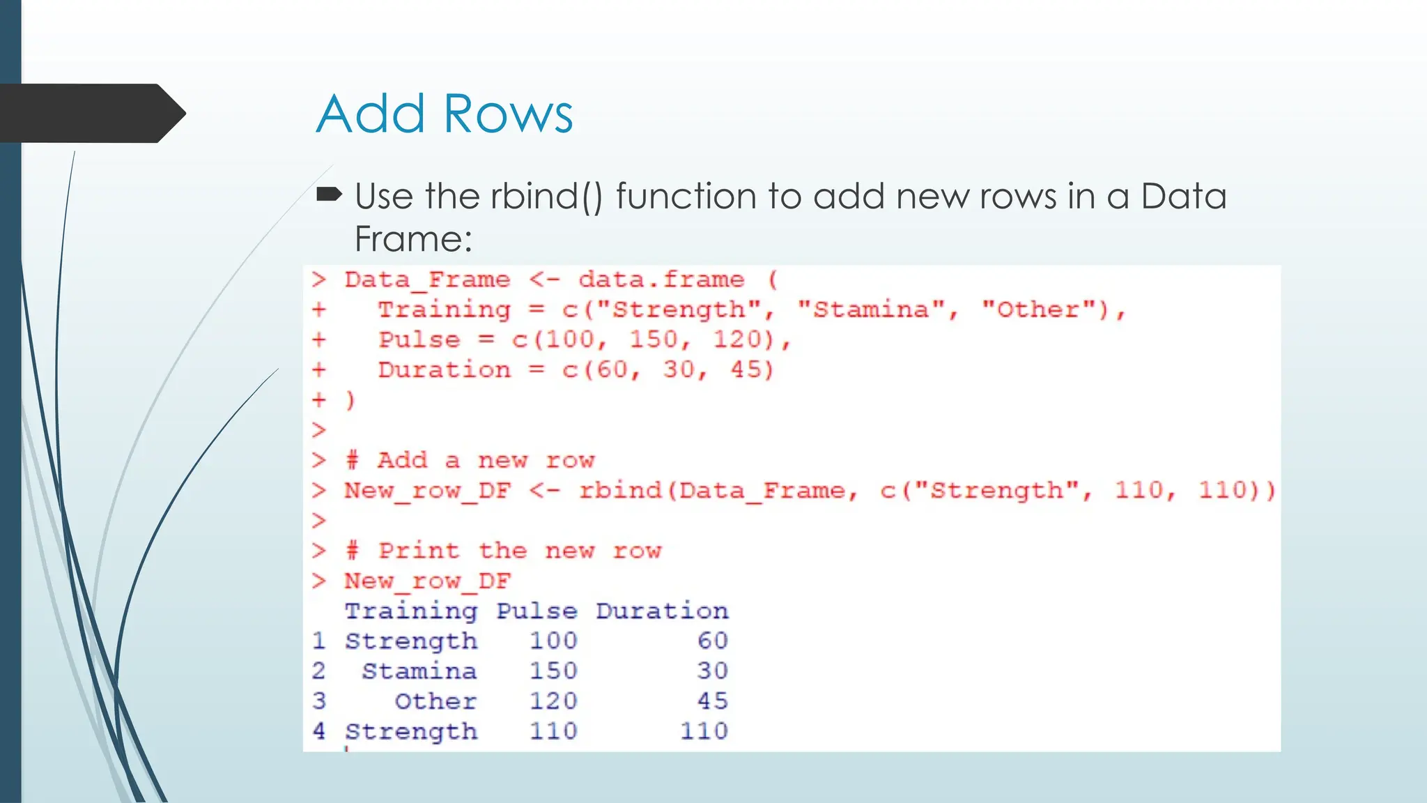
Add Rows
Usethe rbind() function to add new rows in a Data
Frame:
88.
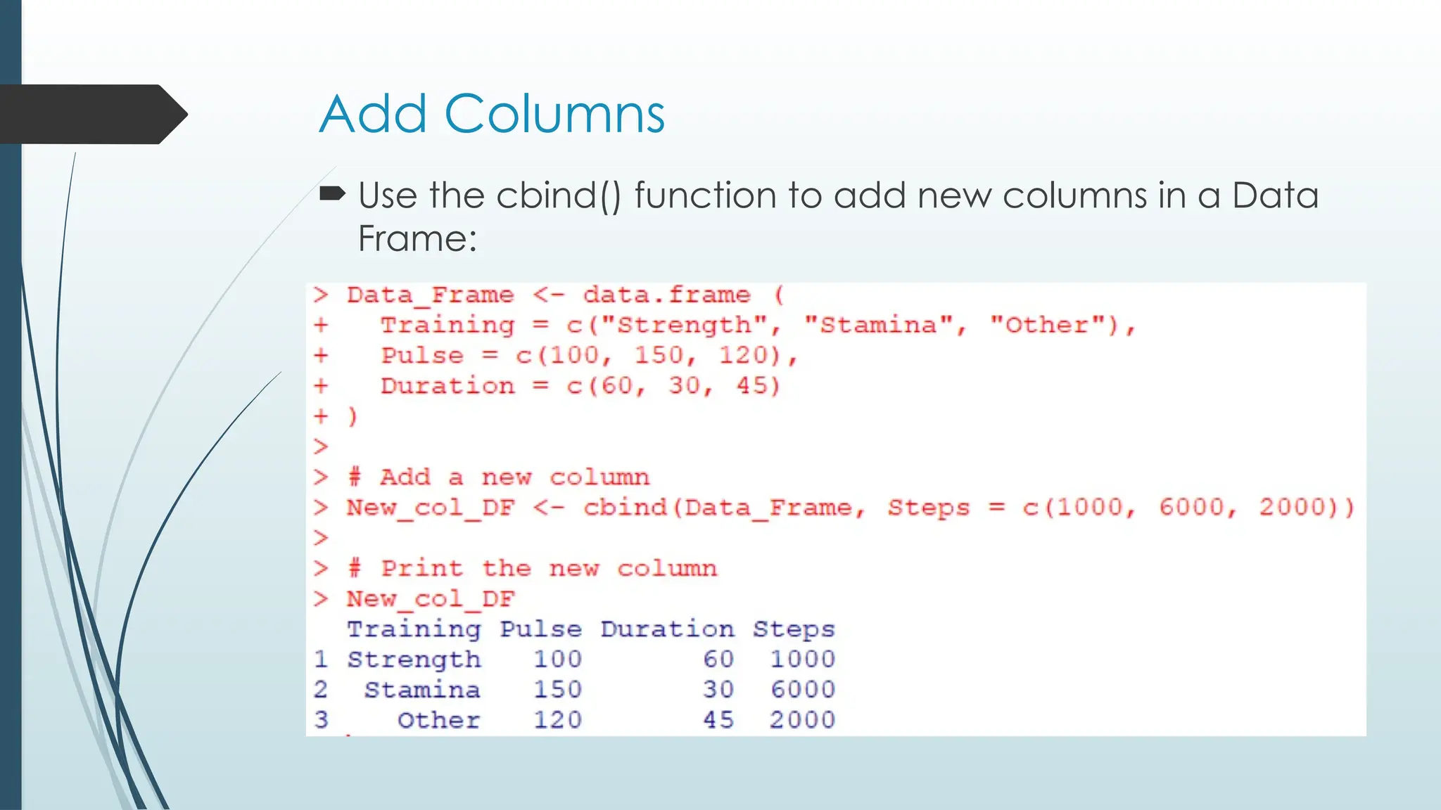
Add Columns
Usethe cbind() function to add new columns in a Data
Frame:
89.
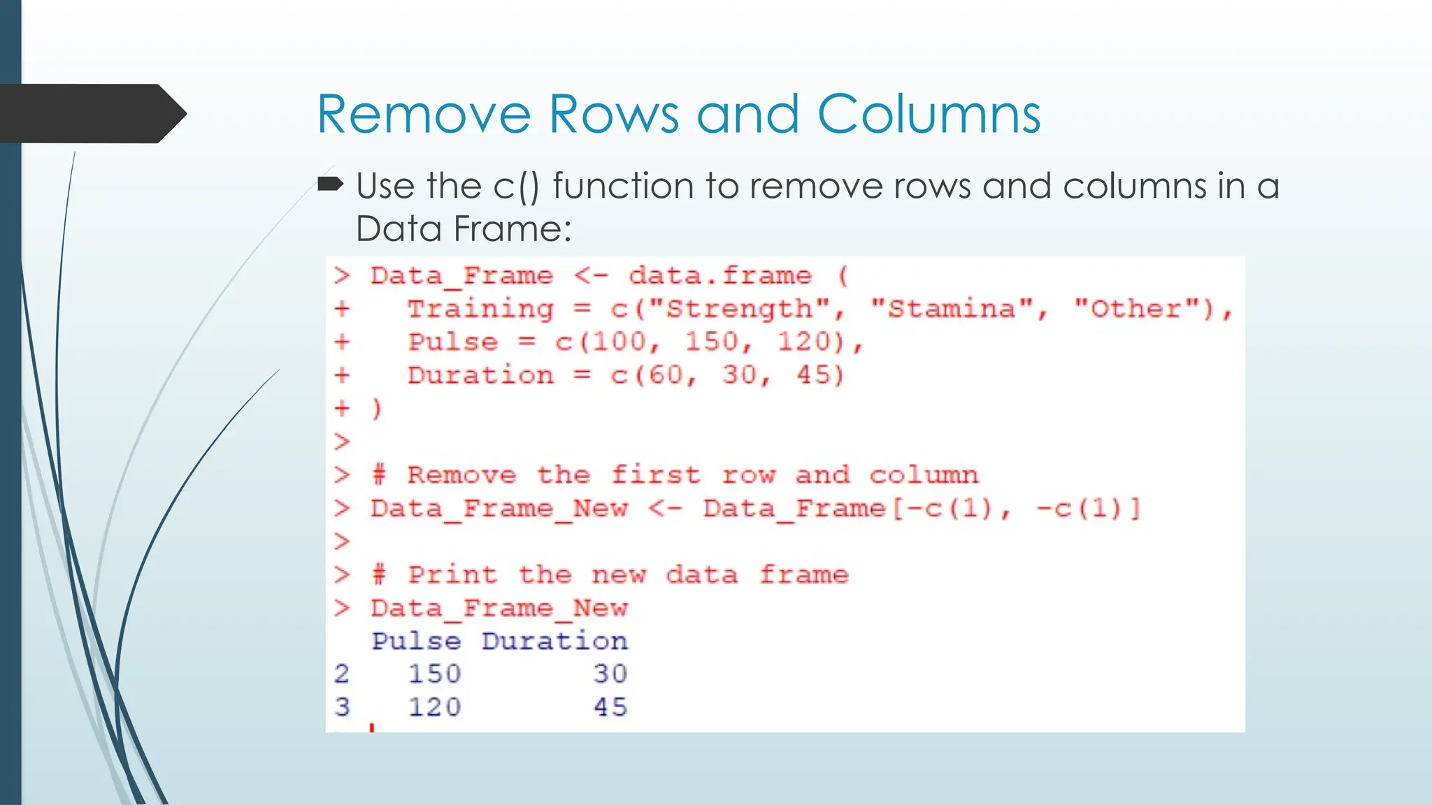
Remove Rows andColumns
Use the c() function to remove rows and columns in a
Data Frame:
90.
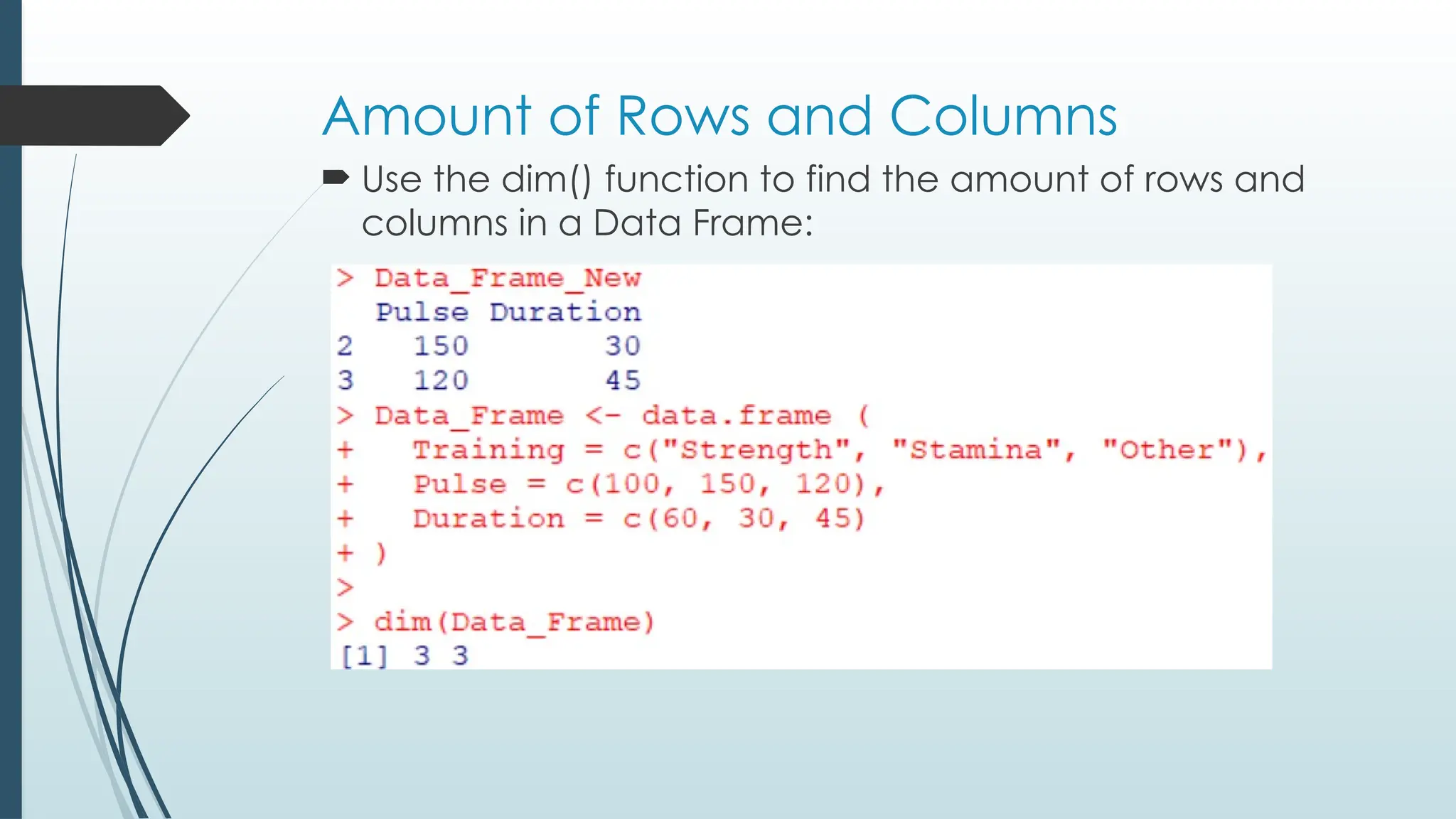
Amount of Rowsand Columns
Use the dim() function to find the amount of rows and
columns in a Data Frame:
91.
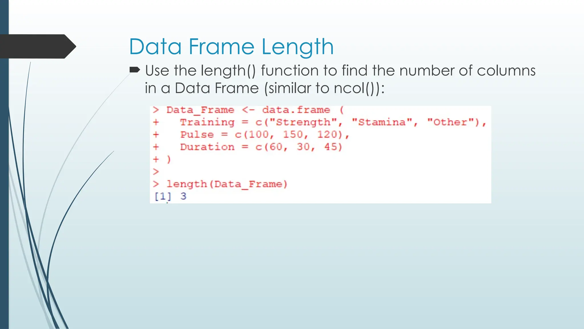
Data Frame Length
Use the length() function to find the number of columns
in a Data Frame (similar to ncol()):
92.
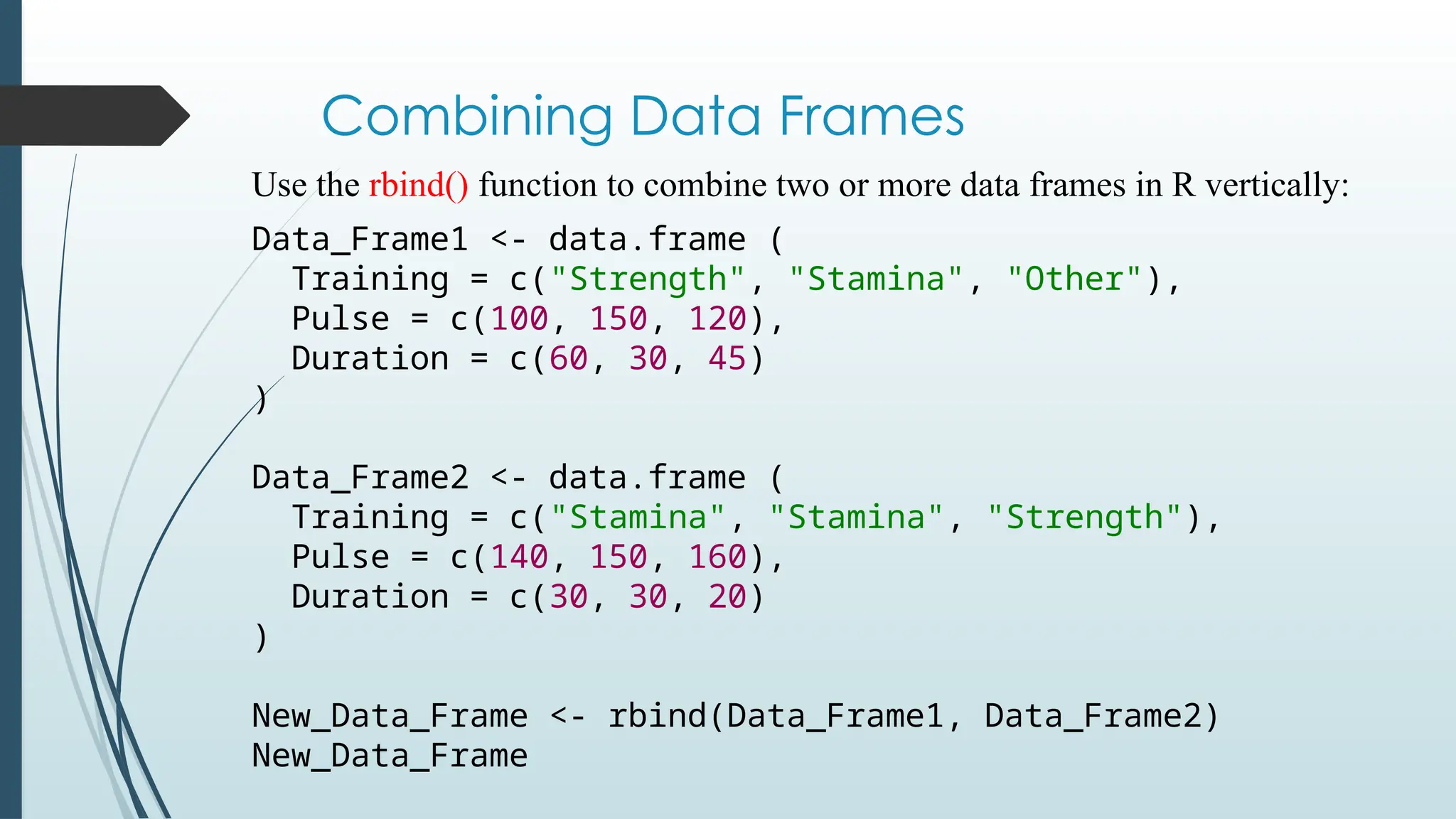
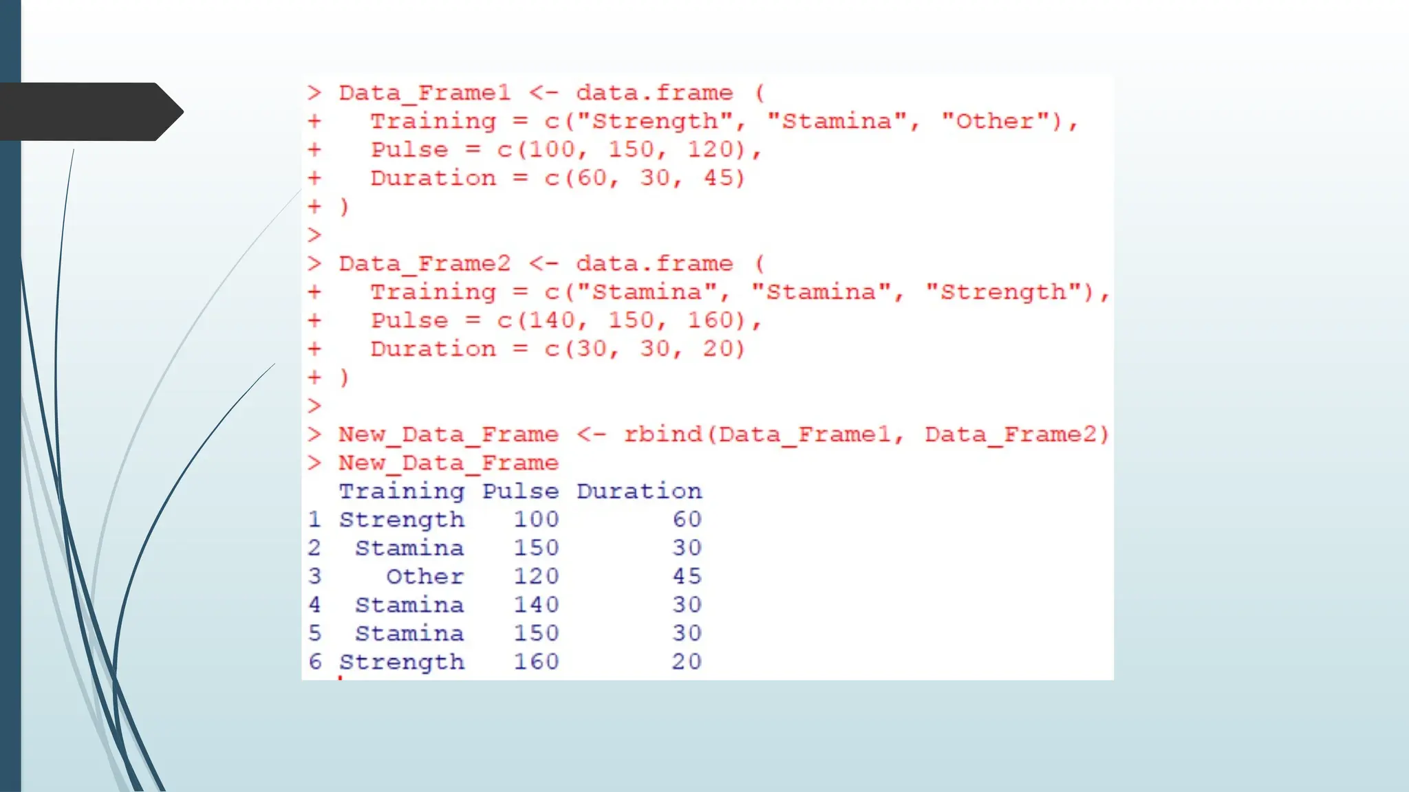
Combining Data Frames
Usethe rbind() function to combine two or more data frames in R vertically:
Data_Frame1 <- data.frame (
Training = c("Strength", "Stamina", "Other"),
Pulse = c(100, 150, 120),
Duration = c(60, 30, 45)
)
Data_Frame2 <- data.frame (
Training = c("Stamina", "Stamina", "Strength"),
Pulse = c(140, 150, 160),
Duration = c(30, 30, 20)
)
New_Data_Frame <- rbind(Data_Frame1, Data_Frame2)
New_Data_Frame
94.
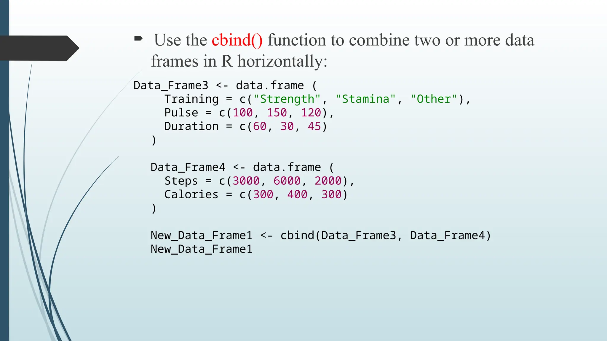
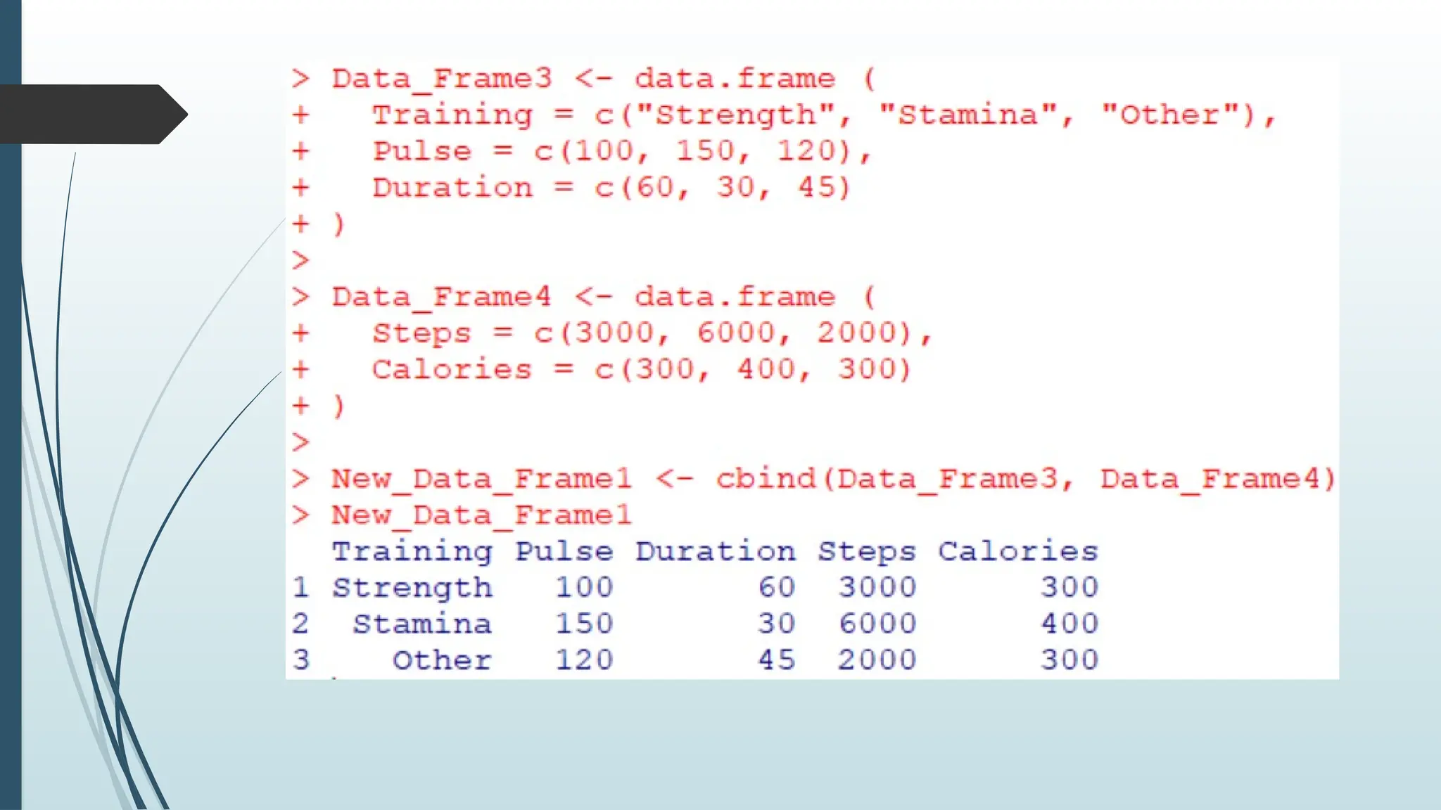
Use thecbind() function to combine two or more data
frames in R horizontally:
Data_Frame3 <- data.frame (
Training = c("Strength", "Stamina", "Other"),
Pulse = c(100, 150, 120),
Duration = c(60, 30, 45)
)
Data_Frame4 <- data.frame (
Steps = c(3000, 6000, 2000),
Calories = c(300, 400, 300)
)
New_Data_Frame1 <- cbind(Data_Frame3, Data_Frame4)
New_Data_Frame1
96.
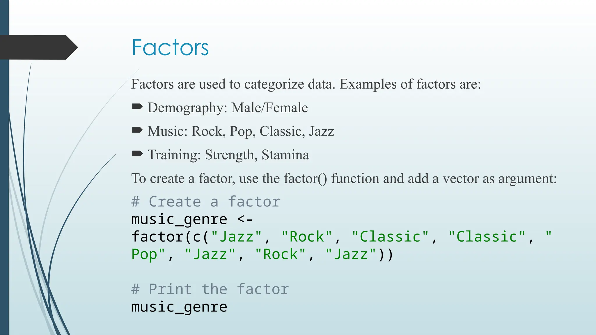
Factors
Factors are usedto categorize data. Examples of factors are:
Demography: Male/Female
Music: Rock, Pop, Classic, Jazz
Training: Strength, Stamina
To create a factor, use the factor() function and add a vector as argument:
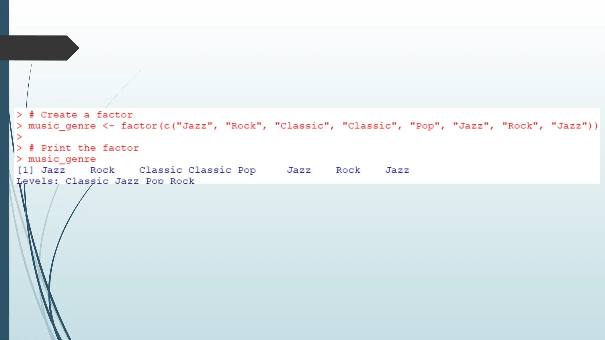
# Create a factor
music_genre <-
factor(c("Jazz", "Rock", "Classic", "Classic", "
Pop", "Jazz", "Rock", "Jazz"))
# Print the factor
music_genre
98.
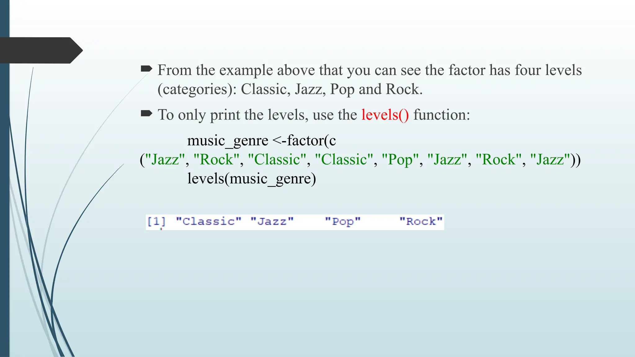
From theexample above that you can see the factor has four levels
(categories): Classic, Jazz, Pop and Rock.
To only print the levels, use the levels() function:
music_genre <-factor(c
("Jazz", "Rock", "Classic", "Classic", "Pop", "Jazz", "Rock", "Jazz"))
levels(music_genre)
99.
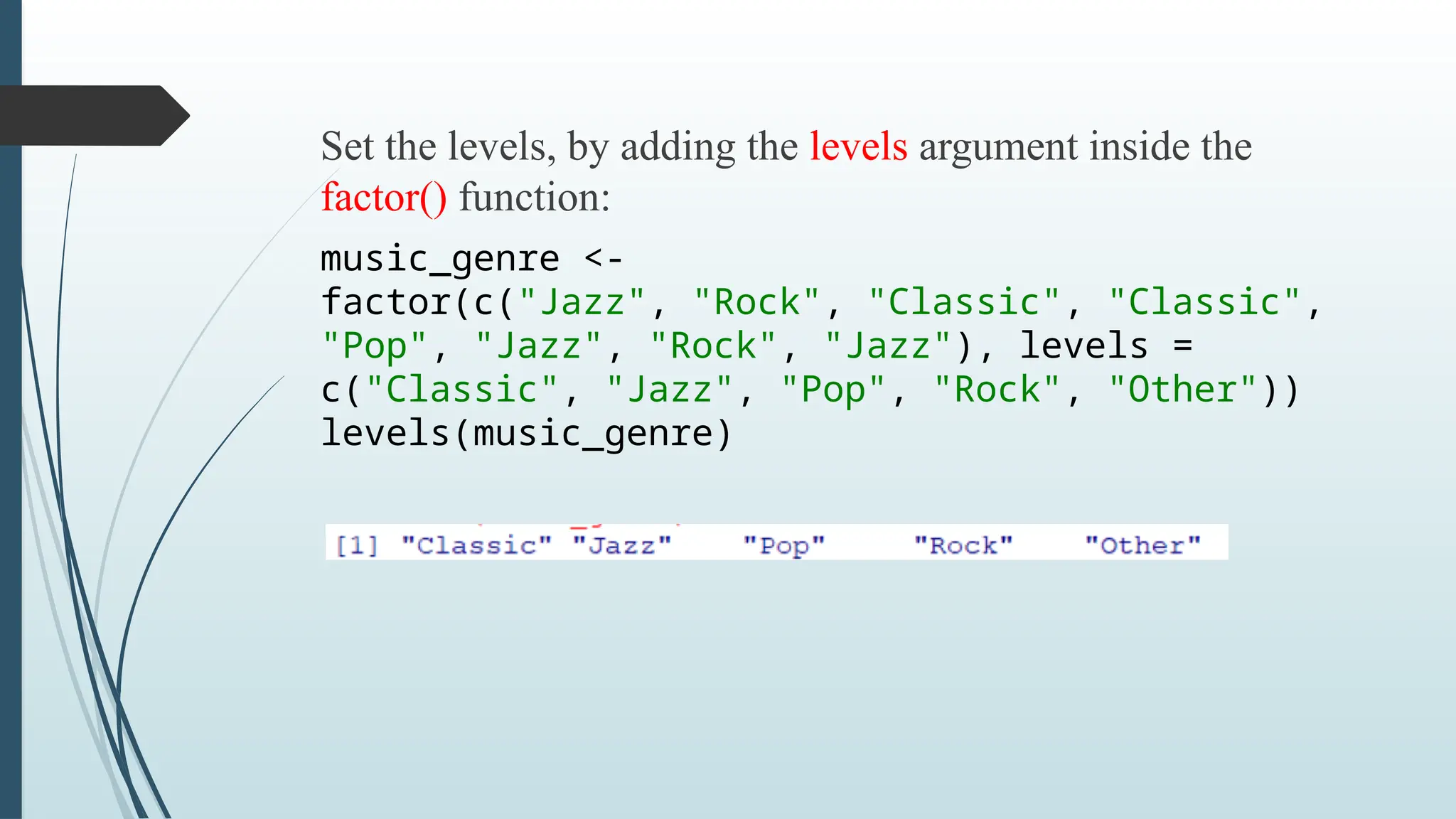
Set the levels,by adding the levels argument inside the
factor() function:
music_genre <-
factor(c("Jazz", "Rock", "Classic", "Classic",
"Pop", "Jazz", "Rock", "Jazz"), levels =
c("Classic", "Jazz", "Pop", "Rock", "Other"))
levels(music_genre)
100.
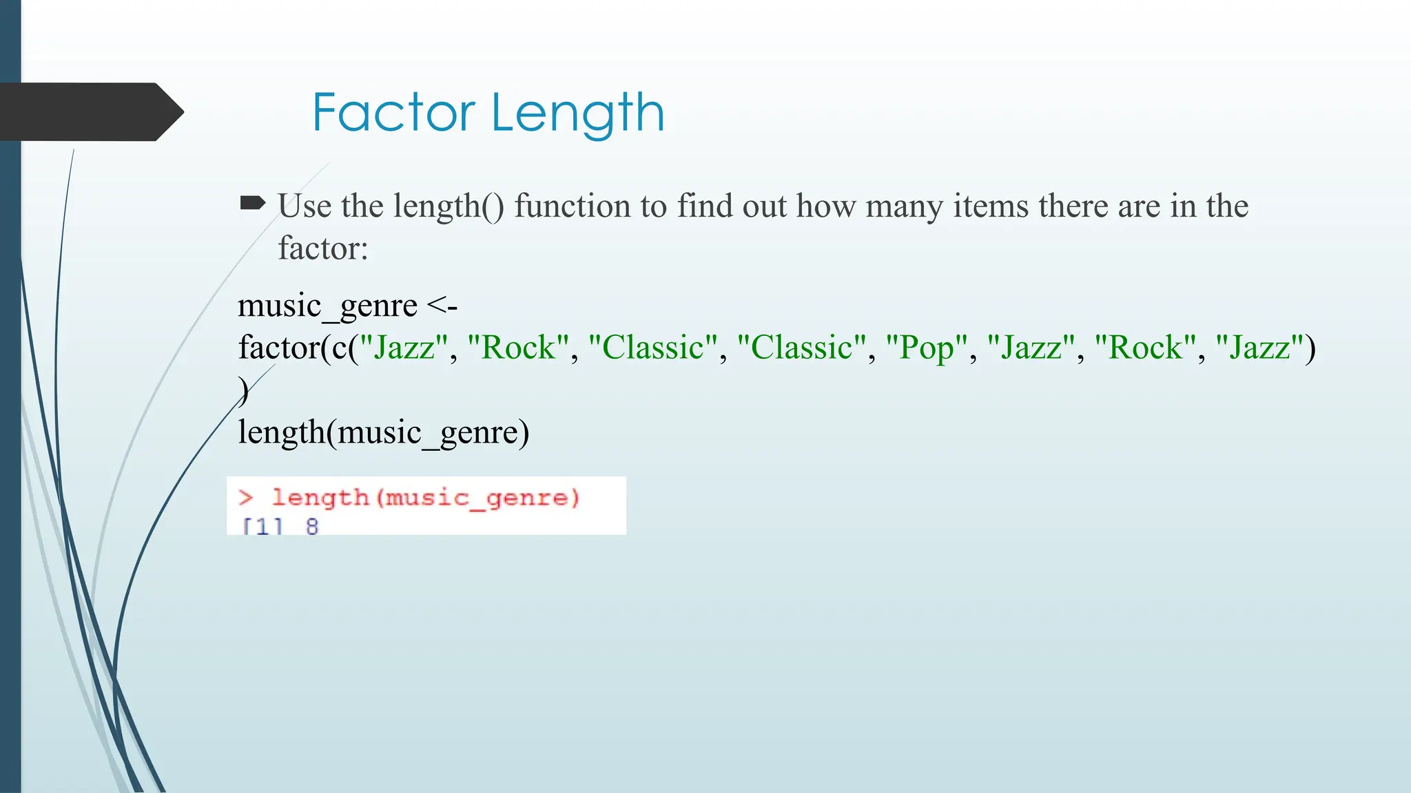
Factor Length
Usethe length() function to find out how many items there are in the
factor:
music_genre <-
factor(c("Jazz", "Rock", "Classic", "Classic", "Pop", "Jazz", "Rock", "Jazz")
)
length(music_genre)
101.
Access Factors
Toaccess the items in a factor, refer to the index number, using []
brackets:
102.
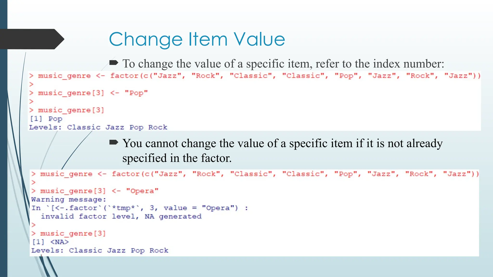
Change Item Value
To change the value of a specific item, refer to the index number:
You cannot change the value of a specific item if it is not already
specified in the factor.
103.
However, ifyou have already specified it inside the levels argument,
it will work:
music_genre <-
factor(c("Jazz", "Rock", "Classic", "Classic", "Pop", "Jazz", "Rock", "J
azz"), levels = c("Classic", "Jazz", "Pop", "Rock", "Opera"))
music_genre[3] <- "Opera"
music_genre[3]
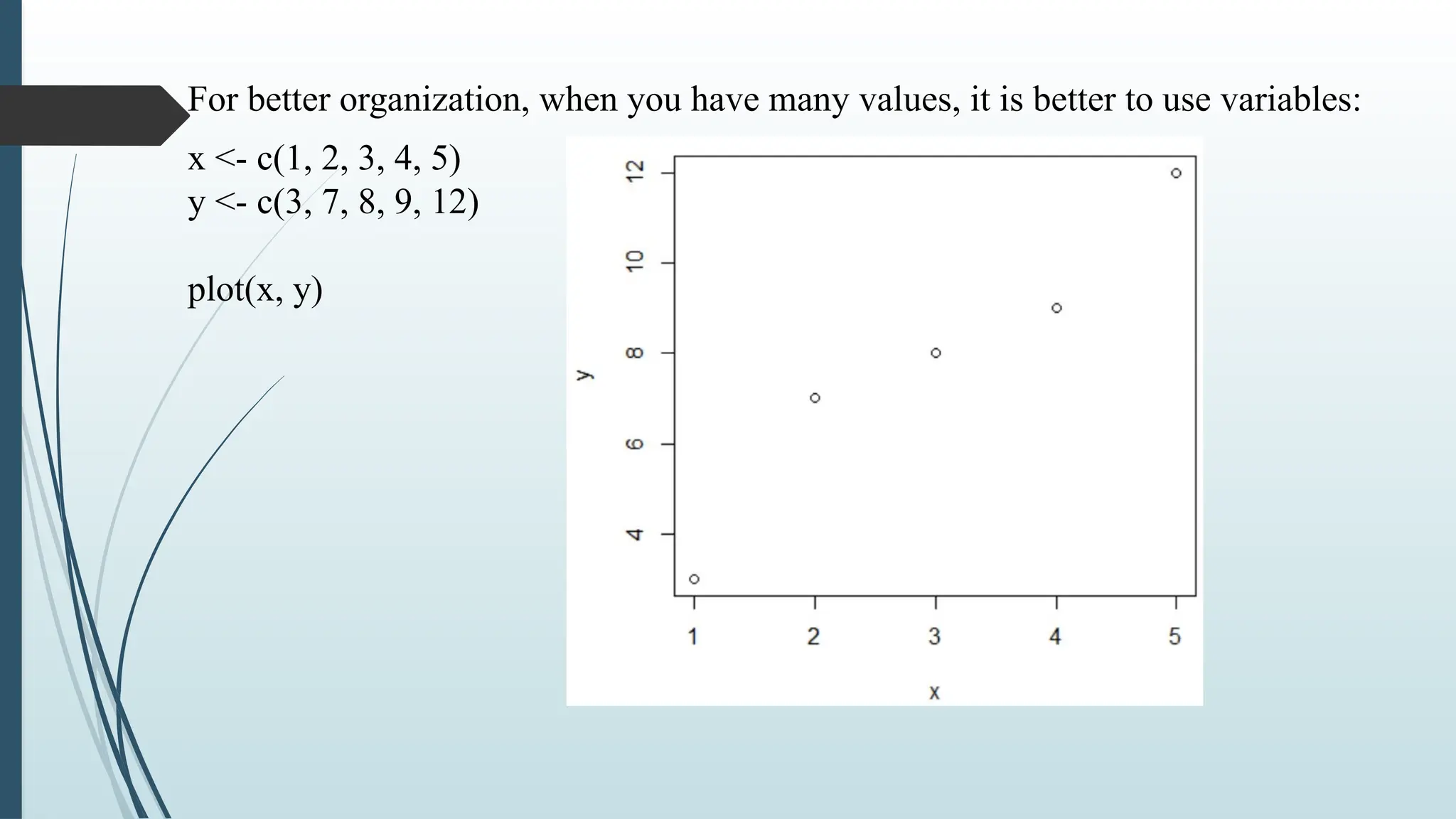
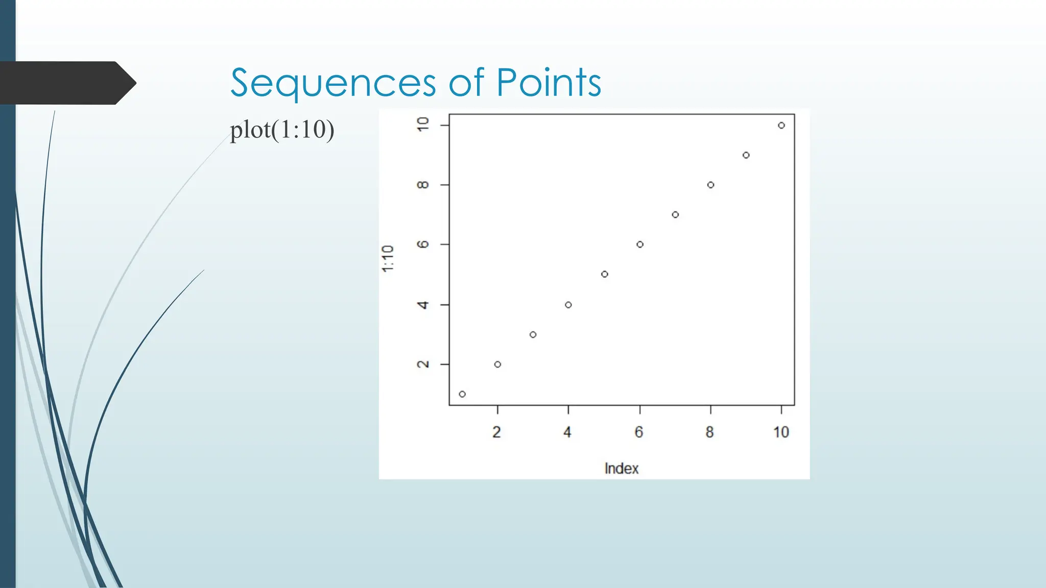
R Plotting
Theplot() function is used to draw points (markers) in a diagram.
The function takes parameters for specifying points in the diagram.
Parameter 1 specifies points on the x-axis.
Parameter 2 specifies points on the y-axis.
The plot() function to plot two numbers against each other:
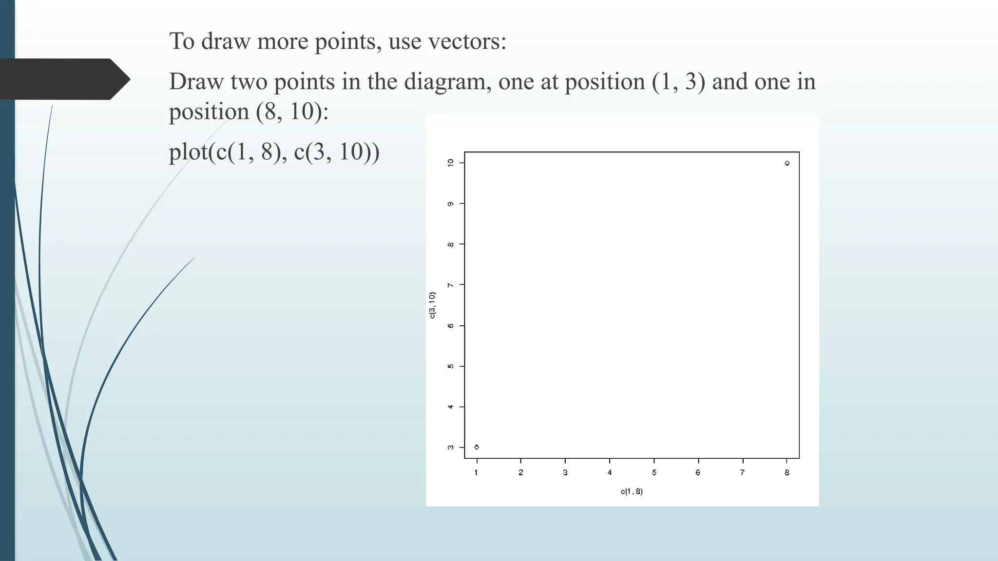
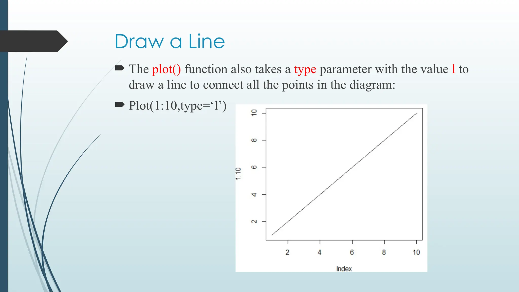
Draw a Line
The plot() function also takes a type parameter with the value l to
draw a line to connect all the points in the diagram:
Plot(1:10,type=‘l’)
112.
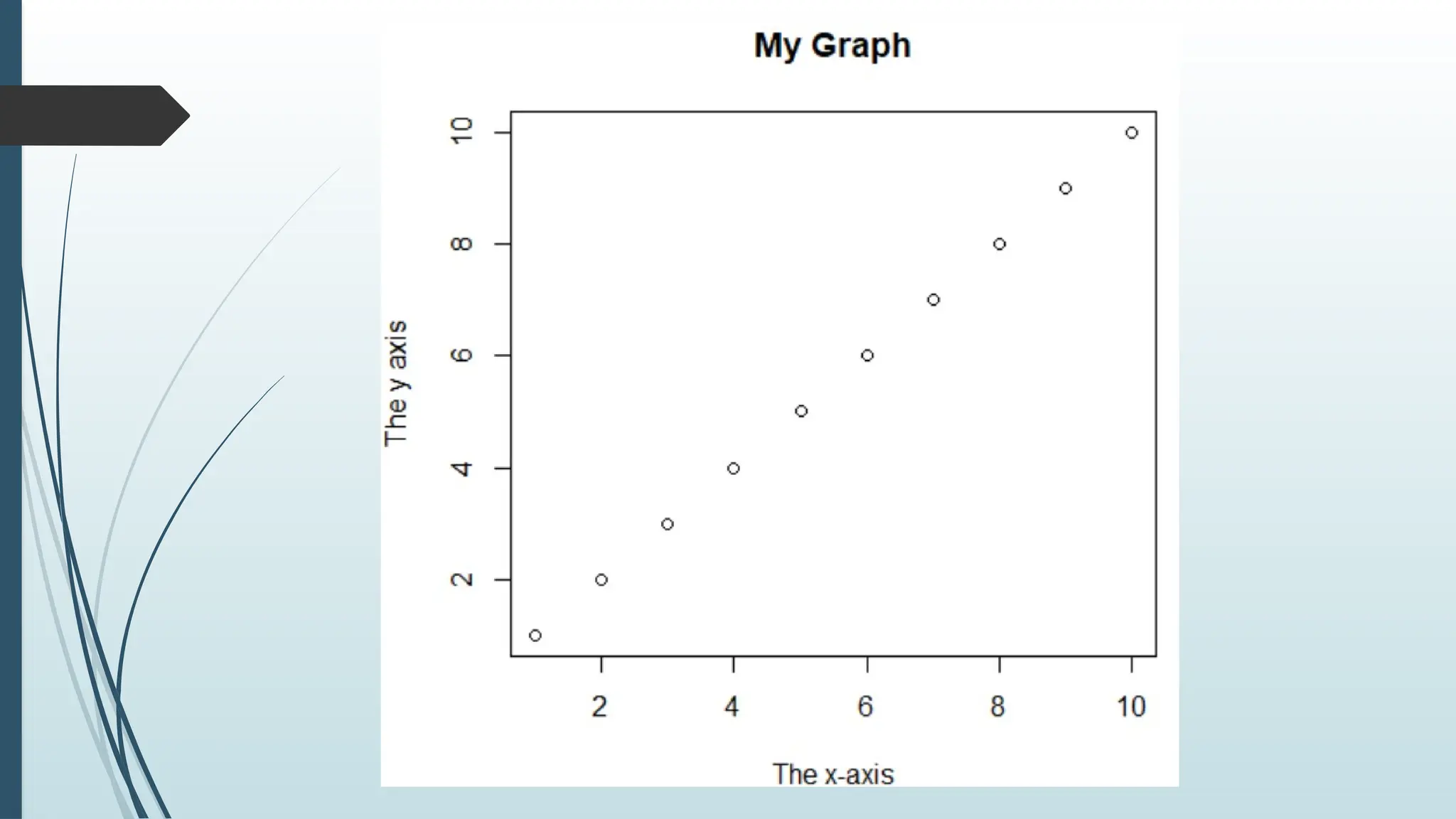
Plot Labels
The plot()function also accept other parameters, such as main, xlab
and ylab if you want to customize the graph with a main title and
different labels for the x and y-axis:
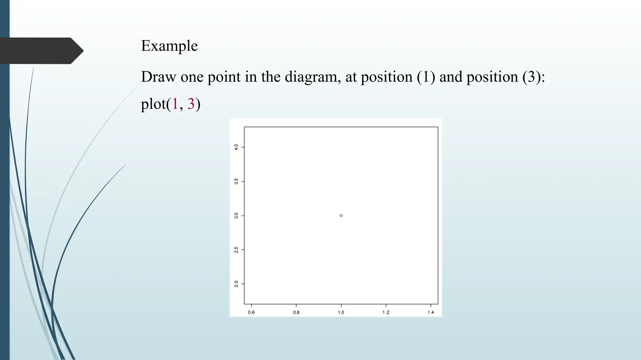
Example
plot(1:10, main="My Graph", xlab="The x-axis", ylab="The y axis")
114.
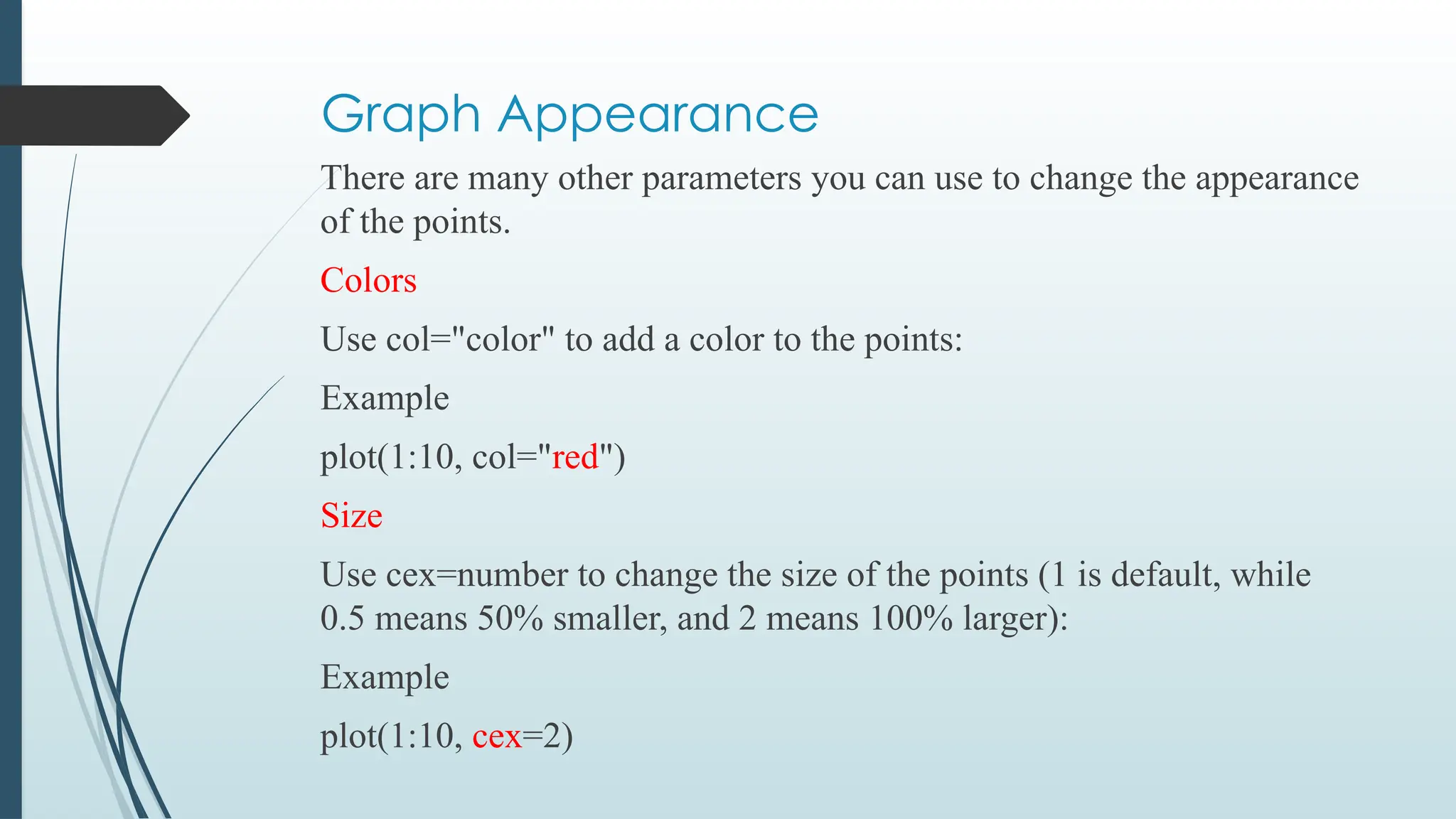
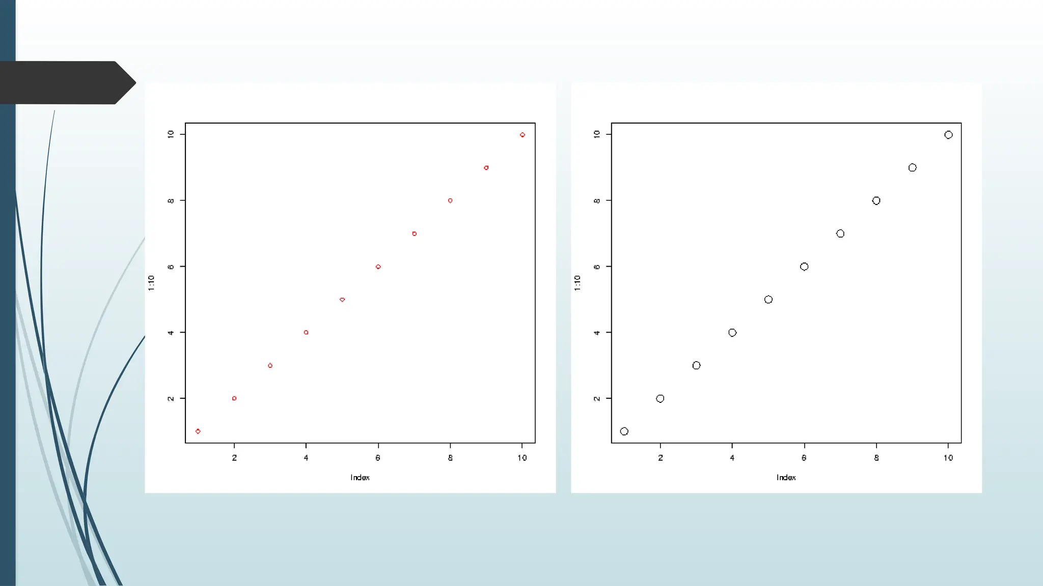
Graph Appearance
There aremany other parameters you can use to change the appearance
of the points.
Colors
Use col="color" to add a color to the points:
Example
plot(1:10, col="red")
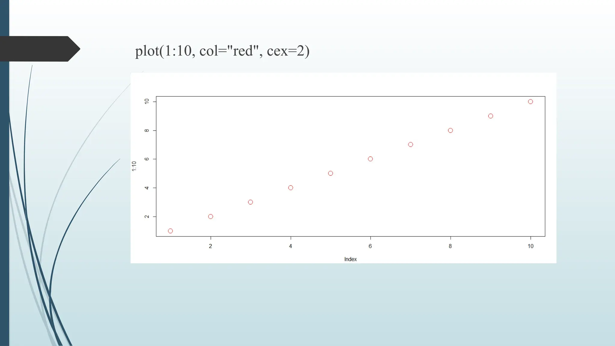
Size
Use cex=number to change the size of the points (1 is default, while
0.5 means 50% smaller, and 2 means 100% larger):
Example
plot(1:10, cex=2)
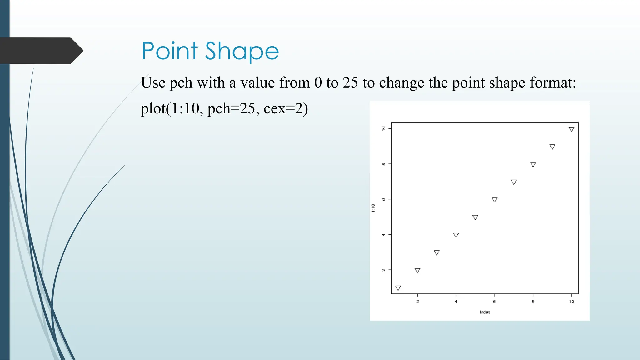
Point Shape
Use pchwith a value from 0 to 25 to change the point shape format:
plot(1:10, pch=25, cex=2)
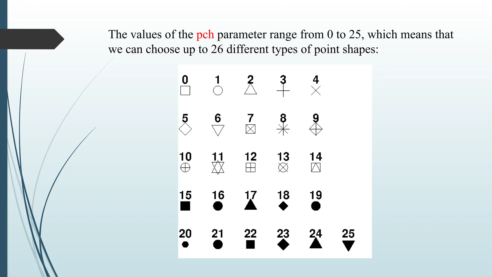
118.
The values ofthe pch parameter range from 0 to 25, which means that
we can choose up to 26 different types of point shapes:
119.
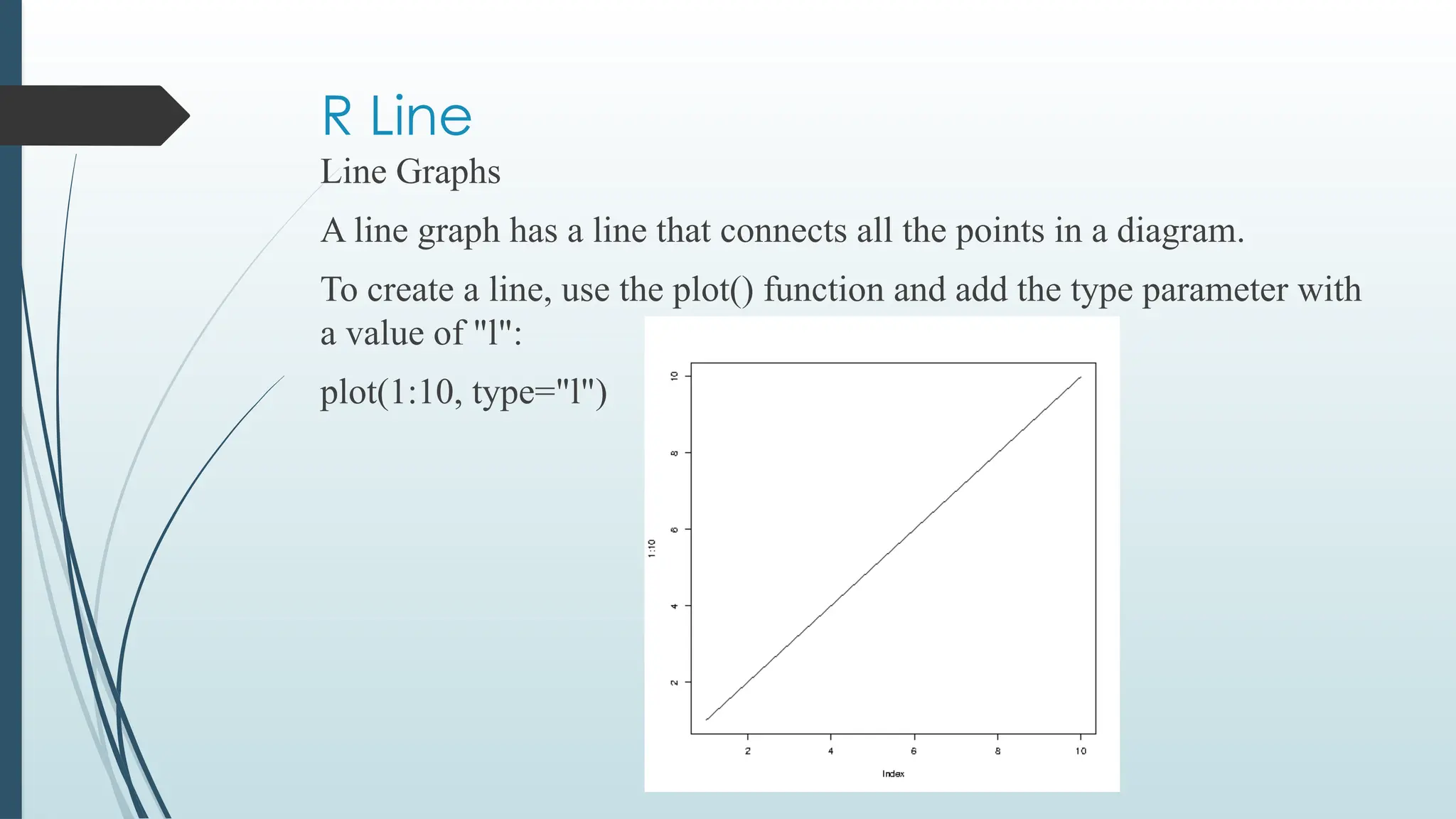
R Line
Line Graphs
Aline graph has a line that connects all the points in a diagram.
To create a line, use the plot() function and add the type parameter with
a value of "l":
plot(1:10, type="l")
120.
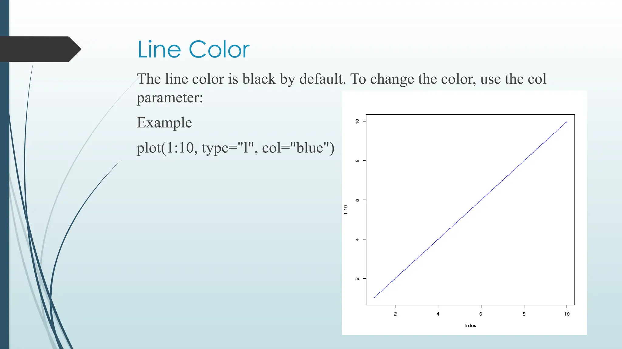
Line Color
The linecolor is black by default. To change the color, use the col
parameter:
Example
plot(1:10, type="l", col="blue")
121.
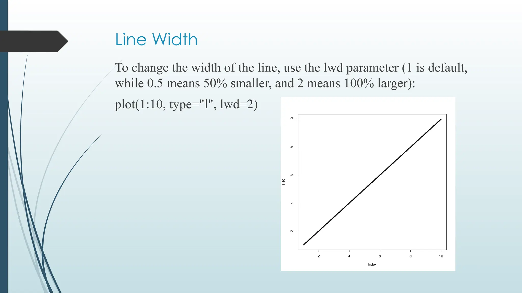
Line Width
To changethe width of the line, use the lwd parameter (1 is default,
while 0.5 means 50% smaller, and 2 means 100% larger):
plot(1:10, type="l", lwd=2)
122.
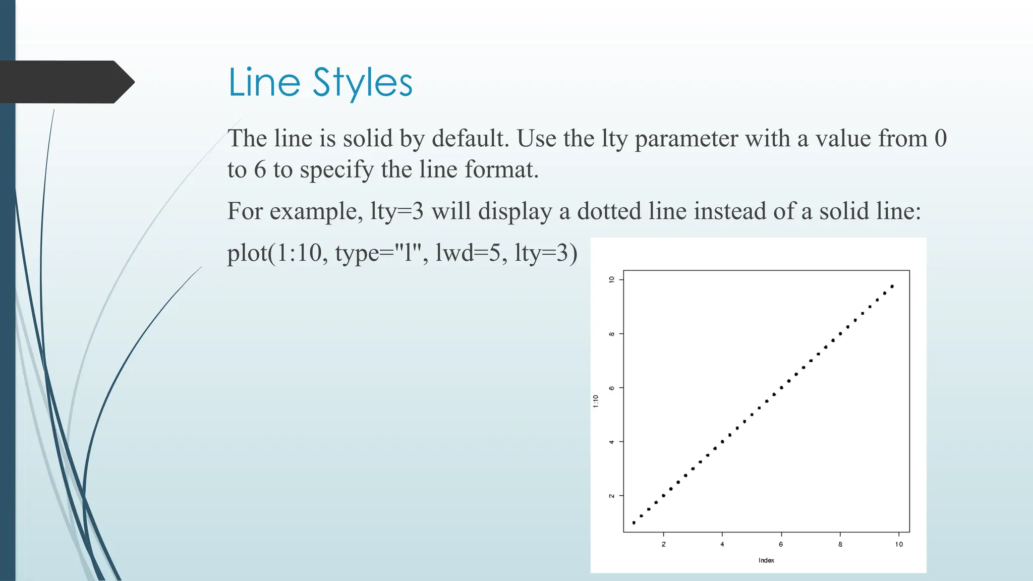
Line Styles
The lineis solid by default. Use the lty parameter with a value from 0
to 6 to specify the line format.
For example, lty=3 will display a dotted line instead of a solid line:
plot(1:10, type="l", lwd=5, lty=3)
123.
Available parameter valuesfor lty:
• 0 removes the line
• 1 displays a solid line
• 2 displays a dashed line
• 3 displays a dotted line
• 4 displays a "dot dashed" line
• 5 displays a "long dashed" line
• 6 displays a "two dashed" line
124.
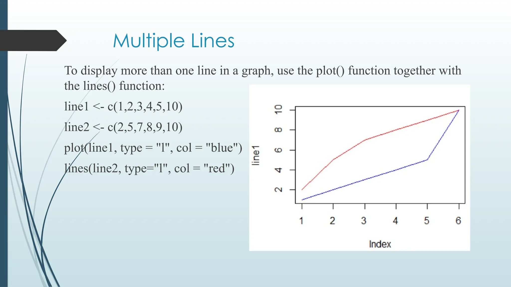
Multiple Lines
To displaymore than one line in a graph, use the plot() function together with
the lines() function:
line1 <- c(1,2,3,4,5,10)
line2 <- c(2,5,7,8,9,10)
plot(line1, type = "l", col = "blue")
lines(line2, type="l", col = "red")
125.
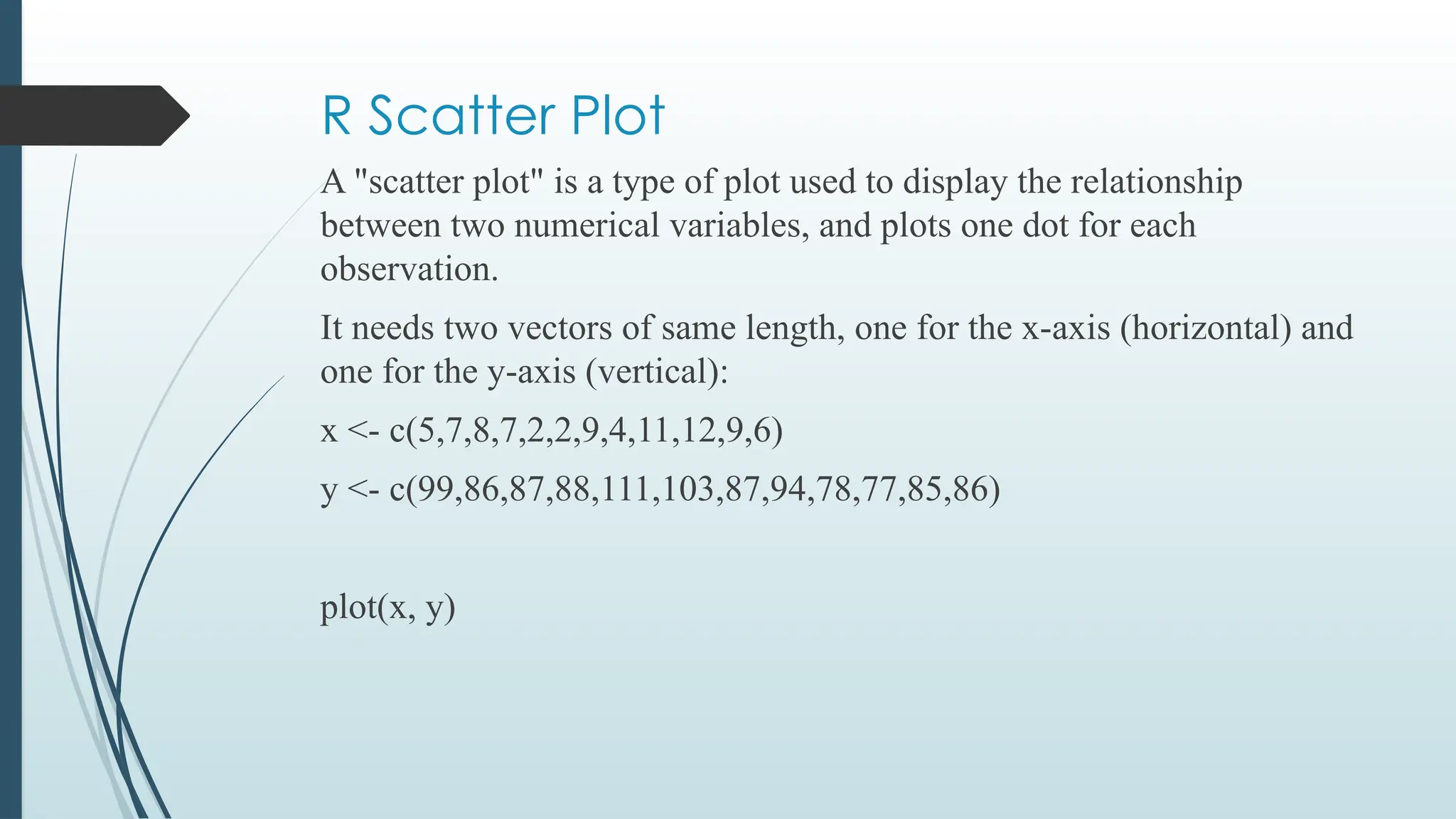
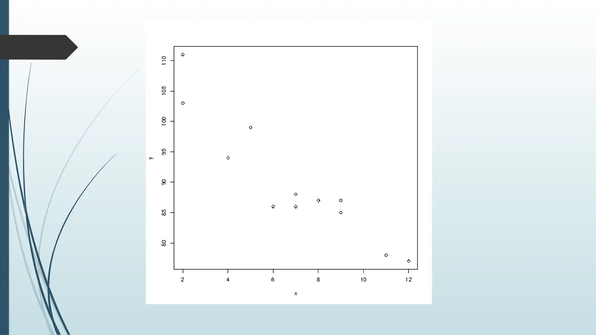
R Scatter Plot
A"scatter plot" is a type of plot used to display the relationship
between two numerical variables, and plots one dot for each
observation.
It needs two vectors of same length, one for the x-axis (horizontal) and
one for the y-axis (vertical):
x <- c(5,7,8,7,2,2,9,4,11,12,9,6)
y <- c(99,86,87,88,111,103,87,94,78,77,85,86)
plot(x, y)
127.
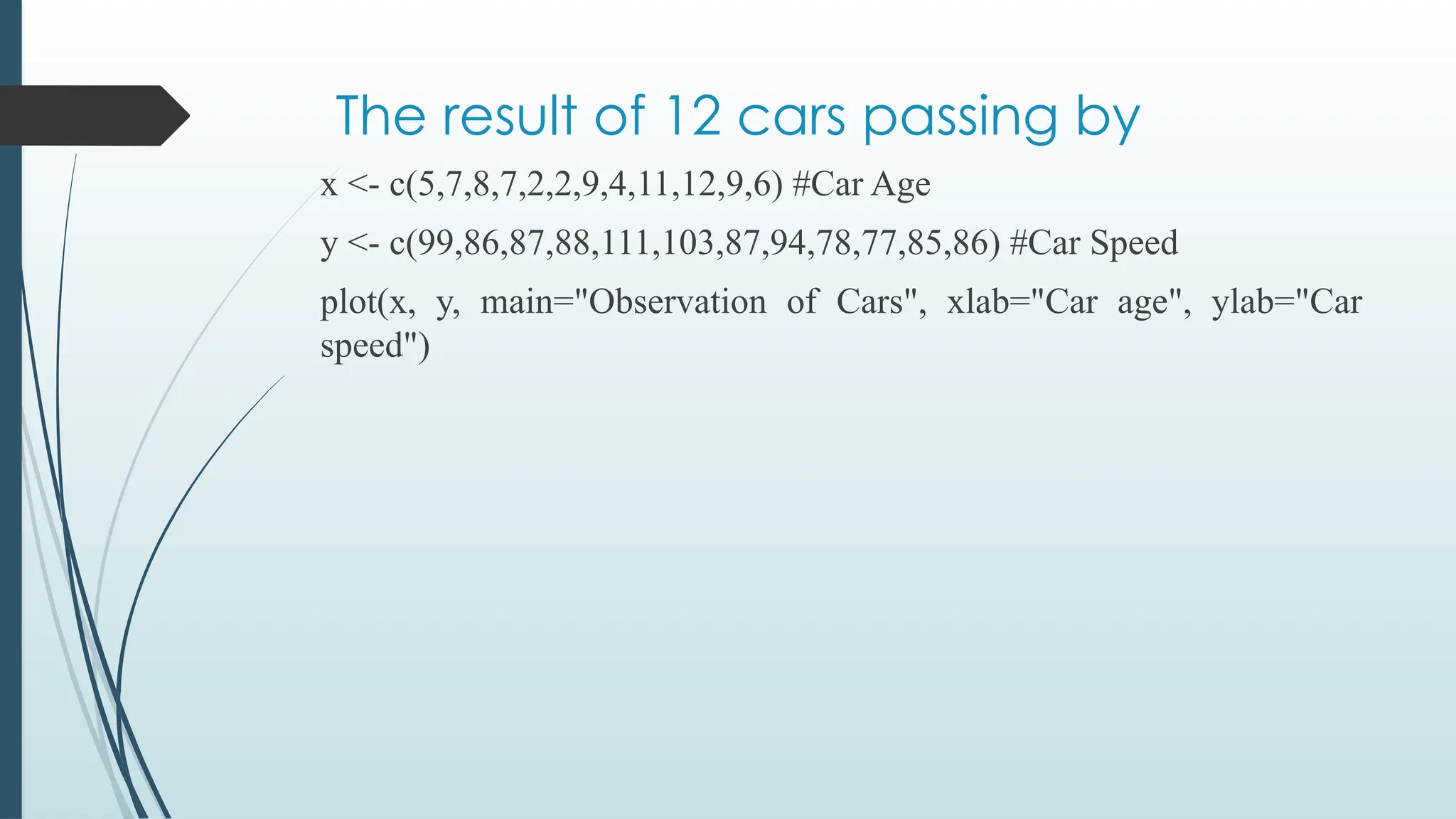
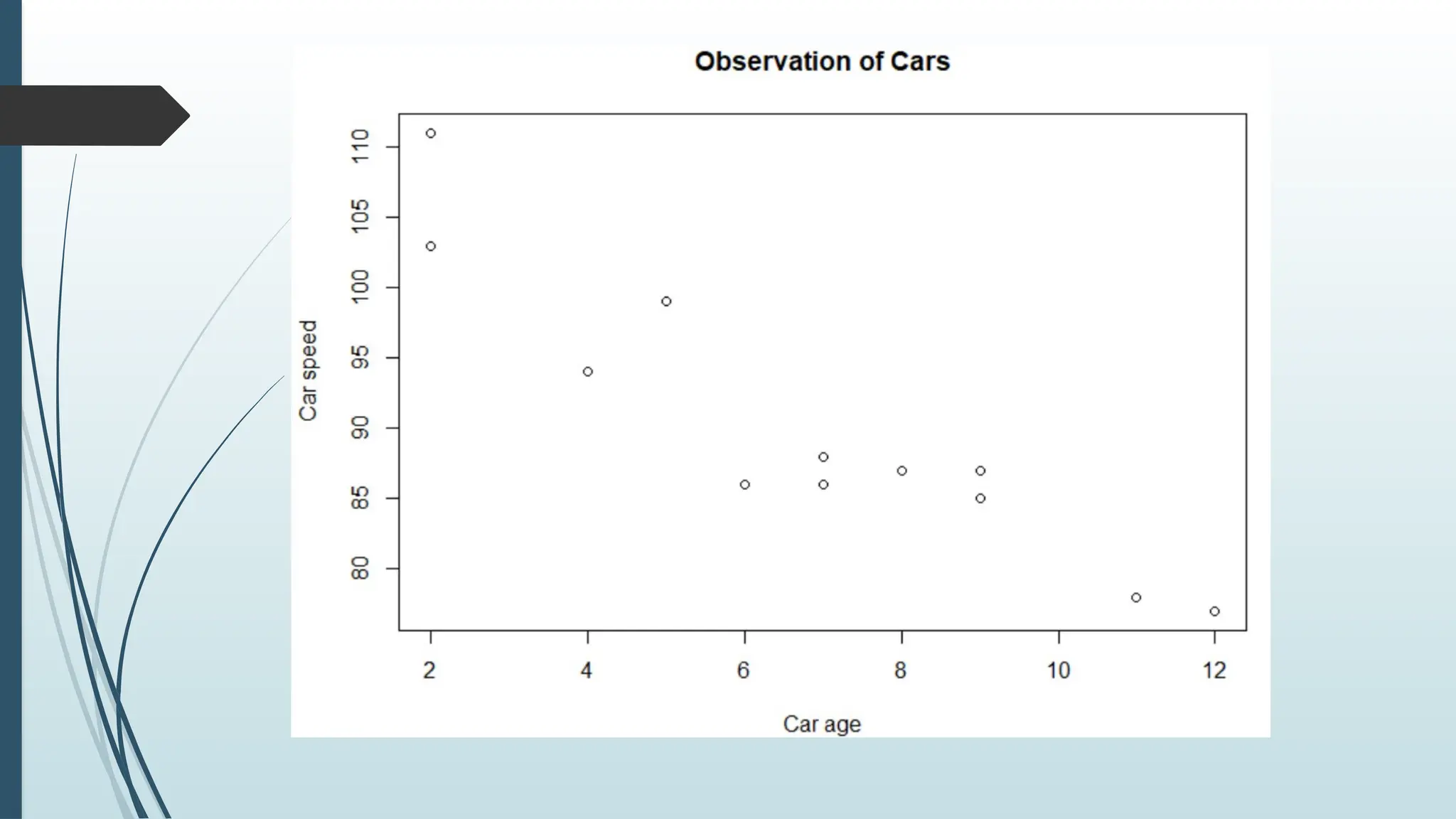
x <- c(5,7,8,7,2,2,9,4,11,12,9,6)#Car Age
y <- c(99,86,87,88,111,103,87,94,78,77,85,86) #Car Speed
plot(x, y, main="Observation of Cars", xlab="Car age", ylab="Car
speed")
The result of 12 cars passing by
129.
Inferences
The x-axisshows how old the car is.
The y-axis shows the speed of the car when it passes.
Are there any relationships between the observations?
It seems that the newer the car, the faster it drives, but that could be
a coincidence, after all we only registered 12 cars.
130.
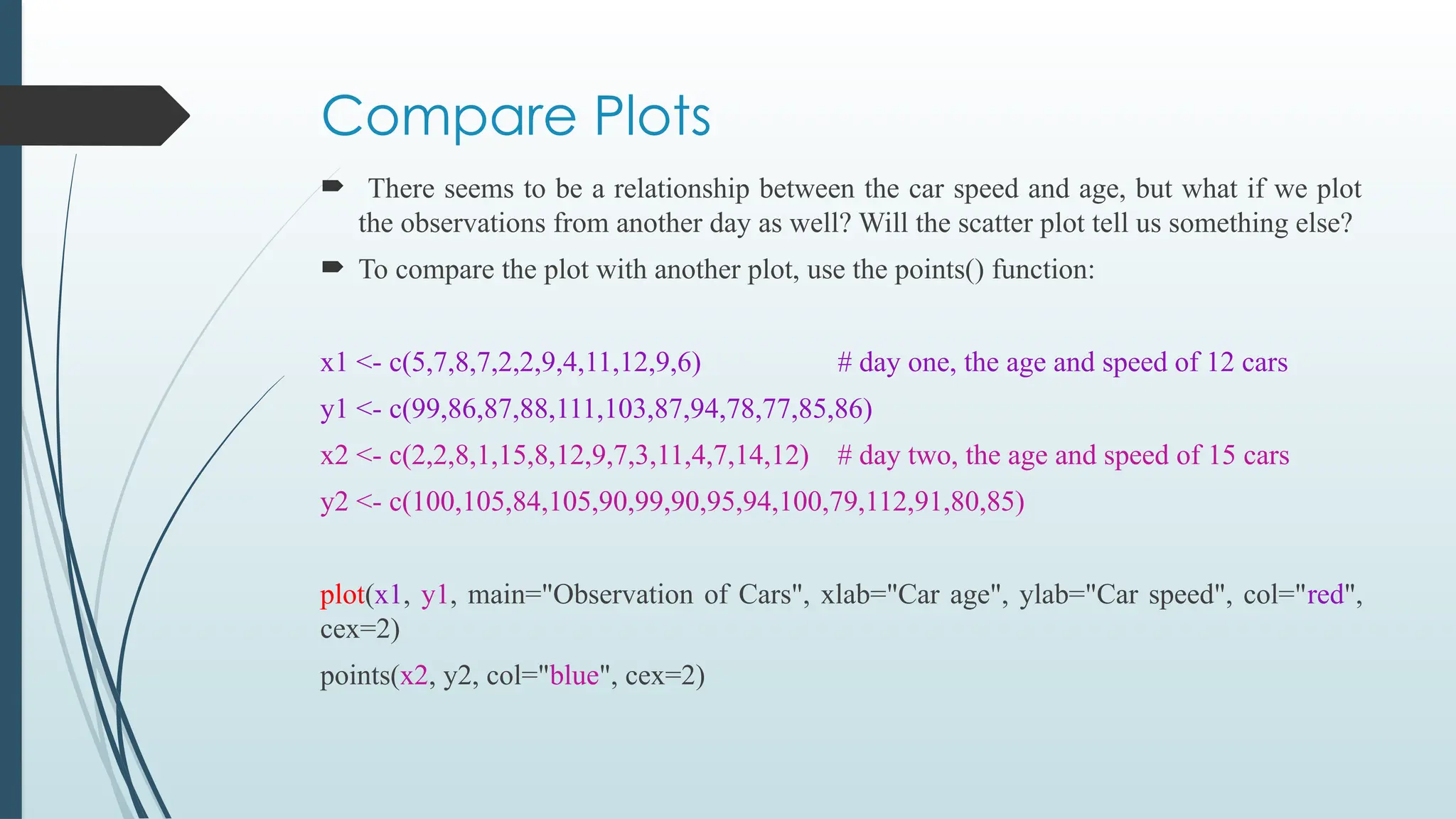
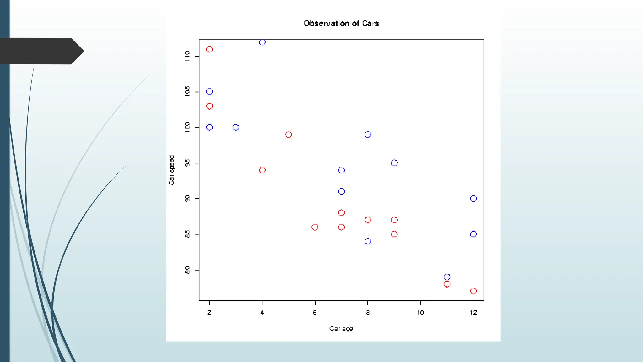
Compare Plots
Thereseems to be a relationship between the car speed and age, but what if we plot
the observations from another day as well? Will the scatter plot tell us something else?
To compare the plot with another plot, use the points() function:
x1 <- c(5,7,8,7,2,2,9,4,11,12,9,6) # day one, the age and speed of 12 cars
y1 <- c(99,86,87,88,111,103,87,94,78,77,85,86)
x2 <- c(2,2,8,1,15,8,12,9,7,3,11,4,7,14,12) # day two, the age and speed of 15 cars
y2 <- c(100,105,84,105,90,99,90,95,94,100,79,112,91,80,85)
plot(x1, y1, main="Observation of Cars", xlab="Car age", ylab="Car speed", col="red",
cex=2)
points(x2, y2, col="blue", cex=2)
132.
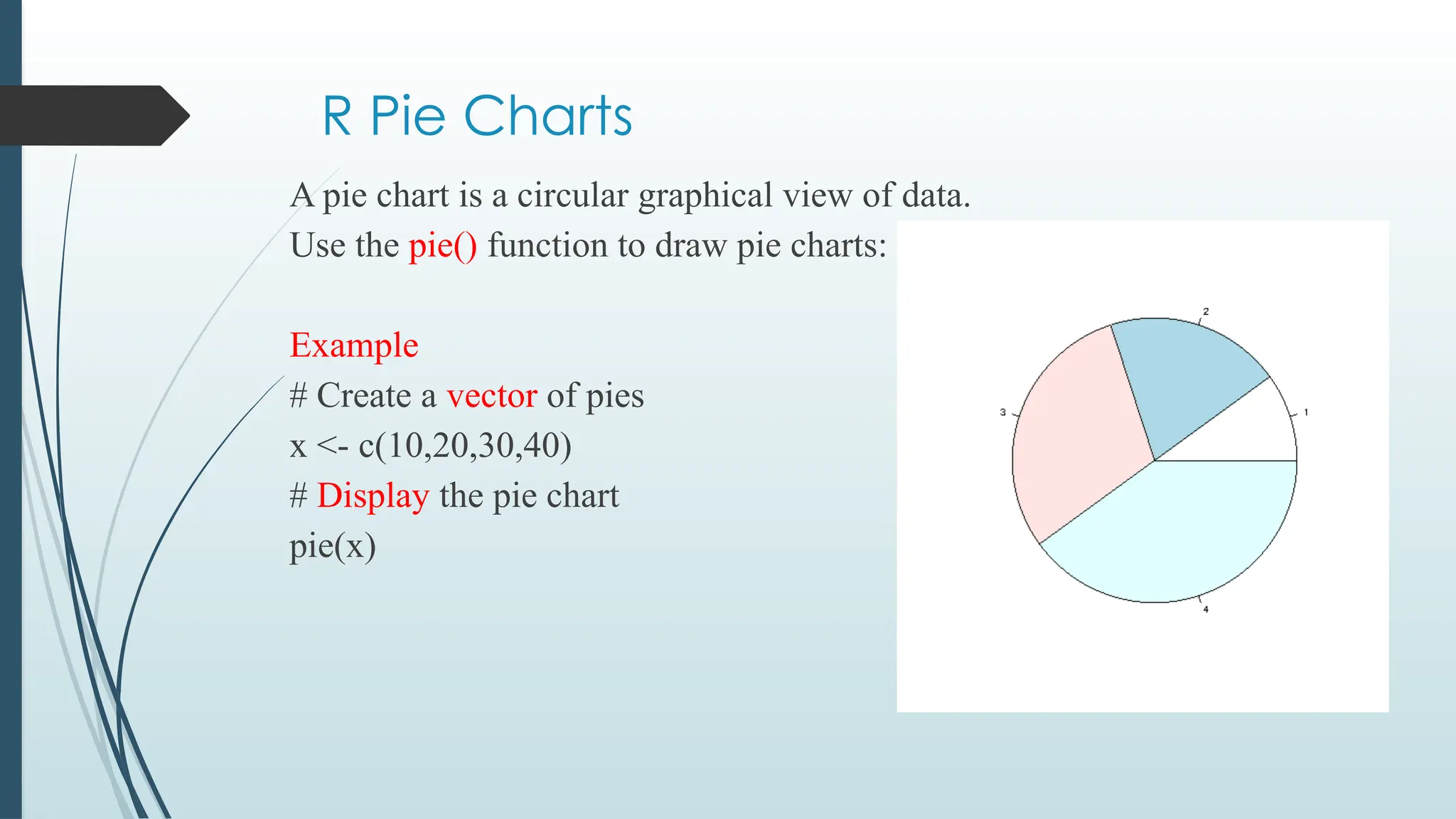
R Pie Charts
Apie chart is a circular graphical view of data.
Use the pie() function to draw pie charts:
Example
# Create a vector of pies
x <- c(10,20,30,40)
# Display the pie chart
pie(x)
133.
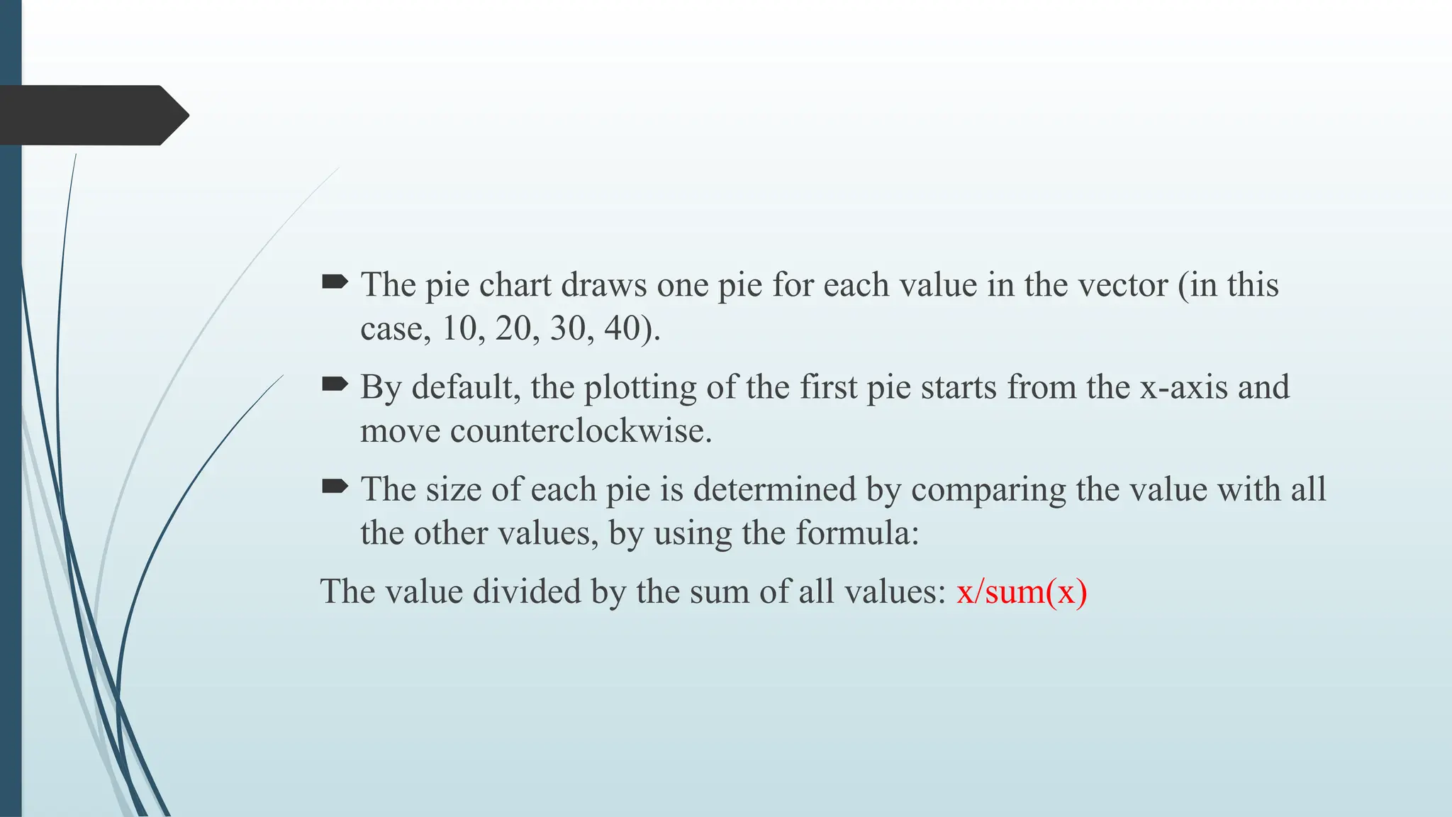
The piechart draws one pie for each value in the vector (in this
case, 10, 20, 30, 40).
By default, the plotting of the first pie starts from the x-axis and
move counterclockwise.
The size of each pie is determined by comparing the value with all
the other values, by using the formula:
The value divided by the sum of all values: x/sum(x)
134.
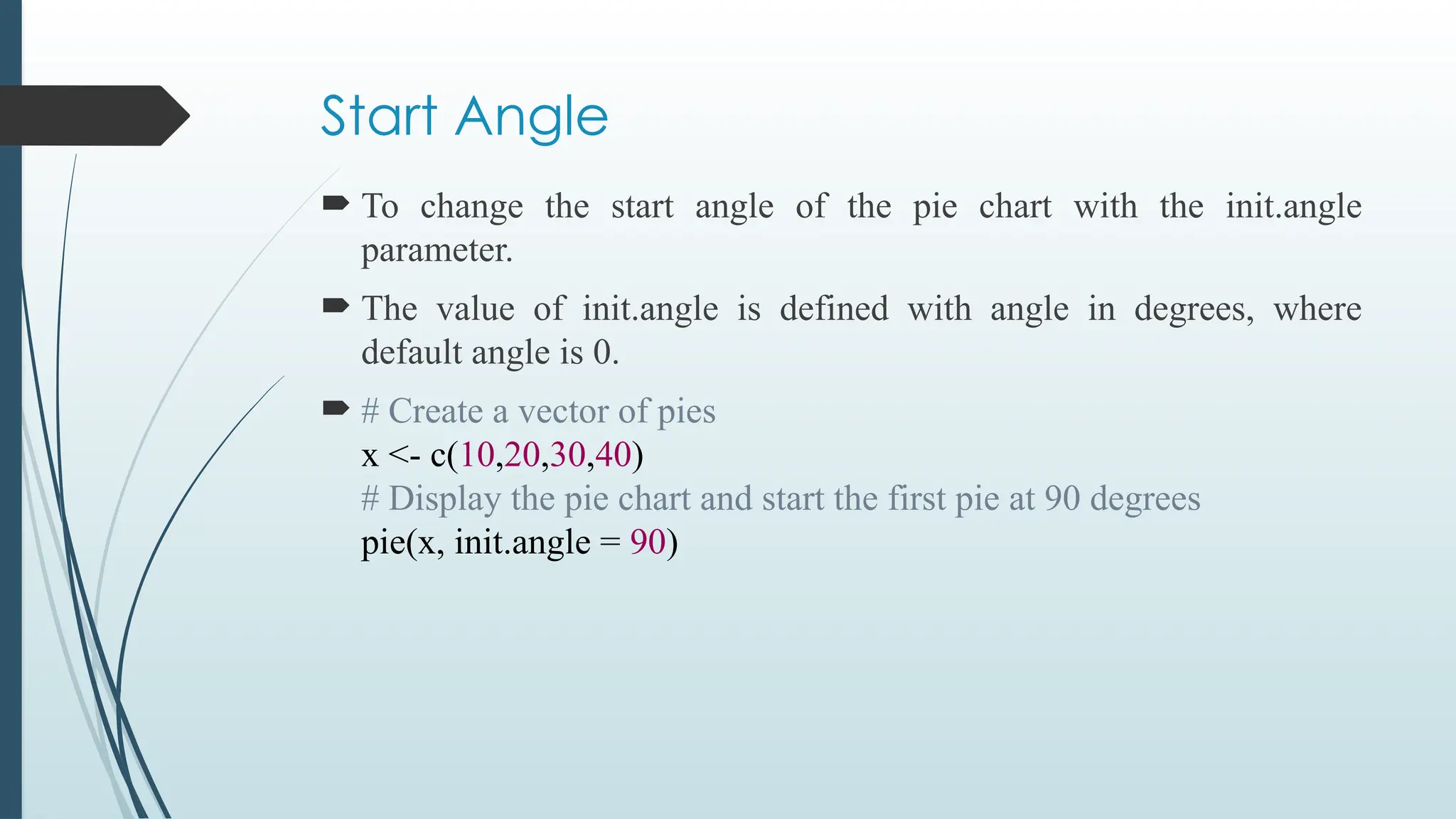
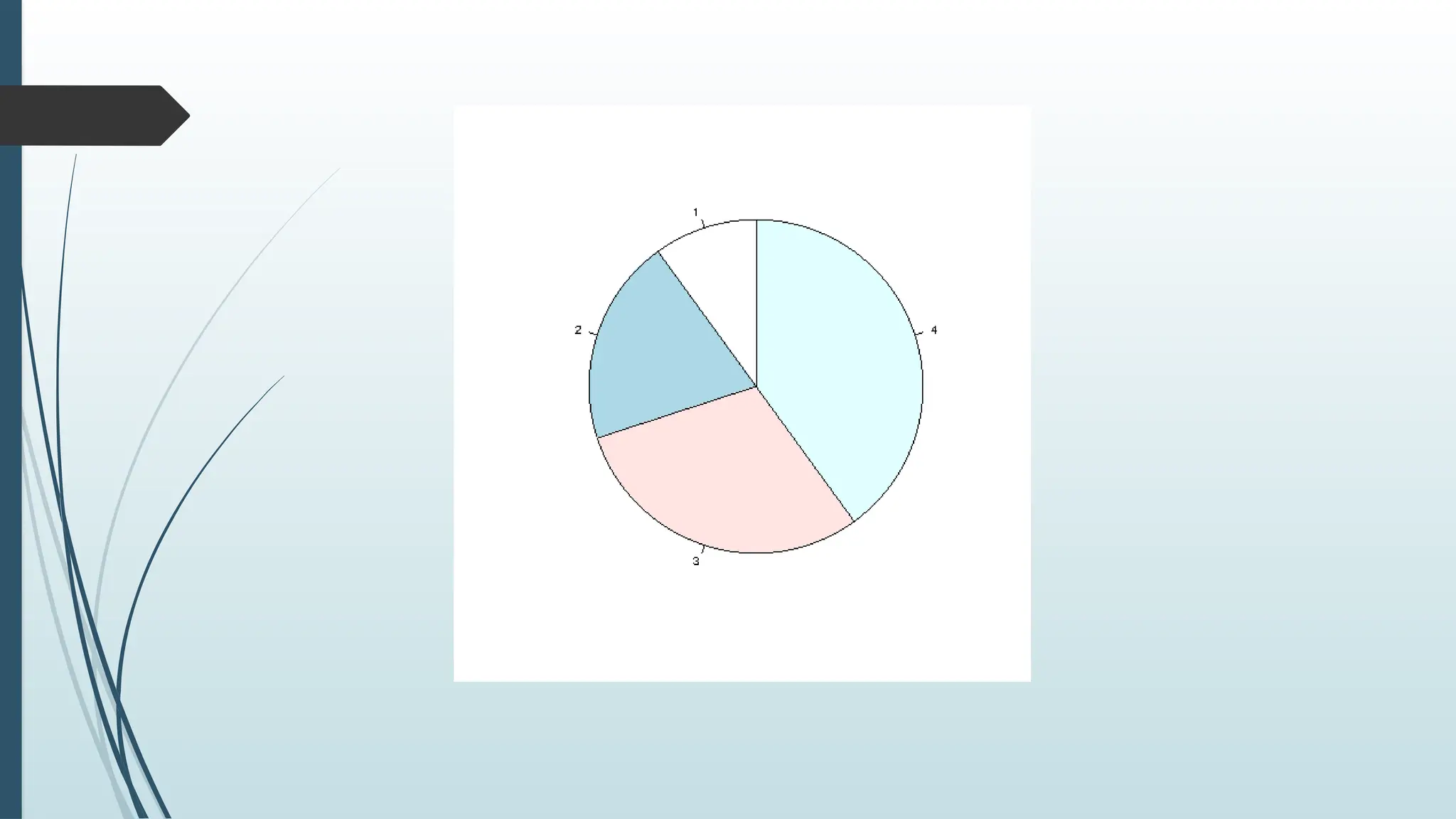
Start Angle
Tochange the start angle of the pie chart with the init.angle
parameter.
The value of init.angle is defined with angle in degrees, where
default angle is 0.
# Create a vector of pies
x <- c(10,20,30,40)
# Display the pie chart and start the first pie at 90 degrees
pie(x, init.angle = 90)
136.
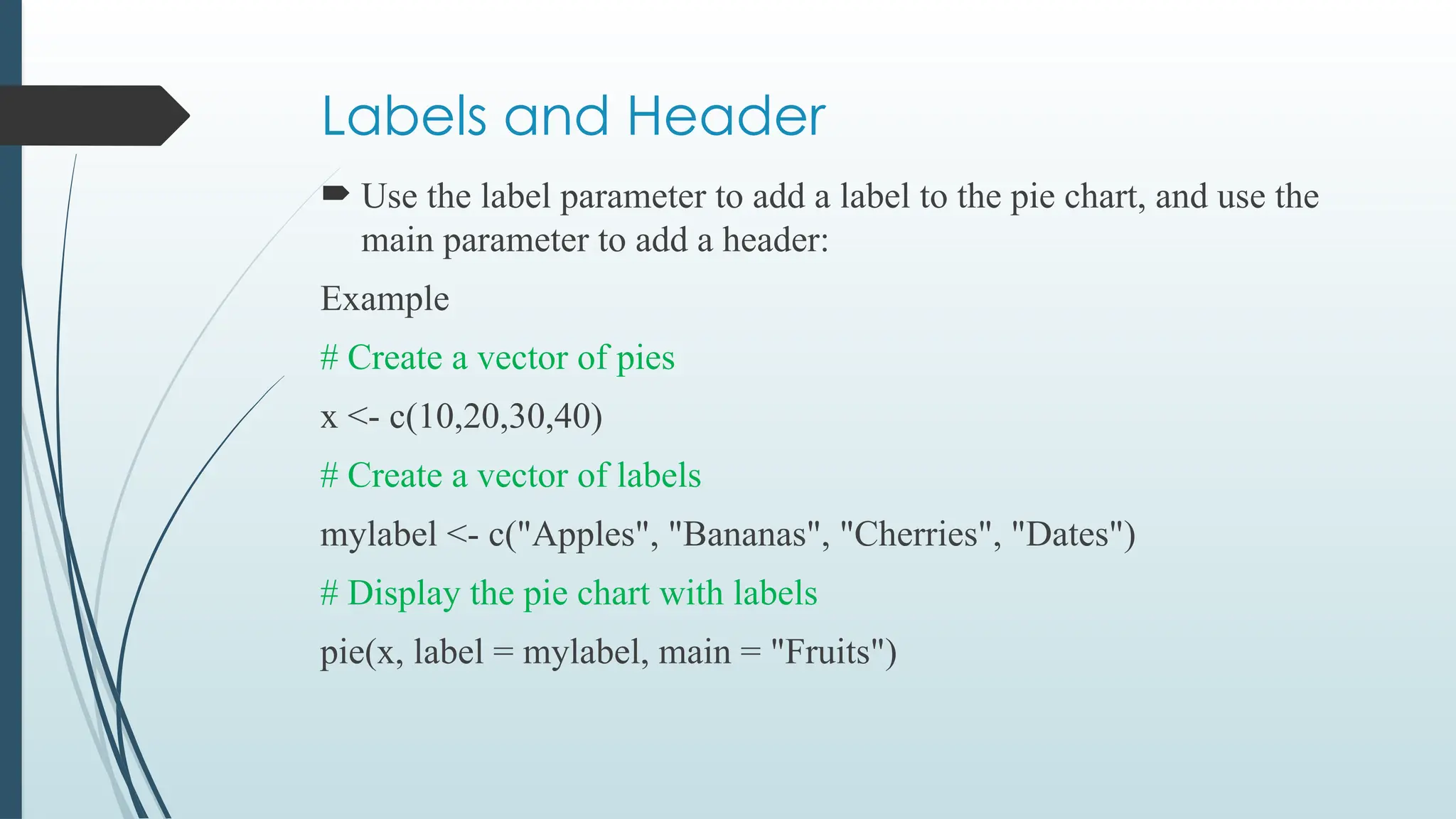
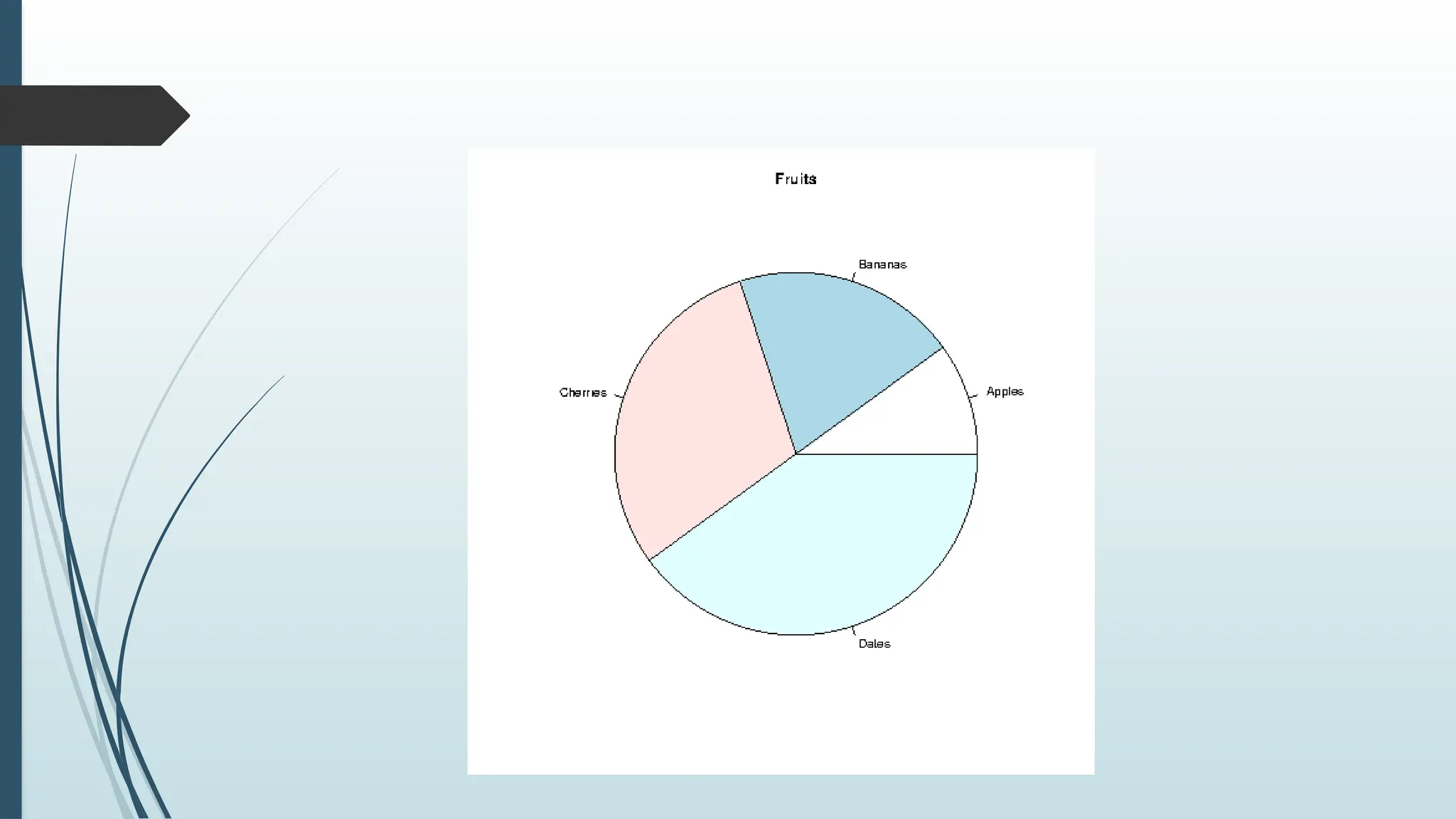
Labels and Header
Use the label parameter to add a label to the pie chart, and use the
main parameter to add a header:
Example
# Create a vector of pies
x <- c(10,20,30,40)
# Create a vector of labels
mylabel <- c("Apples", "Bananas", "Cherries", "Dates")
# Display the pie chart with labels
pie(x, label = mylabel, main = "Fruits")
138.
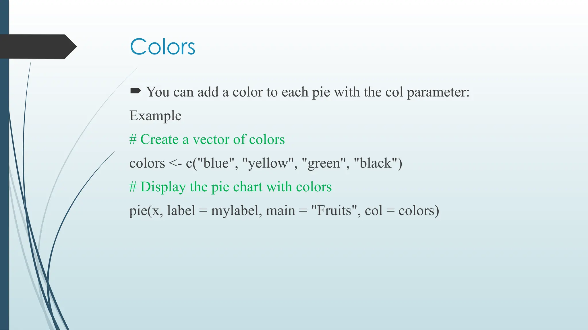
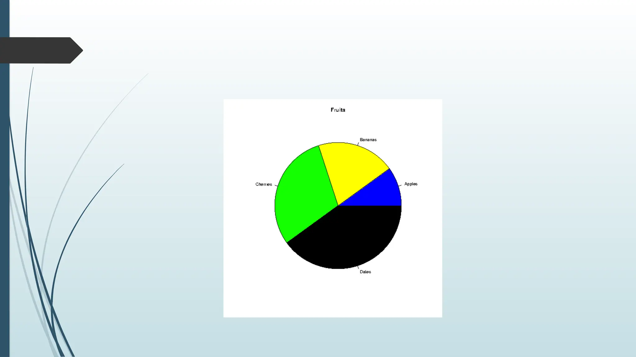
Colors
You canadd a color to each pie with the col parameter:
Example
# Create a vector of colors
colors <- c("blue", "yellow", "green", "black")
# Display the pie chart with colors
pie(x, label = mylabel, main = "Fruits", col = colors)
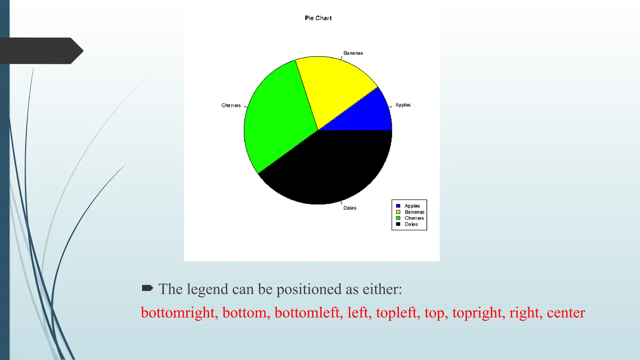
140.
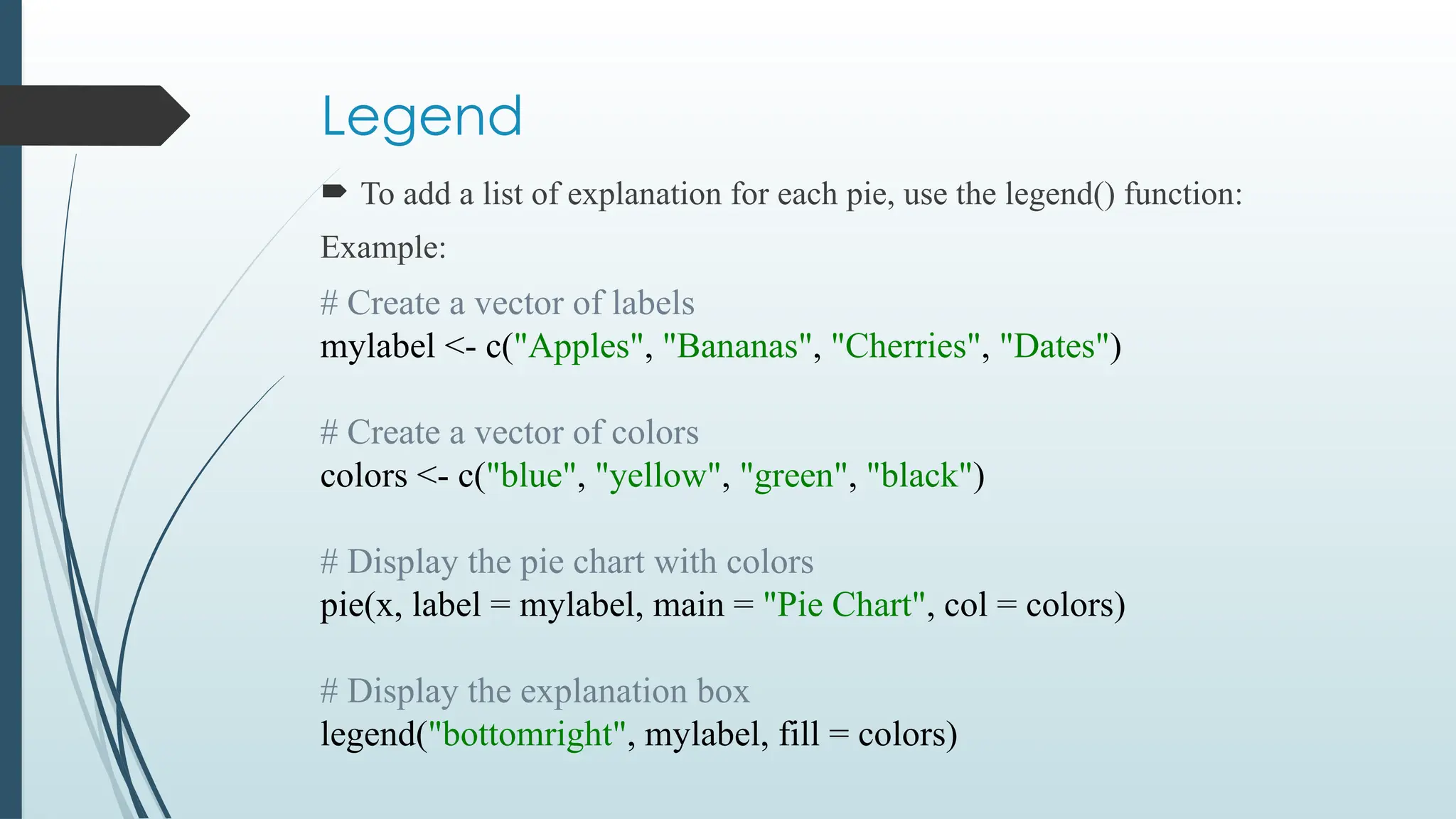
Legend
To adda list of explanation for each pie, use the legend() function:
Example:
# Create a vector of labels
mylabel <- c("Apples", "Bananas", "Cherries", "Dates")
# Create a vector of colors
colors <- c("blue", "yellow", "green", "black")
# Display the pie chart with colors
pie(x, label = mylabel, main = "Pie Chart", col = colors)
# Display the explanation box
legend("bottomright", mylabel, fill = colors)
141.
The legendcan be positioned as either:
bottomright, bottom, bottomleft, left, topleft, top, topright, right, center
142.
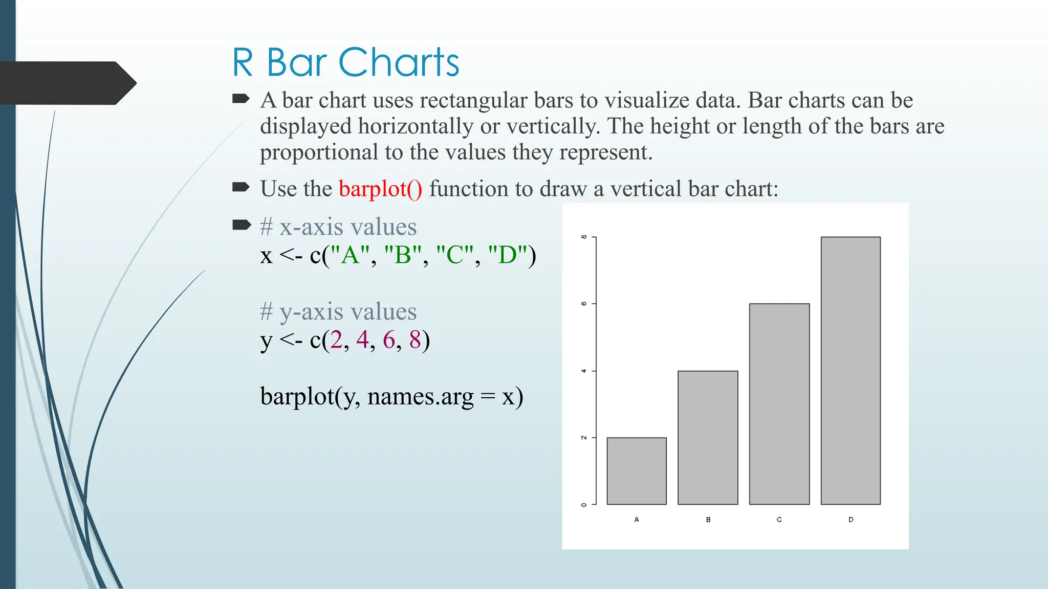
R Bar Charts
A bar chart uses rectangular bars to visualize data. Bar charts can be
displayed horizontally or vertically. The height or length of the bars are
proportional to the values they represent.
Use the barplot() function to draw a vertical bar chart:
# x-axis values
x <- c("A", "B", "C", "D")
# y-axis values
y <- c(2, 4, 6, 8)
barplot(y, names.arg = x)
143.
In the aboveexample:
The x variable represents values in the x-axis (A,B,C,D)
The y variable represents values in the y-axis (2,4,6,8)
Then we use the barplot() function to create a bar chart of the values
names.arg defines the names of each observation in the x-axis
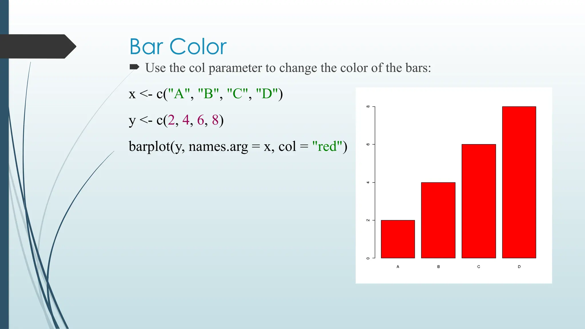
144.
Bar Color
Usethe col parameter to change the color of the bars:
x <- c("A", "B", "C", "D")
y <- c(2, 4, 6, 8)
barplot(y, names.arg = x, col = "red")
145.
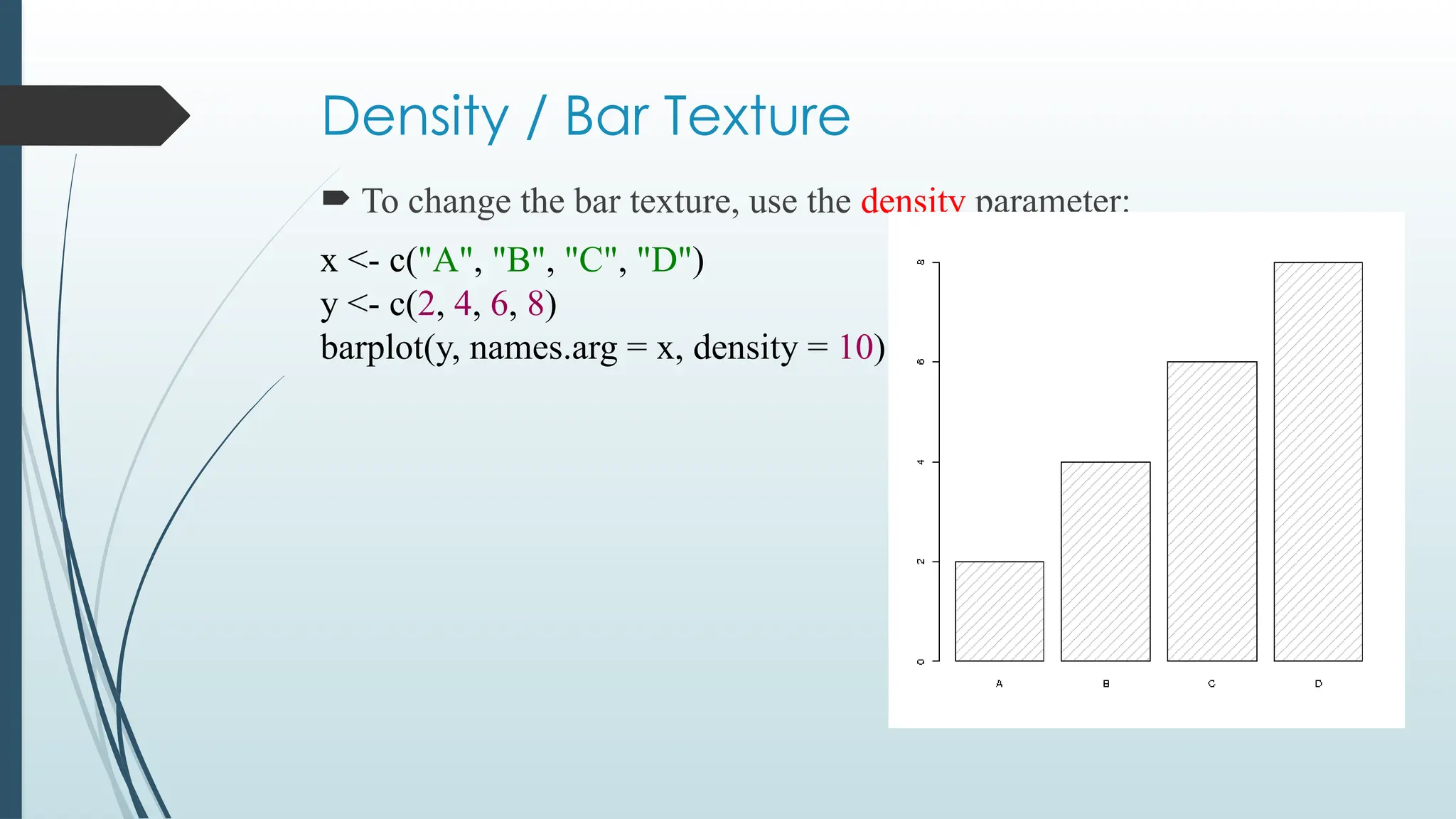
Density / BarTexture
To change the bar texture, use the density parameter:
x <- c("A", "B", "C", "D")
y <- c(2, 4, 6, 8)
barplot(y, names.arg = x, density = 10)
146.
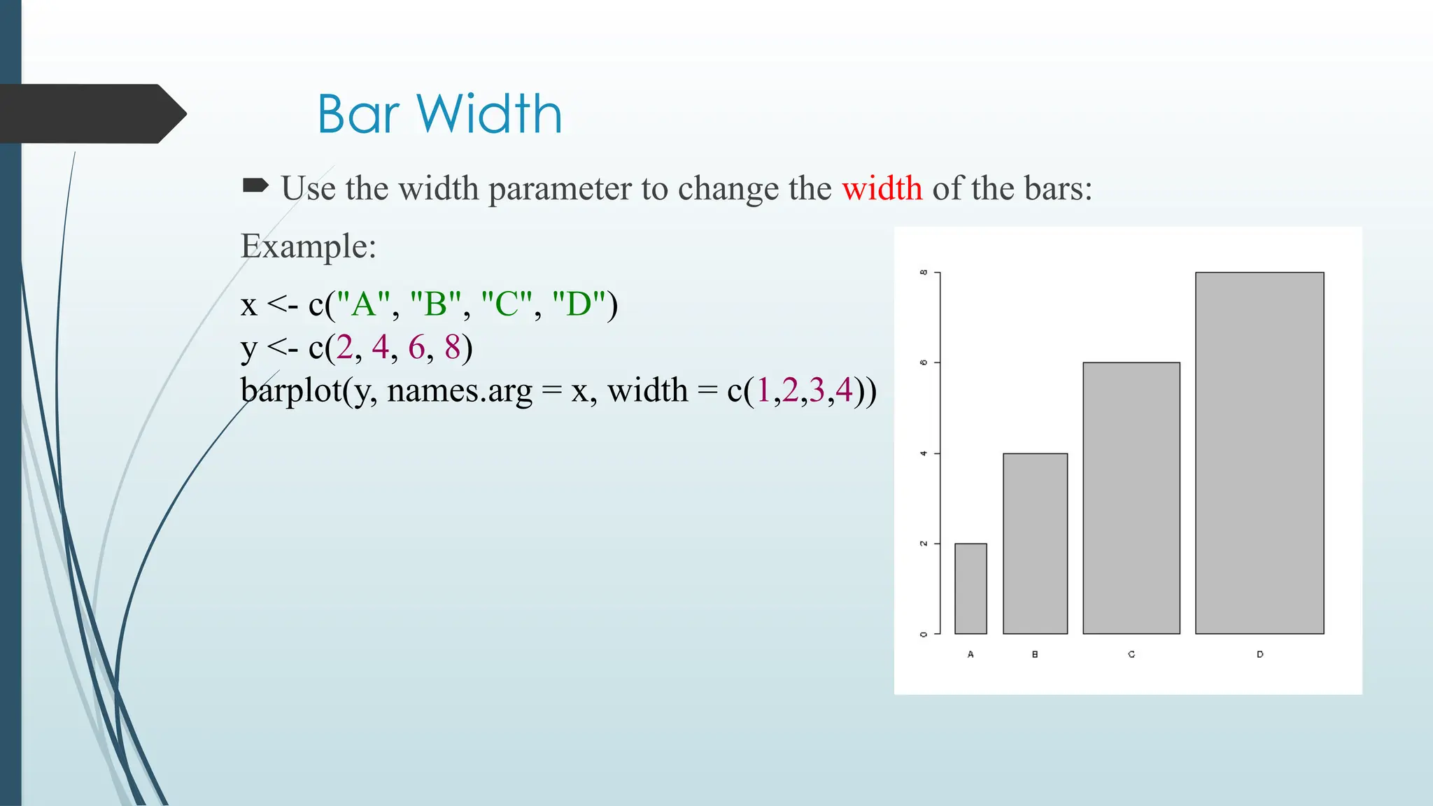
Bar Width
Usethe width parameter to change the width of the bars:
Example:
x <- c("A", "B", "C", "D")
y <- c(2, 4, 6, 8)
barplot(y, names.arg = x, width = c(1,2,3,4))
147.
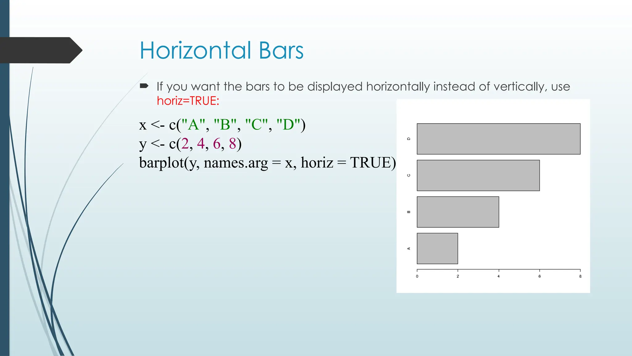
Horizontal Bars
Ifyou want the bars to be displayed horizontally instead of vertically, use
horiz=TRUE:
x <- c("A", "B", "C", "D")
y <- c(2, 4, 6, 8)
barplot(y, names.arg = x, horiz = TRUE)
Statistics Introduction
Statisticsis the science of analysing, reviewing and concluding data.
Some basic statistical numbers include:
• Mean, median and mode
• Minimum and maximum value
• Percentiles
• Variance and Standard Deviation
• Covariance and Correlation
• Probability distributions
The R language was developed by two statisticians. It has many
built-in functionalities, in addition to libraries for the exact purpose
of statistical analysis.
150.
R Data Set
A data set is a collection of data, often presented in a table.
There is a popular built-in data set in R called "mtcars" (Motor
Trend Car Road Tests), which is retrieved from the 1974 Motor
Trend US Magazine.
Example:
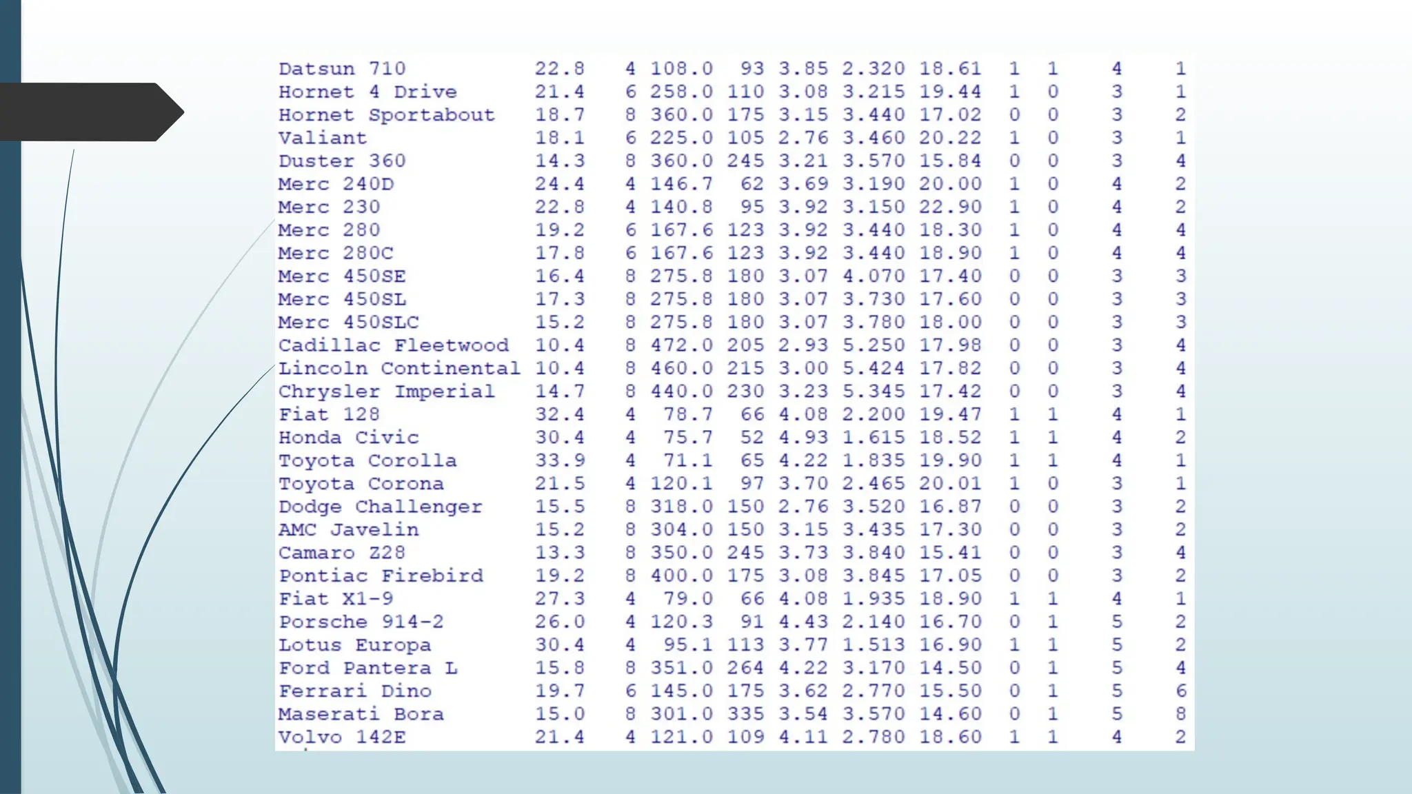
# Print the mtcars data set
mtcars
OUTPUT: next slide
152.
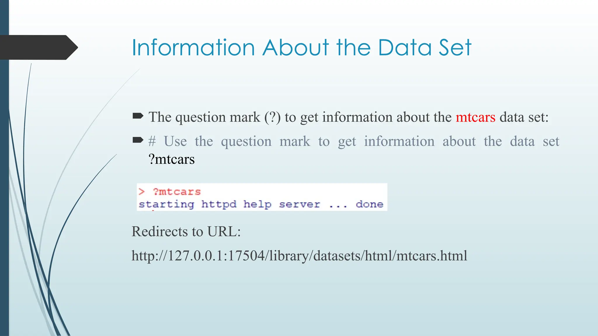
Information About theData Set
The question mark (?) to get information about the mtcars data set:
# Use the question mark to get information about the data set
?mtcars
Redirects to URL:
http://127.0.0.1:17504/library/datasets/html/mtcars.html
153.
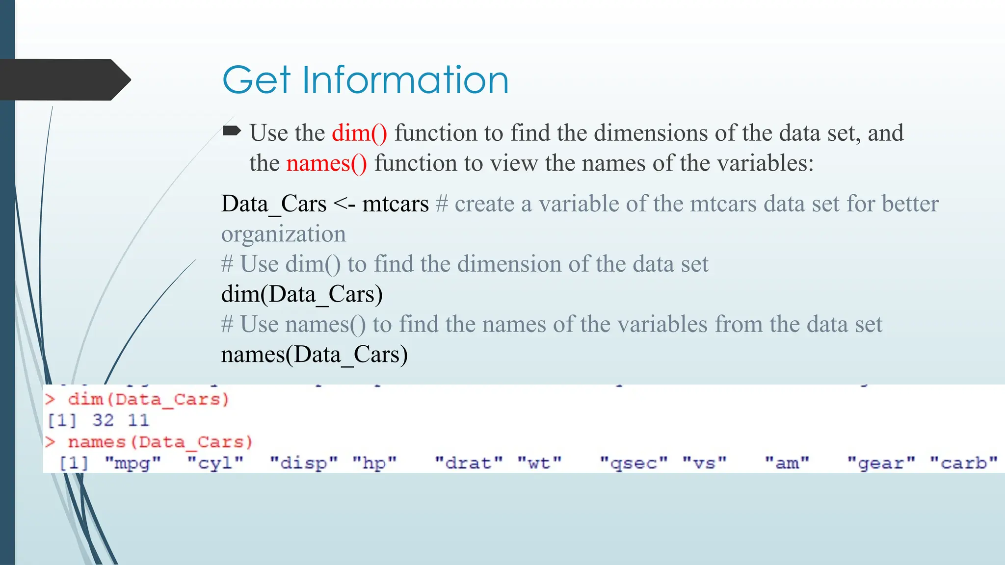
Get Information
Usethe dim() function to find the dimensions of the data set, and
the names() function to view the names of the variables:
Data_Cars <- mtcars # create a variable of the mtcars data set for better
organization
# Use dim() to find the dimension of the data set
dim(Data_Cars)
# Use names() to find the names of the variables from the data set
names(Data_Cars)
154.
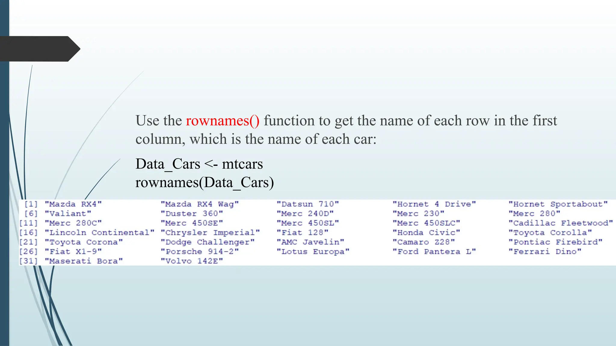
Use the rownames()function to get the name of each row in the first
column, which is the name of each car:
Data_Cars <- mtcars
rownames(Data_Cars)
155.
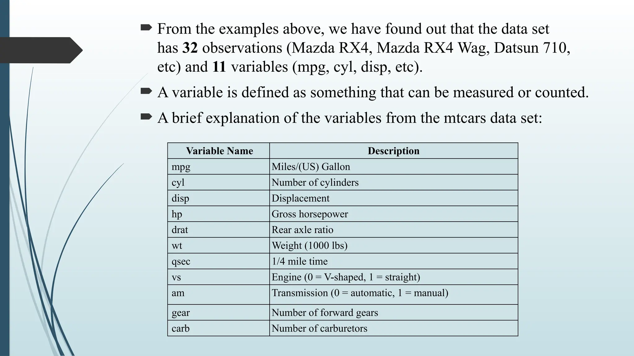
From theexamples above, we have found out that the data set
has 32 observations (Mazda RX4, Mazda RX4 Wag, Datsun 710,
etc) and 11 variables (mpg, cyl, disp, etc).
A variable is defined as something that can be measured or counted.
A brief explanation of the variables from the mtcars data set:
Variable Name Description
mpg Miles/(US) Gallon
cyl Number of cylinders
disp Displacement
hp Gross horsepower
drat Rear axle ratio
wt Weight (1000 lbs)
qsec 1/4 mile time
vs Engine (0 = V-shaped, 1 = straight)
am Transmission (0 = automatic, 1 = manual)
gear Number of forward gears
carb Number of carburetors
156.
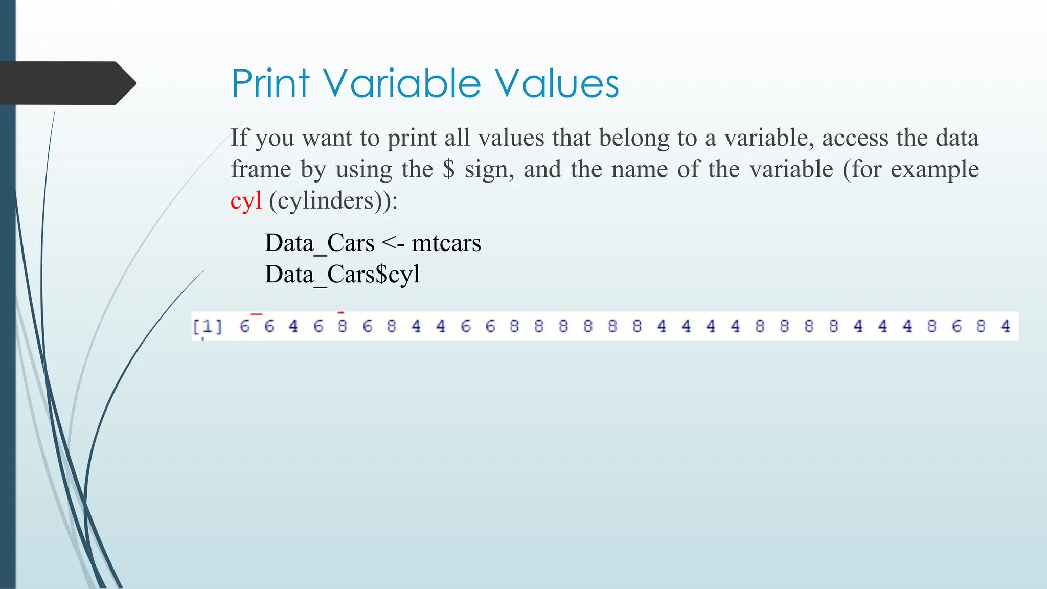
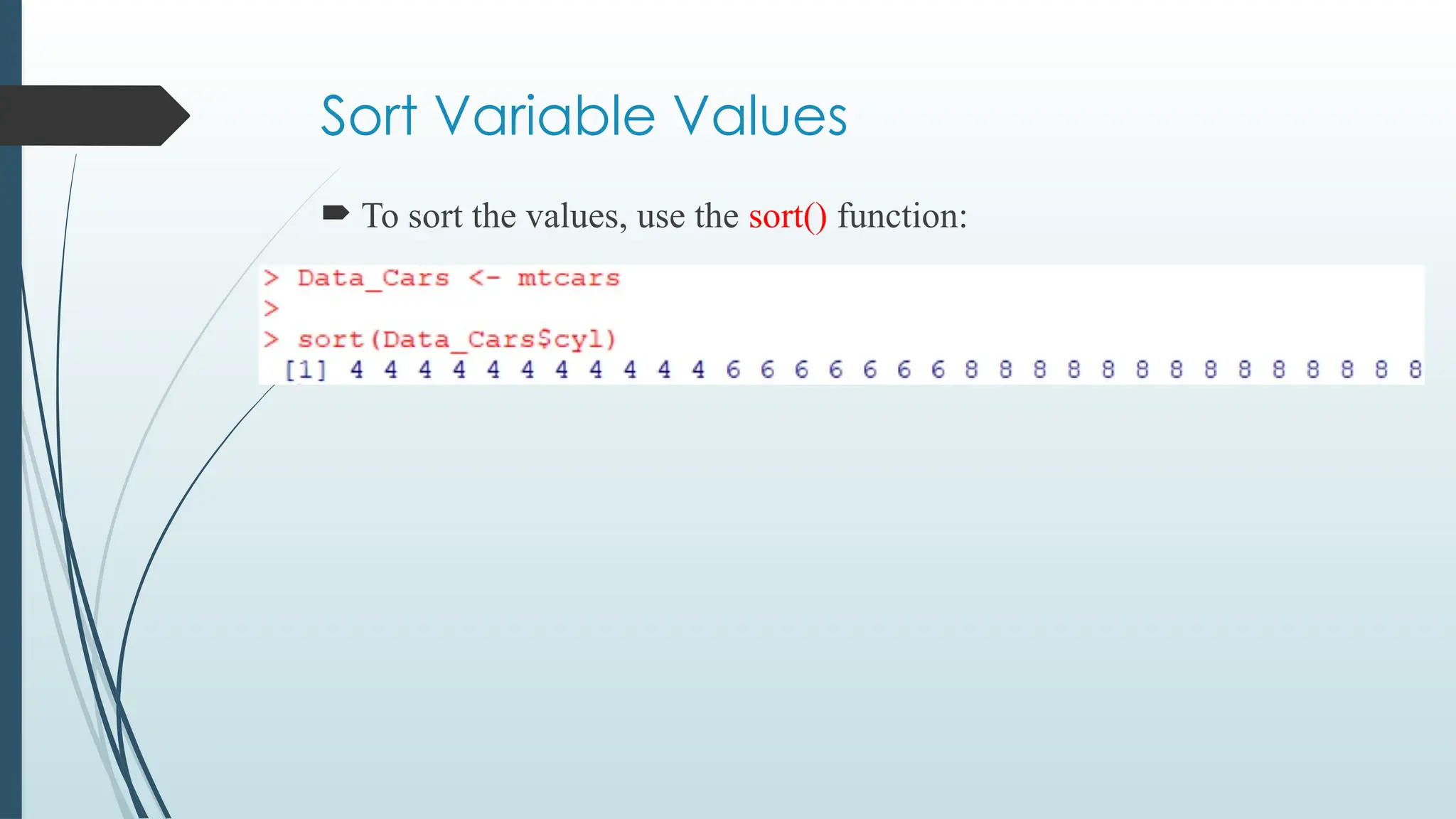
Print Variable Values
Ifyou want to print all values that belong to a variable, access the data
frame by using the $ sign, and the name of the variable (for example
cyl (cylinders)):
Data_Cars <- mtcars
Data_Cars$cyl
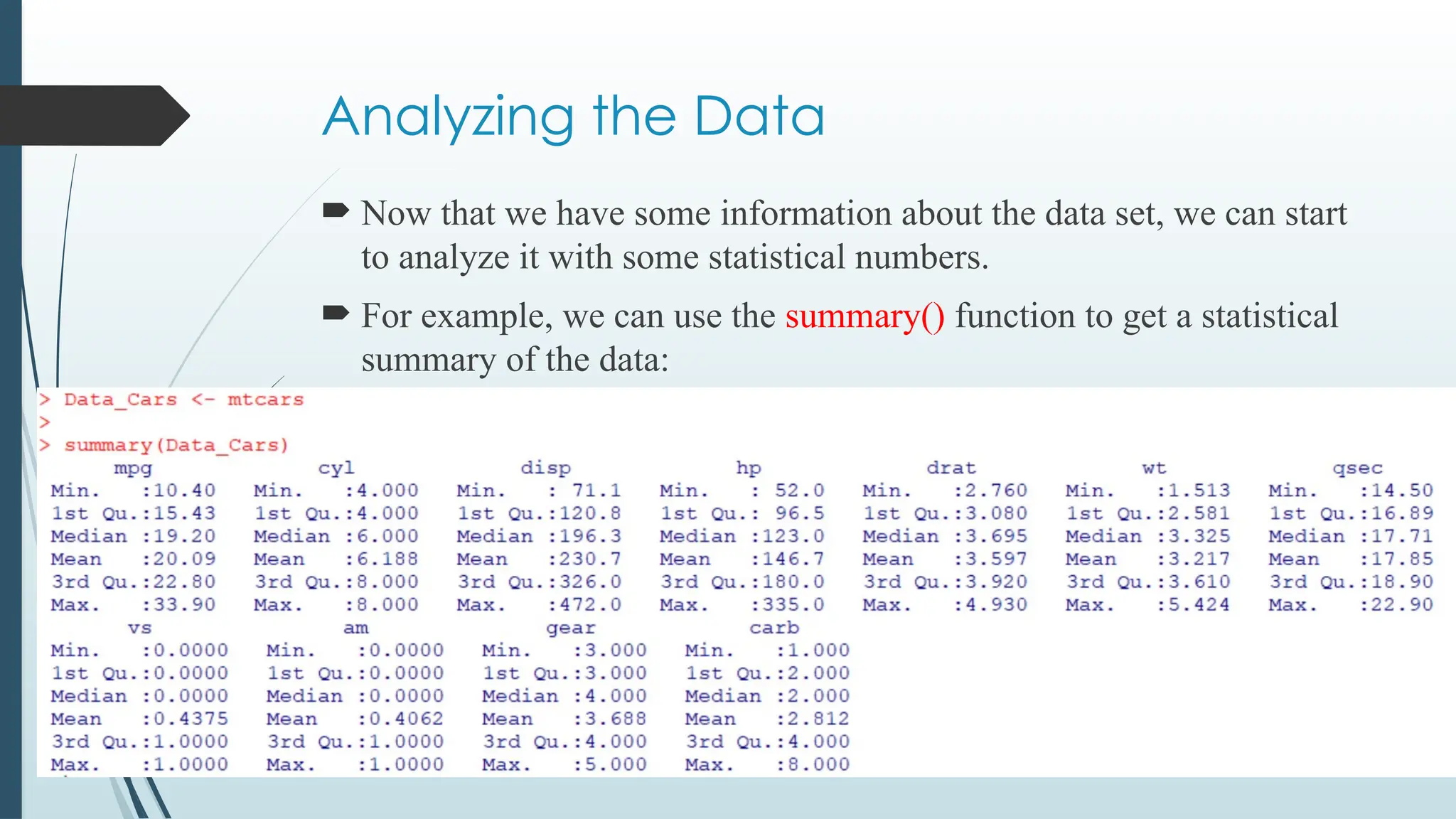
Analyzing the Data
Now that we have some information about the data set, we can start
to analyze it with some statistical numbers.
For example, we can use the summary() function to get a statistical
summary of the data:
159.
The summary()function returns six statistical numbers for each
variable:
• Min
• First quantile (percentile)
• Median
• Mean
• Third quantile (percentile)
• Max
160.
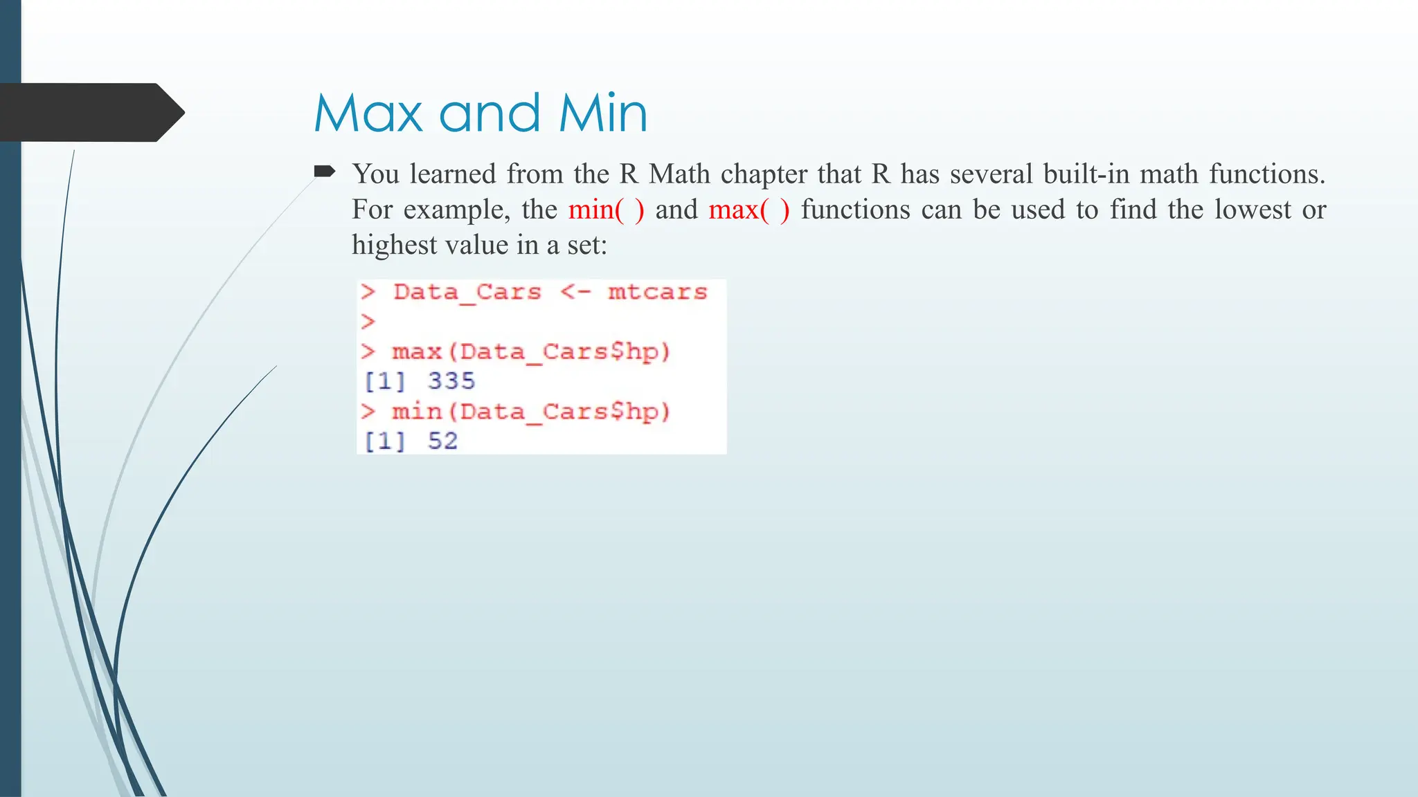
Max and Min
You learned from the R Math chapter that R has several built-in math functions.
For example, the min( ) and max( ) functions can be used to find the lowest or
highest value in a set:
161.
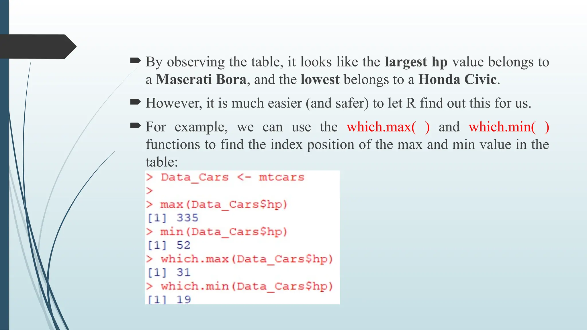
By observingthe table, it looks like the largest hp value belongs to
a Maserati Bora, and the lowest belongs to a Honda Civic.
However, it is much easier (and safer) to let R find out this for us.
For example, we can use the which.max( ) and which.min( )
functions to find the index position of the max and min value in the
table:
162.
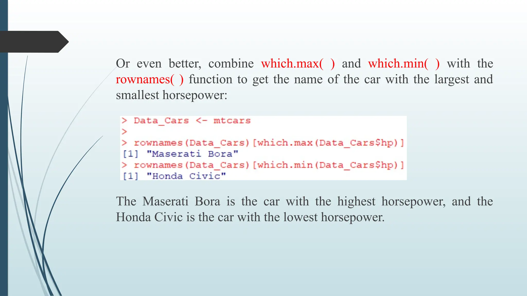
Or even better,combine which.max( ) and which.min( ) with the
rownames( ) function to get the name of the car with the largest and
smallest horsepower:
The Maserati Bora is the car with the highest horsepower, and the
Honda Civic is the car with the lowest horsepower.
163.
Outliers
Max andmin can also be used to detect outliers. An outlier is a data
point that differs from rest of the observations.
Example of data points that could have been outliers in the mtcars
data set:
• If maximum of forward gears of a car was 11
• If minimum of horsepower of a car was 0
• If maximum weight of a car was 50 000 lbs
164.
R Mean
In statistics,there are often three values that interest us:
• Mean - The average value
• Median - The middle value
• Mode - The most common value
165.
Mean
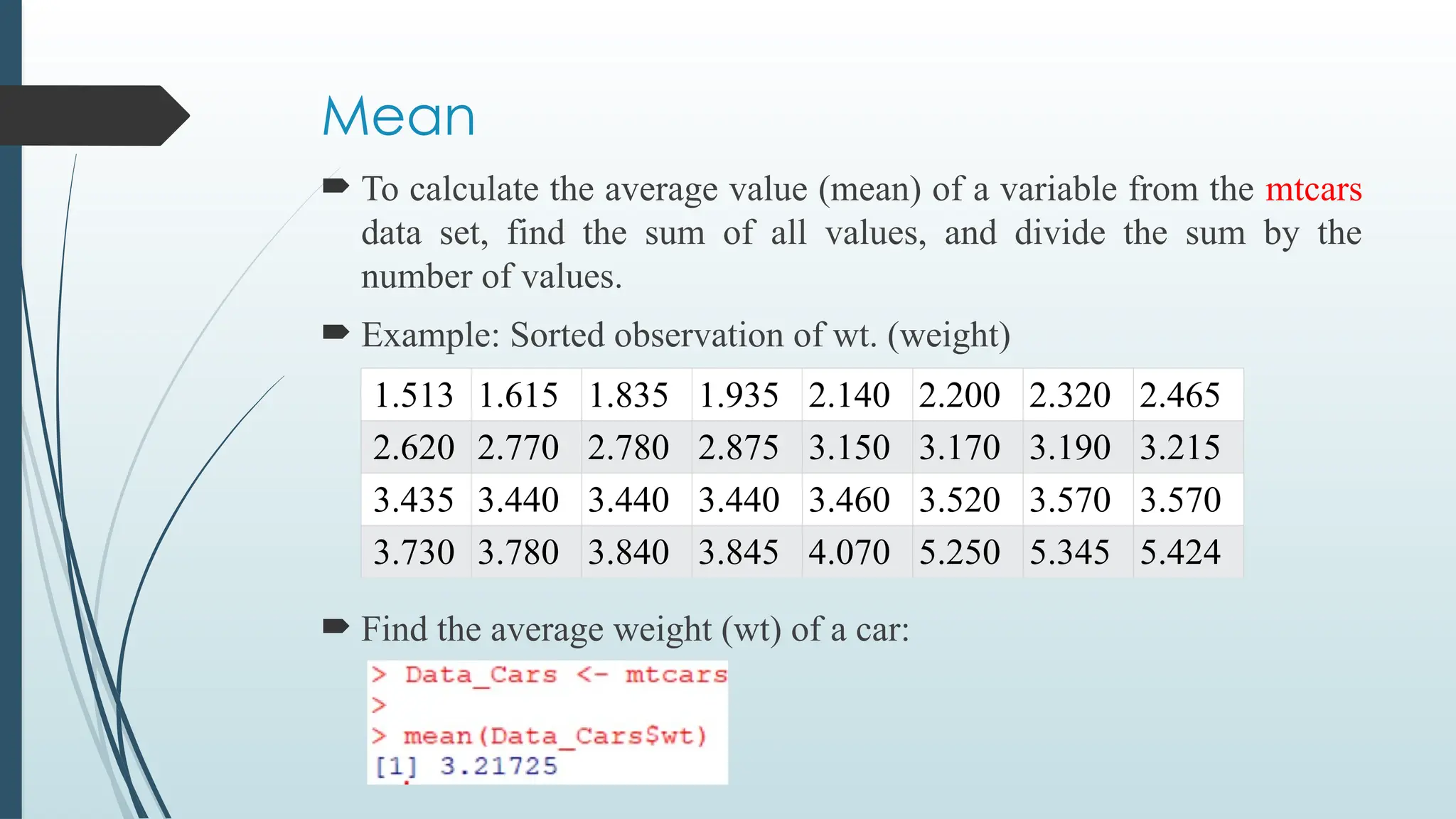
To calculatethe average value (mean) of a variable from the mtcars
data set, find the sum of all values, and divide the sum by the
number of values.
Example: Sorted observation of wt. (weight)
Find the average weight (wt) of a car:
1.513 1.615 1.835 1.935 2.140 2.200 2.320 2.465
2.620 2.770 2.780 2.875 3.150 3.170 3.190 3.215
3.435 3.440 3.440 3.440 3.460 3.520 3.570 3.570
3.730 3.780 3.840 3.845 4.070 5.250 5.345 5.424
166.
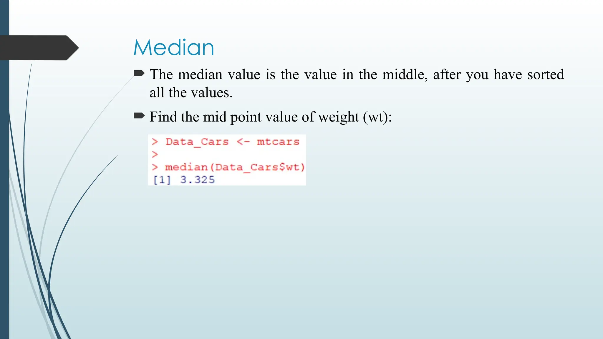
Median
The medianvalue is the value in the middle, after you have sorted
all the values.
Find the mid point value of weight (wt):
167.
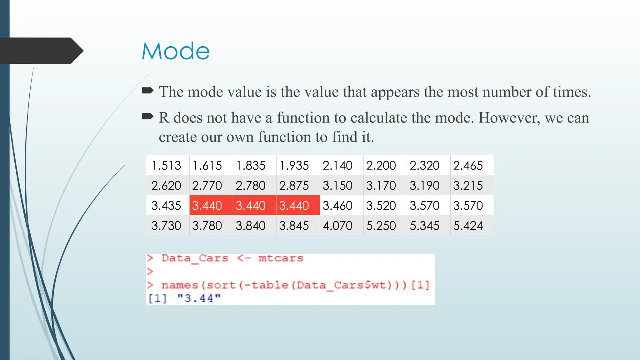
Mode
The modevalue is the value that appears the most number of times.
R does not have a function to calculate the mode. However, we can
create our own function to find it.
1.513 1.615 1.835 1.935 2.140 2.200 2.320 2.465
2.620 2.770 2.780 2.875 3.150 3.170 3.190 3.215
3.435 3.440 3.440 3.440 3.460 3.520 3.570 3.570
3.730 3.780 3.840 3.845 4.070 5.250 5.345 5.424
168.
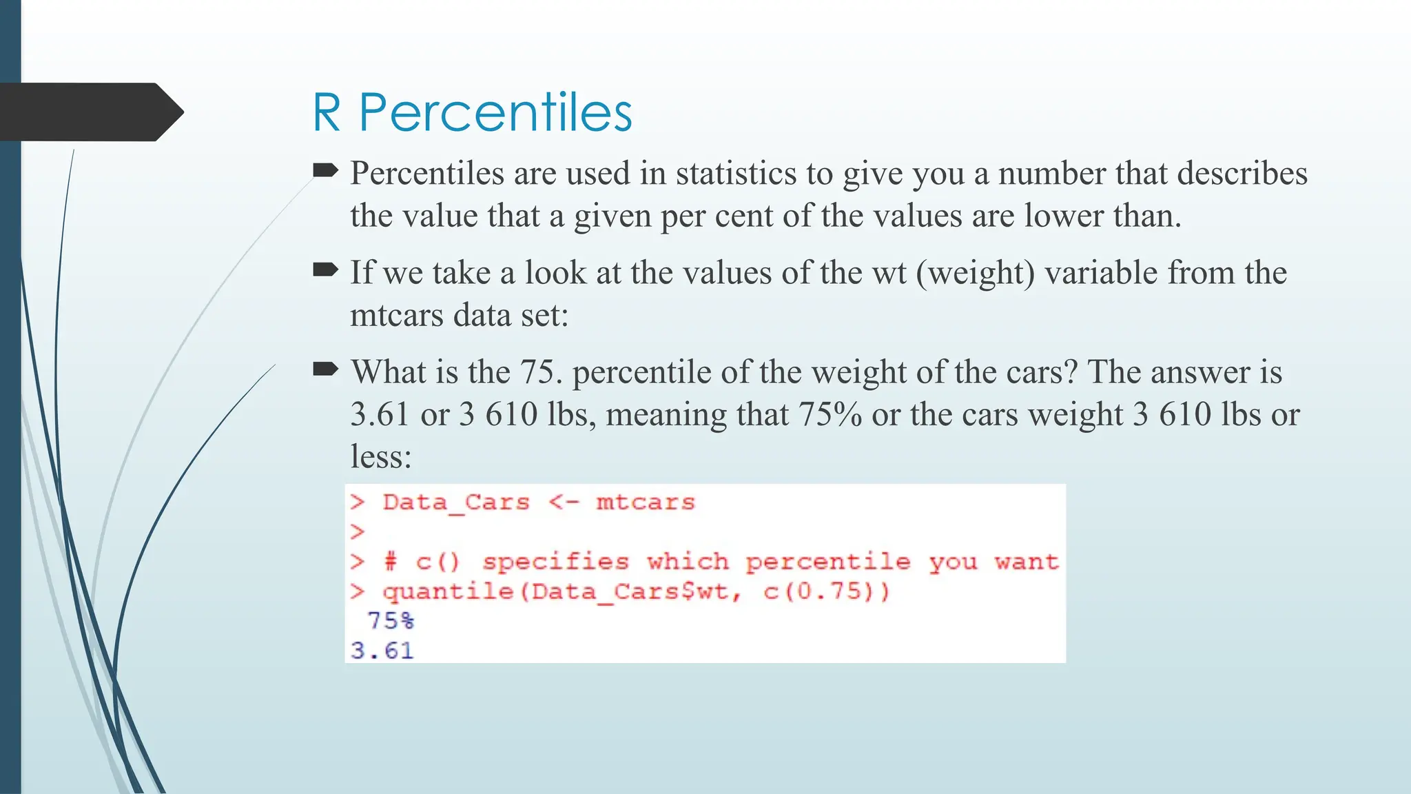
R Percentiles
Percentilesare used in statistics to give you a number that describes
the value that a given per cent of the values are lower than.
If we take a look at the values of the wt (weight) variable from the
mtcars data set:
What is the 75. percentile of the weight of the cars? The answer is
3.61 or 3 610 lbs, meaning that 75% or the cars weight 3 610 lbs or
less:
169.
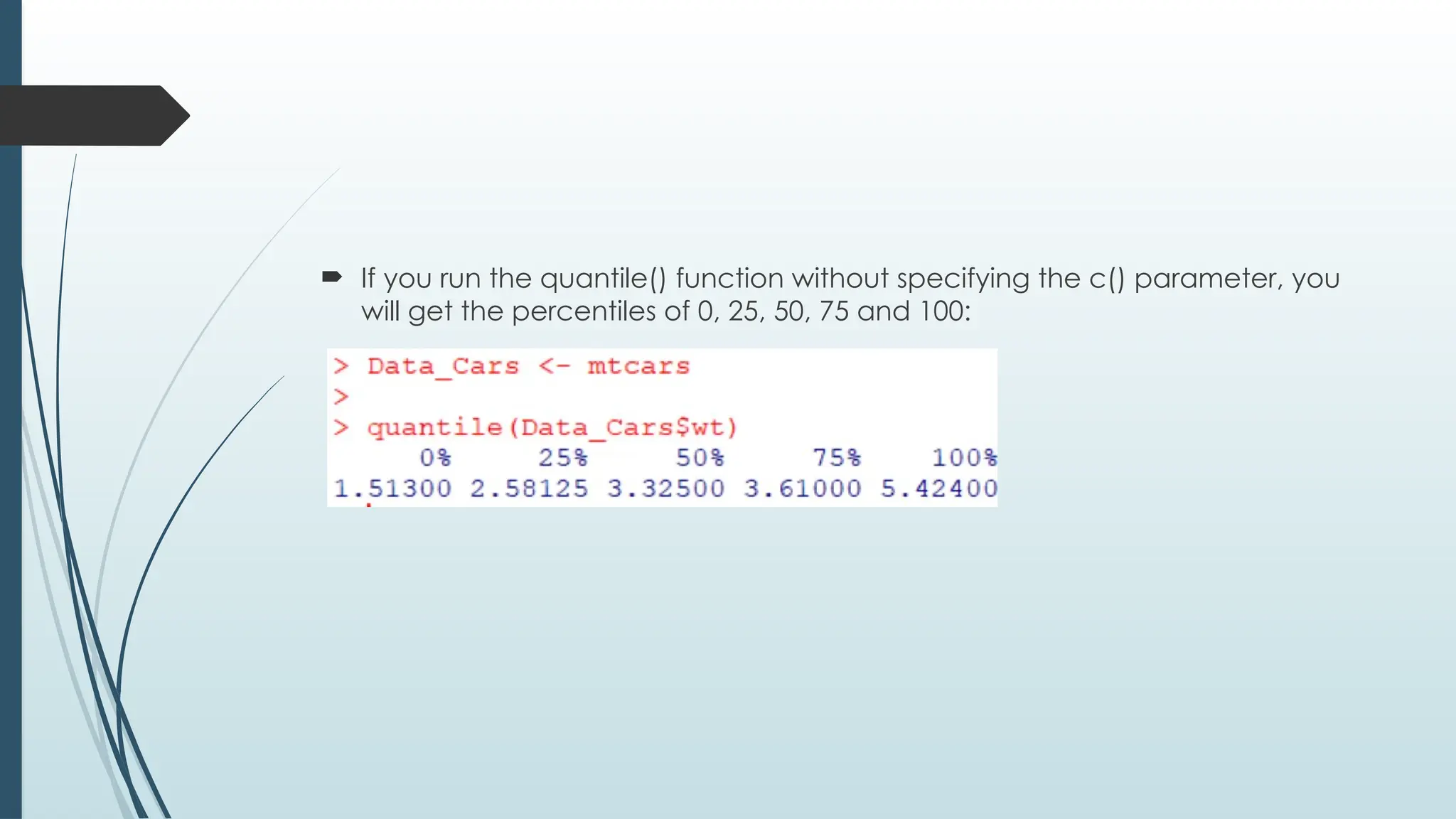
If yourun the quantile() function without specifying the c() parameter, you
will get the percentiles of 0, 25, 50, 75 and 100:
170.
Quartiles aredata divided into four parts, when sorted in an
ascending order:
• The value of the first quartile cuts off the first 25% of the data
• The value of the second quartile cuts off the first 50% of the data
• The value of the third quartile cuts off the first 75% of the data
• The value of the fourth quartile cuts off the 100% of the data
Editor's Notes
#83 A data frame in R is a two-dimensional, tabular data structure used to store data in the form of rows and columns, where each column can contain data of different types (such as numeric, character, or logical data). It is one of the most commonly used data structures in R for data analysis because it can hold a variety of data types and is easy to manipulate.
Here are some key features of data frames in R:
1. Structure:
Rows: Represent observations or instances in the dataset.
Columns: Represent variables or features associated with the observations.

![R Lists
A list in R can contain many different data types inside it. A list is a
collection of data which is ordered and changeable.
# List of strings
thislist <- list("apple", "banana", "cherry")
# Print the list
thislist
thislist[1]
thislist[1] <- "blackcurrant"
# Print the updated list
thislist](https://image.slidesharecdn.com/unitiv-250928165213-ca044c82/75/Unit-4-Statistical-Data-Analysis-for-BTech-5th-SEM-64-2048.jpg)
![Creating a string type matrix
thismatrix <- matrix(c("apple", "banana", "cherry", "orange"), nrow = 2, ncol = 2)
thismatrix
You can access the items by using [ ] brackets. The first number "1" in the bracket
specifies the row-position, while the second number "2" specifies the column-
position:](https://image.slidesharecdn.com/unitiv-250928165213-ca044c82/75/Unit-4-Statistical-Data-Analysis-for-BTech-5th-SEM-73-2048.jpg)
![The whole row can be accessed if you specify a comma after the
number in the bracket:
The whole column can be accessed if you specify a comma before the
number in the bracket:
More than one row can be accessed if you use the c() function:
thismatrix <- matrix(c("apple", "banana", "cherry", "orange", "grape",
"pineapple", "pear", "melon", "fig"), nrow = 3, ncol = 3)
thismatrix[c(1,2),]](https://image.slidesharecdn.com/unitiv-250928165213-ca044c82/75/Unit-4-Statistical-Data-Analysis-for-BTech-5th-SEM-74-2048.jpg)
![Accessing Arrays
You can access the array elements by referring to the index position.
You can use the [] brackets to access the desired elements from an
array:](https://image.slidesharecdn.com/unitiv-250928165213-ca044c82/75/Unit-4-Statistical-Data-Analysis-for-BTech-5th-SEM-77-2048.jpg)
![Access Items in Frames
We can use single brackets [ ], double brackets [[ ]] or $
to access columns from a data frame:](https://image.slidesharecdn.com/unitiv-250928165213-ca044c82/75/Unit-4-Statistical-Data-Analysis-for-BTech-5th-SEM-86-2048.jpg)
![Access Factors
To access the items in a factor, refer to the index number, using []
brackets:](https://image.slidesharecdn.com/unitiv-250928165213-ca044c82/75/Unit-4-Statistical-Data-Analysis-for-BTech-5th-SEM-101-2048.jpg)
![ However, if you have already specified it inside the levels argument,
it will work:
music_genre <-
factor(c("Jazz", "Rock", "Classic", "Classic", "Pop", "Jazz", "Rock", "J
azz"), levels = c("Classic", "Jazz", "Pop", "Rock", "Opera"))
music_genre[3] <- "Opera"
music_genre[3]](https://image.slidesharecdn.com/unitiv-250928165213-ca044c82/75/Unit-4-Statistical-Data-Analysis-for-BTech-5th-SEM-103-2048.jpg)


![R Lists
A list in R can contain many different data types inside it. A list is a
collection of data which is ordered and changeable.
# List of strings
thislist <- list("apple", "banana", "cherry")
# Print the list
thislist
thislist[1]
thislist[1] <- "blackcurrant"
# Print the updated list
thislist](https://crownmelresort.com/image.slidesharecdn.com/unitiv-250928165213-ca044c82/75/Unit-4-Statistical-Data-Analysis-for-BTech-5th-SEM-64-2048.jpg)


![Creating a string type matrix
thismatrix <- matrix(c("apple", "banana", "cherry", "orange"), nrow = 2, ncol = 2)
thismatrix
You can access the items by using [ ] brackets. The first number "1" in the bracket
specifies the row-position, while the second number "2" specifies the column-
position:](https://crownmelresort.com/image.slidesharecdn.com/unitiv-250928165213-ca044c82/75/Unit-4-Statistical-Data-Analysis-for-BTech-5th-SEM-73-2048.jpg)
![The whole row can be accessed if you specify a comma after the
number in the bracket:
The whole column can be accessed if you specify a comma before the
number in the bracket:
More than one row can be accessed if you use the c() function:
thismatrix <- matrix(c("apple", "banana", "cherry", "orange", "grape",
"pineapple", "pear", "melon", "fig"), nrow = 3, ncol = 3)
thismatrix[c(1,2),]](https://crownmelresort.com/image.slidesharecdn.com/unitiv-250928165213-ca044c82/75/Unit-4-Statistical-Data-Analysis-for-BTech-5th-SEM-74-2048.jpg)


![Accessing Arrays
You can access the array elements by referring to the index position.
You can use the [] brackets to access the desired elements from an
array:](https://crownmelresort.com/image.slidesharecdn.com/unitiv-250928165213-ca044c82/75/Unit-4-Statistical-Data-Analysis-for-BTech-5th-SEM-77-2048.jpg)


![Access Items in Frames
We can use single brackets [ ], double brackets [[ ]] or $
to access columns from a data frame:](https://crownmelresort.com/image.slidesharecdn.com/unitiv-250928165213-ca044c82/75/Unit-4-Statistical-Data-Analysis-for-BTech-5th-SEM-86-2048.jpg)


![Access Factors
To access the items in a factor, refer to the index number, using []
brackets:](https://crownmelresort.com/image.slidesharecdn.com/unitiv-250928165213-ca044c82/75/Unit-4-Statistical-Data-Analysis-for-BTech-5th-SEM-101-2048.jpg)

![ However, if you have already specified it inside the levels argument,
it will work:
music_genre <-
factor(c("Jazz", "Rock", "Classic", "Classic", "Pop", "Jazz", "Rock", "J
azz"), levels = c("Classic", "Jazz", "Pop", "Rock", "Opera"))
music_genre[3] <- "Opera"
music_genre[3]](https://crownmelresort.com/image.slidesharecdn.com/unitiv-250928165213-ca044c82/75/Unit-4-Statistical-Data-Analysis-for-BTech-5th-SEM-103-2048.jpg)


![Basics of R programming for analytics [Autosaved] (1).pdf](https://cdn.slidesharecdn.com/ss_thumbnails/basicsofrprogrammingforanalyticsautosaved1-240916080545-0682f8c8-thumbnail.jpg?width=640&height=640&fit=bounds)