Big_DM_24_MS_Topic_02_Understanding Data.pdf

1
“In God we trust.
All others must bring data.” by W. Edwards Deming
Data

2
Chapter 2. Data, Measurements, and Data
Preprocessing
❑ Data Types
❑ Statics of Data
❑ Similarity and Distance Measures
❑ Data Quality, Data Cleaning and Data Integration
❑ Data Transformation
❑ Dimensionality Reduction
❑ Summary

3
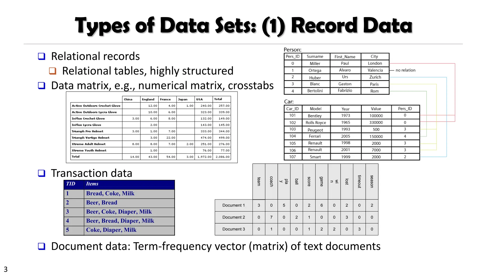
Types of Data Sets: (1) Record Data
❑ Relational records
❑ Relational tables, highly structured
❑ Data matrix, e.g., numerical matrix, crosstabs
❑ Transaction data
❑ Document data: Term-frequency vector (matrix) of text documents
Document 1
season
timeout
lost
wi
n
game
score
ball
pla
y
coach
team
Document 2
Document 3
3 0 5 0 2 6 0 2 0 2
0
0
7 0 2 1 0 0 3 0 0
1 0 0 1 2 2 0 3 0
TID Items
1 Bread, Coke, Milk
2 Beer, Bread
3 Beer, Coke, Diaper, Milk
4 Beer, Bread, Diaper, Milk
5 Coke, Diaper, Milk

4
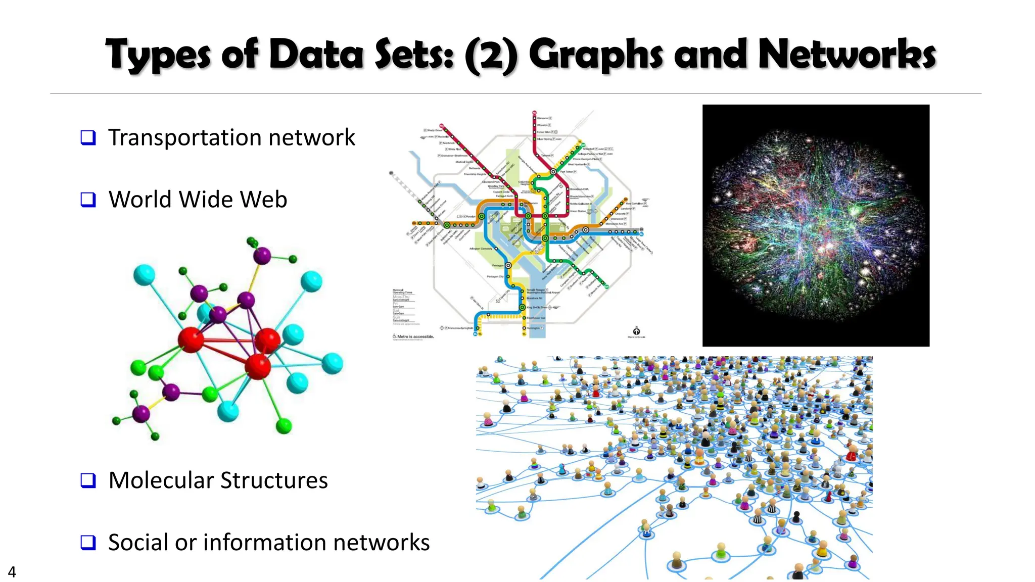
Types of Data Sets: (2) Graphs and Networks
❑ Transportation network
❑ World Wide Web
❑ Molecular Structures
❑ Social or information networks

5
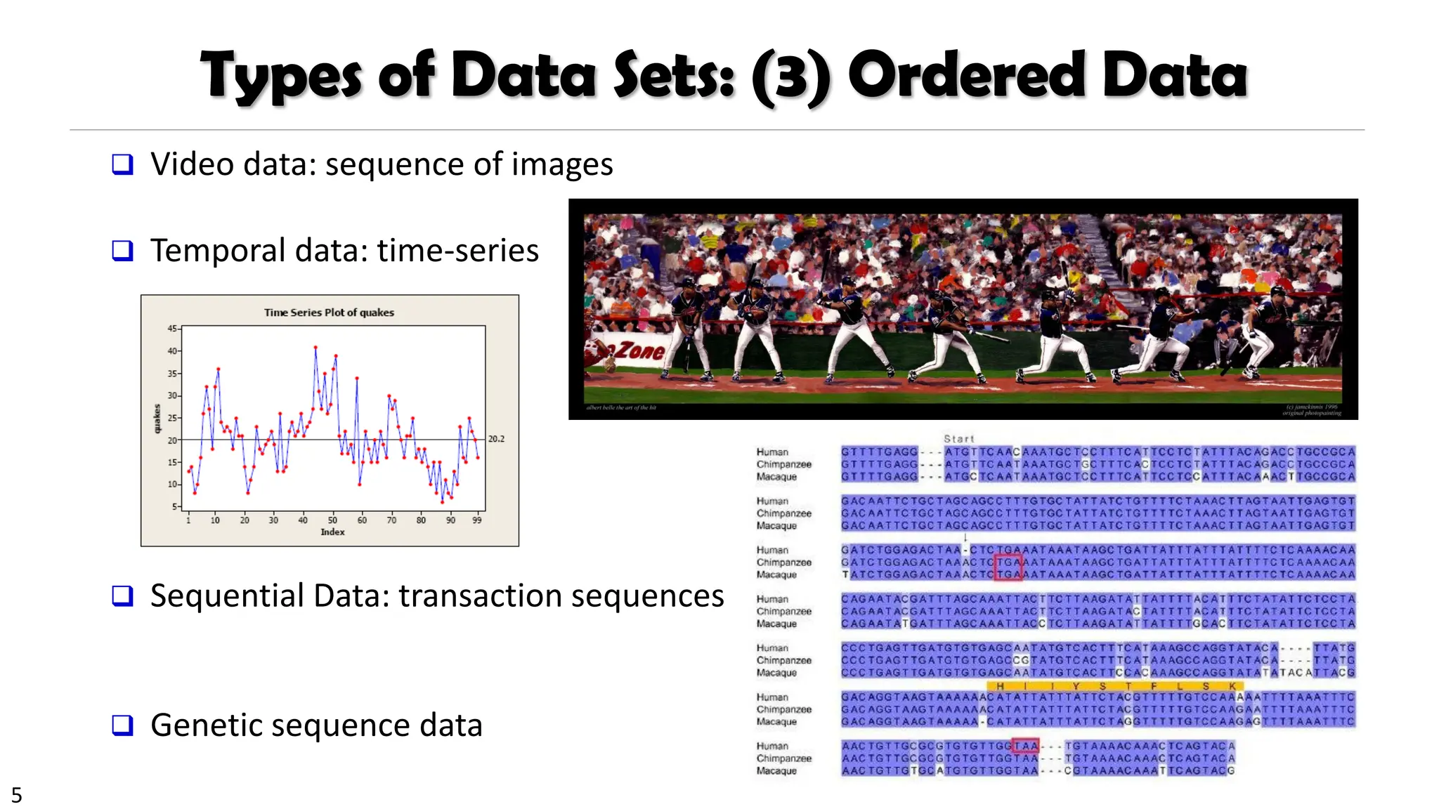
Types of Data Sets: (3) Ordered Data
❑ Video data: sequence of images
❑ Temporal data: time-series
❑ Sequential Data: transaction sequences
❑ Genetic sequence data

6
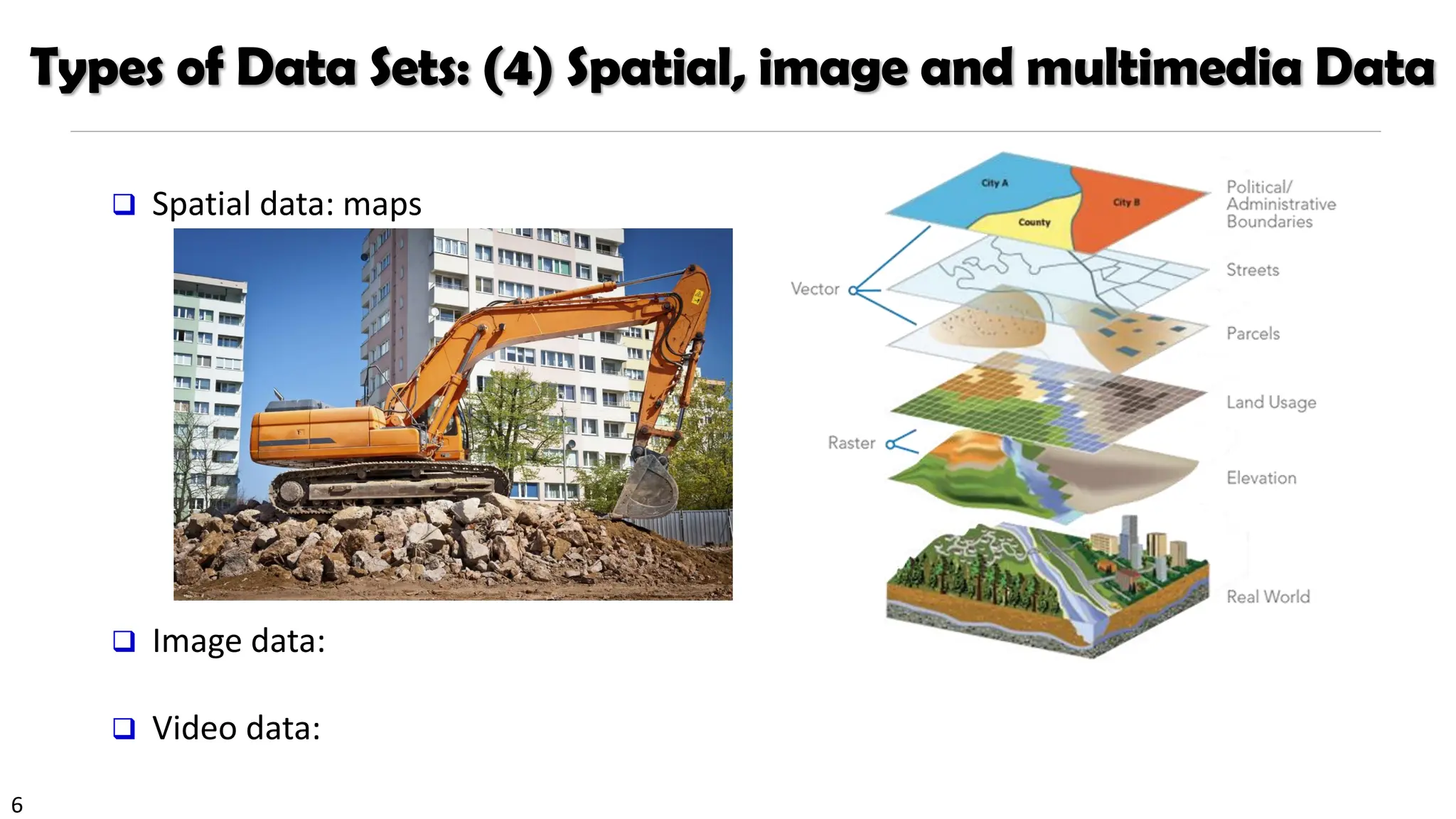
Types of Data Sets: (4) Spatial, image and multimedia Data
❑ Spatial data: maps
❑ Image data:
❑ Video data:

7
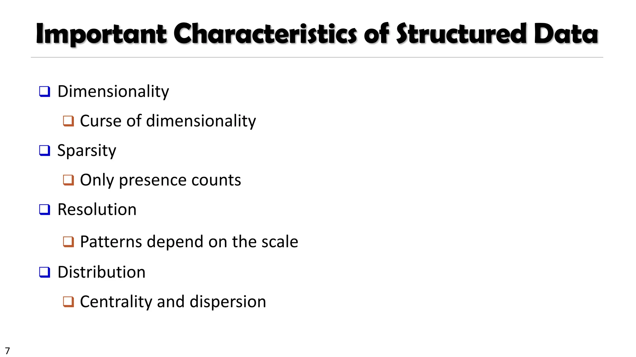
Important Characteristics of Structured Data
❑ Dimensionality
❑ Curse of dimensionality
❑ Sparsity
❑ Only presence counts
❑ Resolution
❑ Patterns depend on the scale
❑ Distribution
❑ Centrality and dispersion

8
Data Objects
❑ Data sets are made up of data objects
❑ A data object represents an entity
❑ Examples:
❑ sales database: customers, store items, sales
❑ medical database: patients, treatments
❑ university database: students, professors, courses
❑ Also called samples , examples, instances, data points, objects, tuples
❑ Data objects are described by attributes
❑ Database rows → data objects; columns → attributes

9
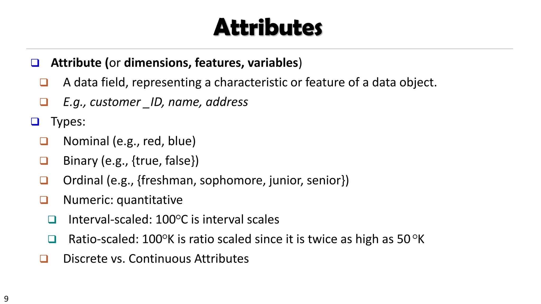
Attributes
❑ Attribute (or dimensions, features, variables)
❑ A data field, representing a characteristic or feature of a data object.
❑ E.g., customer _ID, name, address
❑ Types:
❑ Nominal (e.g., red, blue)
❑ Binary (e.g., {true, false})
❑ Ordinal (e.g., {freshman, sophomore, junior, senior})
❑ Numeric: quantitative
❑ Interval-scaled: 100○C is interval scales
❑ Ratio-scaled: 100○K is ratio scaled since it is twice as high as 50○K
❑ Discrete vs. Continuous Attributes

10
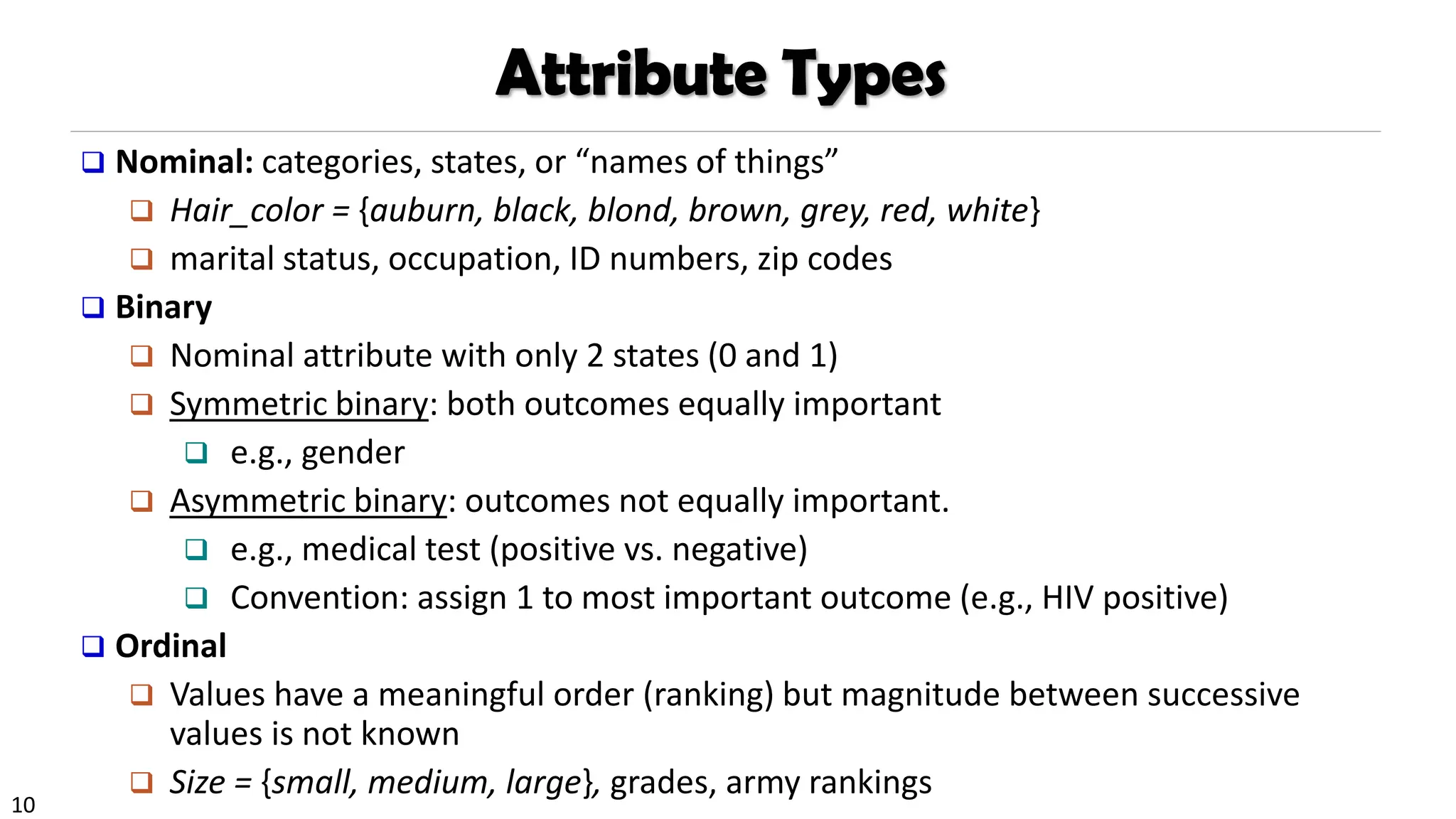
Attribute Types
❑ Nominal: categories, states, or “names of things”
❑ Hair_color = {auburn, black, blond, brown, grey, red, white}
❑ marital status, occupation, ID numbers, zip codes
❑ Binary
❑ Nominal attribute with only 2 states (0 and 1)
❑ Symmetric binary: both outcomes equally important
❑ e.g., gender
❑ Asymmetric binary: outcomes not equally important.
❑ e.g., medical test (positive vs. negative)
❑ Convention: assign 1 to most important outcome (e.g., HIV positive)
❑ Ordinal
❑ Values have a meaningful order (ranking) but magnitude between successive
values is not known
❑ Size = {small, medium, large}, grades, army rankings

11
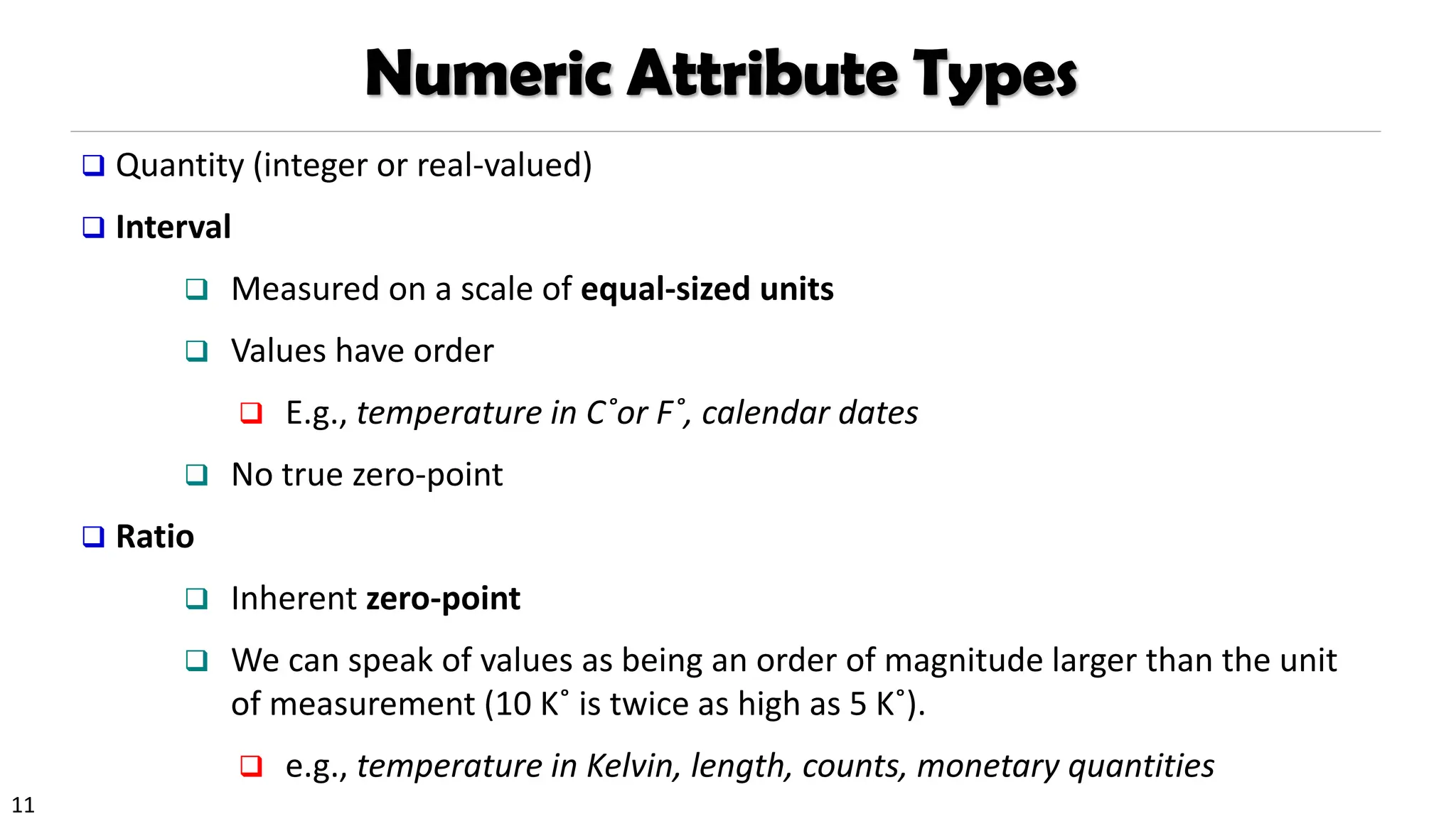
Numeric Attribute Types
❑ Quantity (integer or real-valued)
❑ Interval
❑ Measured on a scale of equal-sized units
❑ Values have order
❑ E.g., temperature in C˚or F˚, calendar dates
❑ No true zero-point
❑ Ratio
❑ Inherent zero-point
❑ We can speak of values as being an order of magnitude larger than the unit
of measurement (10 K˚ is twice as high as 5 K˚).
❑ e.g., temperature in Kelvin, length, counts, monetary quantities

12
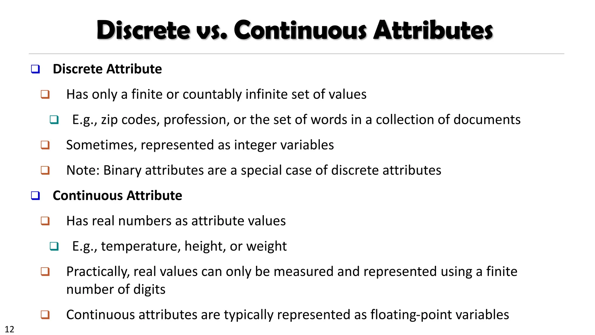
Discrete vs. Continuous Attributes
❑ Discrete Attribute
❑ Has only a finite or countably infinite set of values
❑ E.g., zip codes, profession, or the set of words in a collection of documents
❑ Sometimes, represented as integer variables
❑ Note: Binary attributes are a special case of discrete attributes
❑ Continuous Attribute
❑ Has real numbers as attribute values
❑ E.g., temperature, height, or weight
❑ Practically, real values can only be measured and represented using a finite
number of digits
❑ Continuous attributes are typically represented as floating-point variables

13
Statics of Data
❑ Measuring the Central Tendency
❑ Measuring the Dispersion of Data
❑ Covariance and Correlation Analysis
❑ Graphic Displays of Basic Statics of Data

14
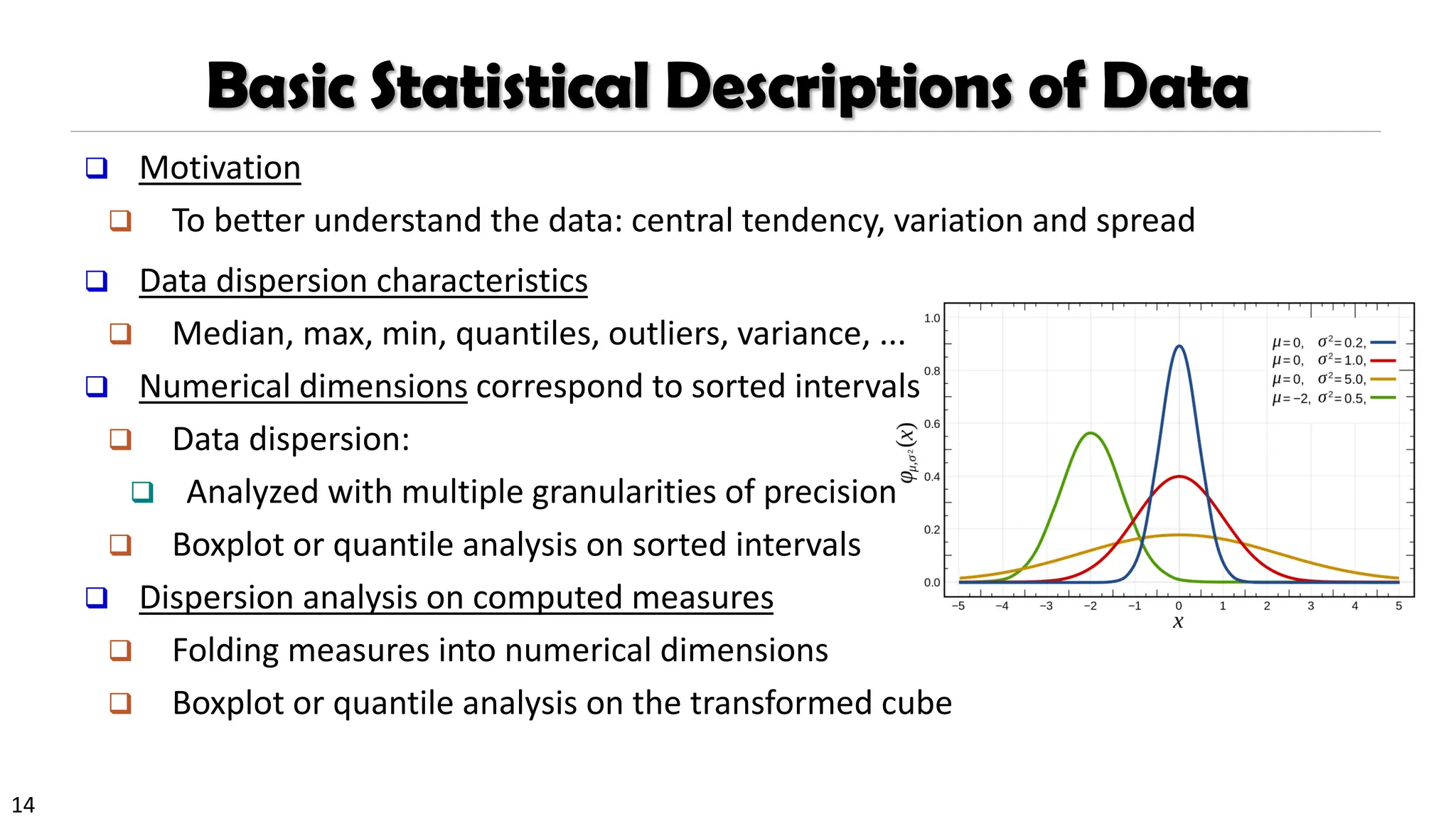
Basic Statistical Descriptions of Data
❑ Motivation
❑ To better understand the data: central tendency, variation and spread
❑ Data dispersion characteristics
❑ Median, max, min, quantiles, outliers, variance, ...
❑ Numerical dimensions correspond to sorted intervals
❑ Data dispersion:
❑ Analyzed with multiple granularities of precision
❑ Boxplot or quantile analysis on sorted intervals
❑ Dispersion analysis on computed measures
❑ Folding measures into numerical dimensions
❑ Boxplot or quantile analysis on the transformed cube

15
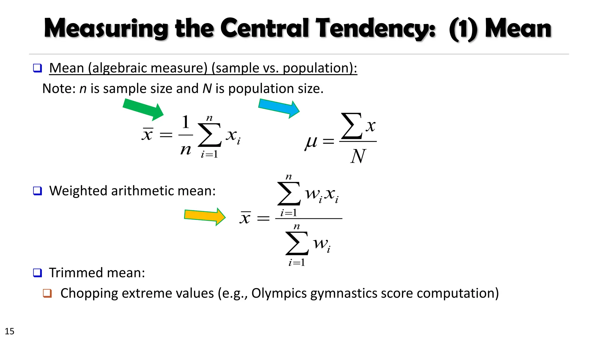
Measuring the Central Tendency: (1) Mean
❑ Mean (algebraic measure) (sample vs. population):
Note: n is sample size and N is population size.
❑ Weighted arithmetic mean:
❑ Trimmed mean:
❑ Chopping extreme values (e.g., Olympics gymnastics score computation)

=
=
n
i
i
x
n
x
1
1


=
=
= n
i
i
n
i
i
i
w
x
w
x
1
1
N
x

=


16
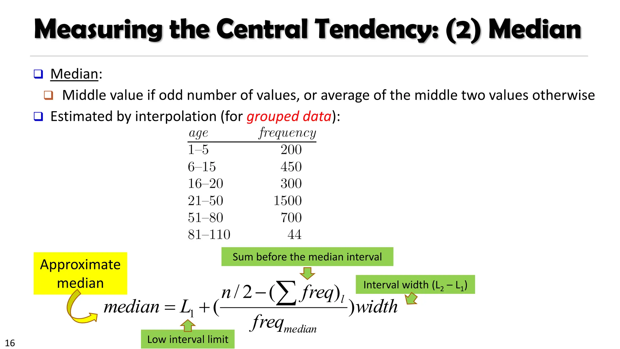
Measuring the Central Tendency: (2) Median
❑ Median:
❑ Middle value if odd number of values, or average of the middle two values otherwise
❑ Estimated by interpolation (for grouped data):
width
freq
freq
n
L
median
median
l
)
)
(
2
/
(
1

−
+
=
Approximate
median
Low interval limit
Interval width (L2 – L1)
Sum before the median interval

17
Measuring the Central Tendency: (3) Mode
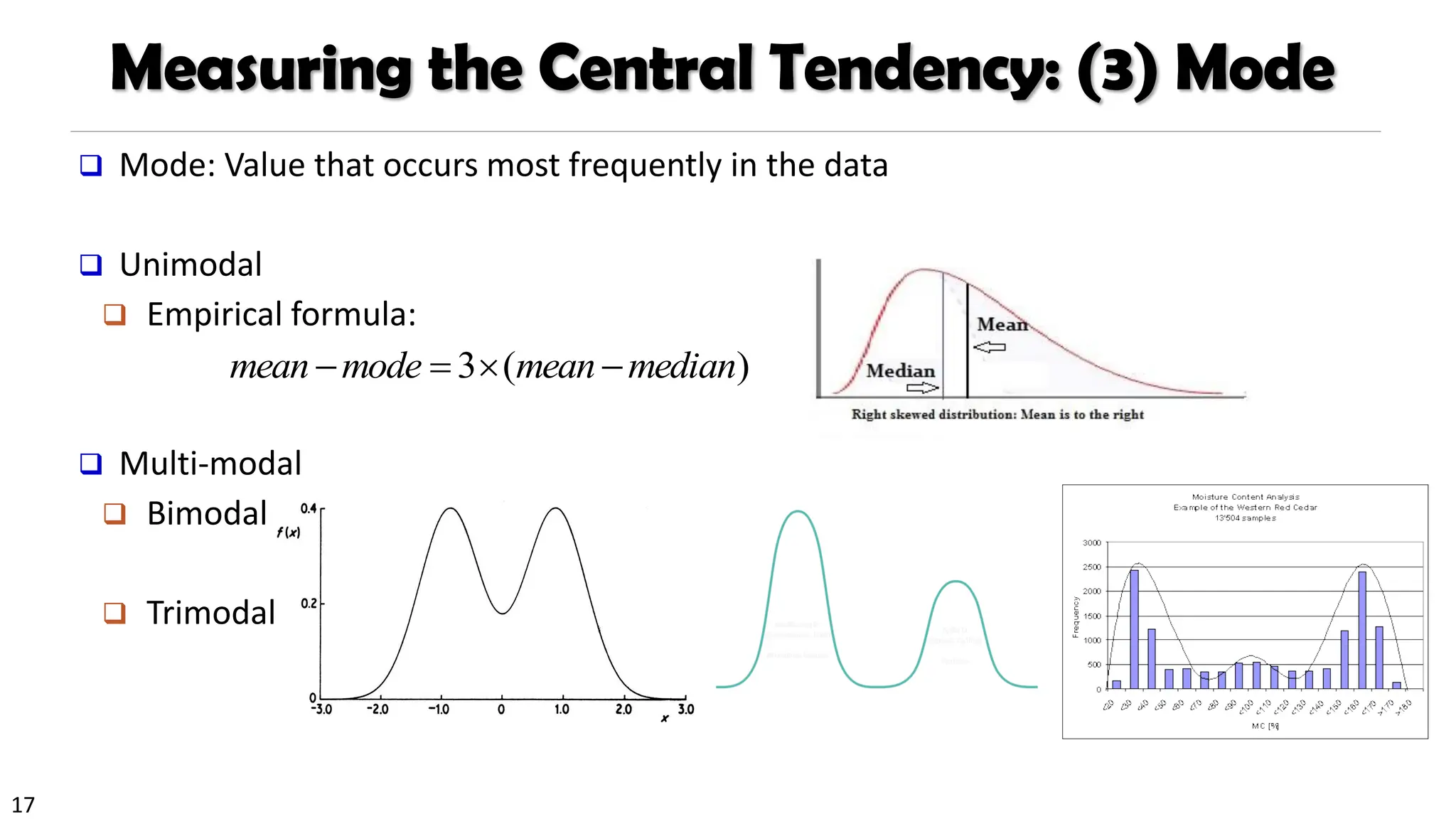
❑ Mode: Value that occurs most frequently in the data
❑ Unimodal
❑ Empirical formula:
❑ Multi-modal
❑ Bimodal
❑ Trimodal
)
(
3 median
mean
mode
mean −

=
−

18
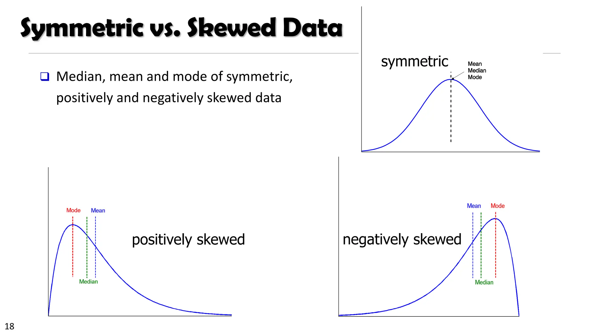
Symmetric vs. Skewed Data
❑ Median, mean and mode of symmetric,
positively and negatively skewed data
positively skewed negatively skewed
symmetric

19
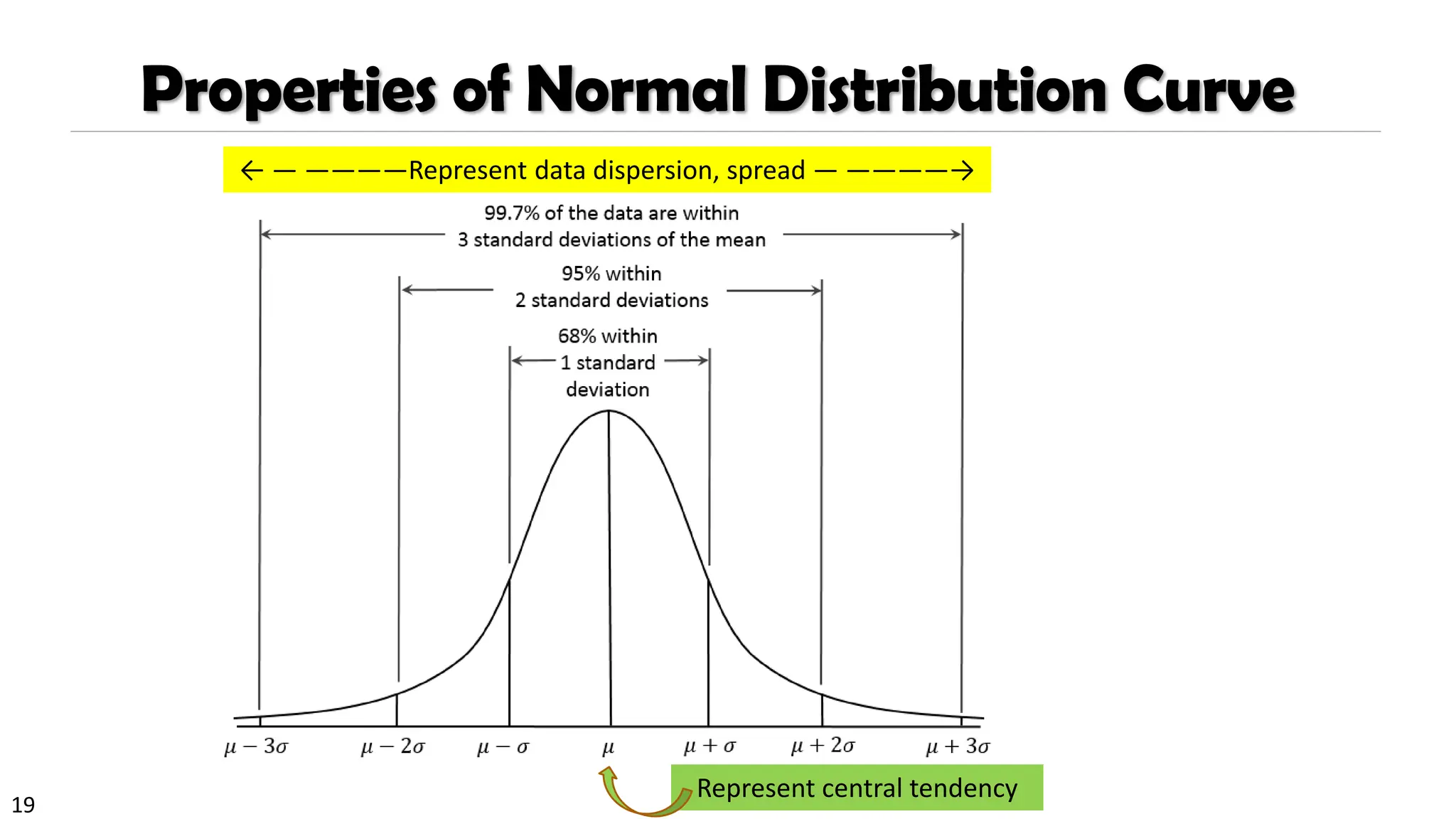
Properties of Normal Distribution Curve
← — ————Represent data dispersion, spread — ————→
Represent central tendency

20
Measures Data Distribution: Variance and Standard Deviation
❑ Variance and standard deviation (sample: s, population: σ)
❑ Variance: (algebraic, scalable computation)
❑ Q: Can you compute it incrementally and efficiently?
❑ Standard deviation s (or σ) is the square root of variance s2 (or σ2)
 
 = =
=
−
−
=
−
−
=
n
i
n
i
i
i
n
i
i x
n
x
n
x
x
n
s
1 1
2
2
1
2
2
]
)
(
1
[
1
1
)
(
1
1

 =
=
−
=
−
=
n
i
i
n
i
i x
N
x
N 1
2
2
1
2
2 1
)
(
1



Note: The subtle difference of
formulae for sample vs. population
• n : the size of the sample
• N : the size of the population

21
Correlation Analysis (for Categorical Data)
❑ Χ2 (chi-square) test:
❑ Null hypothesis: The two distributions are independent
❑ The cells that contribute the most to the Χ2 value are those whose actual count is
very different from the expected count
❑ The larger the Χ2 value, the more likely the variables are related
❑ Note: Correlation does not imply causality
❑ # of hospitals and # of car-theft in a city are correlated
❑ Both are causally linked to the third variable: population

22
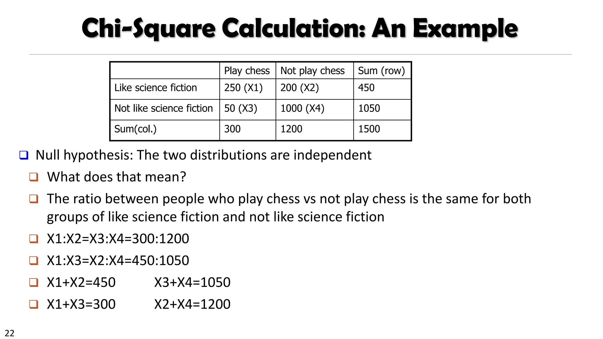
Chi-Square Calculation: An Example
Play chess Not play chess Sum (row)
Like science fiction 250 (X1) 200 (X2) 450
Not like science fiction 50 (X3) 1000 (X4) 1050
Sum(col.) 300 1200 1500
❑ Null hypothesis: The two distributions are independent
❑ What does that mean?
❑ The ratio between people who play chess vs not play chess is the same for both
groups of like science fiction and not like science fiction
❑ X1:X2=X3:X4=300:1200
❑ X1:X3=X2:X4=450:1050
❑ X1+X2=450 X3+X4=1050
❑ X1+X3=300 X2+X4=1200

23
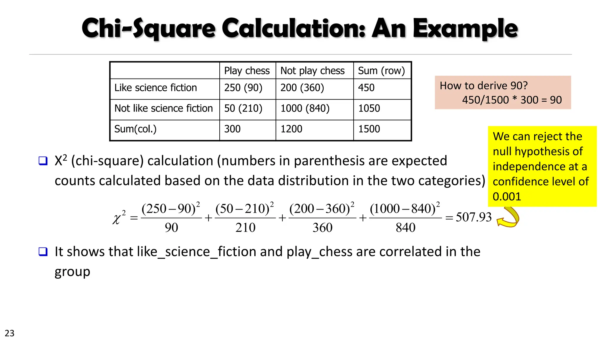
❑ Χ2 (chi-square) calculation (numbers in parenthesis are expected
counts calculated based on the data distribution in the two categories)
❑ It shows that like_science_fiction and play_chess are correlated in the
group
93
.
507
840
)
840
1000
(
360
)
360
200
(
210
)
210
50
(
90
)
90
250
( 2
2
2
2
2
=
−
+
−
+
−
+
−
=

Like science fiction 250 (90) 200 (360) 450
Not like science fiction 50 (210) 1000 (840) 1050
Sum(col.) 300 1200 1500
We can reject the
null hypothesis of
independence at a
confidence level of
0.001
How to derive 90?
450/1500 * 300 = 90

24
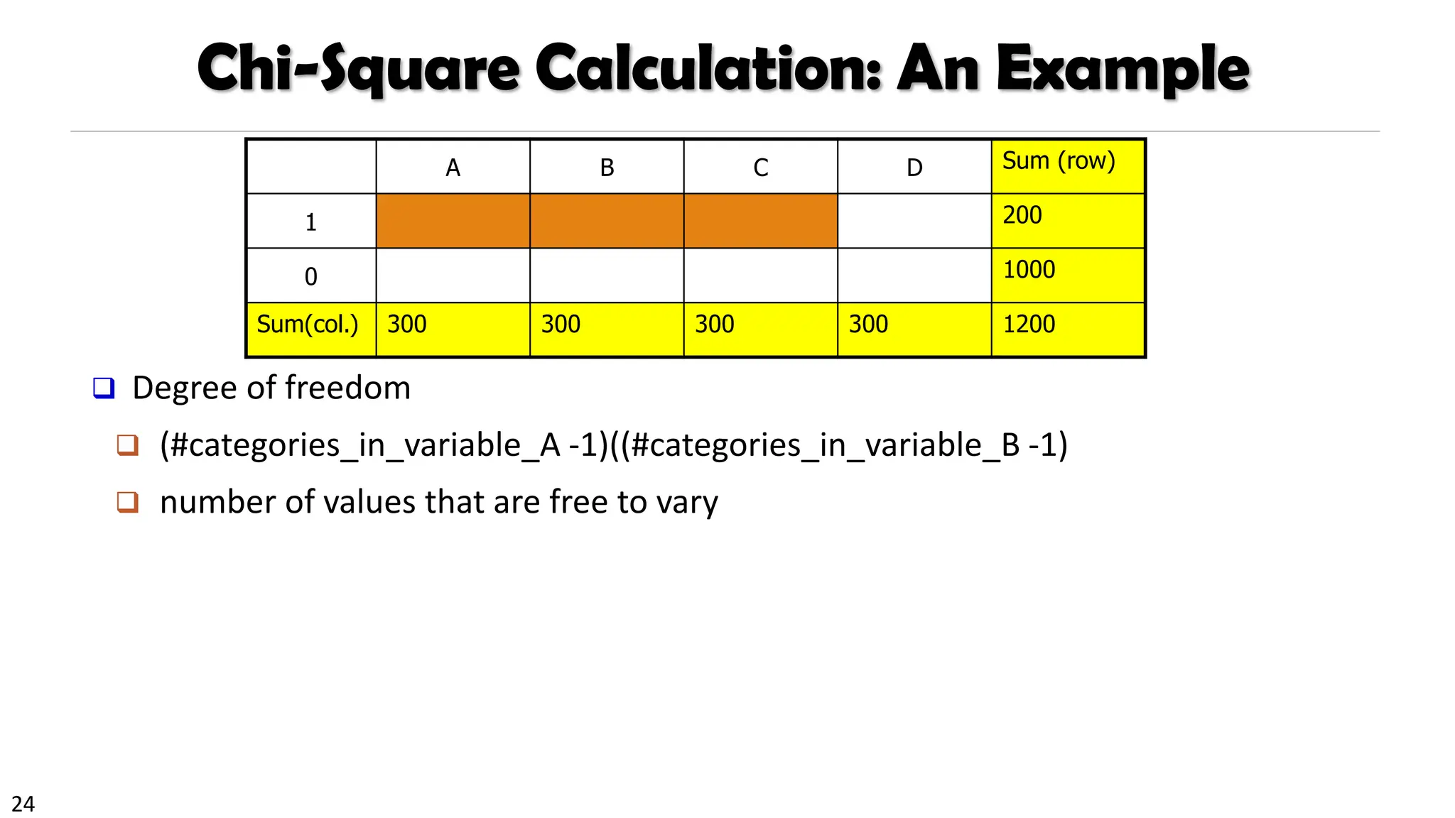
❑ Degree of freedom
❑ (#categories_in_variable_A -1)((#categories_in_variable_B -1)
❑ number of values that are free to vary
A B C D Sum (row)
1 200
0 1000
Sum(col.) 300 300 300 300 1200

25
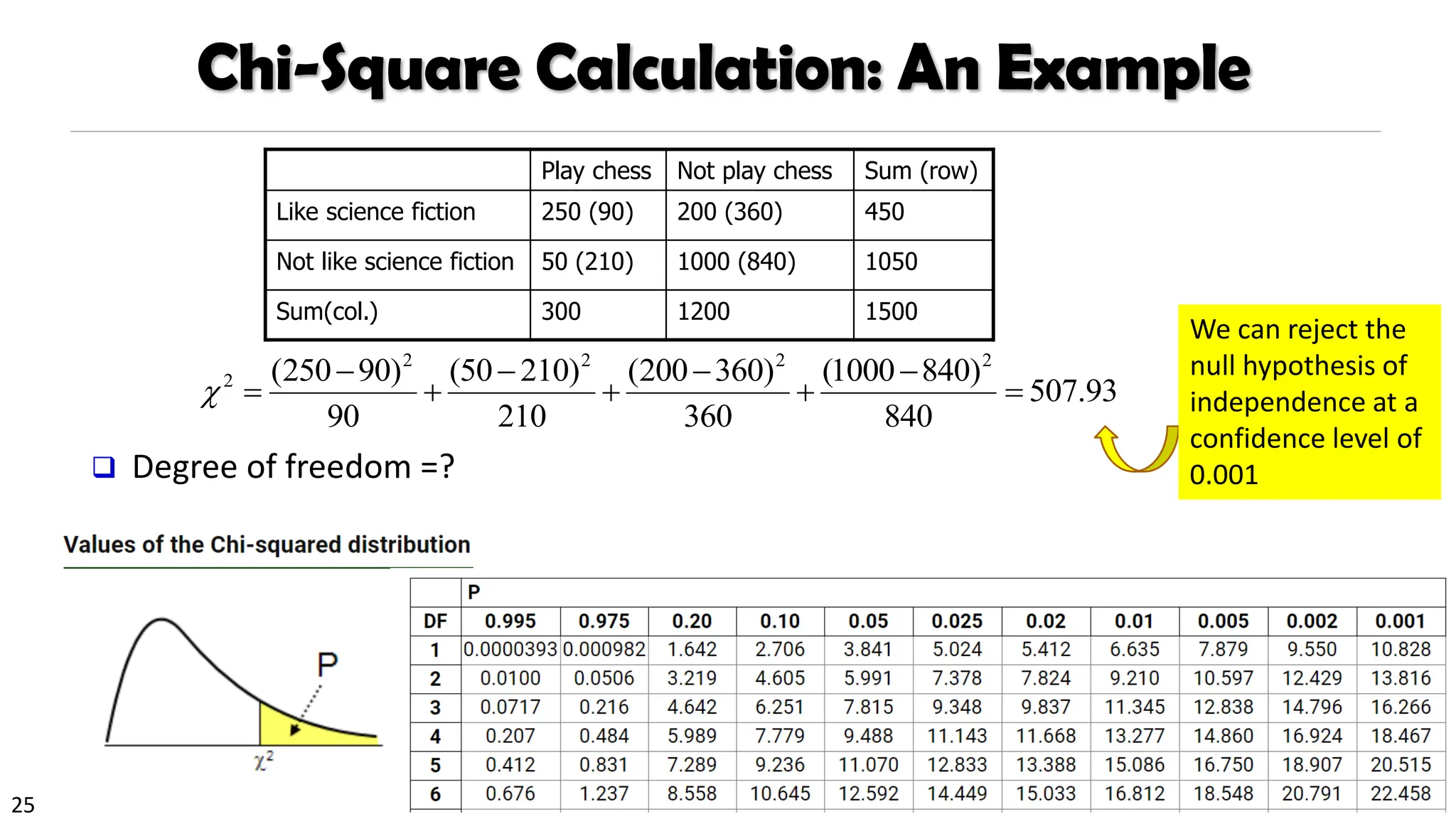
❑ Degree of freedom =?
93
.
507
840
)
840
1000
(
360
)
360
200
(
210
)
210
50
(
90
)
90
250
( 2
2
2
2
2
=
−
+
−
+
−
+
−
=

Like science fiction 250 (90) 200 (360) 450
Not like science fiction 50 (210) 1000 (840) 1050
Sum(col.) 300 1200 1500
We can reject the
null hypothesis of
independence at a
confidence level of
0.001

26
Variance for Single Variable (Numerical Data)
❑ The variance of a random variable X provides a measure of how much the value of
X deviates from the mean or expected value of X:
❑ where σ2 is the variance of X, σ is called standard deviation
µ is the mean, and µ = E[X] is the expected value of X
❑ That is, variance is the expected value of the square deviation from the mean
❑ It can also be written as:
❑ Sample variance
2
2 2
2
( ) ( ) if is discrete
var( ) [(X ) ]
( ) ( ) if is continuous
x
x f x X
X E
x f x dx X

 


−
 −


= = − = 
 −




2 2 2 2 2 2
var( ) [(X ) ] [X ] [X ] [ ( )]
X E E E E x
  
= = − = − = −
𝑠2 =
1
𝑛
෍
𝑖
𝑛
𝑥𝑖 − ො
𝜇 2 𝑠2 =
1
𝑛 − 1
෍
𝑖
𝑛
𝑥𝑖 − ො
𝜇 2

27
Covariance for Two Variables
❑ Covariance between two variables X1 and X2
where µ1 = E[X1] is the respective mean or expected value of X1; similarly for µ2
❑ Sample covariance between X1 and X2: ො
𝜎12 =
1
𝑛
σ𝑖=1
𝑛
𝑥𝑖1 − ෞ
𝜇1 𝑥𝑖2 − ෞ
𝜇2
❑ Sample covariance is a generalization of the sample variance:
ො
𝜎11 =
1
𝑛
෍
𝑖=1
𝑛
𝑥𝑖1 − ෞ
𝜇1 𝑥𝑖1 − ෞ
𝜇1
❑ Positive covariance: If σ12 > 0
❑ Negative covariance: If σ12 < 0
12 1 1 2 2 1 2 1 2 1 2 1 2
[( )( )] [ ] [ ] [ ] [ ]
E X X E X X E X X E X E X
    
= − − = − = −

28
Covariance for Two Variables
❑ Independence: If X1 and X2 are independent, σ12 = 0 but the reverse is not true
❑ Some pairs of random variables may have a covariance 0 but are not independent
❑ Only under some additional assumptions (e.g., the data follow multivariate normal
distributions) does a covariance of 0 imply independence
❑ Example:
E(𝑋1)=?
E(𝑋2)=?
E(𝑋1𝑋2)=?
𝑿𝟏 1 -1
𝑿𝟐 0 1 -1
12 1 1 2 2 1 2 1 2 1 2 1 2
[( )( )] [ ] [ ] [ ] [ ]
    
= − − = − = −

29
Example: Calculation of Covariance
❑ Suppose two stocks X1 and X2 have the following values in one week:
❑ (2, 5), (3, 8), (5, 10), (4, 11), (6, 14)
❑ Question: If the stocks are affected by the same industry trends, will their prices
rise or fall together?
❑ Covariance formula
❑ Its computation can be simplified as:
❑ E(X1) = (2 + 3 + 5 + 4 + 6)/ 5 = 20/5 = 4
❑ E(X2) = (5 + 8 + 10 + 11 + 14) /5 = 48/5 = 9.6
❑ σ12 = (2×5 + 3×8 + 5×10 + 4×11 + 6×14)/5 − 4 × 9.6 = 4
❑ Thus, X1 and X2 rise together since σ12 > 0
12 1 1 2 2 1 2 1 2 1 2 1 2
[( )( )] [ ] [ ] [ ] [ ]
    
= − − = − = −
12 1 2 1 2
[ ] [ ] [ ]
E X X E X E X
 = −

30
Correlation between Two Numerical Variables
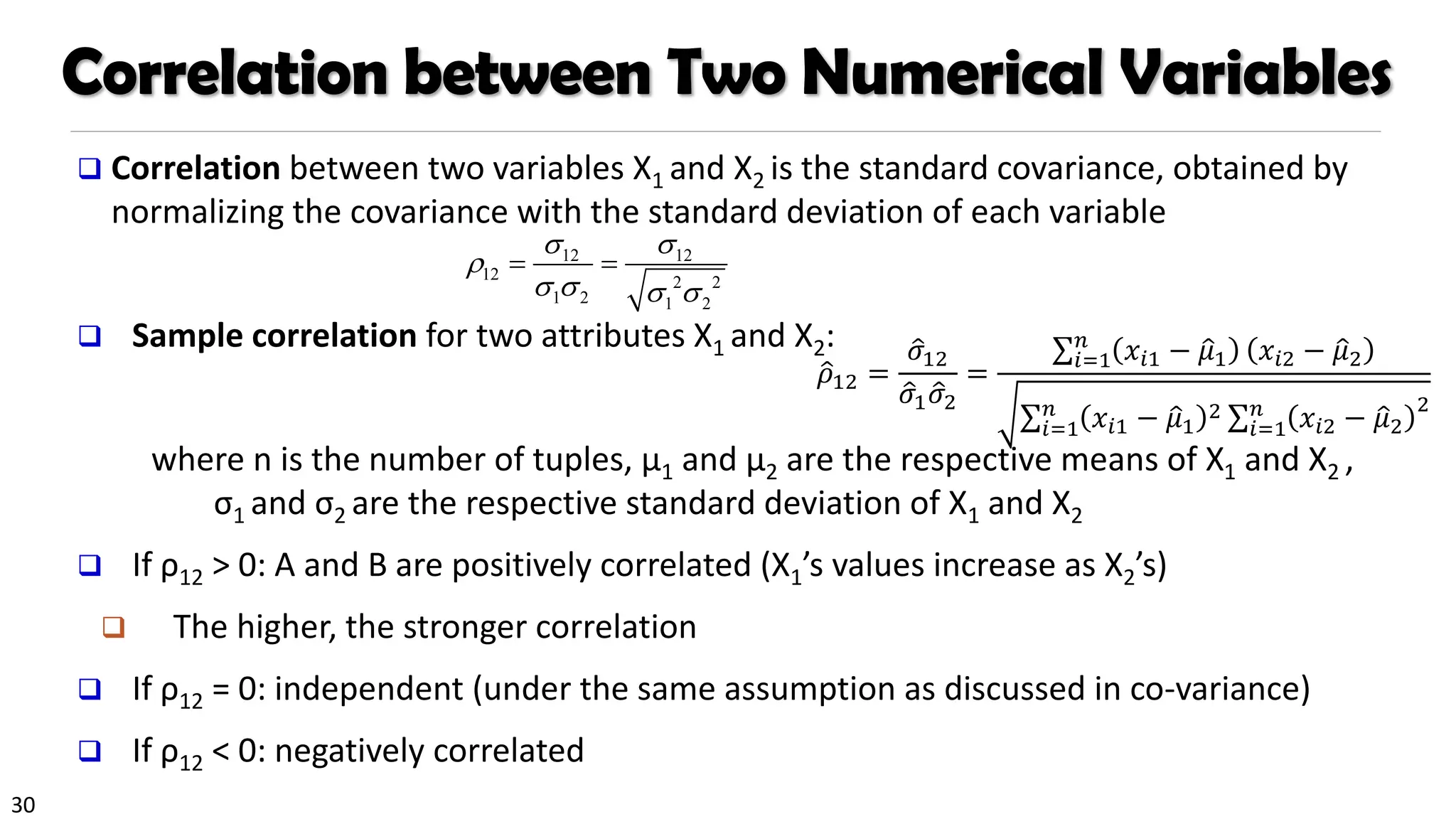
❑ Correlation between two variables X1 and X2 is the standard covariance, obtained by
normalizing the covariance with the standard deviation of each variable
❑ Sample correlation for two attributes X1 and X2:
where n is the number of tuples, µ1 and µ2 are the respective means of X1 and X2 ,
σ1 and σ2 are the respective standard deviation of X1 and X2
❑ If ρ12 > 0: A and B are positively correlated (X1’s values increase as X2’s)
❑ The higher, the stronger correlation
❑ If ρ12 = 0: independent (under the same assumption as discussed in co-variance)
❑ If ρ12 < 0: negatively correlated
12 12
12 2 2
1 2 1 2
 

   
= =
ො
𝜌12 =
ො
𝜎12
ො
𝜎1 ො
𝜎2
=
σ𝑖=1
𝑛
𝑥𝑖1 − ො
𝜇1 𝑥𝑖2 − ො
𝜇2
σ𝑖=1
𝑛
𝑥𝑖1 − ො
𝜇1
2 σ𝑖=1
𝑛
𝑥𝑖2 − ො
𝜇2
2

31
Visualizing Changes of Correlation Coefficient
❑ Correlation coefficient value range:
[–1, 1]
❑ A set of scatter plots shows sets of
points and their correlation
coefficients changing from –1 to 1

32
Covariance Matrix
❑ The variance and covariance information for the two variables X1 and X2
can be summarized as 2 X 2 covariance matrix as
❑ Generalizing it to d dimensions, we have,
1 1
1 1 2 2
2 2
[( )( ) ] [( )( )]
T
X
E E X X
X

   

−
 = − − = − −
−
X X
1 1 1 1 1 1 2 2
2 2 1 1 2 2 2 2
2
1 12
2
21 2
[( )( )] [( )( )]
[( )( )] [( )( )]
E X X E X X
E X X E X X
   
   
 
 
− − − −
 
=  
− − − −
 
 
=  
 

33
Graphic Displays of Basic Statistical Descriptions
❑ Boxplot: graphic display of five-number summary
❑ Histogram: x-axis are values, y-axis repres. frequencies
❑ Quantile plot: each value xi is paired with fi indicating that approximately 100 fi %
of data are  xi
❑ Quantile-quantile (q-q) plot: graphs the quantiles of one univariant distribution
against the corresponding quantiles of another
❑ Scatter plot: each pair of values is a pair of coordinates and plotted as points in the
plane

34
Measuring the Dispersion of Data: Quartiles & Boxplots
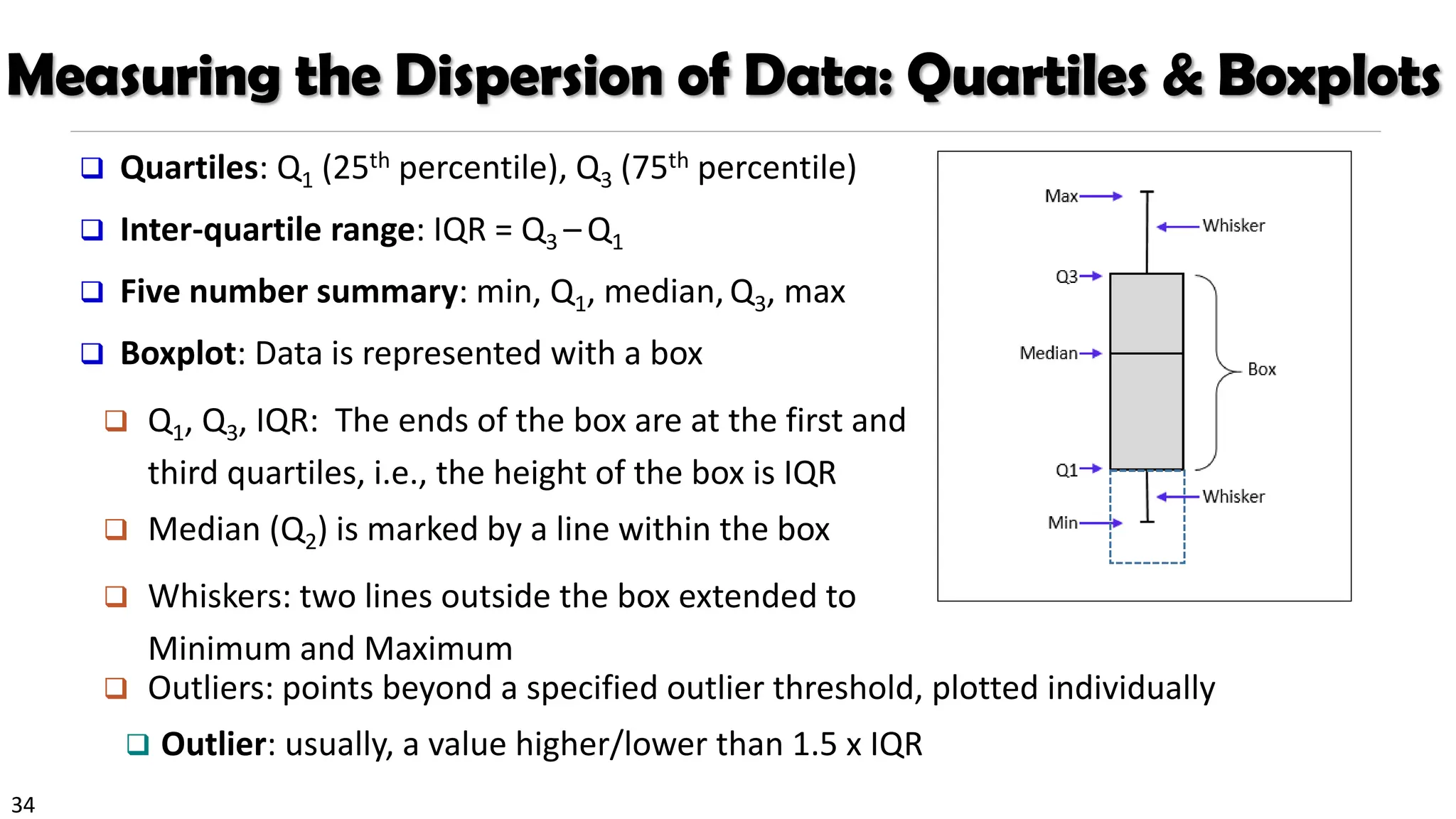
❑ Quartiles: Q1 (25th percentile), Q3 (75th percentile)
❑ Inter-quartile range: IQR = Q3 – Q1
❑ Five number summary: min, Q1, median, Q3, max
❑ Boxplot: Data is represented with a box
❑ Q1, Q3, IQR: The ends of the box are at the first and
third quartiles, i.e., the height of the box is IQR
❑ Median (Q2) is marked by a line within the box
❑ Whiskers: two lines outside the box extended to
Minimum and Maximum
❑ Outliers: points beyond a specified outlier threshold, plotted individually
❑ Outlier: usually, a value higher/lower than 1.5 x IQR

35
0
5
10
15
20
25
30
35
40
10000 30000 50000 70000 90000
Histogram Analysis
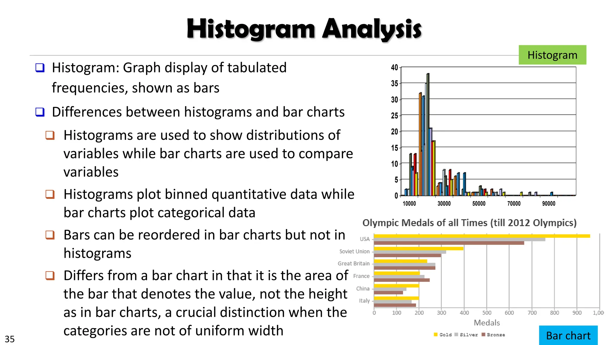
❑ Histogram: Graph display of tabulated
frequencies, shown as bars
❑ Differences between histograms and bar charts
❑ Histograms are used to show distributions of
variables while bar charts are used to compare
variables
❑ Histograms plot binned quantitative data while
bar charts plot categorical data
❑ Bars can be reordered in bar charts but not in
histograms
❑ Differs from a bar chart in that it is the area of
the bar that denotes the value, not the height
as in bar charts, a crucial distinction when the
categories are not of uniform width
Histogram
Bar chart

36
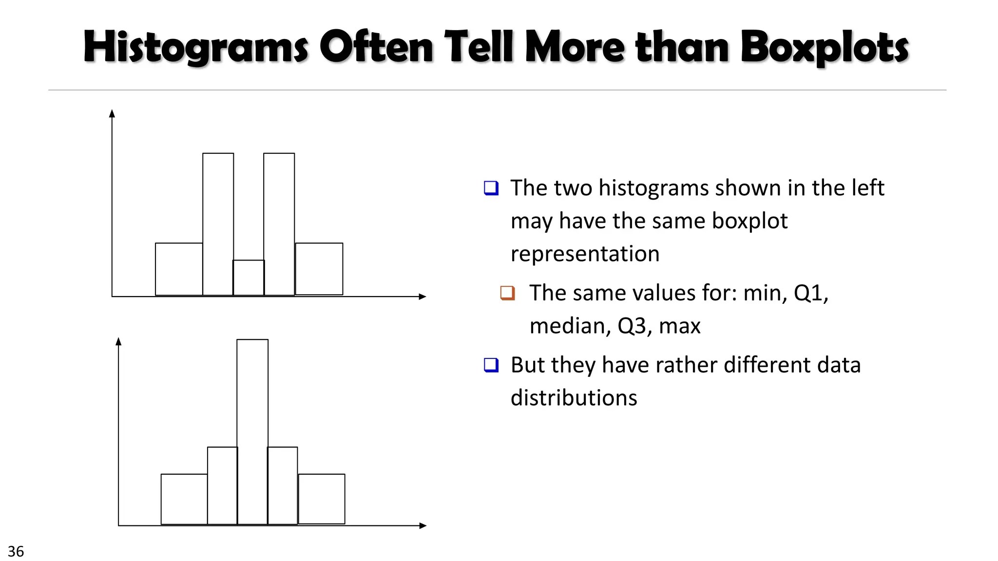
Histograms Often Tell More than Boxplots
❑ The two histograms shown in the left
may have the same boxplot
representation
❑ The same values for: min, Q1,
median, Q3, max
❑ But they have rather different data
distributions

37 Data Mining: Concepts and Techniques
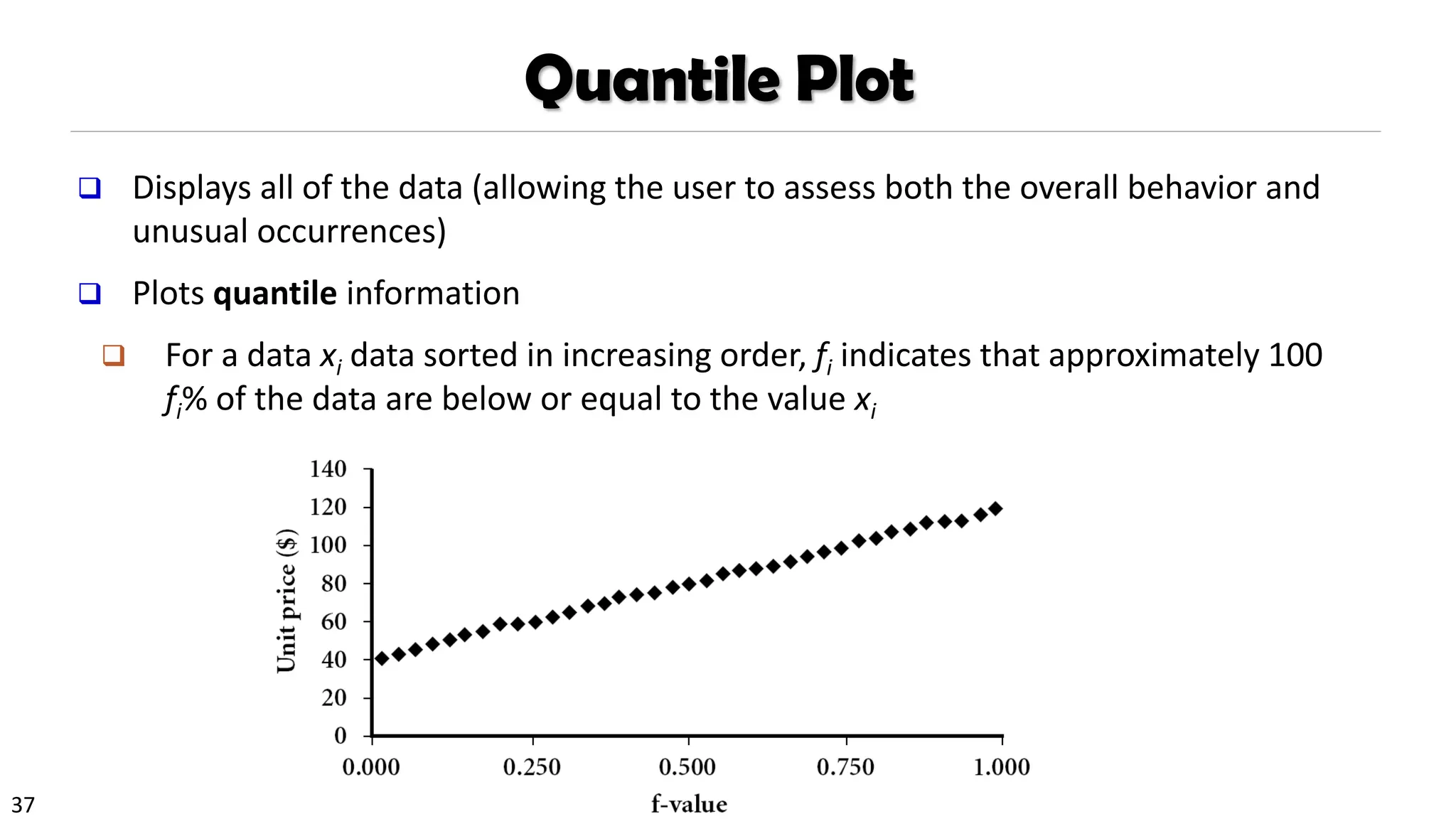
Quantile Plot
❑ Displays all of the data (allowing the user to assess both the overall behavior and
unusual occurrences)
❑ Plots quantile information
❑ For a data xi data sorted in increasing order, fi indicates that approximately 100
fi% of the data are below or equal to the value xi

38
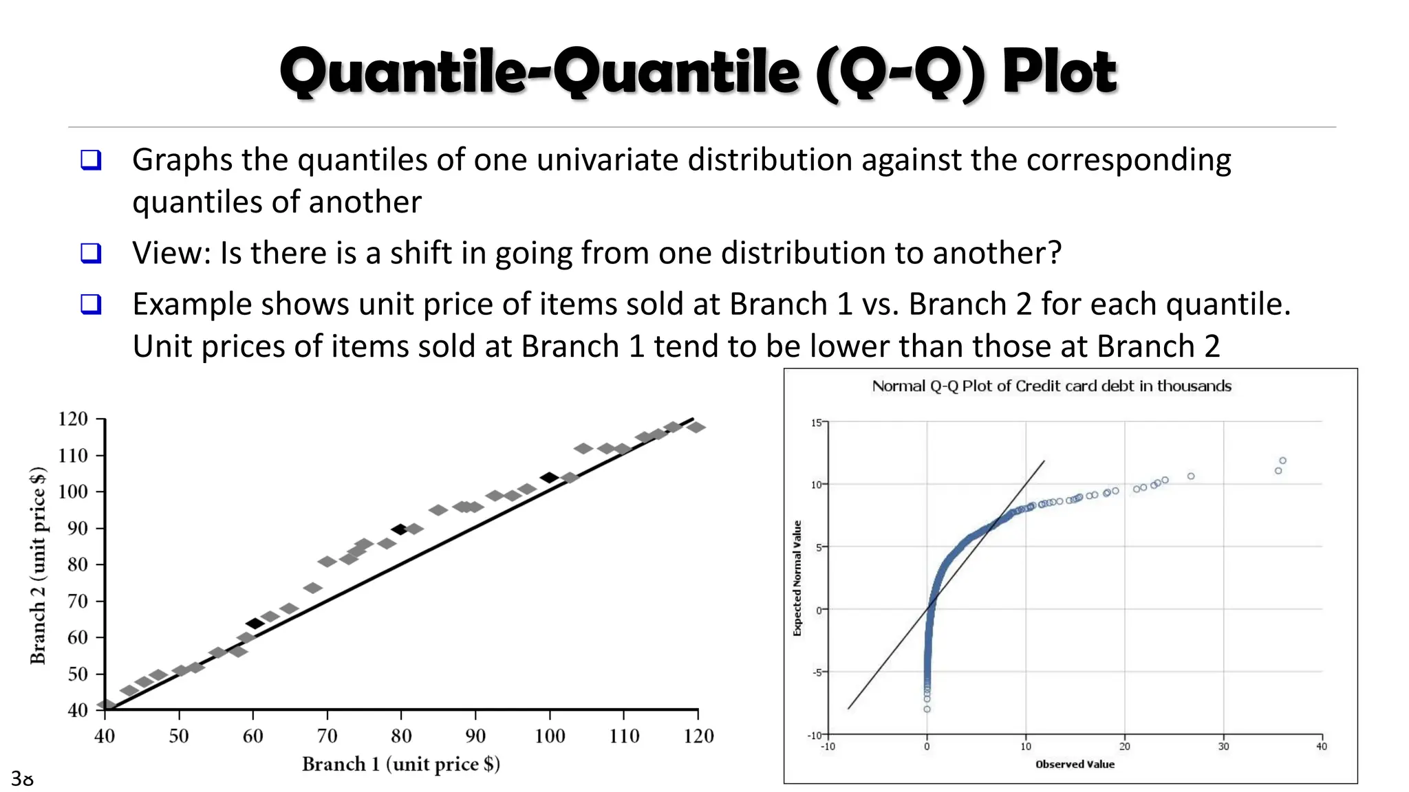
Quantile-Quantile (Q-Q) Plot
❑ Graphs the quantiles of one univariate distribution against the corresponding
quantiles of another
❑ View: Is there is a shift in going from one distribution to another?
❑ Example shows unit price of items sold at Branch 1 vs. Branch 2 for each quantile.
Unit prices of items sold at Branch 1 tend to be lower than those at Branch 2

39
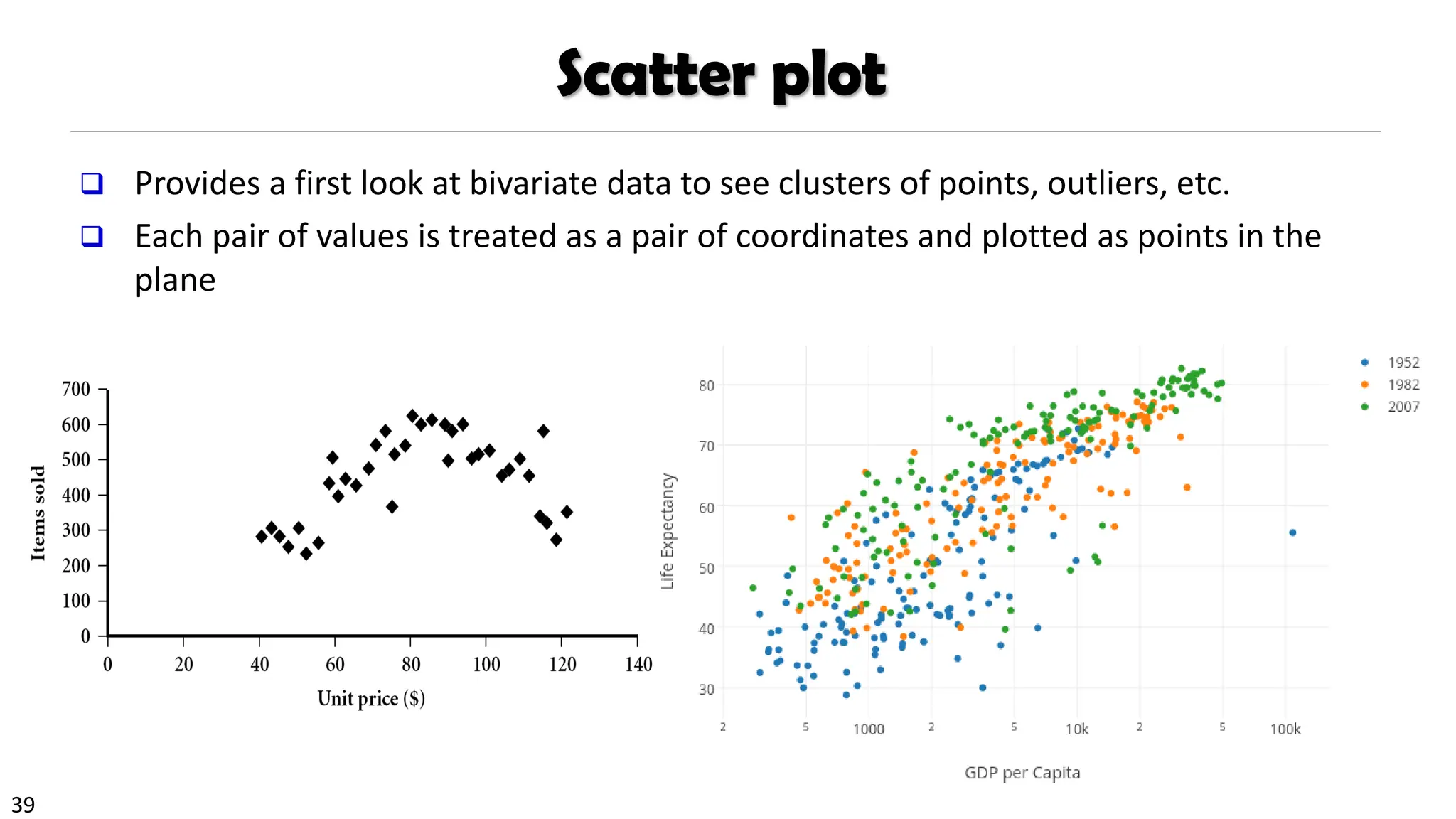
Scatter plot
❑ Provides a first look at bivariate data to see clusters of points, outliers, etc.
❑ Each pair of values is treated as a pair of coordinates and plotted as points in the
plane

40
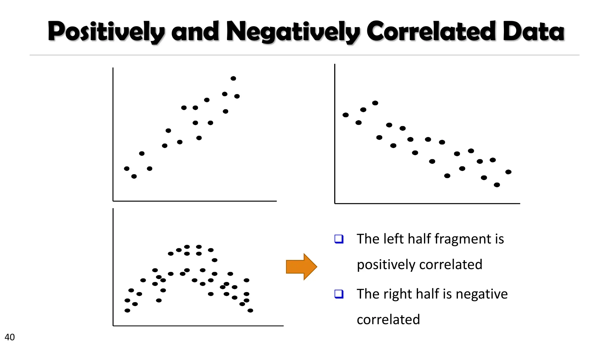
Positively and Negatively Correlated Data
❑ The left half fragment is
positively correlated
❑ The right half is negative
correlated

42
Similarity and Distance Measures
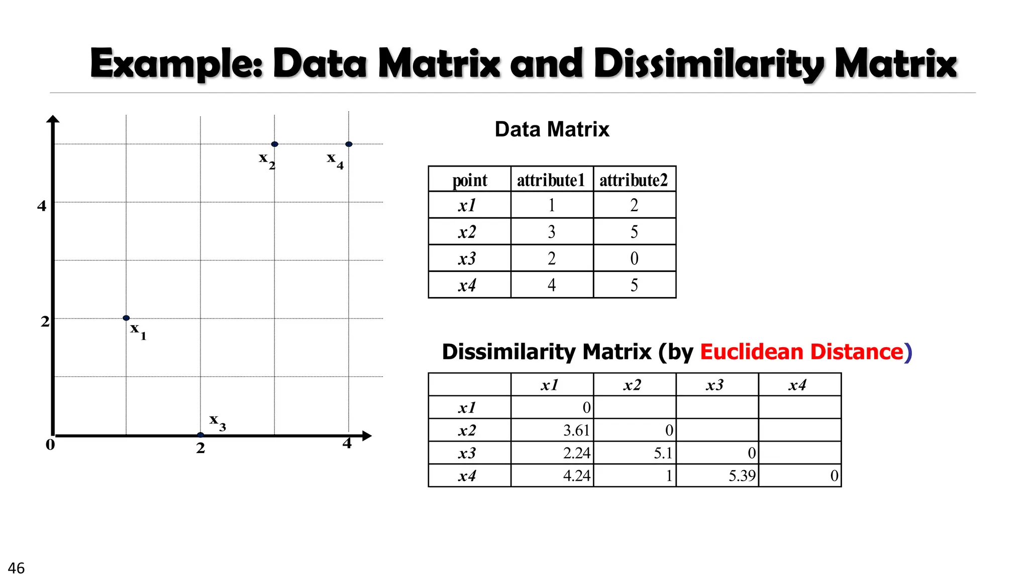
❑ Data Matrix versus Dissimilarity Matrix
❑ Proximity Measures for Nominal Attributes
❑ Proximity Measures for Binary Attributes
❑ Dissimilarity of Numeric Data: Minkowski Distance
❑ Proximity Measures for Ordinal Attributes
❑ Dissimilarity for Attributes of Mixed Types
❑ Cosine Similarity
❑ Capturing Hidden Semantics in Similarity Measures

43
Similarity, Dissimilarity, and Proximity
❑ Similarity measure or similarity function
❑ A real-valued function that quantifies the similarity between two objects
❑ Measure how two data objects are alike: The higher value, the more alike
❑ Often falls in the range [0,1]: 0: no similarity; 1: completely similar
❑ Dissimilarity (or distance) measure
❑ Numerical measure of how different two data objects are
❑ In some sense, the inverse of similarity: The lower, the more alike
❑ Minimum dissimilarity is often 0 (i.e., completely similar)
❑ Range [0, 1] or [0, ∞) , depending on the definition
❑ Proximity usually refers to either similarity or dissimilarity

44
Data Matrix and Dissimilarity Matrix
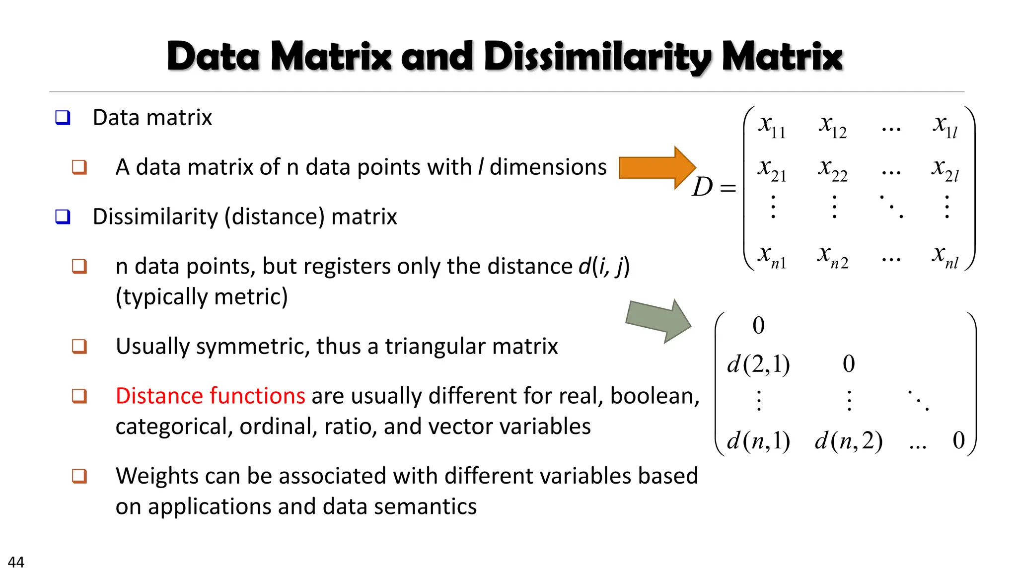
❑ Data matrix
❑ A data matrix of n data points with l dimensions
❑ Dissimilarity (distance) matrix
❑ n data points, but registers only the distance d(i, j)
(typically metric)
❑ Usually symmetric, thus a triangular matrix
❑ Distance functions are usually different for real, boolean,
categorical, ordinal, ratio, and vector variables
❑ Weights can be associated with different variables based
on applications and data semantics
11 12 1
21 22 2
1 2
...
...
...
l
l
n n nl
x x x
x x x
D
x x x
 
 
 
=
 
 
 
0
(2,1) 0
( ,1) ( ,2) ... 0
d
d n d n
 
 
 
 
 
 

45
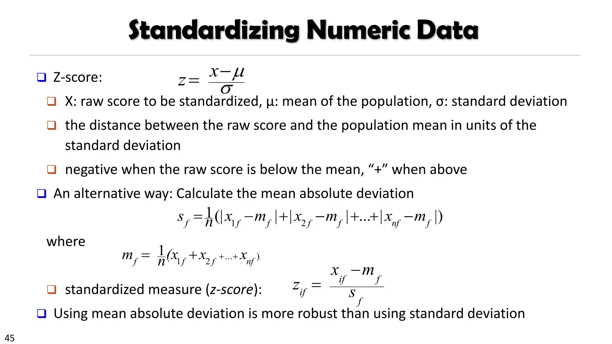
Standardizing Numeric Data
❑ Z-score:
❑ X: raw score to be standardized, μ: mean of the population, σ: standard deviation
❑ the distance between the raw score and the population mean in units of the
standard deviation
❑ negative when the raw score is below the mean, “+” when above
❑ An alternative way: Calculate the mean absolute deviation
where
❑ standardized measure (z-score):
❑ Using mean absolute deviation is more robust than using standard deviation
.
)
...
2
1
1
nf
f
f
f
x
x
(x
n
m +
+
+
=
|)
|
...
|
|
|
(|
1
2
1 f
nf
f
f
f
f
f
m
x
m
x
m
x
n
s −
+
+
−
+
−
=
f
f
if
if s
m
x
z
−
=


−
= x
z

46
Example: Data Matrix and Dissimilarity Matrix
point attribute1 attribute2
x1 1 2
x2 3 5
x3 2 0
x4 4 5
Dissimilarity Matrix (by Euclidean Distance)
x1 x2 x3 x4
x1 0
x2 3.61 0
x3 2.24 5.1 0
x4 4.24 1 5.39 0
Data Matrix

47
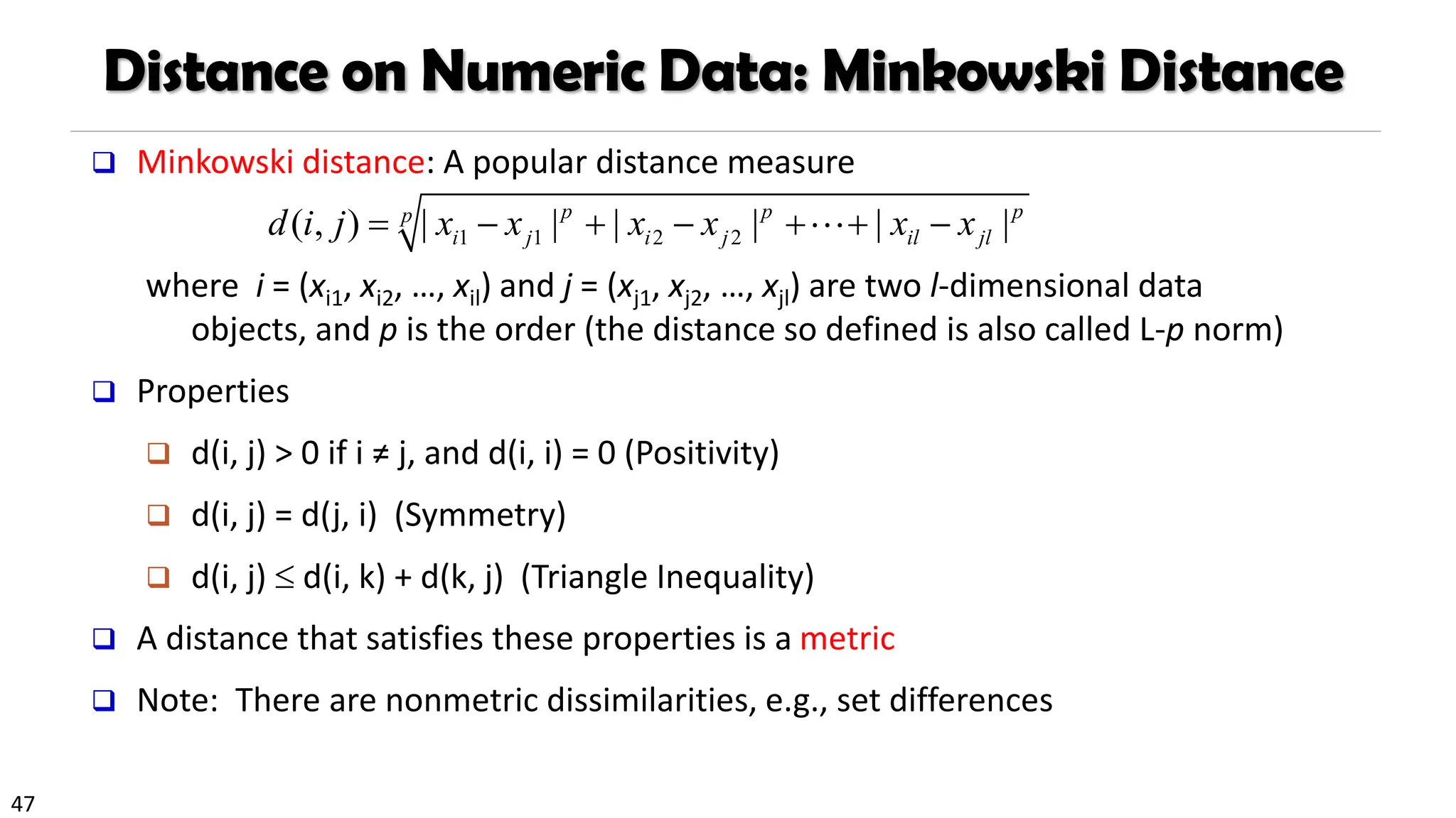
Distance on Numeric Data: Minkowski Distance
❑ Minkowski distance: A popular distance measure
where i = (xi1, xi2, …, xil) and j = (xj1, xj2, …, xjl) are two l-dimensional data
objects, and p is the order (the distance so defined is also called L-p norm)
❑ Properties
❑ d(i, j) > 0 if i ≠ j, and d(i, i) = 0 (Positivity)
❑ d(i, j) = d(j, i) (Symmetry)
❑ d(i, j)  d(i, k) + d(k, j) (Triangle Inequality)
❑ A distance that satisfies these properties is a metric
❑ Note: There are nonmetric dissimilarities, e.g., set differences
1 1 2 2
( , ) | | | | | |
p p p
p
i j i j il jl
d i j x x x x x x
= − + − + + −

48
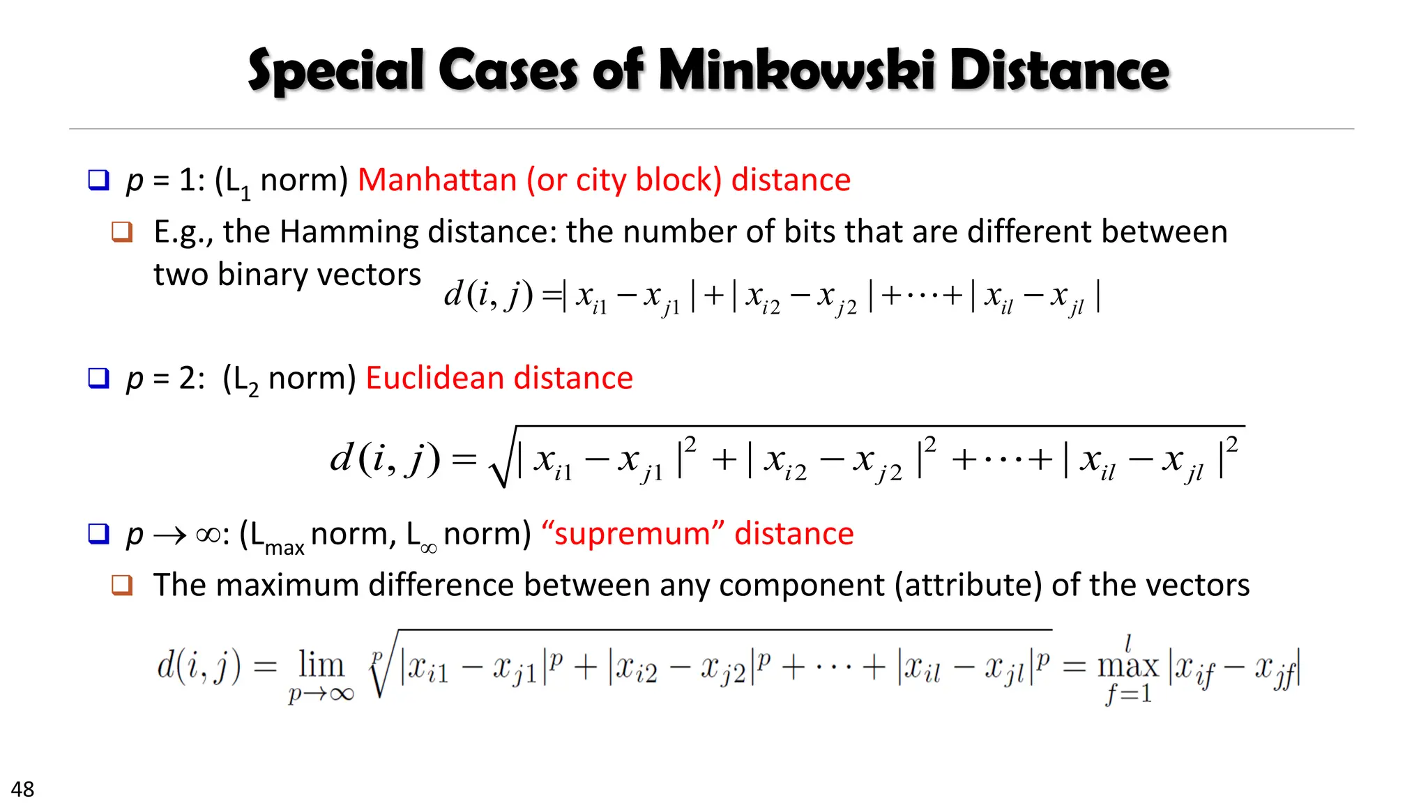
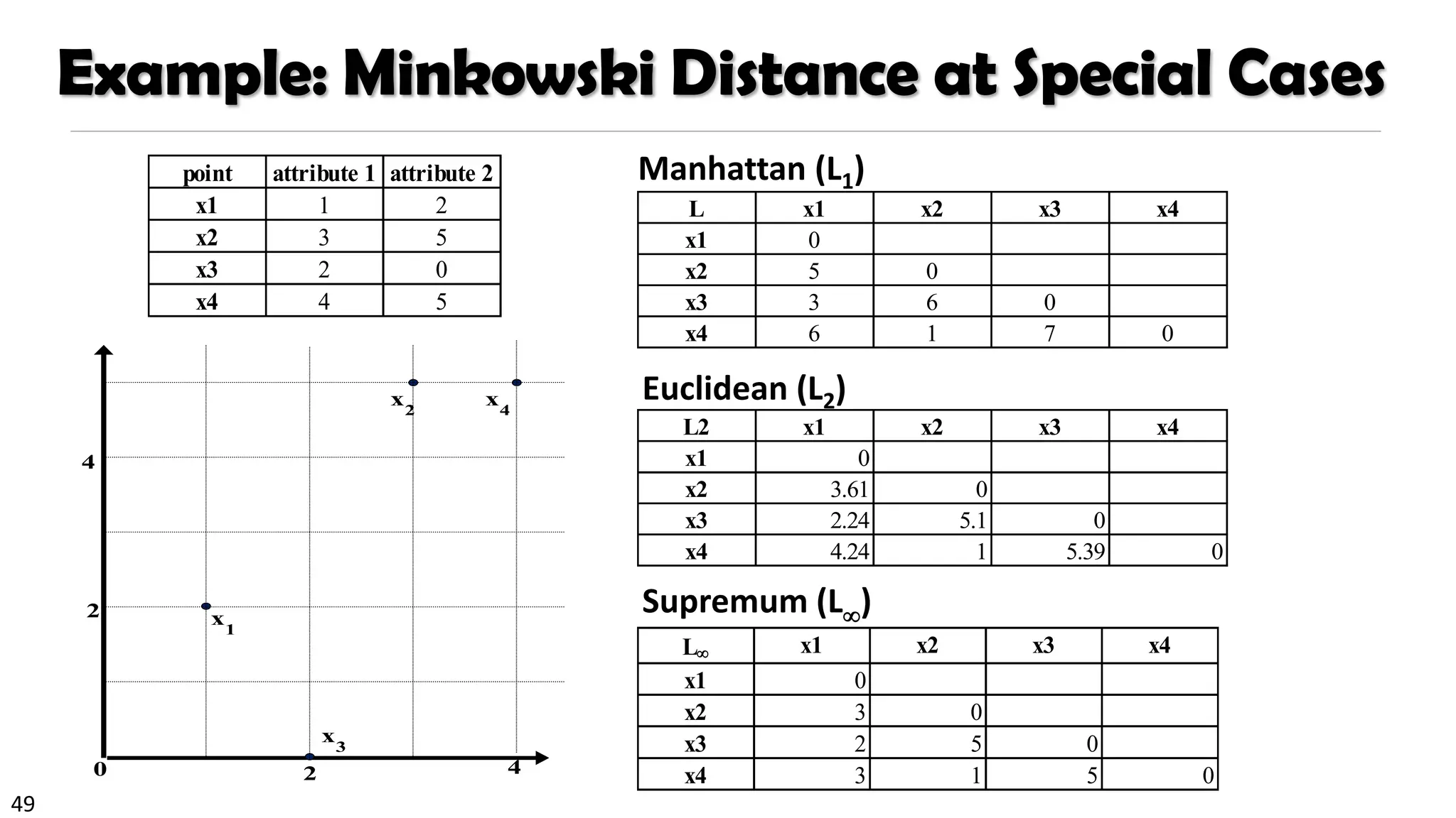
Special Cases of Minkowski Distance
❑ p = 1: (L1 norm) Manhattan (or city block) distance
❑ E.g., the Hamming distance: the number of bits that are different between
two binary vectors
❑ p = 2: (L2 norm) Euclidean distance
❑ p → : (Lmax norm, L norm) “supremum” distance
❑ The maximum difference between any component (attribute) of the vectors
1 1 2 2
( , ) | | | | | |
i j i j il jl
d i j x x x x x x
= − + − + + −
2 2 2
1 1 2 2
( , ) | | | | | |
i j i j il jl
d i j x x x x x x
= − + − + + −

49
Example: Minkowski Distance at Special Cases
point attribute 1 attribute 2
x1 1 2
x2 3 5
x3 2 0
x4 4 5
L x1 x2 x3 x4
x1 0
x2 5 0
x3 3 6 0
x4 6 1 7 0
L2 x1 x2 x3 x4
x1 0
x2 3.61 0
x3 2.24 5.1 0
x4 4.24 1 5.39 0
L x1 x2 x3 x4
x1 0
x2 3 0
x3 2 5 0
x4 3 1 5 0
Manhattan (L1)
Euclidean (L2)
Supremum (L)

50
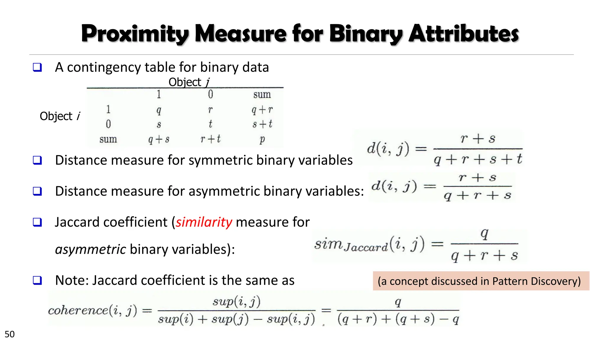
Proximity Measure for Binary Attributes
❑ A contingency table for binary data
❑ Distance measure for symmetric binary variables:
❑ Distance measure for asymmetric binary variables:
❑ Jaccard coefficient (similarity measure for
asymmetric binary variables):
❑ Note: Jaccard coefficient is the same as
“coherence”:
Object i
Object j
(a concept discussed in Pattern Discovery)

51
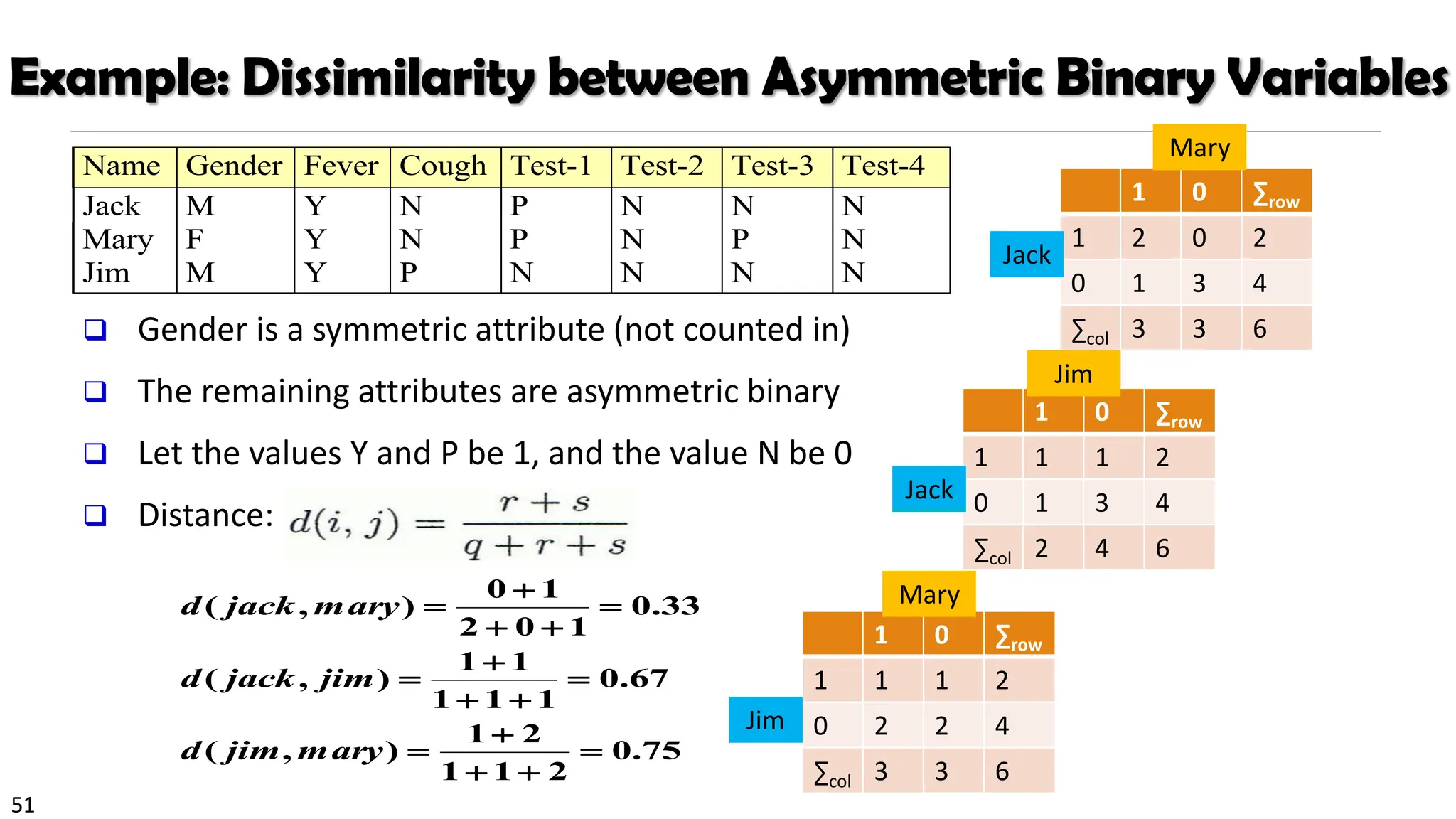
Example: Dissimilarity between Asymmetric Binary Variables
❑ Gender is a symmetric attribute (not counted in)
❑ The remaining attributes are asymmetric binary
❑ Let the values Y and P be 1, and the value N be 0
❑ Distance:
Name Gender Fever Cough Test-1 Test-2 Test-3 Test-4
Jack M Y N P N N N
Mary F Y N P N P N
Jim M Y P N N N N
75
.
0
2
1
1
2
1
)
,
(
67
.
0
1
1
1
1
1
)
,
(
33
.
0
1
0
2
1
0
)
,
(
=
+
+
+
=
=
+
+
+
=
=
+
+
+
=
mary
jim
d
jim
jack
d
mary
jack
d
1 0 ∑row
1 2 0 2
0 1 3 4
∑col 3 3 6
Jack
Mary
1 0 ∑row
1 1 1 2
0 1 3 4
∑col 2 4 6
Jim
1 0 ∑row
1 1 1 2
0 2 2 4
∑col 3 3 6
Jim
Mary
Jack

52
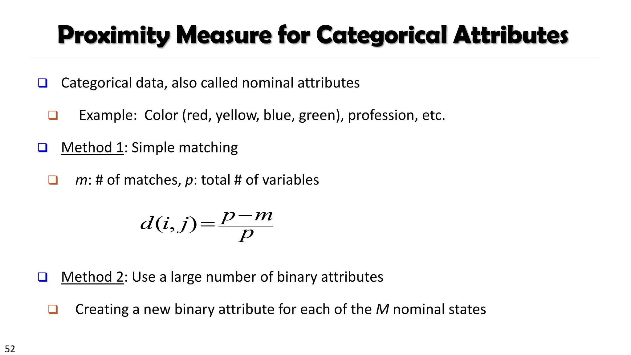
Proximity Measure for Categorical Attributes
❑ Categorical data, also called nominal attributes
❑ Example: Color (red, yellow, blue, green), profession, etc.
❑ Method 1: Simple matching
❑ m: # of matches, p: total # of variables
❑ Method 2: Use a large number of binary attributes
❑ Creating a new binary attribute for each of the M nominal states
p
m
p
j
i
d −
=
)
,
(

53
Ordinal Variables
❑ An ordinal variable can be discrete or continuous
❑ Order is important, e.g., rank (e.g., freshman, sophomore, junior, senior)
❑ Can be treated like interval-scaled
❑ Replace an ordinal variable value by its rank:
❑ Map the range of each variable onto [0, 1] by replacing i-th object in
the f-th variable by
❑ Example: freshman: 0; sophomore: 1/3; junior: 2/3; senior 1
❑ Then distance: d(freshman, senior) = 1, d(junior, senior) = 1/3
❑ Compute the dissimilarity using methods for interval-scaled variables
1
1
if
if
f
r
z
M
−
=
−
{1,..., }
if f
r M


54
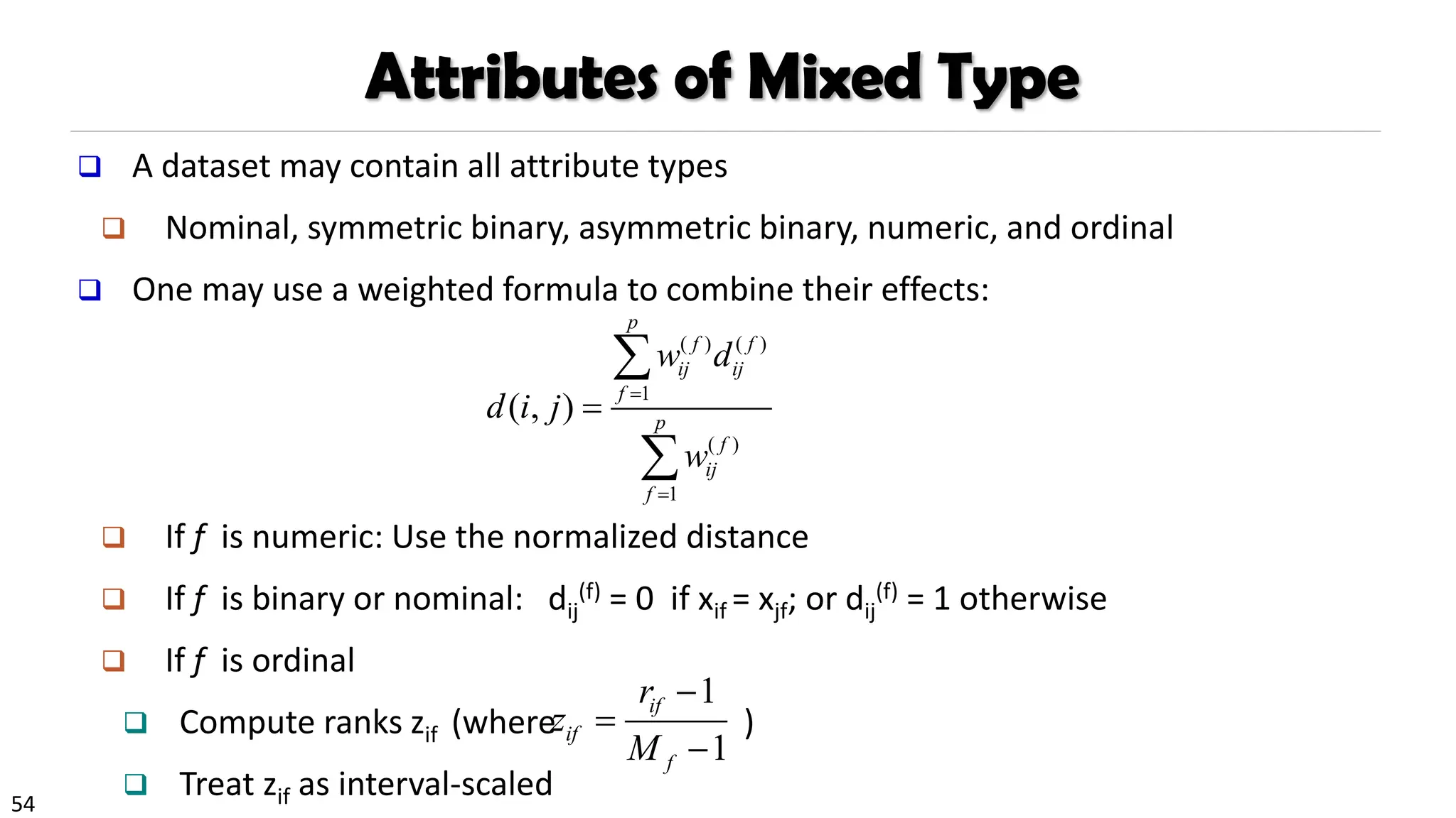
Attributes of Mixed Type
❑ A dataset may contain all attribute types
❑ Nominal, symmetric binary, asymmetric binary, numeric, and ordinal
❑ One may use a weighted formula to combine their effects:
❑ If f is numeric: Use the normalized distance
❑ If f is binary or nominal: dij
(f) = 0 if xif = xjf; or dij
(f) = 1 otherwise
❑ If f is ordinal
❑ Compute ranks zif (where )
❑ Treat zif as interval-scaled
1
1
if
if
f
r
z
M
−
=
−
( ) ( )
1
( )
1
( , )
p
f f
ij ij
f
p
f
ij
f
w d
d i j
w
=
=
=



55
Cosine Similarity of Two Vectors
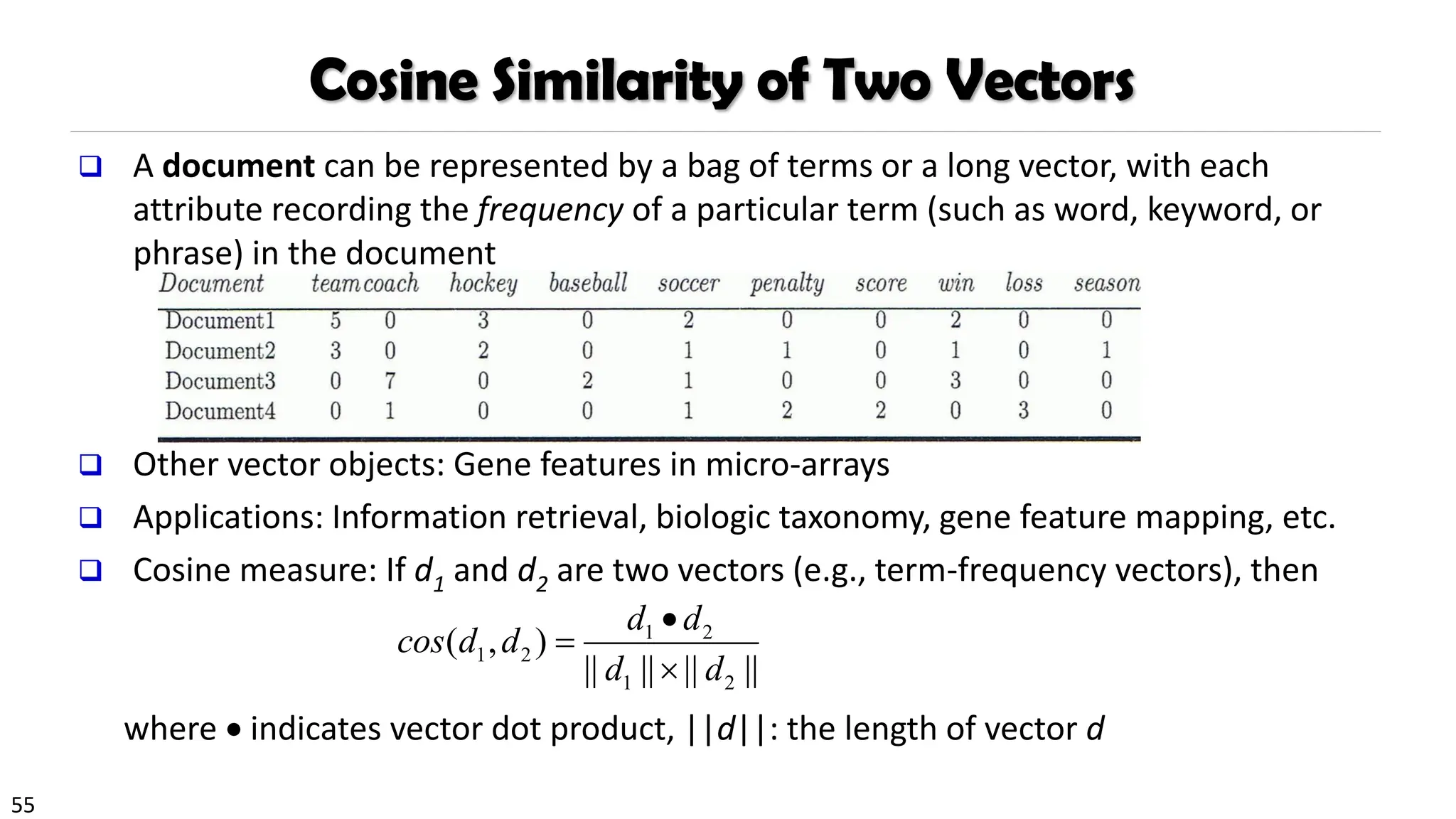
❑ A document can be represented by a bag of terms or a long vector, with each
attribute recording the frequency of a particular term (such as word, keyword, or
phrase) in the document
❑ Other vector objects: Gene features in micro-arrays
❑ Applications: Information retrieval, biologic taxonomy, gene feature mapping, etc.
❑ Cosine measure: If d1 and d2 are two vectors (e.g., term-frequency vectors), then
where • indicates vector dot product, ||d||: the length of vector d
1 2
1 2
1 2
( , )
|| || || ||
d d
cos d d
d d
•
=


56
Example: Calculating Cosine Similarity
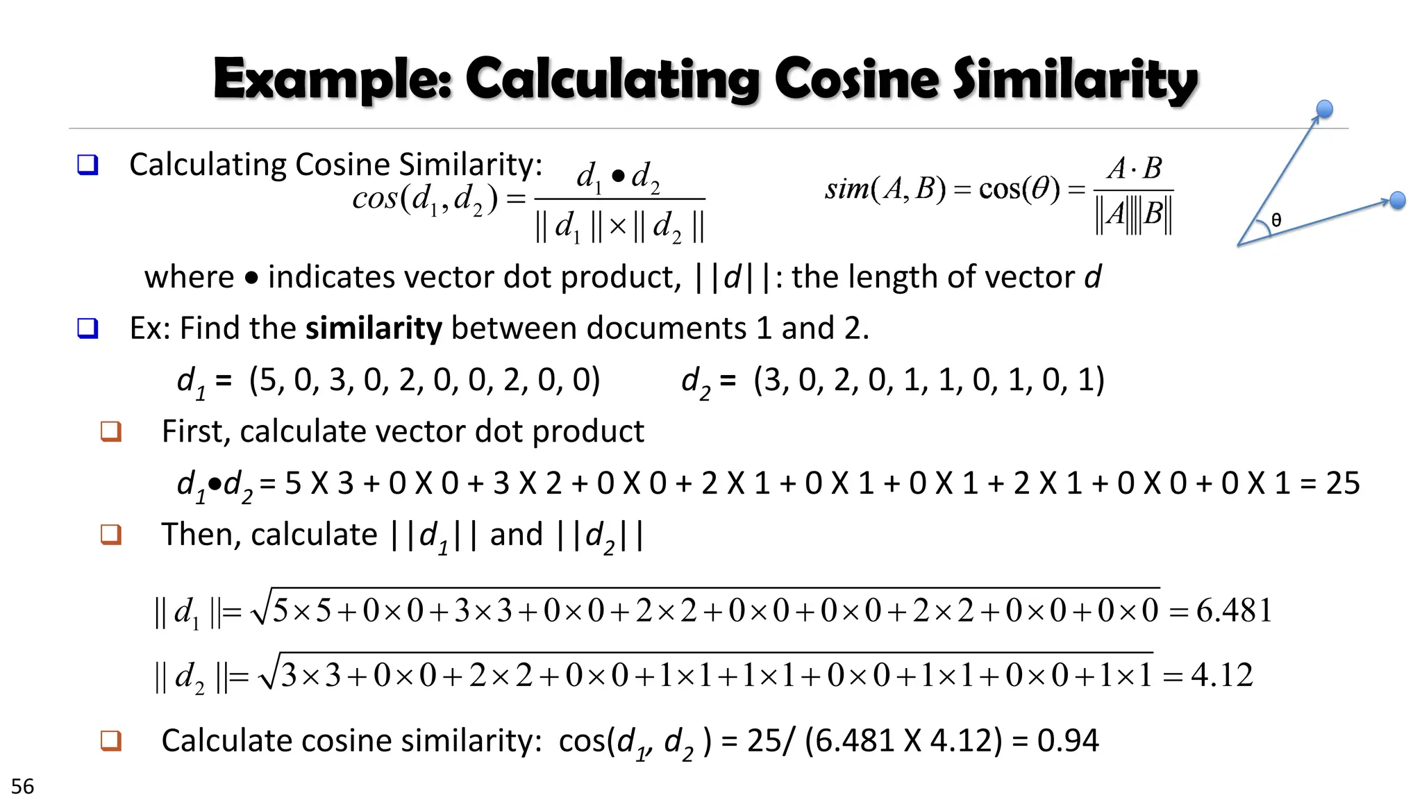
❑ Calculating Cosine Similarity:
where • indicates vector dot product, ||d||: the length of vector d
❑ Ex: Find the similarity between documents 1 and 2.
d1 = (5, 0, 3, 0, 2, 0, 0, 2, 0, 0) d2 = (3, 0, 2, 0, 1, 1, 0, 1, 0, 1)
❑ First, calculate vector dot product
d1•d2 = 5 X 3 + 0 X 0 + 3 X 2 + 0 X 0 + 2 X 1 + 0 X 1 + 0 X 1 + 2 X 1 + 0 X 0 + 0 X 1 = 25
❑ Then, calculate ||d1|| and ||d2||
❑ Calculate cosine similarity: cos(d1, d2 ) = 25/ (6.481 X 4.12) = 0.94
1 3 3 0 0 2 2 0 0 0 0 2 2 0 0 0 0 6.48
|| || 5 0 0 1
5
d + + +
=  +  +   + + + + =
     
2 3 2 2 0 0 1 1 1 1
|| | 0 0 1 1 0 0 1 1 4.12
| 3 0 0
d + + + + + + +
=  +  +         =
1 2
1 2
1 2
( , )
|| || || ||
d d
cos d d
d d
•
=


57
Capturing Hidden Semantics in Similarity
Measures
❑ The above similarity measures cannot capture hidden semantics
❑ Which pairs are more similar: Geometry, algebra, music, politics?
❑ The same bags of words may express rather different meanings
❑ “The cat bites a mouse” vs. “The mouse bites a cat”
❑ This is beyond what a vector space model can handle
❑ Moreover, objects can be composed of rather complex structures and
connections (e.g., graphs and networks)
❑ New similarity measures needed to handle complex semantics
❑ Ex. Distributive representation and representation learning

58
Data Quality, Data Cleaning and Data
Integration
❑ Data Quality Measures
❑ Data Cleaning
❑ Data Integration

59
What is Data Preprocessing? — Major Tasks
❑ Data cleaning
❑ Handle missing data, smooth noisy data, identify or remove outliers, and
resolve inconsistencies
❑ Data integration
❑ Integration of multiple databases, data cubes, or files
❑ Data reduction
❑ Dimensionality reduction
❑ Numerosity reduction
❑ Data compression
❑ Data transformation and data discretization
❑ Normalization
❑ Concept hierarchy generation

60
Why Preprocess the Data? — Data Quality Issues
❑ Measures for data quality: A multidimensional view
❑ Accuracy: correct or wrong, accurate or not
❑ Completeness: not recorded, unavailable, …
❑ Consistency: some modified but some not, dangling, …
❑ Timeliness: timely update?
❑ Believability: how trustable the data are correct?
❑ Interpretability: how easily the data can be understood?

61
Data Cleaning
❑ Data in the Real World Is Dirty: Lots of potentially incorrect data, e.g., instrument faulty,
human or computer error, and transmission error
❑ Incomplete: lacking attribute values, lacking certain attributes of interest, or containing
only aggregate data
❑ e.g., Occupation = “ ” (missing data)
❑ Noisy: containing noise, errors, or outliers
❑ e.g., Salary = “−10” (an error)
❑ Inconsistent: containing discrepancies in codes or names, e.g.,
❑ Age = “42”, Birthday = “03/07/2010”
❑ Was rating “1, 2, 3”, now rating “A, B, C”
❑ discrepancy between duplicate records
❑ Intentional (e.g., disguised missing data)
❑ Jan. 1 as everyone’s birthday?

62
Incomplete (Missing) Data
❑ Data is not always available
❑ E.g., many tuples have no recorded value for several attributes, such as
customer income in sales data
❑ Missing data may be due to
❑ Equipment malfunction
❑ Inconsistent with other recorded data and thus deleted
❑ Data were not entered due to misunderstanding
❑ Certain data may not be considered important at the time of entry
❑ Did not register history or changes of the data
❑ Missing data may need to be inferred

63
How to Handle Missing Data?
❑ Ignore the tuple: usually done when class label is missing (when doing
classification)—not effective when the % of missing values per attribute varies
considerably
❑ Fill in the missing value manually: tedious + infeasible?
❑ Fill in it automatically with
❑ a global constant : e.g., “unknown”, a new class?!
❑ the attribute mean
❑ the attribute mean for all samples belonging to the same class: smarter
❑ the most probable value: inference-based such as Bayesian formula or decision
tree

64
Noisy Data
❑ Noise: random error or variance in a measured variable
❑ Incorrect attribute values may be due to
❑ Faulty data collection instruments
❑ Data entry problems
❑ Data transmission problems
❑ Technology limitation
❑ Inconsistency in naming convention
❑ Other data problems
❑ Duplicate records
❑ Incomplete data
❑ Inconsistent data

65
How to Handle Noisy Data?
❑ Binning
❑ First sort data and partition into (equal-frequency) bins
❑ Then one can smooth by bin means, smooth by bin median, smooth by bin
boundaries, etc.
❑ Regression
❑ Smooth by fitting the data into regression functions
❑ Clustering
❑ Detect and remove outliers
❑ Semi-supervised: Combined computer and human inspection
❑ Detect suspicious values and check by human (e.g., deal with possible outliers)

66
Data Cleaning as a Process
❑ Data discrepancy detection
❑ Use metadata (e.g., domain, range, dependency, distribution)
❑ Check field overloading
❑ Check uniqueness rule, consecutive rule and null rule
❑ Use commercial tools
❑ Data scrubbing: use simple domain knowledge (e.g., postal code, spell-check) to
detect errors and make corrections
❑ Data auditing: by analyzing data to discover rules and relationship to detect violators
(e.g., correlation and clustering to find outliers)
❑ Data migration and integration
❑ Data migration tools: allow transformations to be specified
❑ ETL (Extraction/Transformation/Loading) tools: allow users to specify transformations
through a graphical user interface
❑ Integration of the two processes
❑ Iterative and interactive (e.g., Potter’s Wheels)

67
Data Integration
❑ Data integration
❑ Combining data from multiple sources into a coherent store
❑ Why data integration?
❑ Help reduce/avoid noise
❑ Get a more complete picture
❑ Improve mining speed and quality
❑ Schema integration:
❑ e.g., A.cust-id  B.cust-#
❑ Integrate metadata from different sources
❑ Entity identification:
❑ Identify real world entities from multiple data sources, e.g., Bill Clinton =
William Clinton

68
Handling Noise in Data Integration
❑ Detecting data value conflicts
❑ For the same real world entity, attribute values from different sources are
different
❑ Possible reasons: no reason, different representations, different scales, e.g.,
metric vs. British units
❑ Resolving conflict information
❑ Take the mean/median/mode/max/min
❑ Take the most recent
❑ Truth finding: consider the source quality
❑ Data cleaning + data integration

69
Handling Redundancy in Data Integration
❑ Redundant data occur often when integration of multiple databases
❑ Object identification: The same attribute or object may have different names in
different databases
❑ Derivable data: One attribute may be a “derived” attribute in another table,
e.g., annual revenue
❑ What’s the problem?
❑ 𝑌 = 2𝑋 → 𝑌 = 𝑋1 + 𝑋2 𝑌 = 3𝑋1 − 𝑋2 𝑌 = −1291𝑋1 + 1293𝑋2
❑ Redundant attributes may be detected by correlation analysis and covariance
analysis

70
Data Transformation
❑ Normalization
❑ Discretization
❑ Data Compression
❑ Sampling

71
Data Transformation
❑ A function that maps the entire set of values of a given attribute to a new set of
replacement values s.t. each old value can be identified with one of the new values
❑ Methods
❑ Smoothing: Remove noise from data
❑ Attribute/feature construction
❑ New attributes constructed from the given ones
❑ Aggregation: Summarization, data cube construction
❑ Normalization: Scaled to fall within a smaller, specified range
❑ min-max normalization
❑ z-score normalization
❑ normalization by decimal scaling
❑ Discretization: Concept hierarchy climbing

72
Normalization
❑ Min-max normalization: to [new_minA, new_maxA]
❑ Ex. Let income range $12,000 to $98,000 normalized to [0.0, 1.0]
❑ Then $73,000 is mapped to
❑ Z-score normalization (μ: mean, σ: standard deviation):
❑ Ex. Let μ = 54,000, σ = 16,000. Then
❑ Normalization by decimal scaling
716
.
0
0
)
0
0
.
1
(
000
,
12
000
,
98
000
,
12
600
,
73
=
+
−
−
−
A
A
A
A
A
A
min
new
min
new
max
new
min
max
min
v
v _
)
_
_
(
' +
−
−
−
=
A
A
v
v


−
=
'
j
v
v
10
'= Where j is the smallest integer such that Max(|ν’|) < 1
225
.
1
000
,
16
000
,
54
600
,
73
=
−
Z-score: The distance between the raw score and the
population mean in the unit of the standard deviation

73
Discretization
❑ Three types of attributes
❑ Nominal—values from an unordered set, e.g., color, profession
❑ Ordinal—values from an ordered set, e.g., military or academic rank
❑ Numeric—real numbers, e.g., integer or real numbers
❑ Discretization: Divide the range of a continuous attribute into intervals
❑ Interval labels can then be used to replace actual data values
❑ Reduce data size by discretization
❑ Supervised vs. unsupervised
❑ Split (top-down) vs. merge (bottom-up)
❑ Discretization can be performed recursively on an attribute
❑ Prepare for further analysis, e.g., classification

74
Data Discretization Methods
❑ Binning
❑ Top-down split, unsupervised
❑ Histogram analysis
❑ Top-down split, unsupervised
❑ Clustering analysis
❑ Unsupervised, top-down split or bottom-up merge
❑ Decision-tree analysis
❑ Supervised, top-down split
❑ Correlation (e.g., 2) analysis
❑ Unsupervised, bottom-up merge
❑ Note: All the methods can be applied recursively

75
Simple Discretization: Binning
❑ Equal-width (distance) partitioning
❑ Divides the range into N intervals of equal size: uniform grid
❑ if A and B are the lowest and highest values of the attribute, the width of
intervals will be: W = (B –A)/N.
❑ The most straightforward, but outliers may dominate presentation
❑ Skewed data is not handled well
❑ Equal-depth (frequency) partitioning
❑ Divides the range into N intervals, each containing approximately same number
of samples
❑ Good data scaling
❑ Managing categorical attributes can be tricky

76
Example: Binning Methods for Data Smoothing
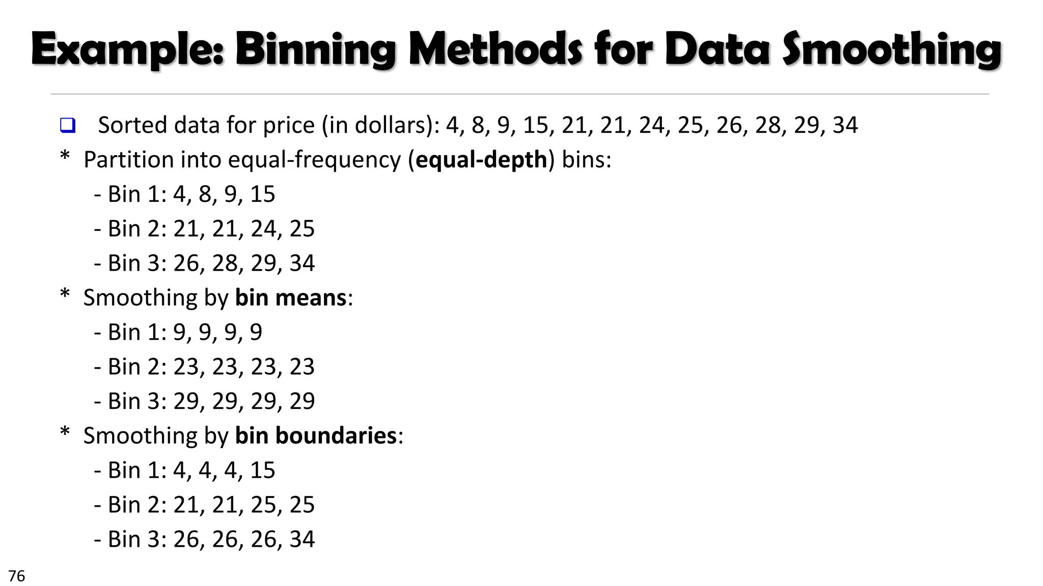
❑ Sorted data for price (in dollars): 4, 8, 9, 15, 21, 21, 24, 25, 26, 28, 29, 34
* Partition into equal-frequency (equal-depth) bins:
- Bin 1: 4, 8, 9, 15
- Bin 2: 21, 21, 24, 25
- Bin 3: 26, 28, 29, 34
* Smoothing by bin means:
- Bin 1: 9, 9, 9, 9
- Bin 2: 23, 23, 23, 23
- Bin 3: 29, 29, 29, 29
* Smoothing by bin boundaries:
- Bin 1: 4, 4, 4, 15
- Bin 2: 21, 21, 25, 25
- Bin 3: 26, 26, 26, 34

77
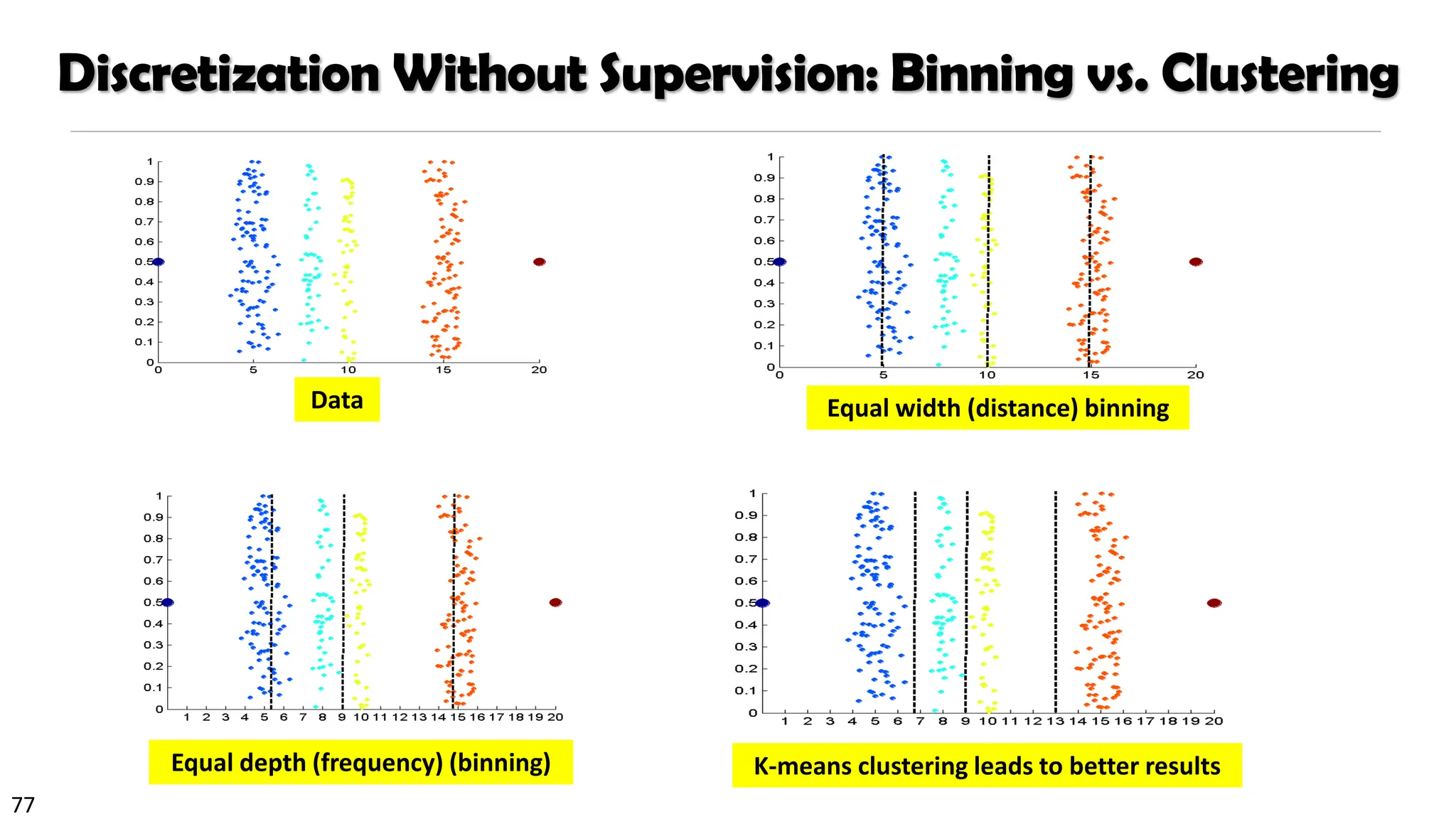
Discretization Without Supervision: Binning vs. Clustering
Data
Equal depth (frequency) (binning) K-means clustering leads to better results
Equal width (distance) binning

78
Discretization by Classification & Correlation Analysis
❑ Classification (e.g., decision tree analysis)
❑ Supervised: Given class labels, e.g., cancerous vs. benign
❑ Using entropy to determine split point (discretization point)
❑ Top-down, recursive split
❑ Details to be covered in Chapter “Classification”
❑ Correlation analysis (e.g., Chi-merge: χ2-based discretization)
❑ Supervised: use class information
❑ Bottom-up merge: Find the best neighboring intervals (those having similar
distributions of classes, i.e., low χ2 values) to merge
❑ Merge performed recursively, until a predefined stopping condition

79
Concept Hierarchy Generation
❑ Concept hierarchy organizes concepts (i.e., attribute values) hierarchically and is
usually associated with each dimension in a data warehouse
❑ Concept hierarchies facilitate drilling and rolling in data warehouses to view data
in multiple granularity
❑ Concept hierarchy formation: Recursively reduce the data by collecting and
replacing low level concepts (such as numeric values for age) by higher level
concepts (such as youth, adult, or senior)
❑ Concept hierarchies can be explicitly specified by domain experts and/or data
warehouse designers
❑ Concept hierarchy can be automatically formed for both numeric and nominal
data—For numeric data, use discretization methods shown

80
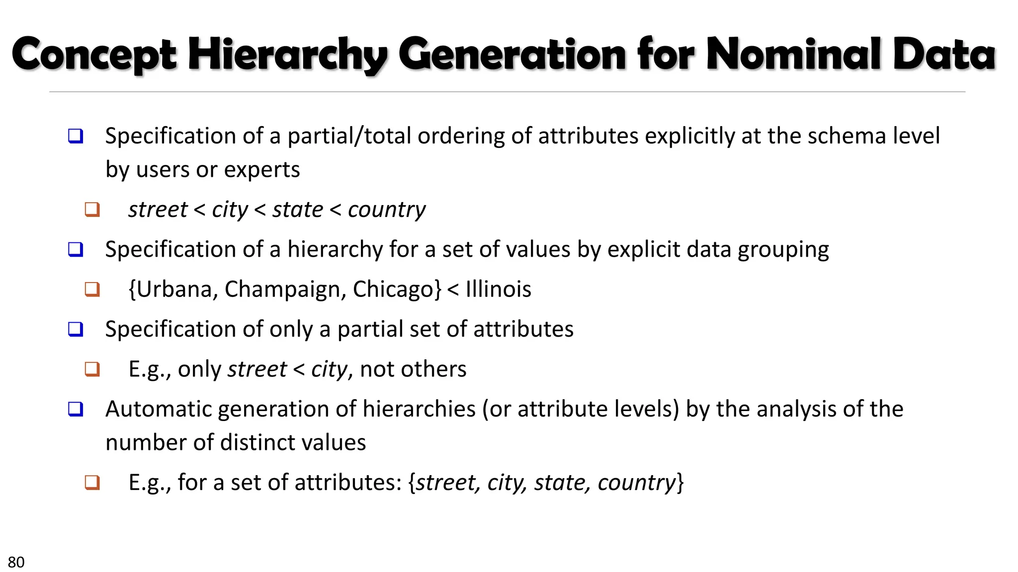
Concept Hierarchy Generation for Nominal Data
❑ Specification of a partial/total ordering of attributes explicitly at the schema level
by users or experts
❑ street < city < state < country
❑ Specification of a hierarchy for a set of values by explicit data grouping
❑ {Urbana, Champaign, Chicago} < Illinois
❑ Specification of only a partial set of attributes
❑ E.g., only street < city, not others
❑ Automatic generation of hierarchies (or attribute levels) by the analysis of the
number of distinct values
❑ E.g., for a set of attributes: {street, city, state, country}

81
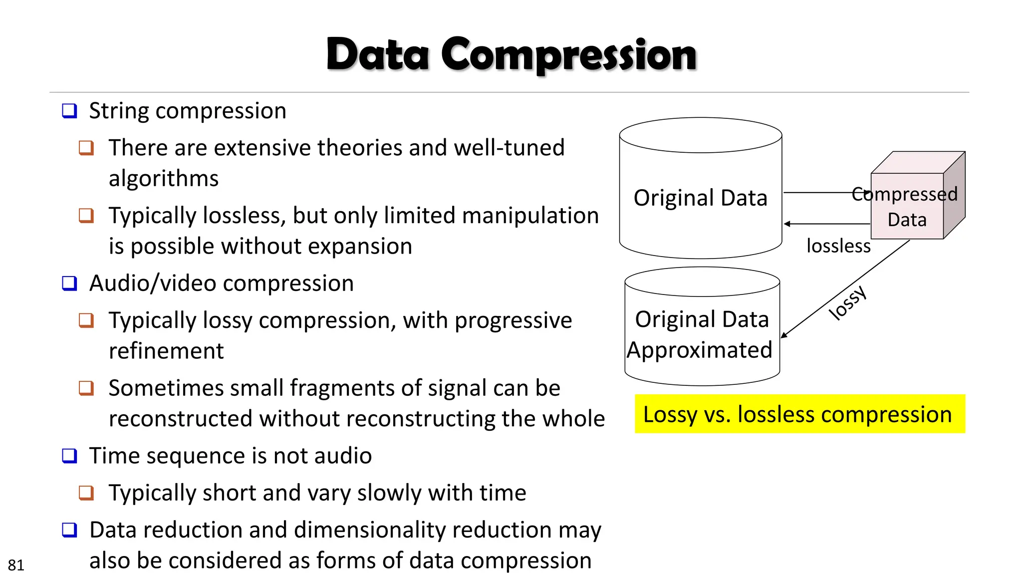
Data Compression
❑ String compression
❑ There are extensive theories and well-tuned
algorithms
❑ Typically lossless, but only limited manipulation
is possible without expansion
❑ Audio/video compression
❑ Typically lossy compression, with progressive
refinement
❑ Sometimes small fragments of signal can be
reconstructed without reconstructing the whole
❑ Time sequence is not audio
❑ Typically short and vary slowly with time
❑ Data reduction and dimensionality reduction may
also be considered as forms of data compression
Original Data Compressed
Data
lossless
Original Data
Approximated
Lossy vs. lossless compression

82
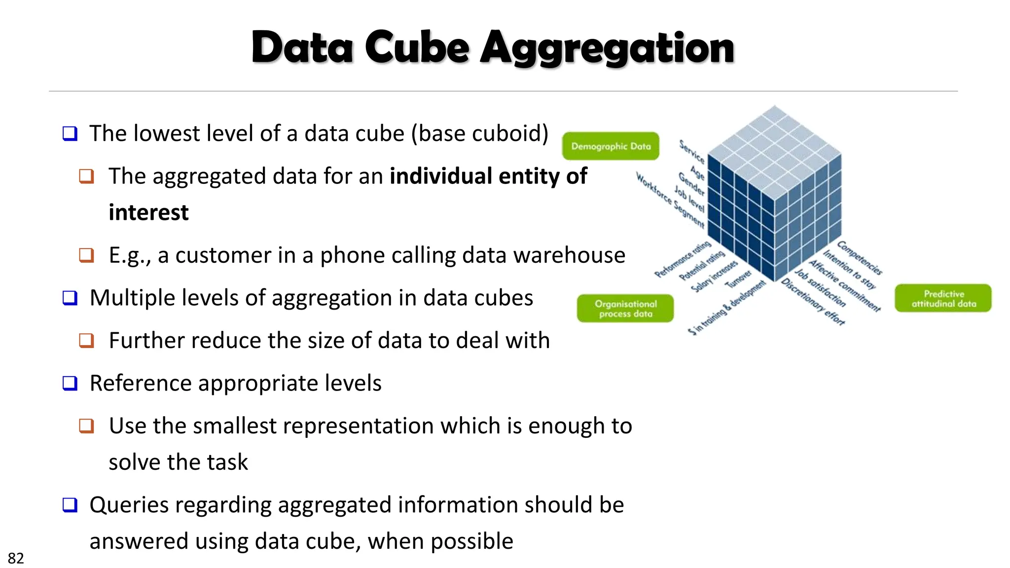
Data Cube Aggregation
❑ The lowest level of a data cube (base cuboid)
❑ The aggregated data for an individual entity of
interest
❑ E.g., a customer in a phone calling data warehouse
❑ Multiple levels of aggregation in data cubes
❑ Further reduce the size of data to deal with
❑ Reference appropriate levels
❑ Use the smallest representation which is enough to
solve the task
❑ Queries regarding aggregated information should be
answered using data cube, when possible

83
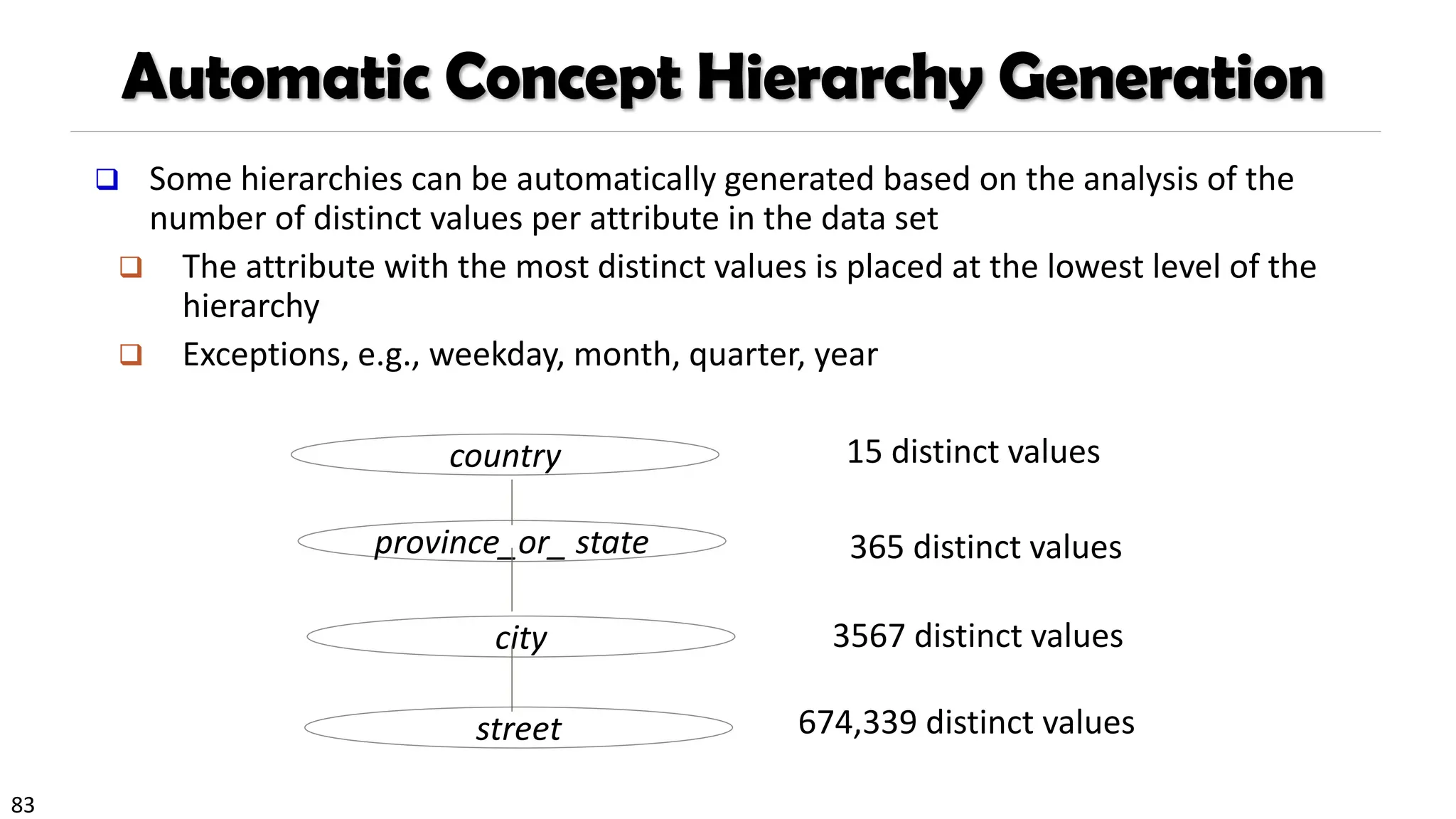
Automatic Concept Hierarchy Generation
❑ Some hierarchies can be automatically generated based on the analysis of the
number of distinct values per attribute in the data set
❑ The attribute with the most distinct values is placed at the lowest level of the
hierarchy
❑ Exceptions, e.g., weekday, month, quarter, year
country
province_or_ state
city
street
15 distinct values
365 distinct values
3567 distinct values
674,339 distinct values

84
Sampling
❑ Sampling: obtaining a small sample s to represent the whole data set N
❑ Allow a mining algorithm to run in complexity that is potentially sub-linear to the
size of the data
❑ Key principle: Choose a representative subset of the data
❑ Simple random sampling may have very poor performance in the presence of
skew
❑ Develop adaptive sampling methods, e.g., stratified sampling:
❑ Note: Sampling may not reduce database I/Os (page at a time)

85
Raw Data
Types of Sampling
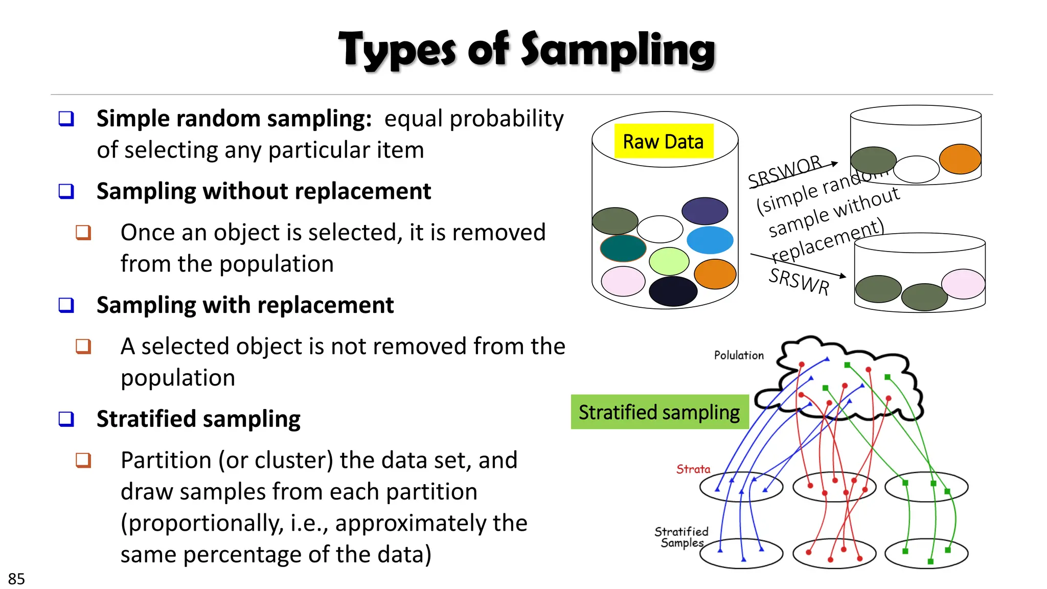
❑ Simple random sampling: equal probability
of selecting any particular item
❑ Sampling without replacement
❑ Once an object is selected, it is removed
from the population
❑ Sampling with replacement
❑ A selected object is not removed from the
population
❑ Stratified sampling
❑ Partition (or cluster) the data set, and
draw samples from each partition
(proportionally, i.e., approximately the
same percentage of the data)
Stratified sampling

86
Data Reduction
❑ Data reduction:
❑ Obtain a reduced representation of the data set
❑ much smaller in volume but yet produces almost the same analytical results
❑ Why data reduction?—A database/data warehouse may store terabytes of data
❑ Complex analysis may take a very long time to run on the complete data set
❑ Methods for data reduction (also data size reduction or numerosity reduction)
❑ Regression and Log-Linear Models
❑ Histograms, clustering, sampling
❑ Data cube aggregation
❑ Data compression

87
Data Reduction: Parametric vs. Non-Parametric Methods
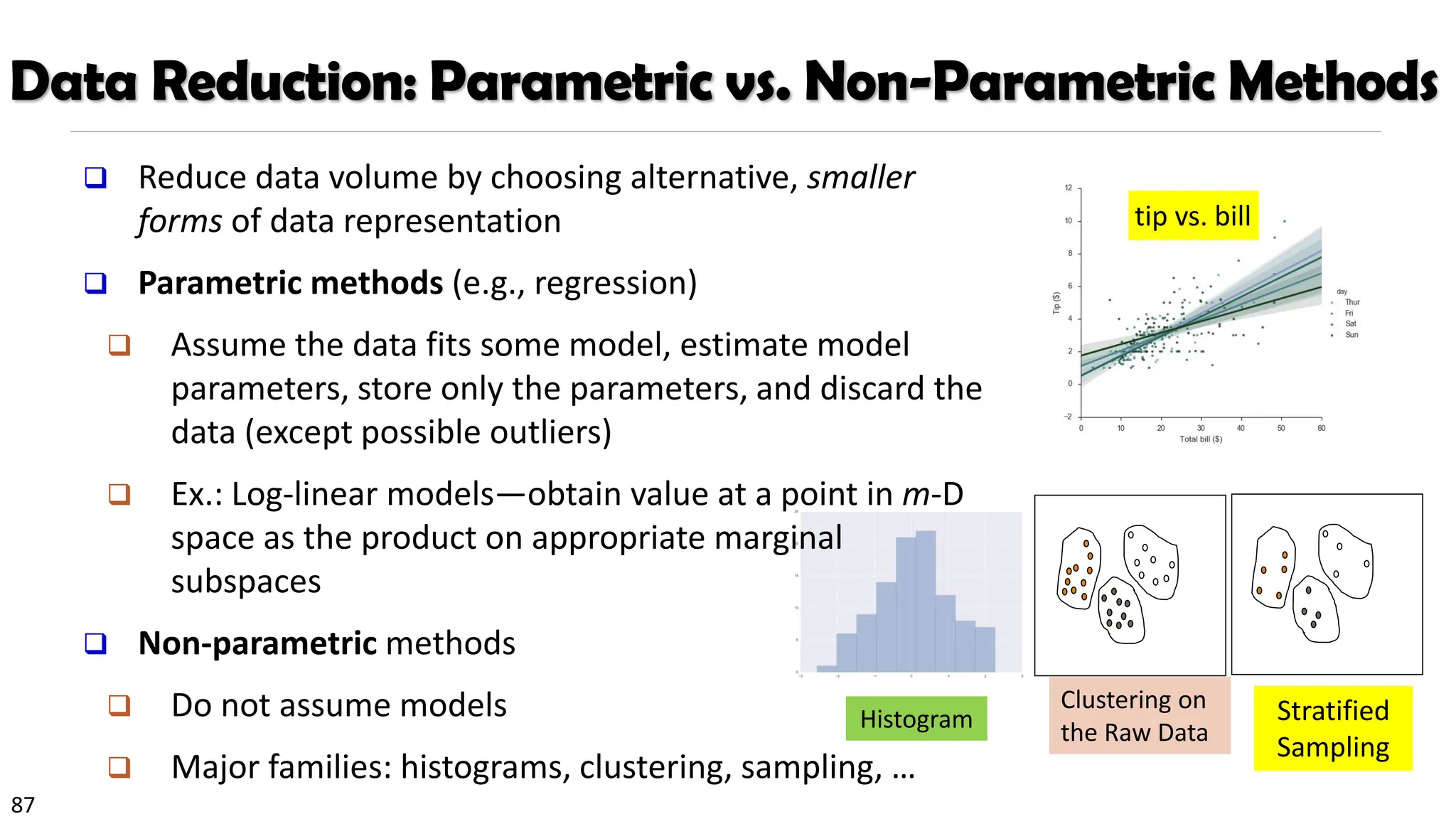
❑ Reduce data volume by choosing alternative, smaller
forms of data representation
❑ Parametric methods (e.g., regression)
❑ Assume the data fits some model, estimate model
parameters, store only the parameters, and discard the
data (except possible outliers)
❑ Ex.: Log-linear models—obtain value at a point in m-D
space as the product on appropriate marginal
subspaces
❑ Non-parametric methods
❑ Do not assume models
❑ Major families: histograms, clustering, sampling, …
tip vs. bill
Clustering on
the Raw Data
Stratified
Sampling
Histogram

88
Parametric Data Reduction: Regression Analysis
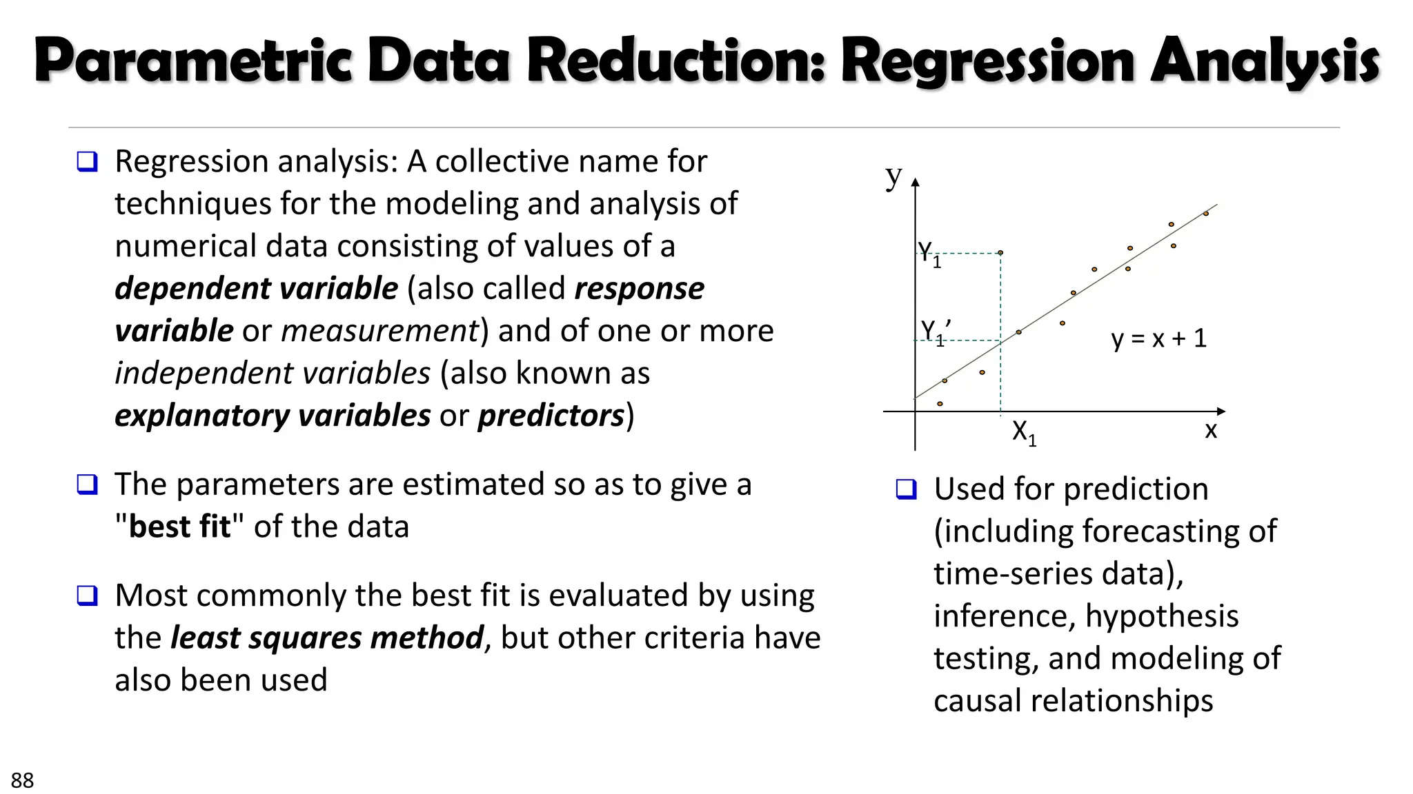
❑ Regression analysis: A collective name for
techniques for the modeling and analysis of
numerical data consisting of values of a
dependent variable (also called response
variable or measurement) and of one or more
independent variables (also known as
explanatory variables or predictors)
❑ The parameters are estimated so as to give a
"best fit" of the data
❑ Most commonly the best fit is evaluated by using
the least squares method, but other criteria have
also been used
❑ Used for prediction
(including forecasting of
time-series data),
inference, hypothesis
testing, and modeling of
causal relationships
y
x
y = x + 1
X1
Y1
Y1’

89
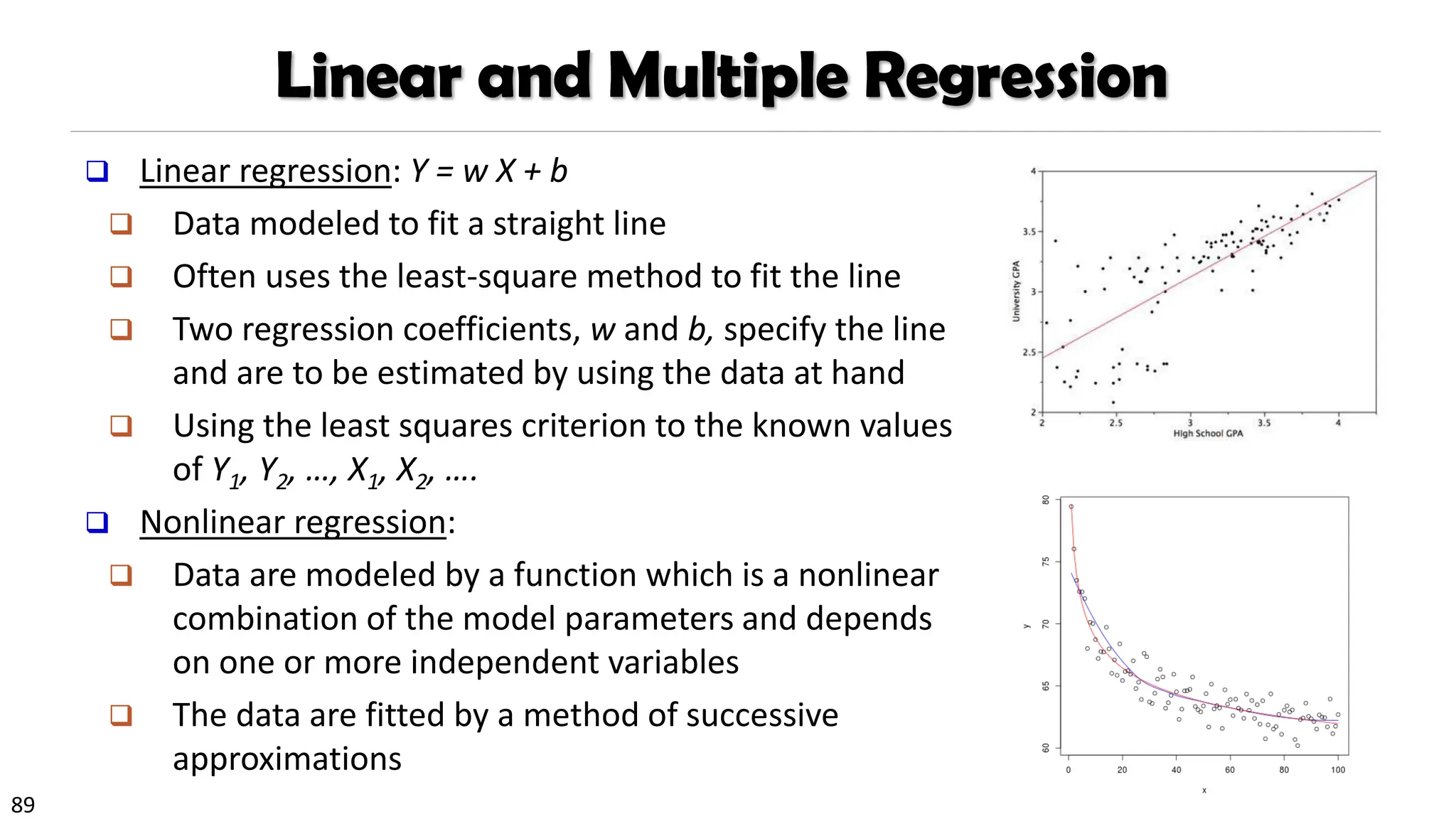
❑ Linear regression: Y = w X + b
❑ Data modeled to fit a straight line
❑ Often uses the least-square method to fit the line
❑ Two regression coefficients, w and b, specify the line
and are to be estimated by using the data at hand
❑ Using the least squares criterion to the known values
of Y1, Y2, …, X1, X2, ….
❑ Nonlinear regression:
❑ Data are modeled by a function which is a nonlinear
combination of the model parameters and depends
on one or more independent variables
❑ The data are fitted by a method of successive
approximations
Linear and Multiple Regression

90
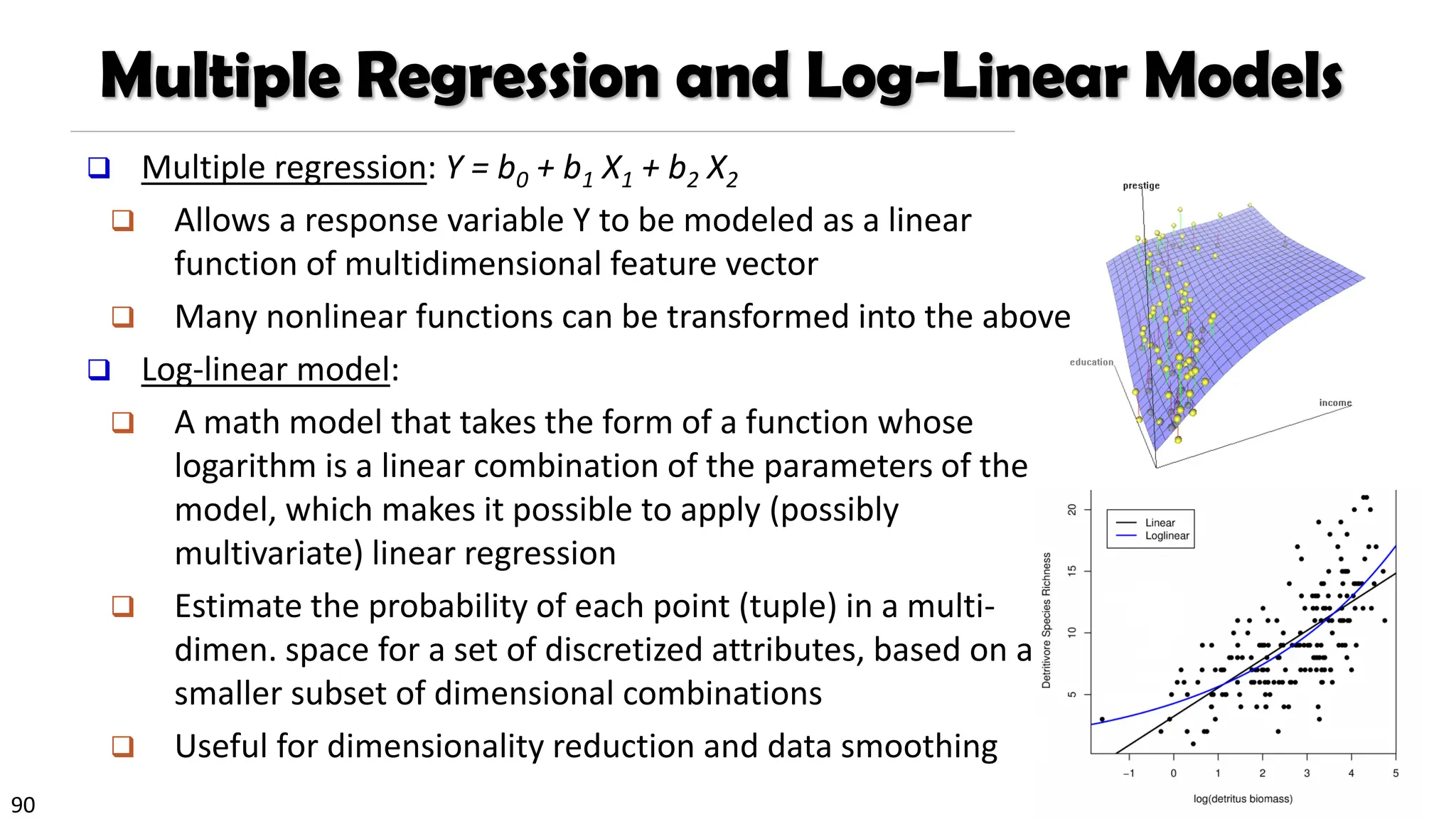
❑ Multiple regression: Y = b0 + b1 X1 + b2 X2
❑ Allows a response variable Y to be modeled as a linear
function of multidimensional feature vector
❑ Many nonlinear functions can be transformed into the above
❑ Log-linear model:
❑ A math model that takes the form of a function whose
logarithm is a linear combination of the parameters of the
model, which makes it possible to apply (possibly
multivariate) linear regression
❑ Estimate the probability of each point (tuple) in a multi-
dimen. space for a set of discretized attributes, based on a
smaller subset of dimensional combinations
❑ Useful for dimensionality reduction and data smoothing
Multiple Regression and Log-Linear Models

91
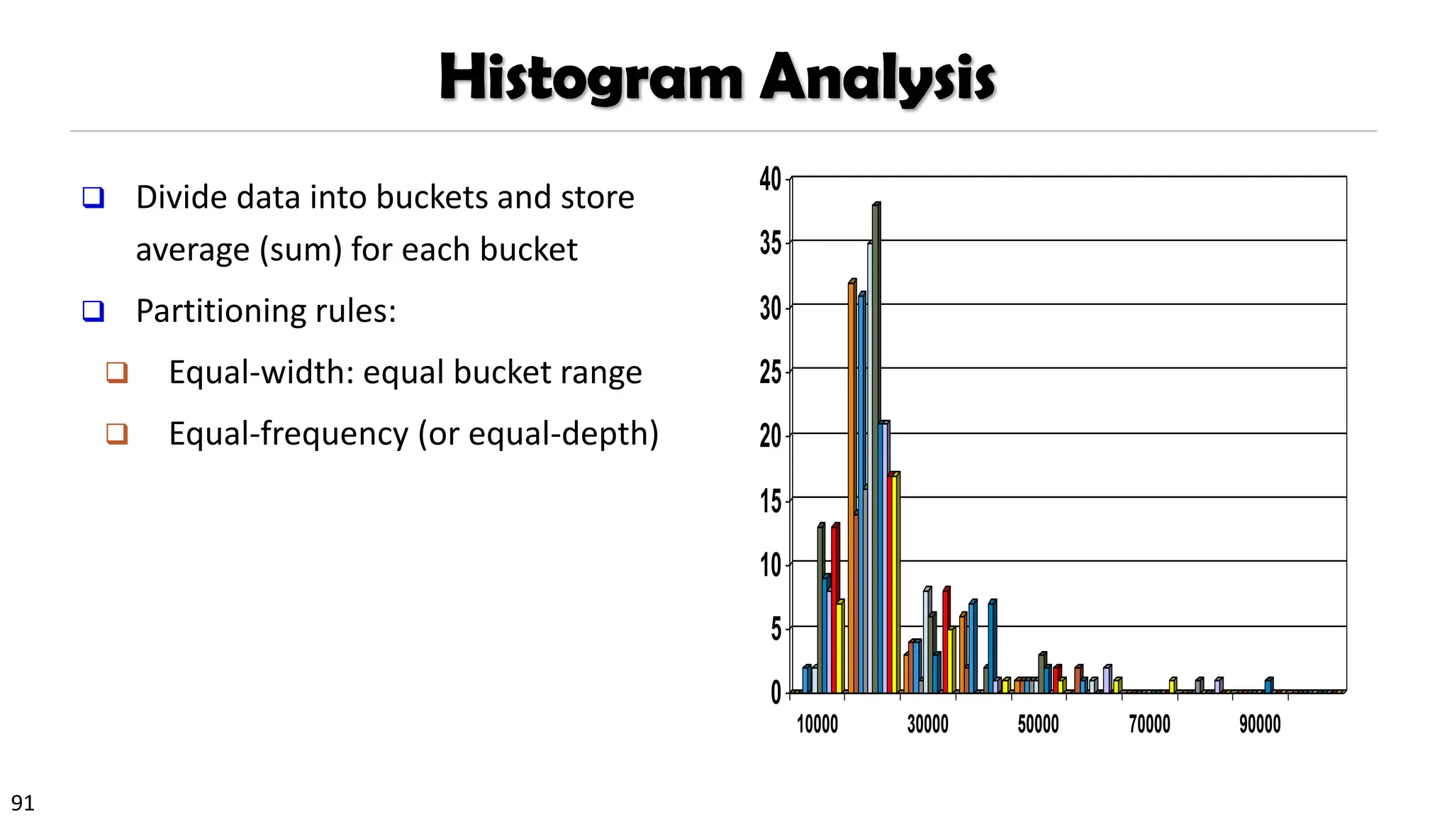
Histogram Analysis
❑ Divide data into buckets and store
average (sum) for each bucket
❑ Partitioning rules:
❑ Equal-width: equal bucket range
❑ Equal-frequency (or equal-depth)
0
5
10
15
20
25
30
35
40
10000 30000 50000 70000 90000

92
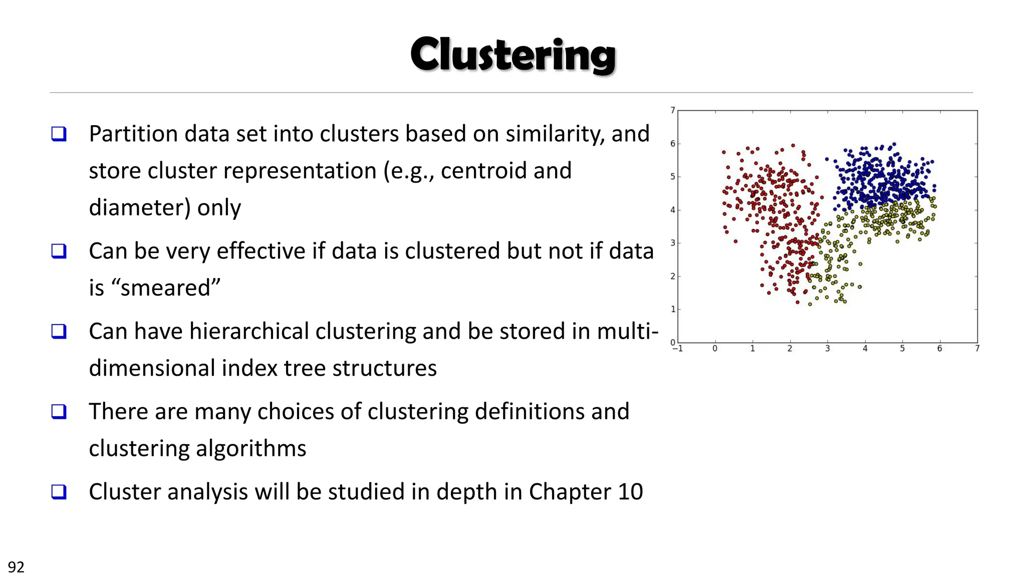
Clustering
❑ Partition data set into clusters based on similarity, and
store cluster representation (e.g., centroid and
diameter) only
❑ Can be very effective if data is clustered but not if data
is “smeared”
❑ Can have hierarchical clustering and be stored in multi-
dimensional index tree structures
❑ There are many choices of clustering definitions and
clustering algorithms
❑ Cluster analysis will be studied in depth in Chapter 10

93
Dimensionality Reduction
❑ What Is Dimensionality Reduction?
❑ Dimensionality Reduction Methods
❑ Principal Component Analysis
❑ Attribute Subset Selection
❑ Nonlinear Dimensionality Reduction Methods

94
What Is Dimensionality Reduction?
❑ Curse of dimensionality
❑ When dimensionality increases, data becomes increasingly sparse
❑ Density and distance between points, which is critical to clustering, outlier
analysis, becomes less meaningful
❑ The possible combinations of subspaces will grow exponentially
❑ Dimensionality reduction
❑ Reducing the number of random variables under consideration, via obtaining a set
of principal variables
❑ Advantages of dimensionality reduction
❑ Avoid the curse of dimensionality
❑ Help eliminate irrelevant features and reduce noise
❑ Reduce time and space required in data mining
❑ Allow easier visualization

95
Dimensionality Reduction Methods
❑ Dimensionality reduction methodologies
❑ Feature selection: Find a subset of the original variables (or features, attributes)
❑ Feature extraction: Transform the data in the high-dimensional space to a space
of fewer dimensions
❑ Some typical dimensionality reduction methods
❑ Principal Component Analysis
❑ Attribute Subset Selection
❑ Nonlinear Dimensionality Reduction

96
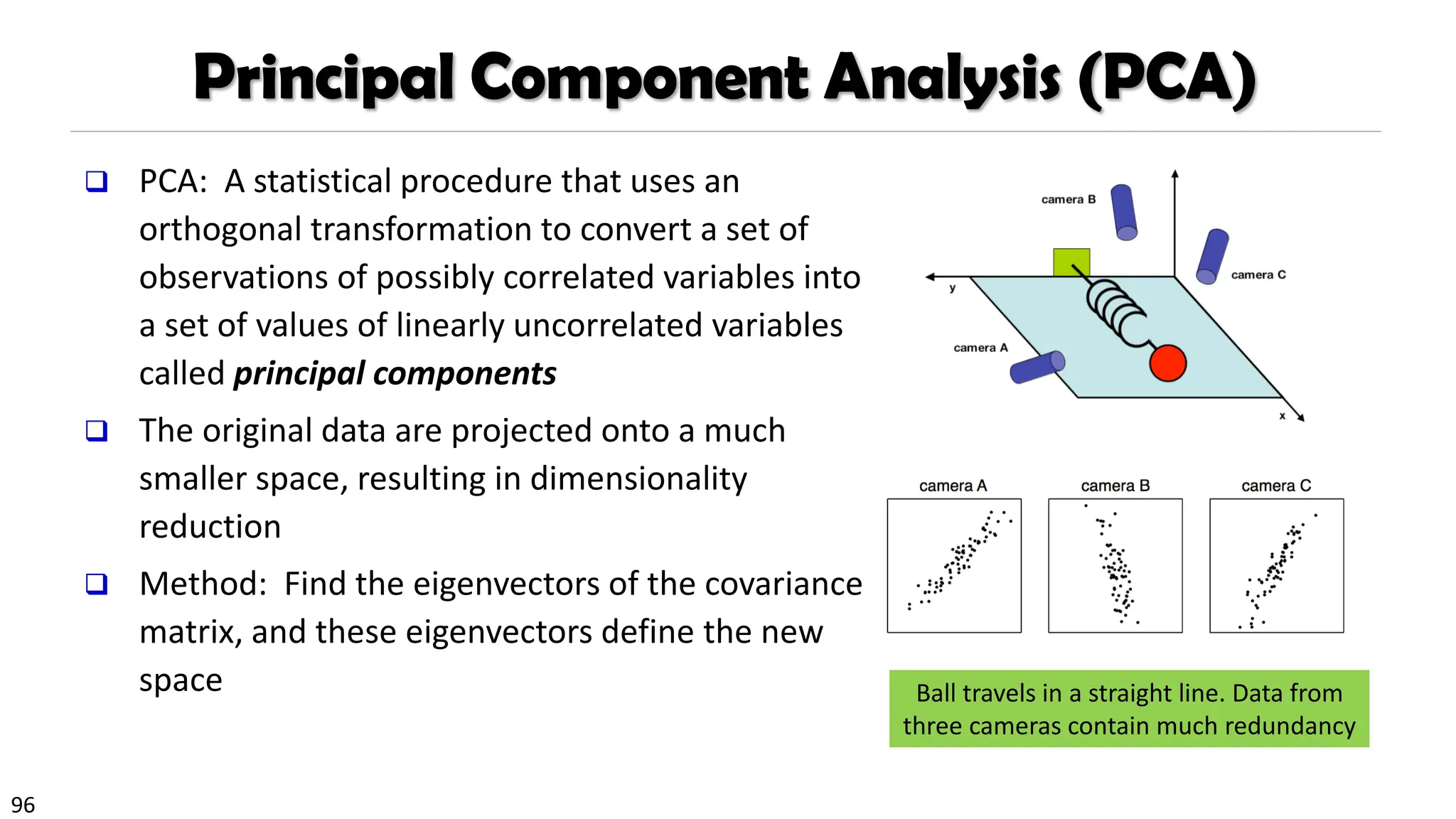
Principal Component Analysis (PCA)
❑ PCA: A statistical procedure that uses an
orthogonal transformation to convert a set of
observations of possibly correlated variables into
a set of values of linearly uncorrelated variables
called principal components
❑ The original data are projected onto a much
smaller space, resulting in dimensionality
reduction
❑ Method: Find the eigenvectors of the covariance
matrix, and these eigenvectors define the new
space Ball travels in a straight line. Data from
three cameras contain much redundancy

97
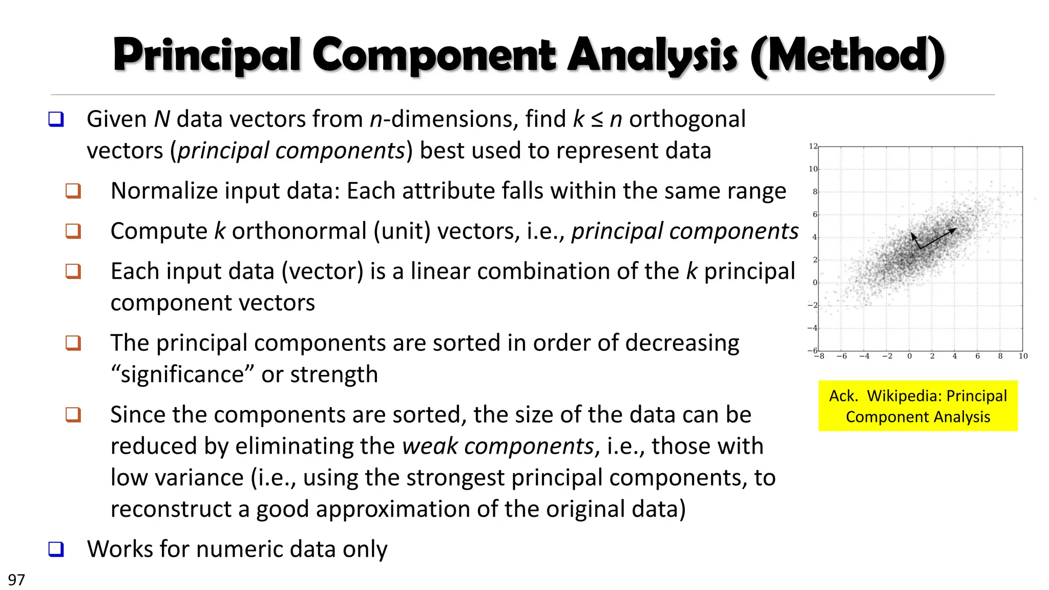
❑ Given N data vectors from n-dimensions, find k ≤ n orthogonal
vectors (principal components) best used to represent data
❑ Normalize input data: Each attribute falls within the same range
❑ Compute k orthonormal (unit) vectors, i.e., principal components
❑ Each input data (vector) is a linear combination of the k principal
component vectors
❑ The principal components are sorted in order of decreasing
“significance” or strength
❑ Since the components are sorted, the size of the data can be
reduced by eliminating the weak components, i.e., those with
low variance (i.e., using the strongest principal components, to
reconstruct a good approximation of the original data)
❑ Works for numeric data only
Principal Component Analysis (Method)
Ack. Wikipedia: Principal
Component Analysis

98
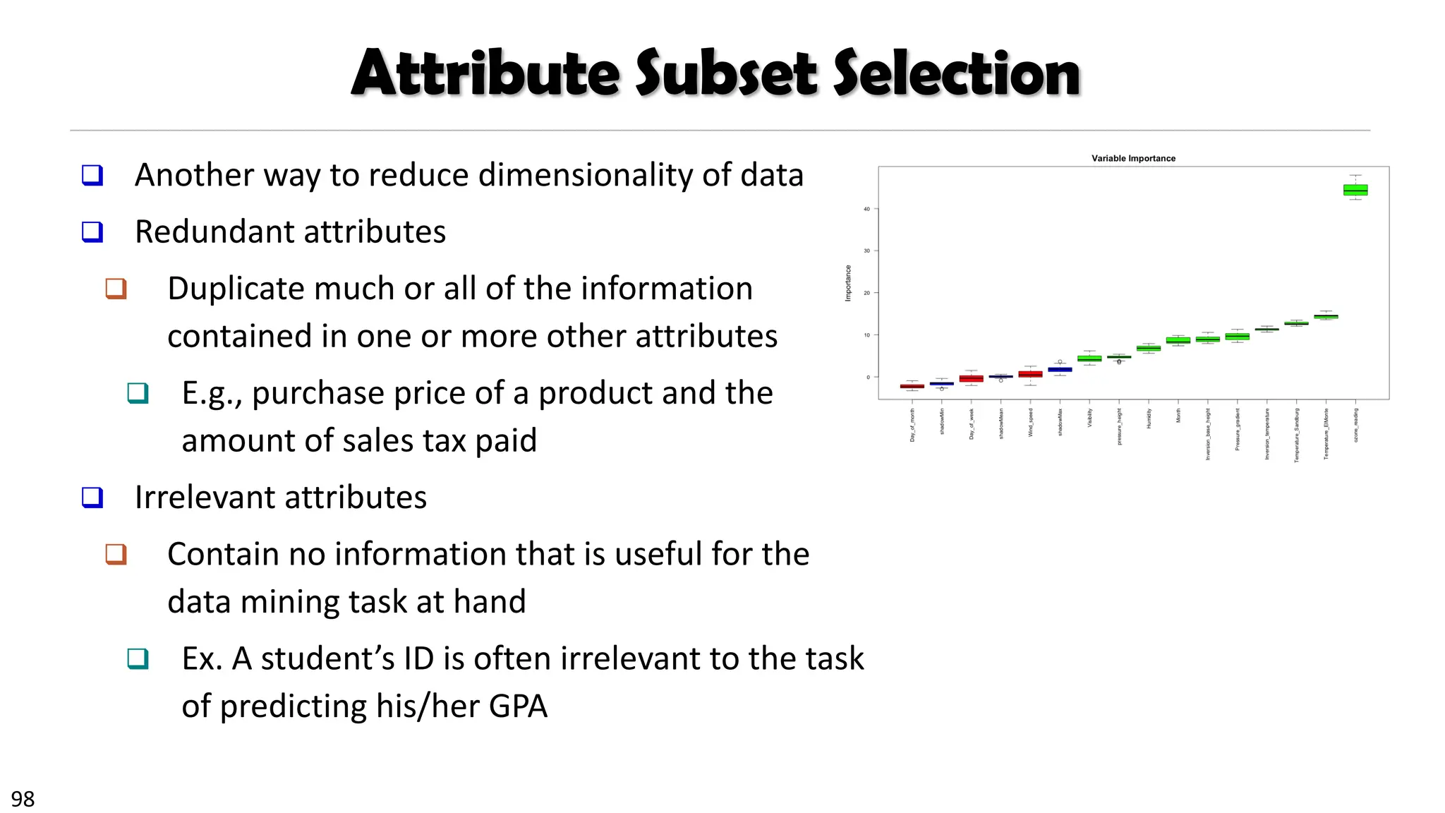
Attribute Subset Selection
❑ Another way to reduce dimensionality of data
❑ Redundant attributes
❑ Duplicate much or all of the information
contained in one or more other attributes
❑ E.g., purchase price of a product and the
amount of sales tax paid
❑ Irrelevant attributes
❑ Contain no information that is useful for the
data mining task at hand
❑ Ex. A student’s ID is often irrelevant to the task
of predicting his/her GPA

99
Heuristic Search in Attribute Selection
❑ There are 2d possible attribute combinations of d attributes
❑ Typical heuristic attribute selection methods:
❑ Best single attribute under the attribute independence assumption: choose by
significance tests
❑ Best step-wise feature selection:
❑ The best single-attribute is picked first
❑ Then next best attribute condition to the first, ...
❑ Step-wise attribute elimination:
❑ Repeatedly eliminate the worst attribute
❑ Best combined attribute selection and elimination
❑ Optimal branch and bound:
❑ Use attribute elimination and backtracking

100
Attribute Creation (Feature Generation)
❑ Create new attributes (features) that can capture the important information in a
data set more effectively than the original ones
❑ Three general methodologies
❑ Attribute extraction
❑ Domain-specific
❑ Mapping data to new space (see data reduction)
❑ E.g., Fourier transformation, wavelet transformation, manifold approaches (not
covered)
❑ Attribute construction
❑ Combining features (see discriminative frequent patterns in Chapter on
“Advanced Classification”)
❑ Data discretization

101
Nonlinear Dimensionality Reduction Methods
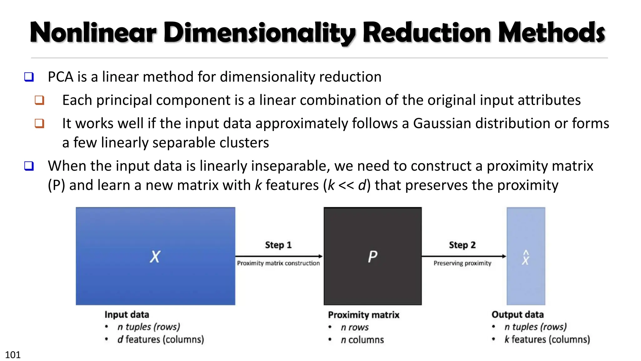
❑ PCA is a linear method for dimensionality reduction
❑ Each principal component is a linear combination of the original input attributes
❑ It works well if the input data approximately follows a Gaussian distribution or forms
a few linearly separable clusters
❑ When the input data is linearly inseparable, we need to construct a proximity matrix
(P) and learn a new matrix with k features (k << d) that preserves the proximity

102
Nonlinear Dimensionality Reduction (I): Kernel PCA (KPCA)
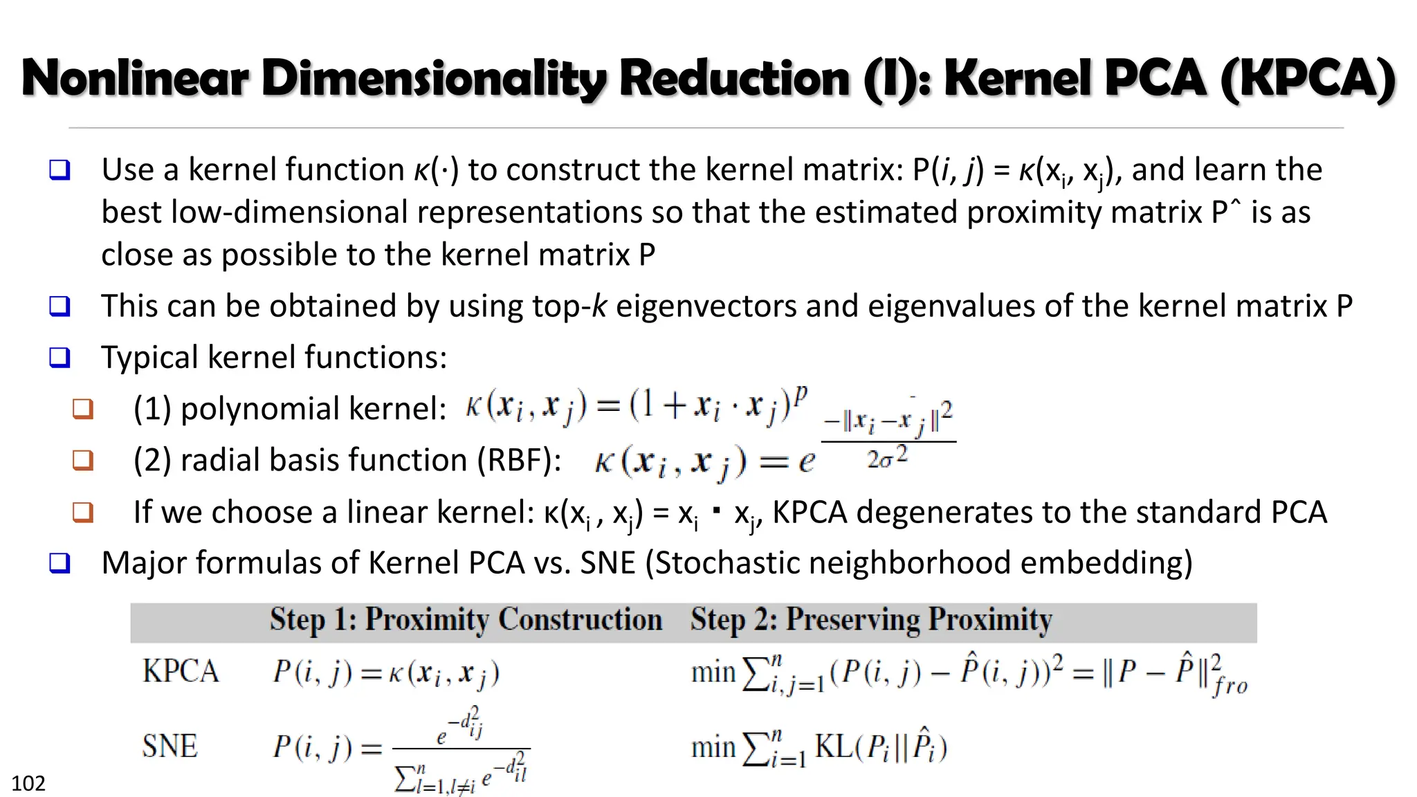
❑ Use a kernel function κ(·) to construct the kernel matrix: P(i, j) = κ(xi, xj), and learn the
best low-dimensional representations so that the estimated proximity matrix Pˆ is as
close as possible to the kernel matrix P
❑ This can be obtained by using top-k eigenvectors and eigenvalues of the kernel matrix P
❑ Typical kernel functions:
❑ (1) polynomial kernel:
❑ (2) radial basis function (RBF):
❑ If we choose a linear kernel: κ(xi , xj) = xi・xj, KPCA degenerates to the standard PCA
❑ Major formulas of Kernel PCA vs. SNE (Stochastic neighborhood embedding)

103
Nonlinear Dimensionality Reduction (II): SNE
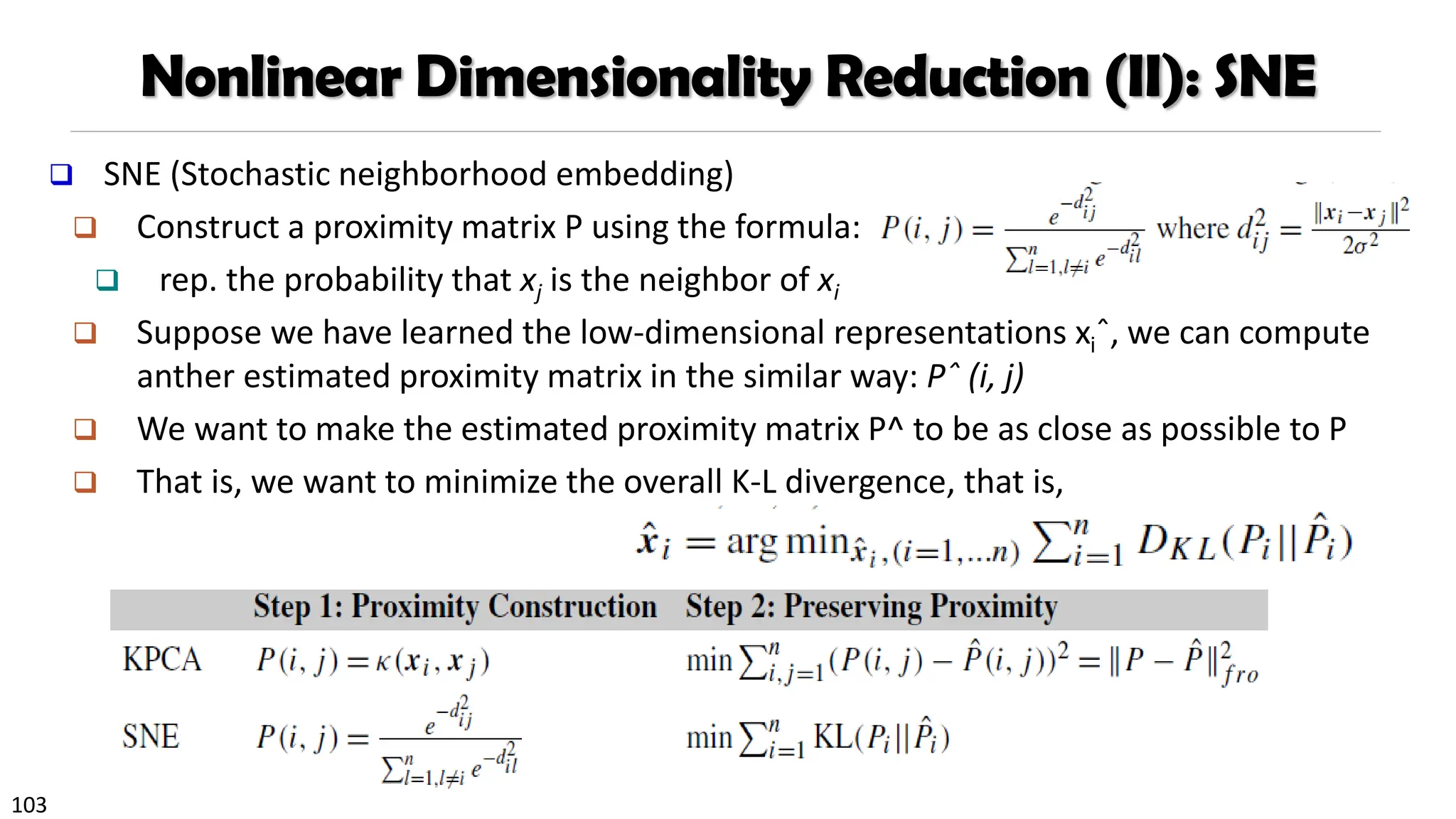
❑ SNE (Stochastic neighborhood embedding)
❑ Construct a proximity matrix P using the formula:
❑ rep. the probability that xj is the neighbor of xi
❑ Suppose we have learned the low-dimensional representations xiˆ, we can compute
anther estimated proximity matrix in the similar way: Pˆ (i, j)
❑ We want to make the estimated proximity matrix P^ to be as close as possible to P
❑ That is, we want to minimize the overall K-L divergence, that is,

104
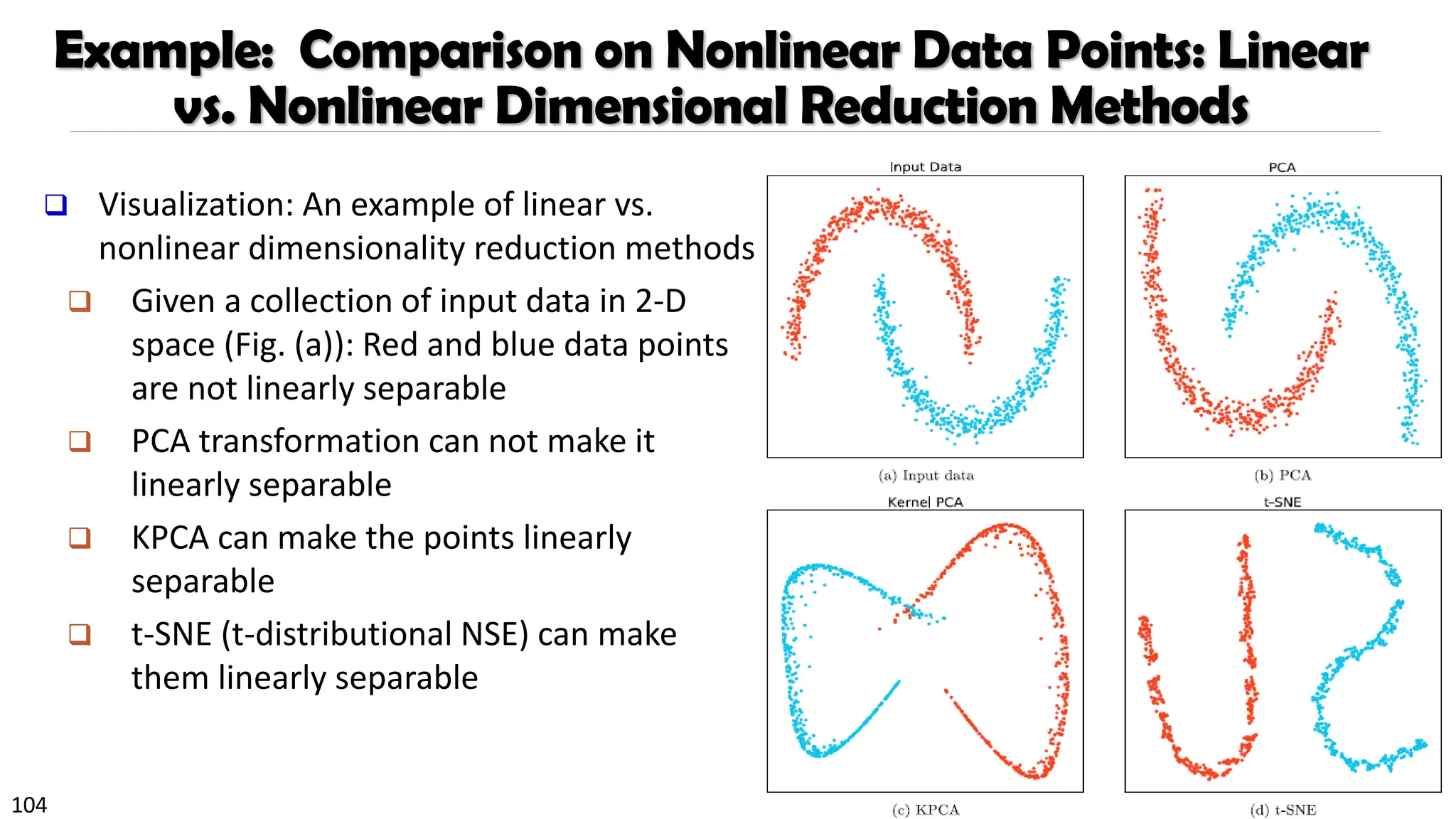
Example: Comparison on Nonlinear Data Points: Linear
vs. Nonlinear Dimensional Reduction Methods
❑ Visualization: An example of linear vs.
nonlinear dimensionality reduction methods
❑ Given a collection of input data in 2-D
space (Fig. (a)): Red and blue data points
are not linearly separable
❑ PCA transformation can not make it
linearly separable
❑ KPCA can make the points linearly
separable
❑ t-SNE (t-distributional NSE) can make
them linearly separable

105
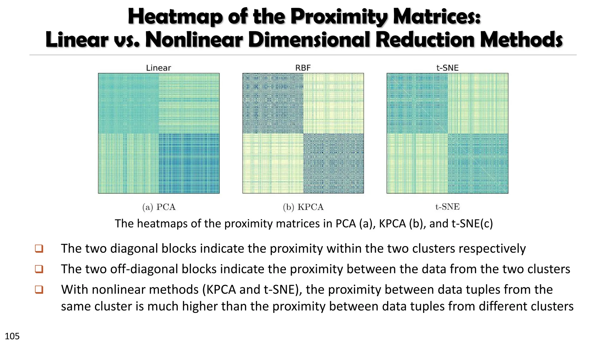
Heatmap of the Proximity Matrices:
Linear vs. Nonlinear Dimensional Reduction Methods
❑ The two diagonal blocks indicate the proximity within the two clusters respectively
❑ The two off-diagonal blocks indicate the proximity between the data from the two clusters
❑ With nonlinear methods (KPCA and t-SNE), the proximity between data tuples from the
same cluster is much higher than the proximity between data tuples from different clusters
The heatmaps of the proximity matrices in PCA (a), KPCA (b), and t-SNE(c)

106
Summary
❑ Data types and attribute types
❑ Nominal, binary, ordinal, numerical, discrete vs. continuous attributes
❑ Statistics of data
❑ Central tendency, dispersion, covariance and correlation, graphical displays
❑ Measure data similarity and correlation
❑ Proximity measures for nominal, binary, numerical, ordinal and mixed types
❑ Cosine similarity
❑ Data quality measures, data cleaning, and data integration
❑ Data transformation: normalization, discretization, data compression and sampling
❑ Dimensionality reduction methodologies
❑ Principal Component Analysis (PCA), attribute subset selection, and nonlinear
dimensionality reduction

Big_DM_24_MS_Topic_02_Understanding Data.pdf

More Related Content

Similar to Big_DM_24_MS_Topic_02_Understanding Data.pdf

Recently uploaded

Big_DM_24_MS_Topic_02_Understanding Data.pdf