Introduction and What is SPSS?
What is it used for?
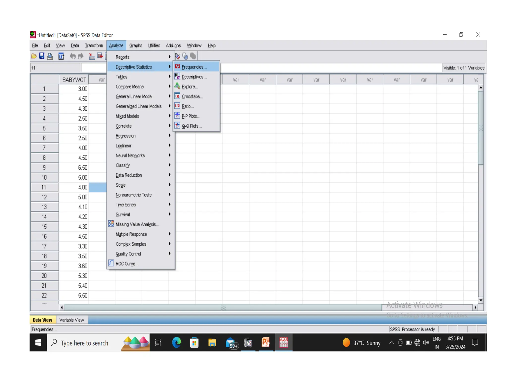
How to Open SPSS?
Basic Structure of SPSS
How to Input Data Manually
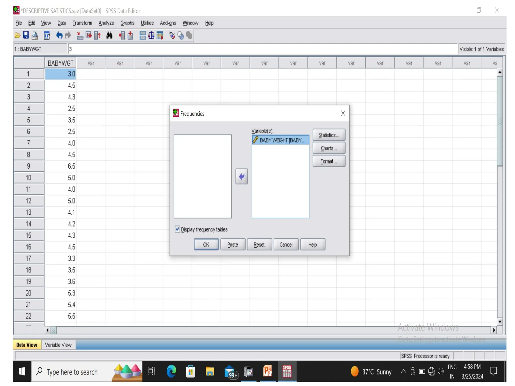
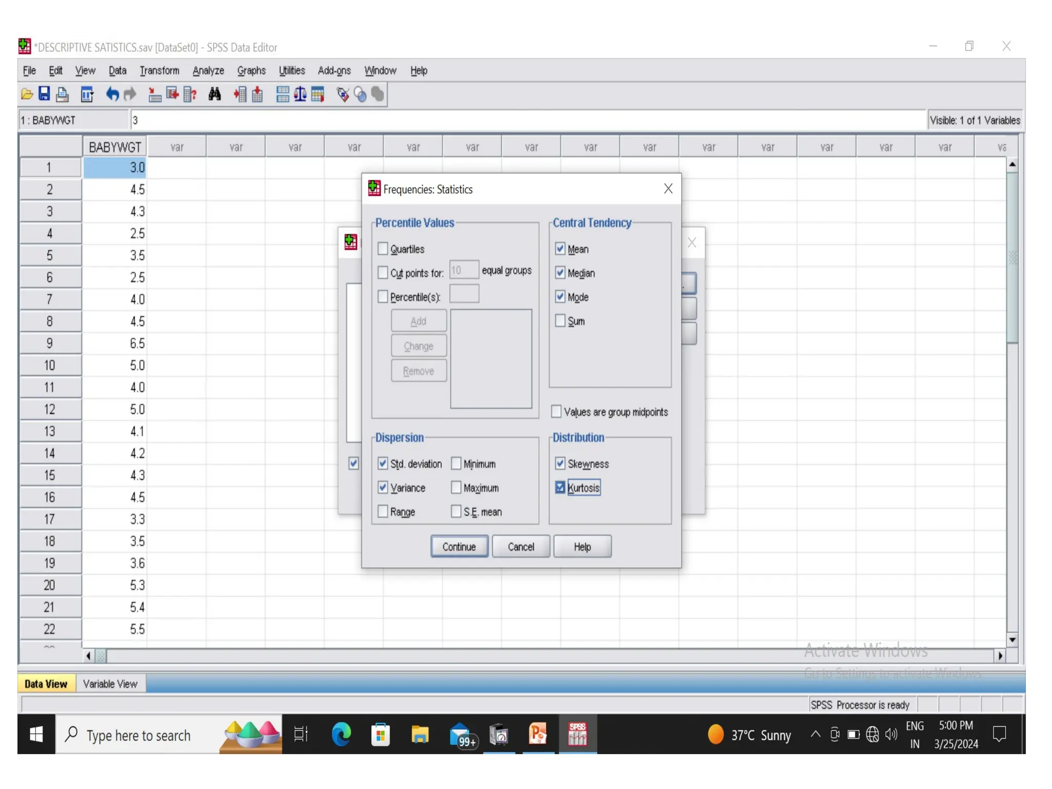
Descriptive Statistics: Mean, Standard Deviation, Frequency
How to perform t-test?
TOPICS COVERED
• Introductionand What is SPSS?
• What is it used for?
• How to Open SPSS?
• Basic Structure of SPSS
• How to Input Data Manually
• Descriptive Statistics: Mean, Standard
Deviation, Frequency
• How to perform t-test?
3.
INTRODUCTION
• SPSS isa Windows based program that can be
used to perform data entry and analysis and to
create tables and graphs.
• SPSS is capable of handling large amounts of
data and can perform all of the analyses covered
in the text and much more.
• SPSS is commonly used in the Social Sciences
and in the business world, so familiarity with this
program should serve you well in the future.
4.
INTRODUCTION
• First versionof SPSS was released in 1968, after
being developed by Norman H. Nie, Dale H.
Bent and Hadlai Hull..
• It was acquired by IBM on July 28, 2009 .
• IBM SPSS Statistics 21.0- Released on August
2012 Latest version.
5.
WHAT IS ITUSED FOR
With SPSS we can analyze data in three basic
ways:
• Describe data using descriptive statistics
• Examine relationship between variables
• Compare groups to determine if there are
significant difference between groups
6.
Basic Structure ofSPSS
There are two different windows in SPSS
• Data Editor Window: Here we can create
variables, enter data and carry out statistical
functions.
• Output Viewer Window: Here the results are
produced by analyzing the functions.
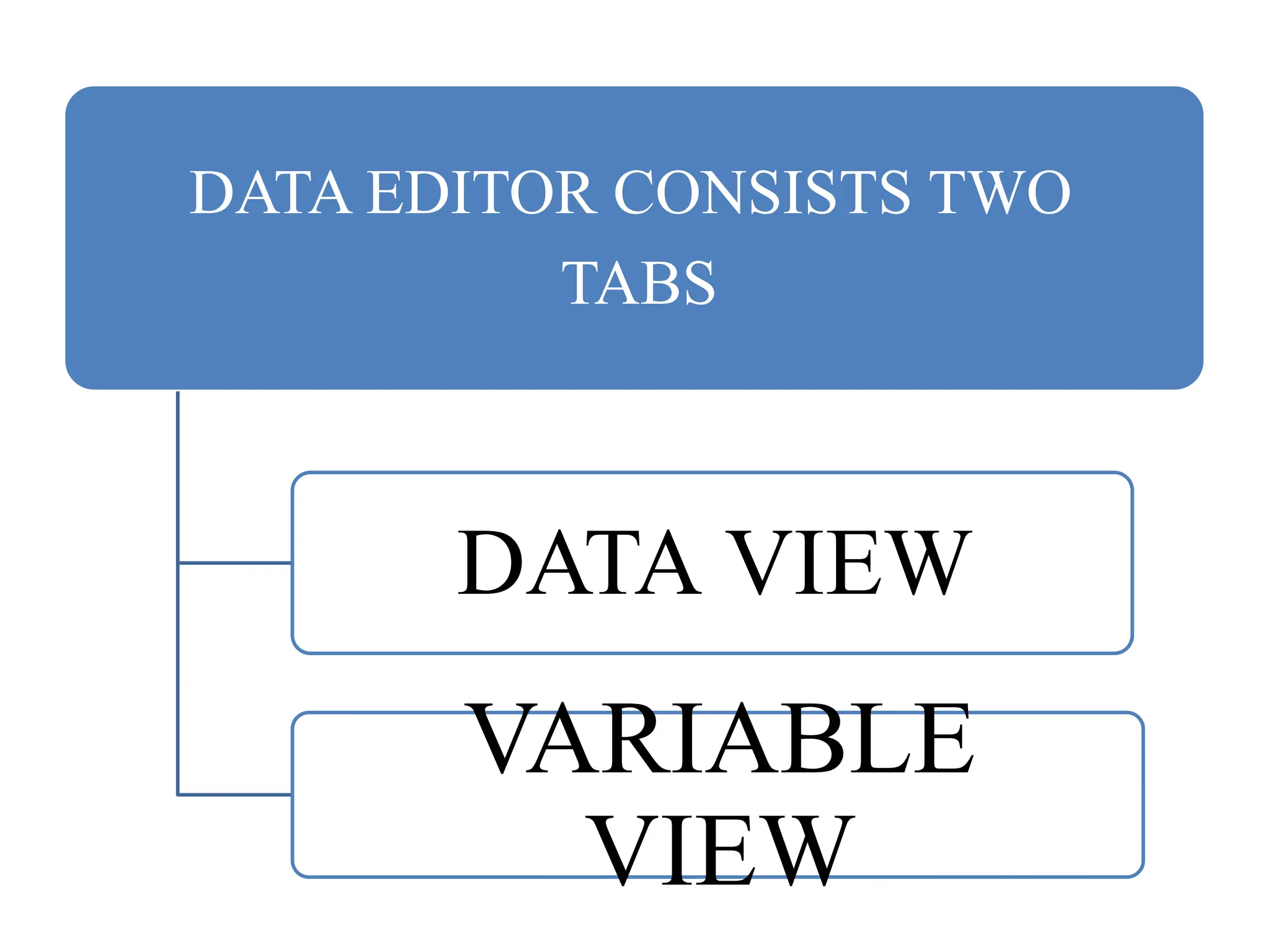
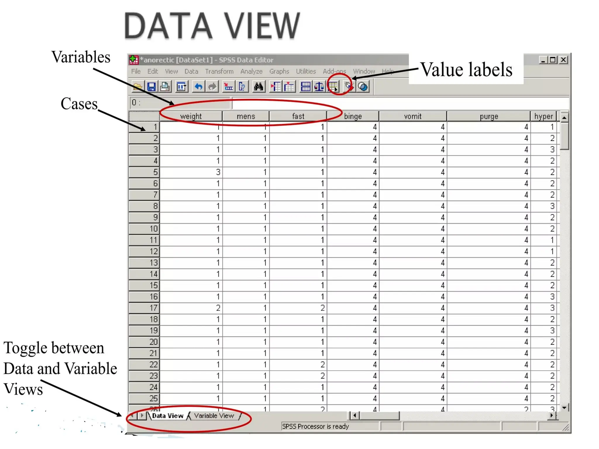
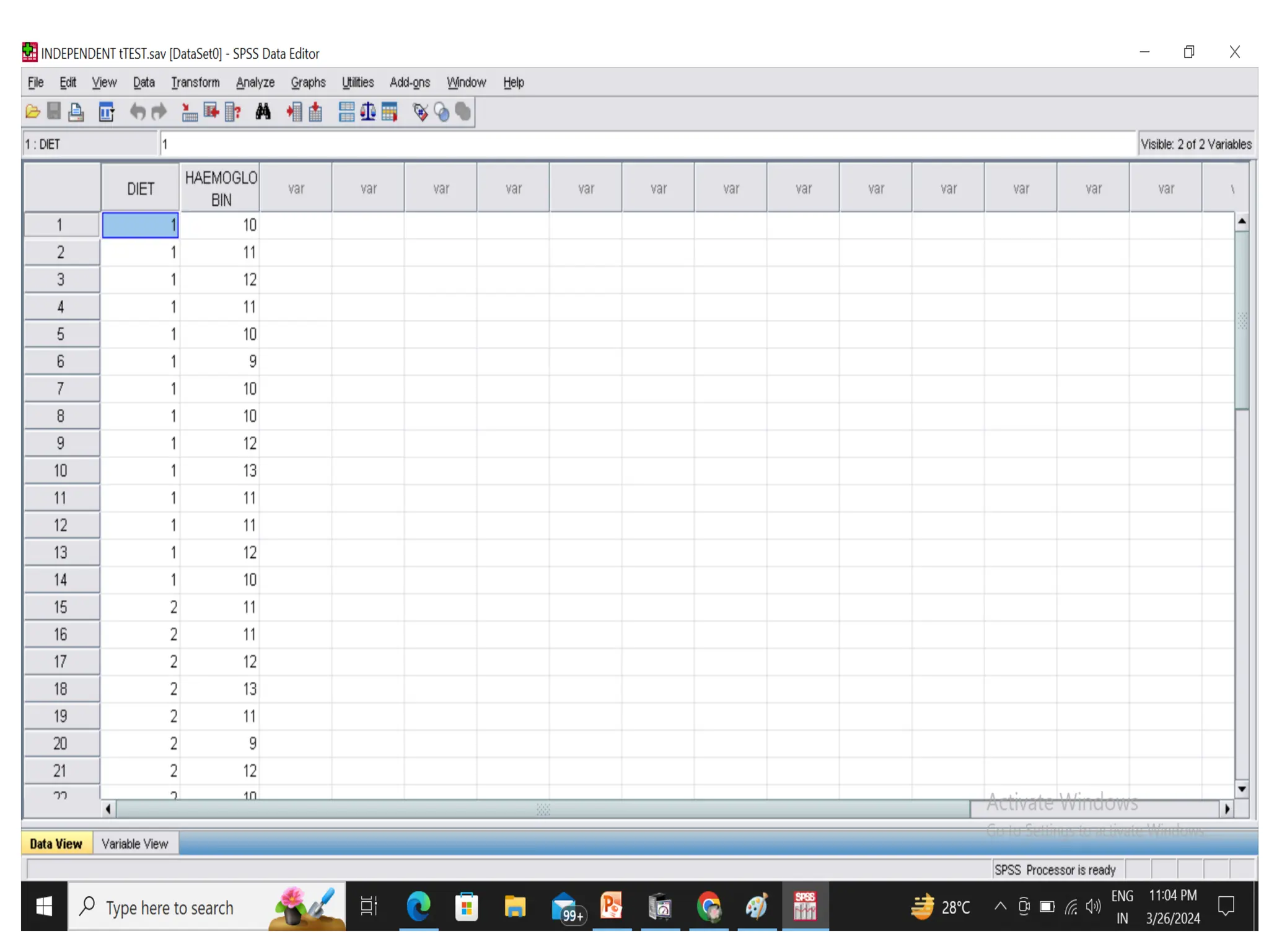
DATA VIEW
Date viewis used to enter data and view data
In data view:
• Row represent individual cases.
• Columns represent particular variable in your
data file.
11.
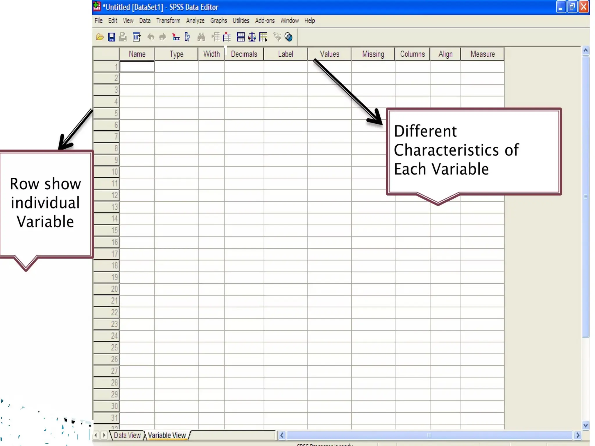
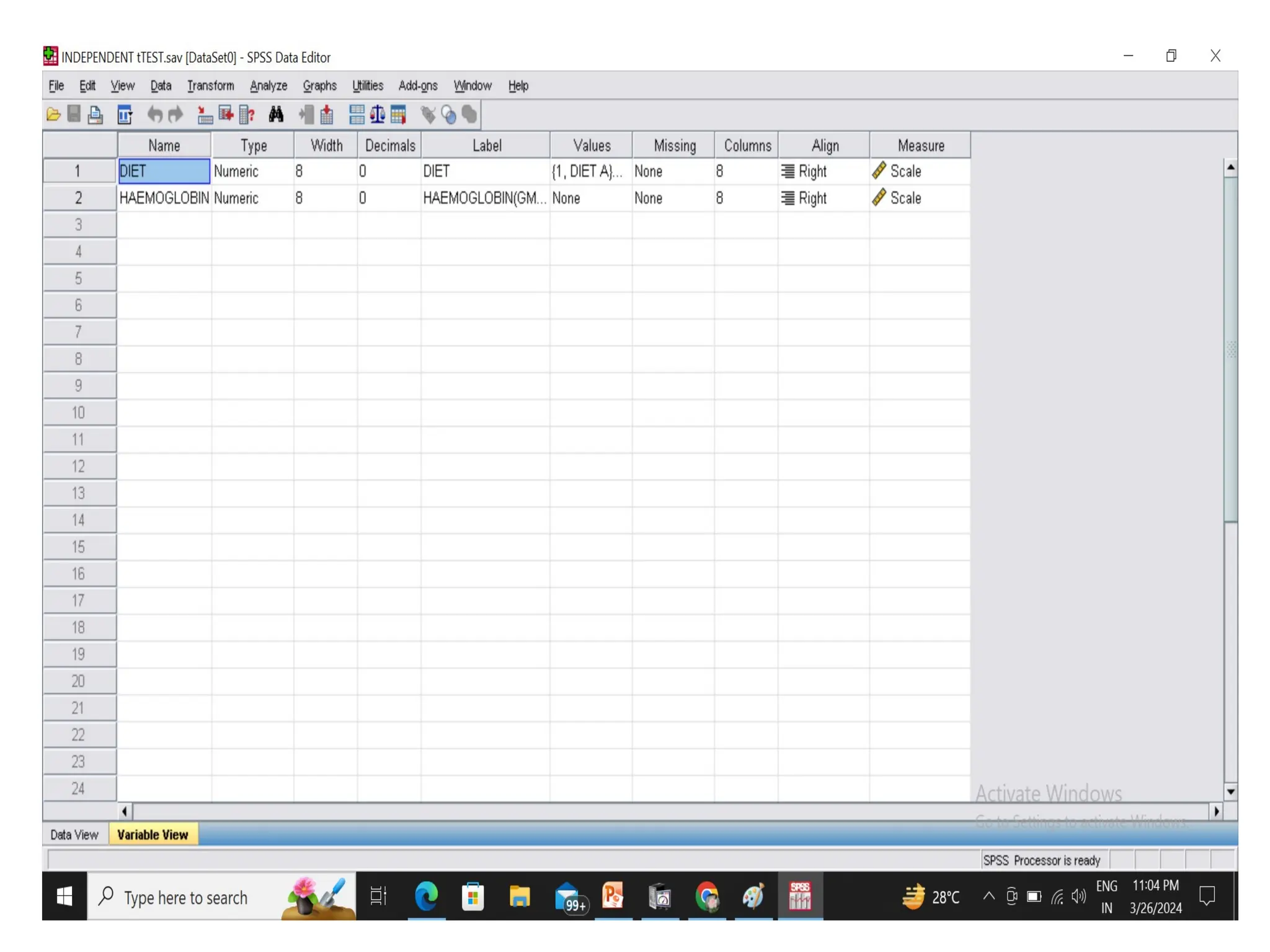
VARIABLE VIEW
Variable viewis used to create and define
various variables:
In Variable View:
• Row represent individual variable or define the
variable
• Column represent the specific characteristic of
variable like Name, Type, Width, Decimals,
Label, Missing, Align, Measure.
13.
VARIABLES
A concept whichcan take on different
quantitative values is called a variable.
What are variables you would consider in buying
a second hand bike?
Brand
Type
Age
Condition(Excellent, good, poor)
Price
14.
• Dichotomous variables( having two values only)
Yes or No
Male or Female
• Continuous Variables may take on any value
within a given range, or in some cases, an
infinite set.
Income
age
a test score
15.
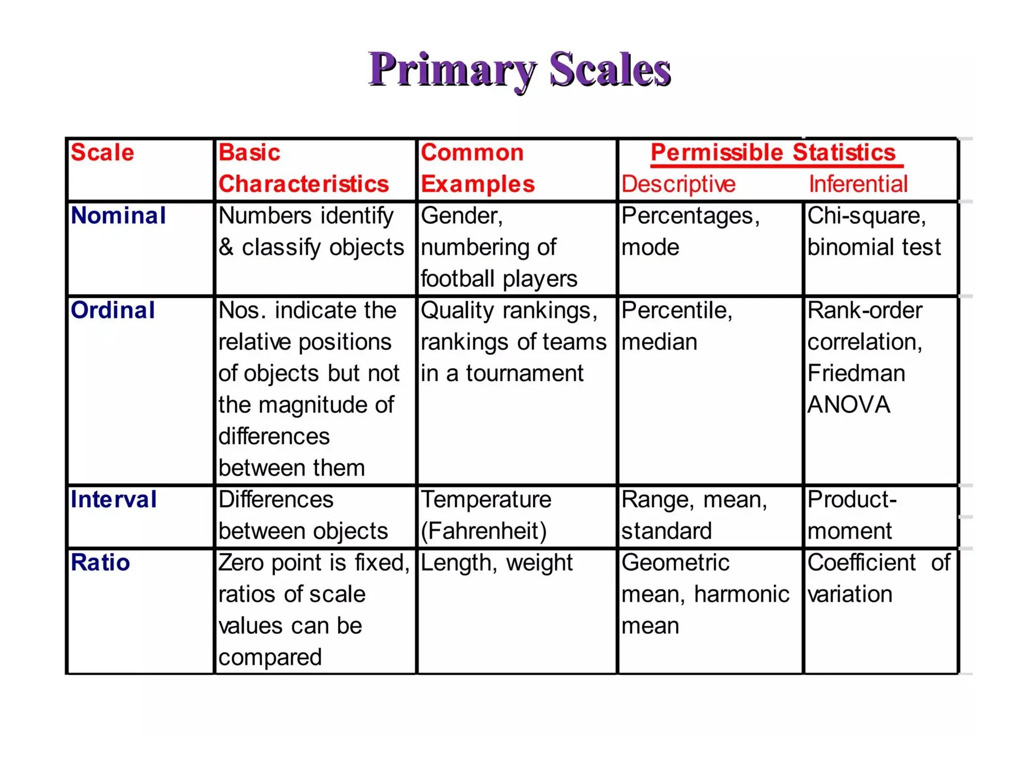
Measurement Scales
The processof assigning numbers to objects in
such a way that specific properties of the objects
are faithfully represented .
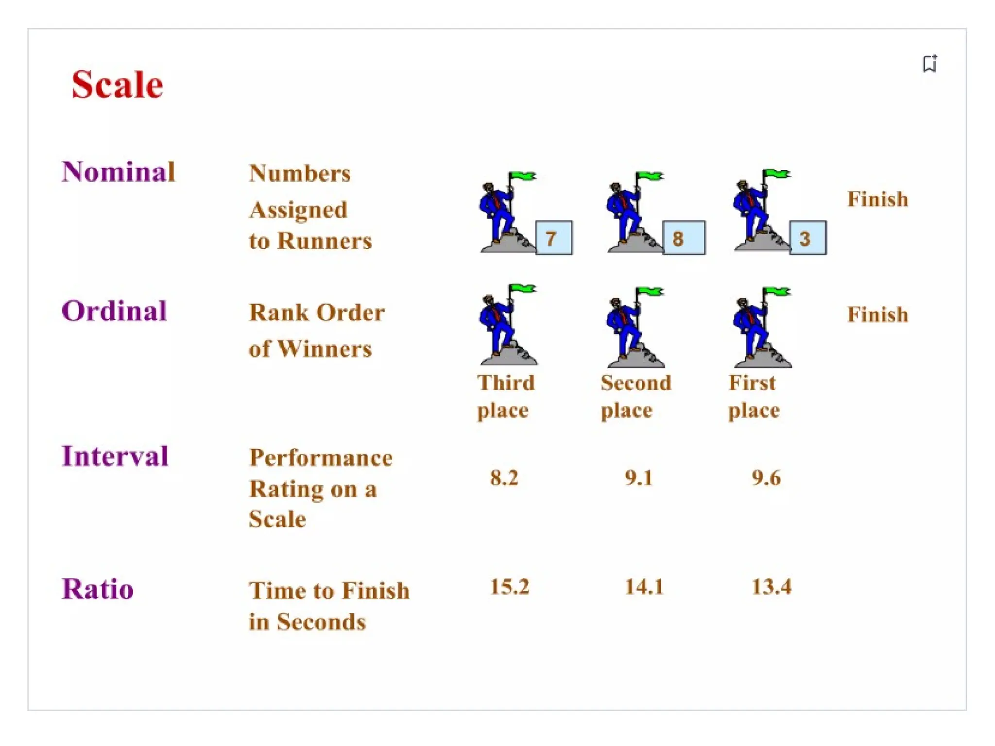
Types of Scales:
Nominal
Ordinal
Scale
Interval
Ratio
16.
Types of Scales
NominalScale:
is defined as a scale that labels variables
into distinct classifications and doesn’t involve a
quantitative value or order. This scale is the
simplest of the four variable measurement scales.
Examples
• Gender
• Political preferences
• Place of residence
17.
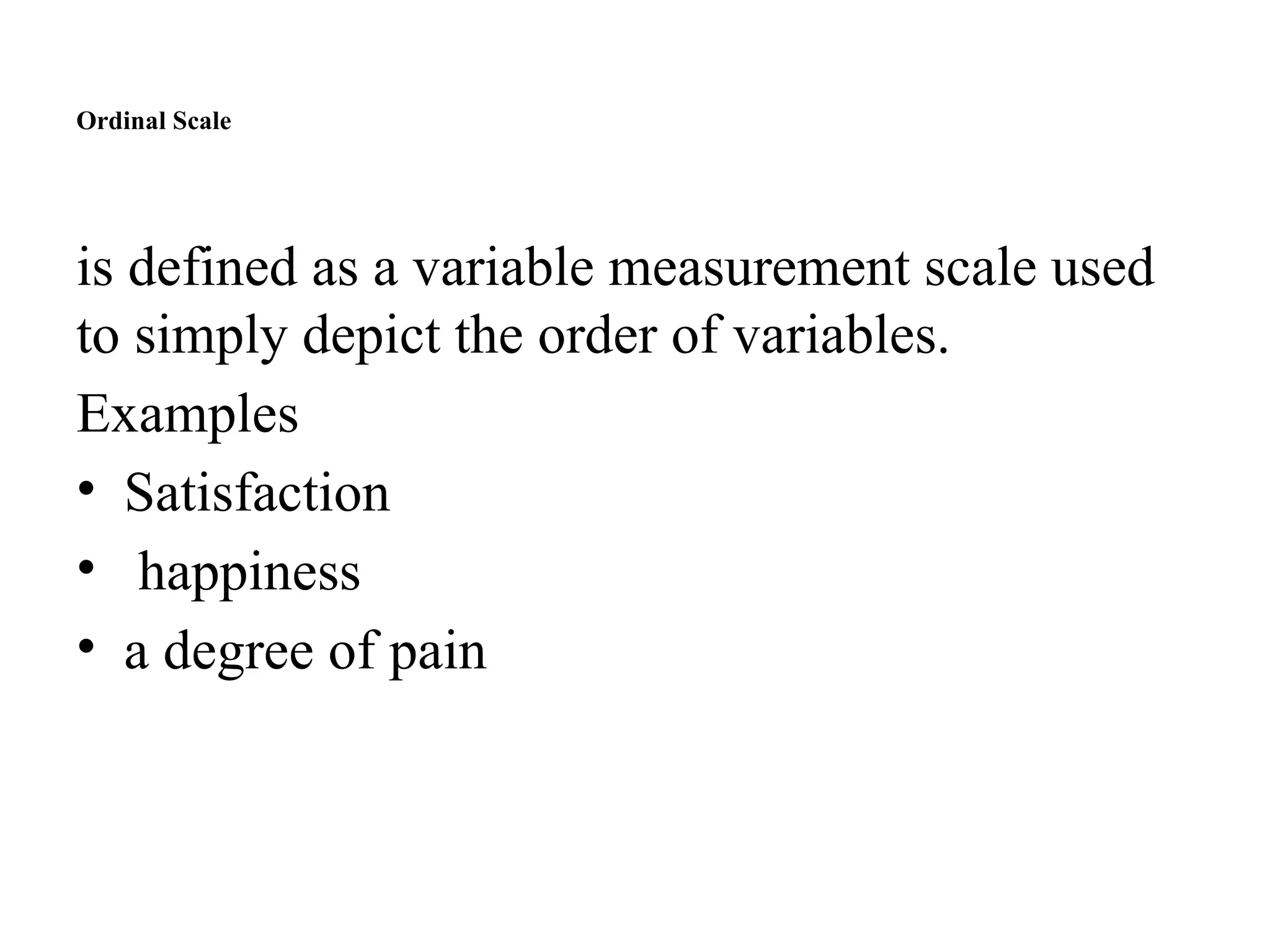
Ordinal Scale
is definedas a variable measurement scale used
to simply depict the order of variables.
Examples
• Satisfaction
• happiness
• a degree of pain
18.
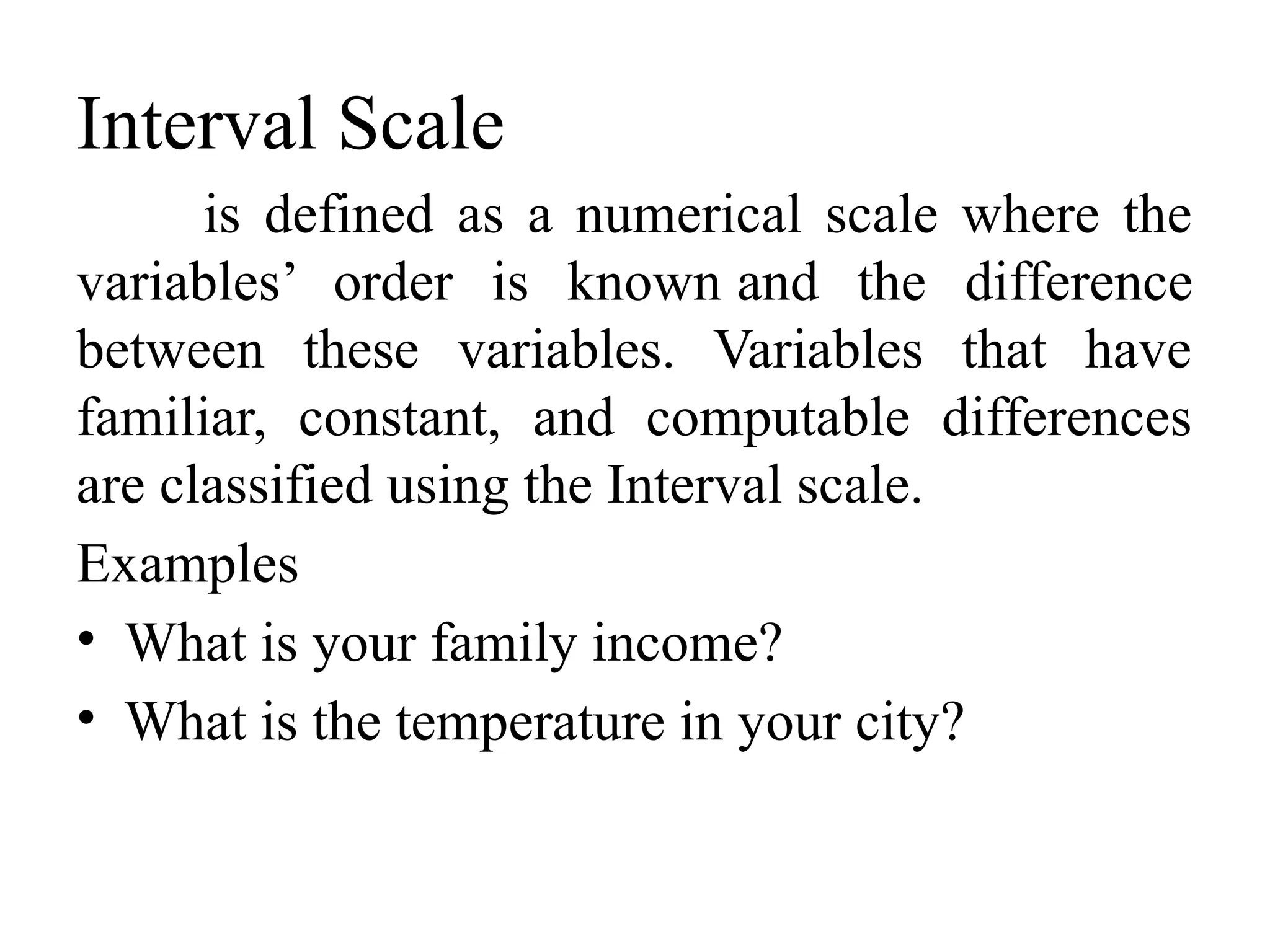
Interval Scale
is definedas a numerical scale where the
variables’ order is known and the difference
between these variables. Variables that have
familiar, constant, and computable differences
are classified using the Interval scale.
Examples
• What is your family income?
• What is the temperature in your city?
19.
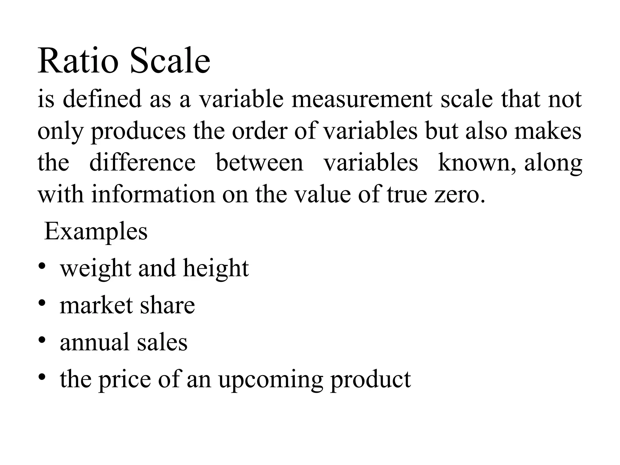
Ratio Scale
is definedas a variable measurement scale that not
only produces the order of variables but also makes
the difference between variables known, along
with information on the value of true zero.
Examples
• weight and height
• market share
• annual sales
• the price of an upcoming product
22.
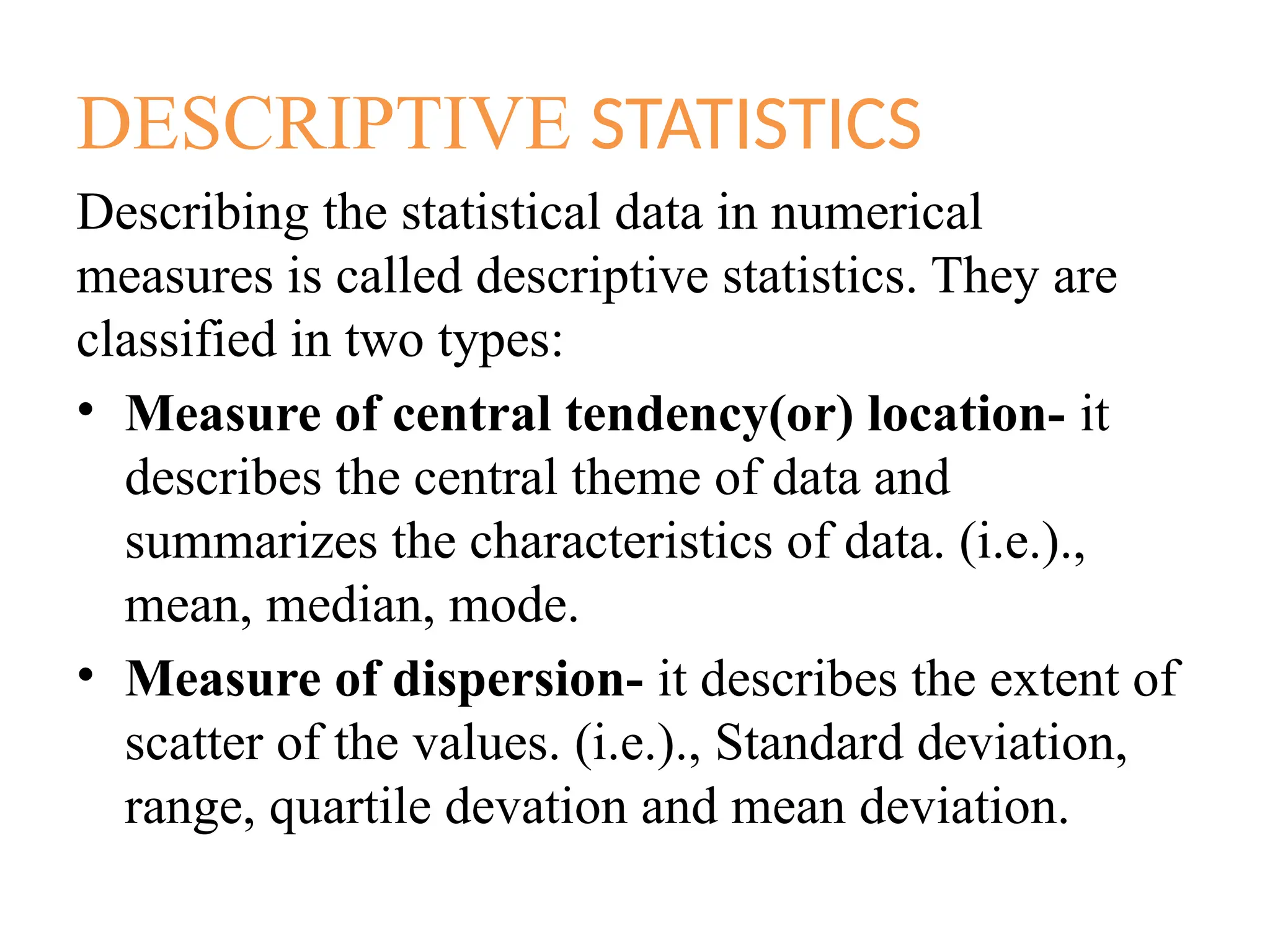
DESCRIPTIVE STATISTICS
Describing thestatistical data in numerical
measures is called descriptive statistics. They are
classified in two types:
• Measure of central tendency(or) location- it
describes the central theme of data and
summarizes the characteristics of data. (i.e.).,
mean, median, mode.
• Measure of dispersion- it describes the extent of
scatter of the values. (i.e.)., Standard deviation,
range, quartile devation and mean deviation.
23.
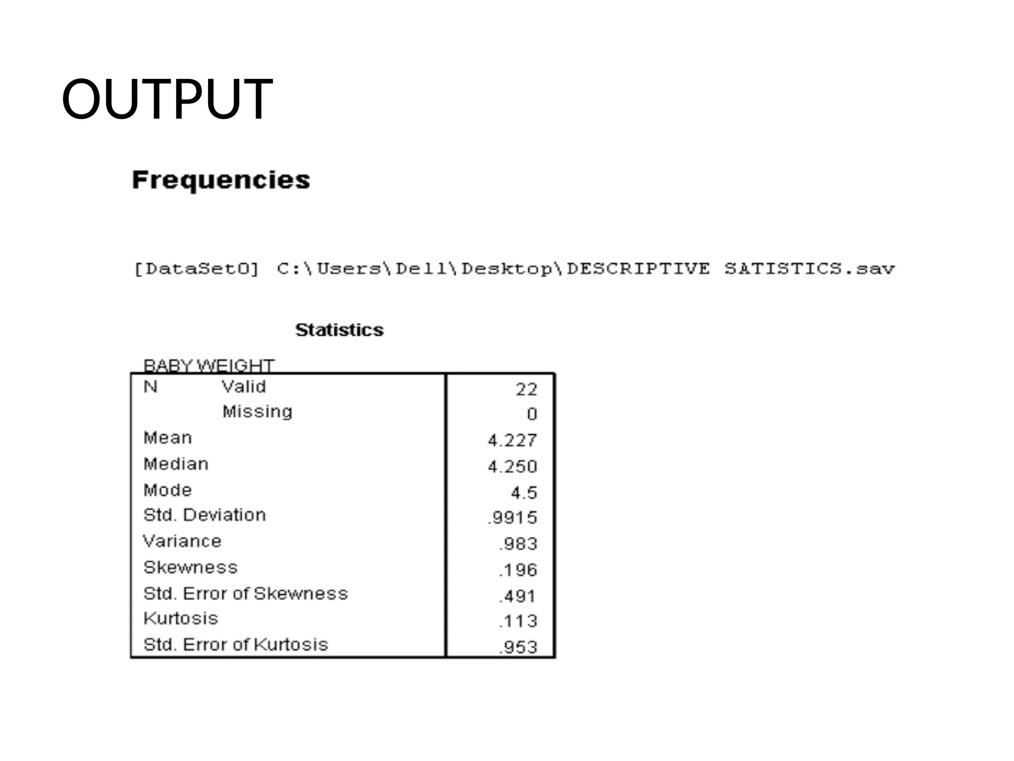
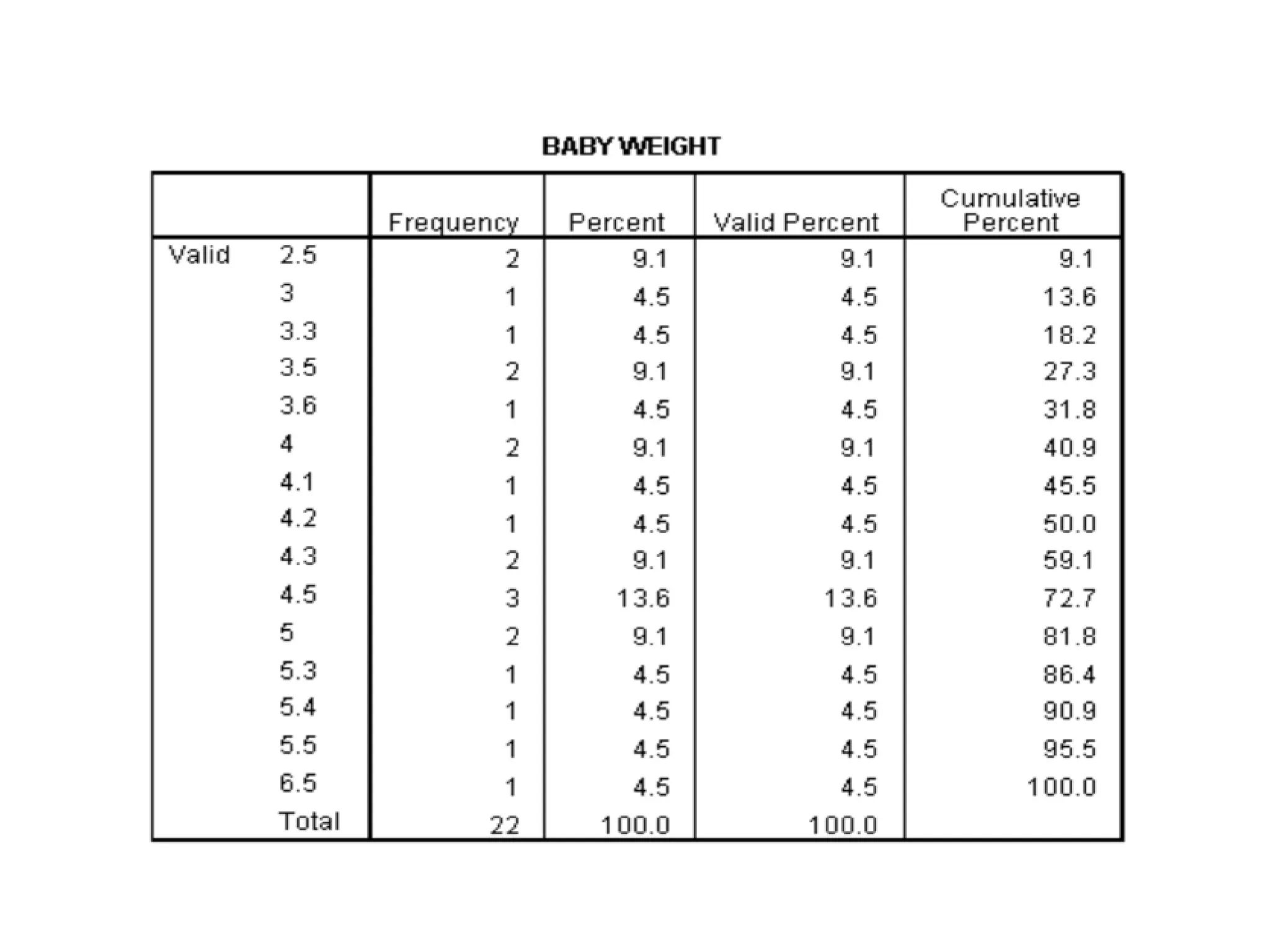
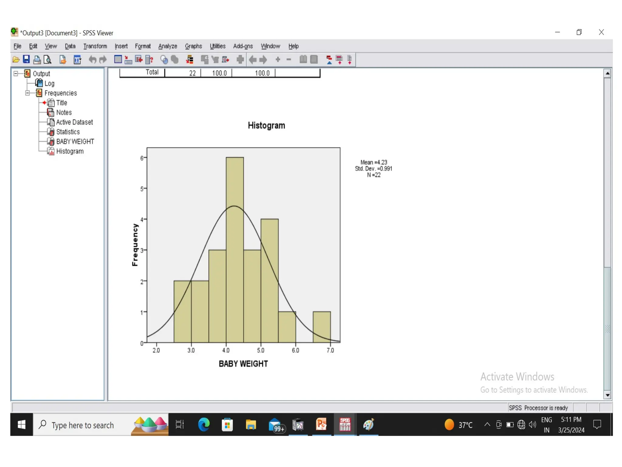
Example:
Weight of babies(kg)below 6 months taken
from a hospital record is given below. Calculate
mean, median, mode, standard deviation.
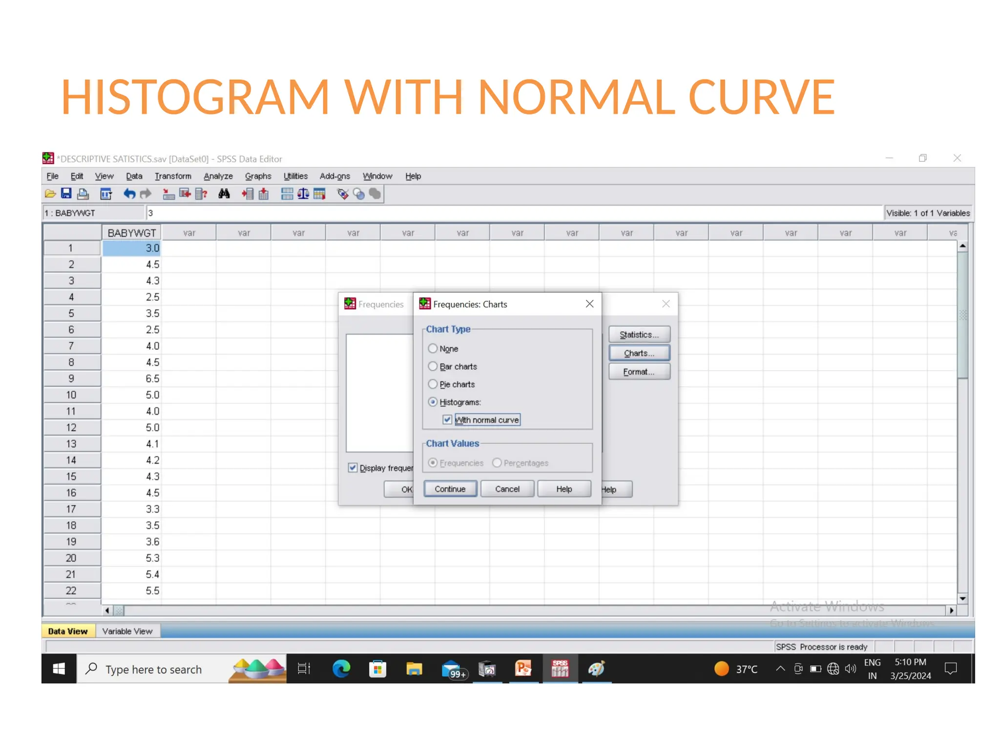
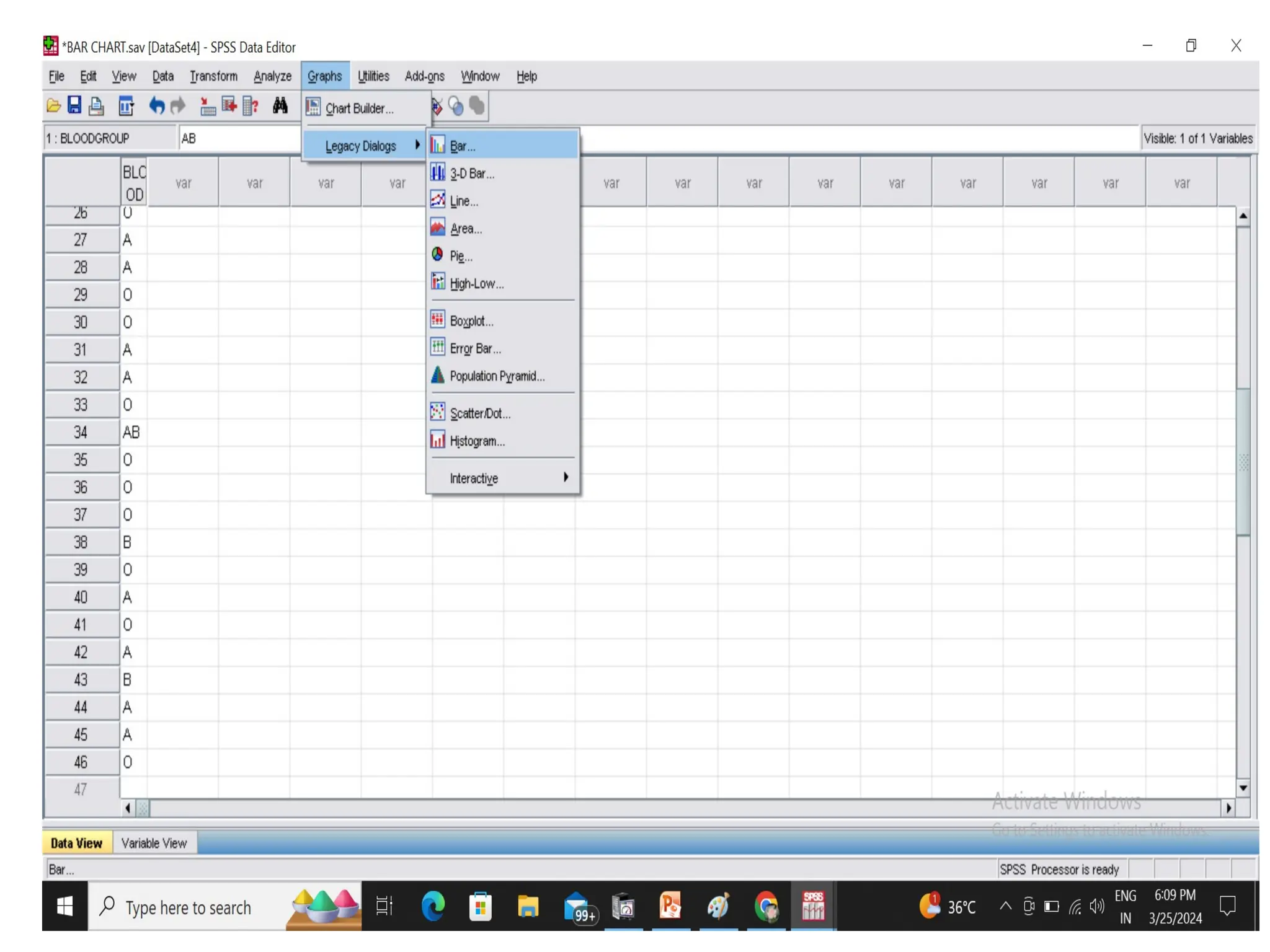
CHARTS IN SPSS
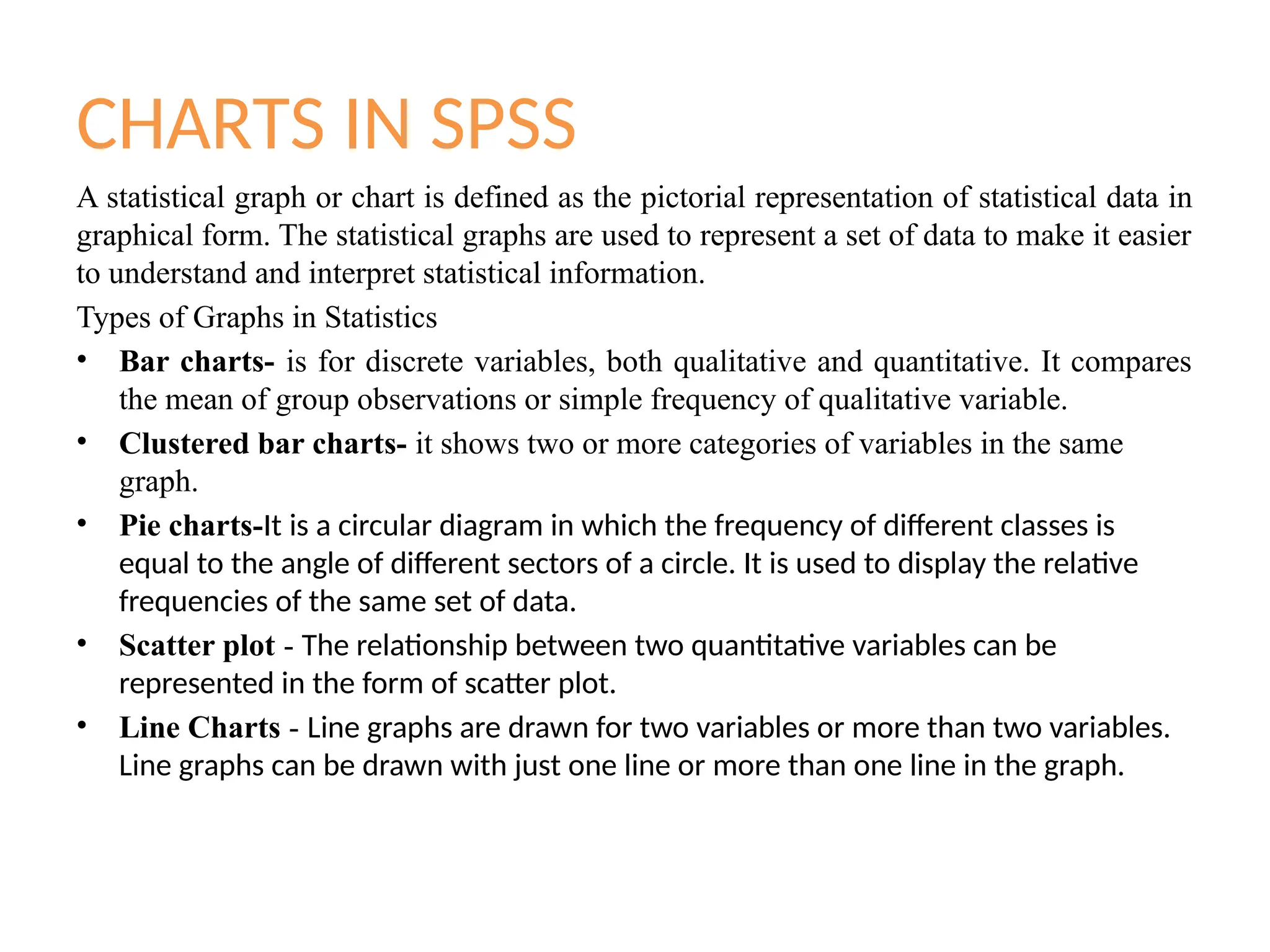
Astatistical graph or chart is defined as the pictorial representation of statistical data in
graphical form. The statistical graphs are used to represent a set of data to make it easier
to understand and interpret statistical information.
Types of Graphs in Statistics
• Bar charts- is for discrete variables, both qualitative and quantitative. It compares
the mean of group observations or simple frequency of qualitative variable.
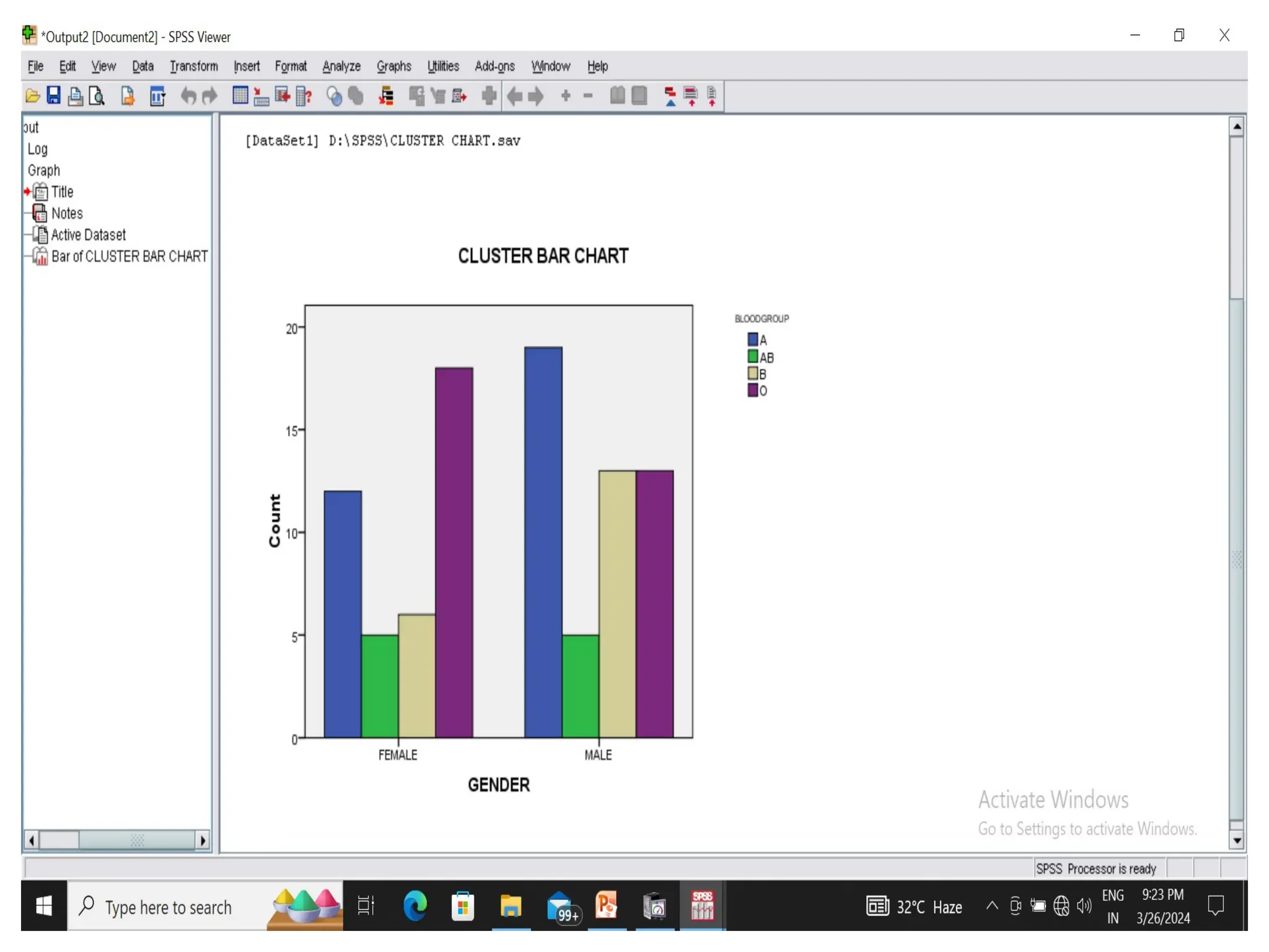
• Clustered bar charts- it shows two or more categories of variables in the same
graph.
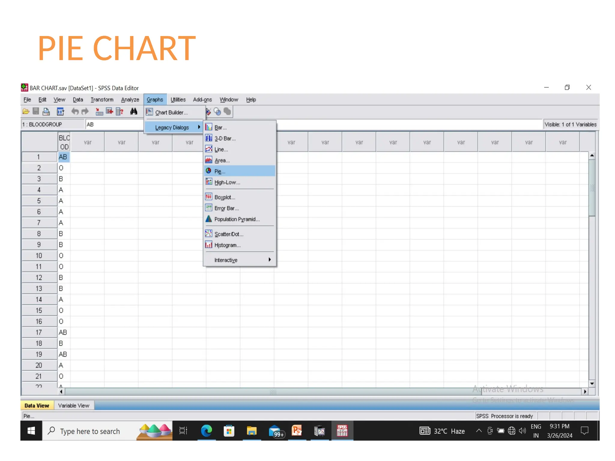
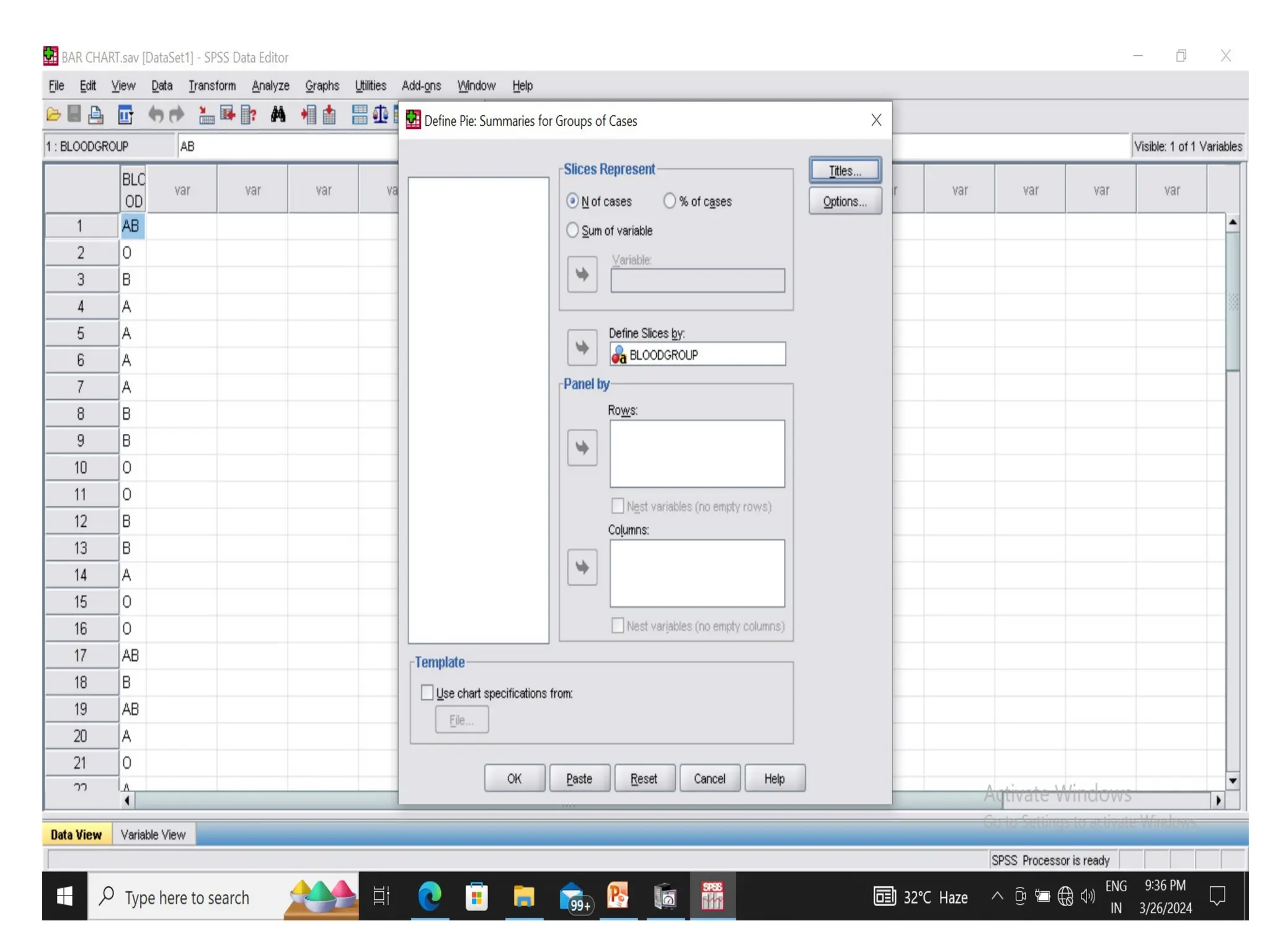
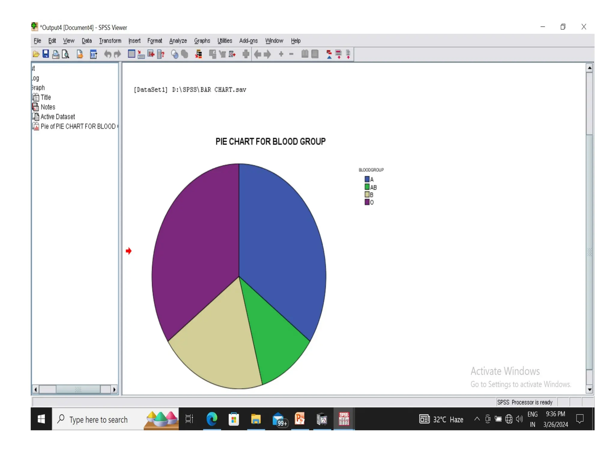
• Pie charts-It is a circular diagram in which the frequency of different classes is
equal to the angle of different sectors of a circle. It is used to display the relative
frequencies of the same set of data.
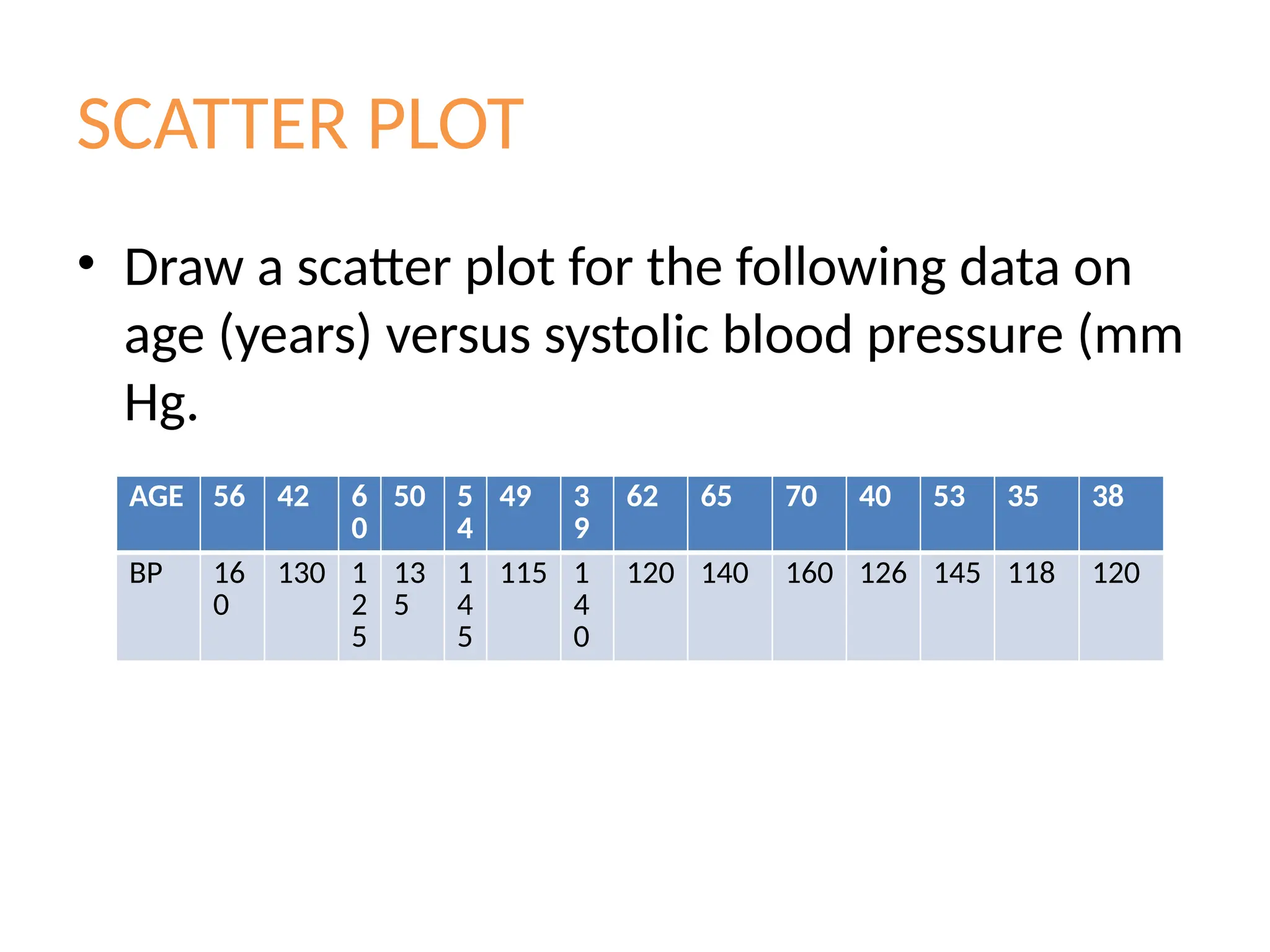
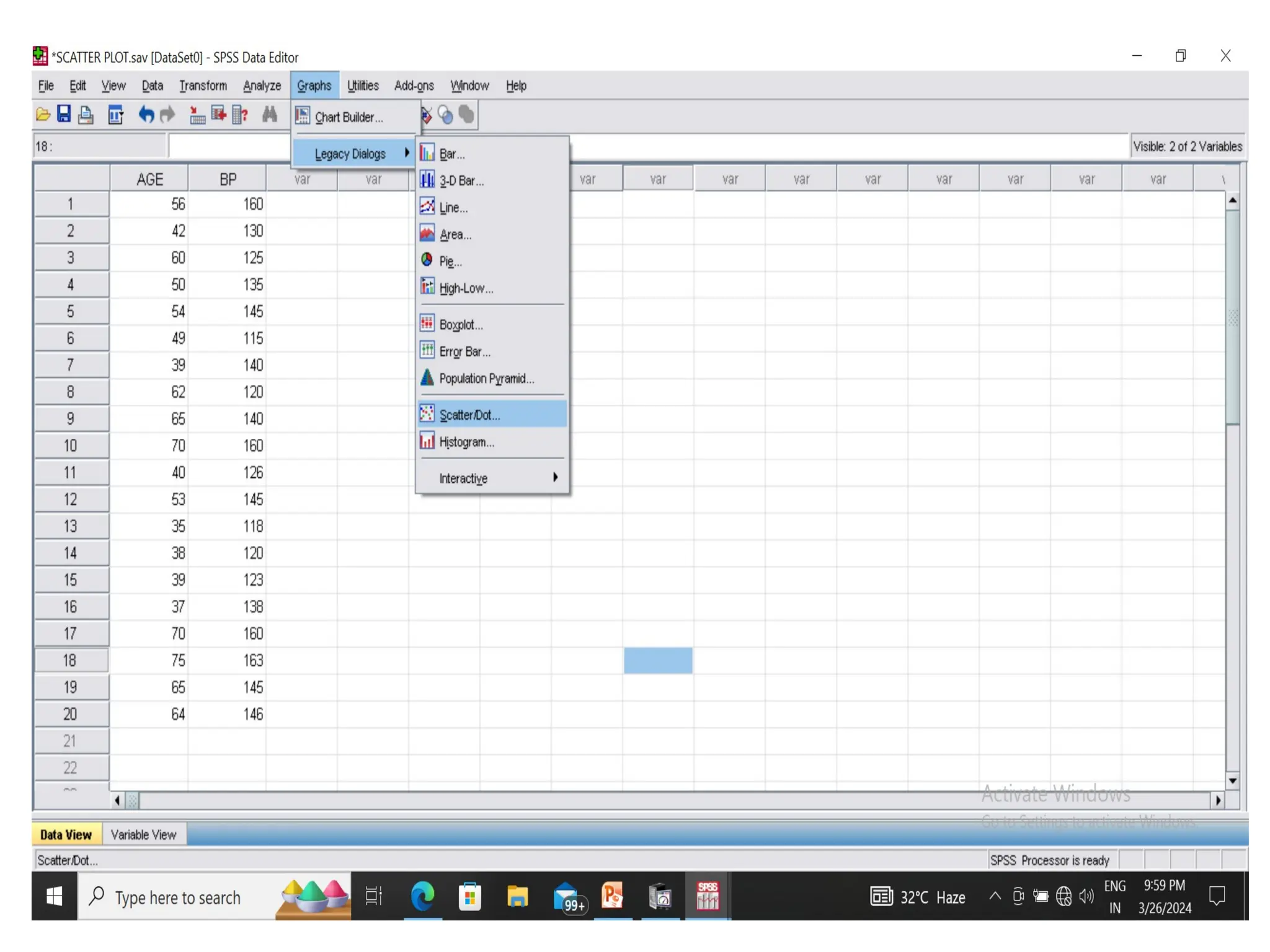
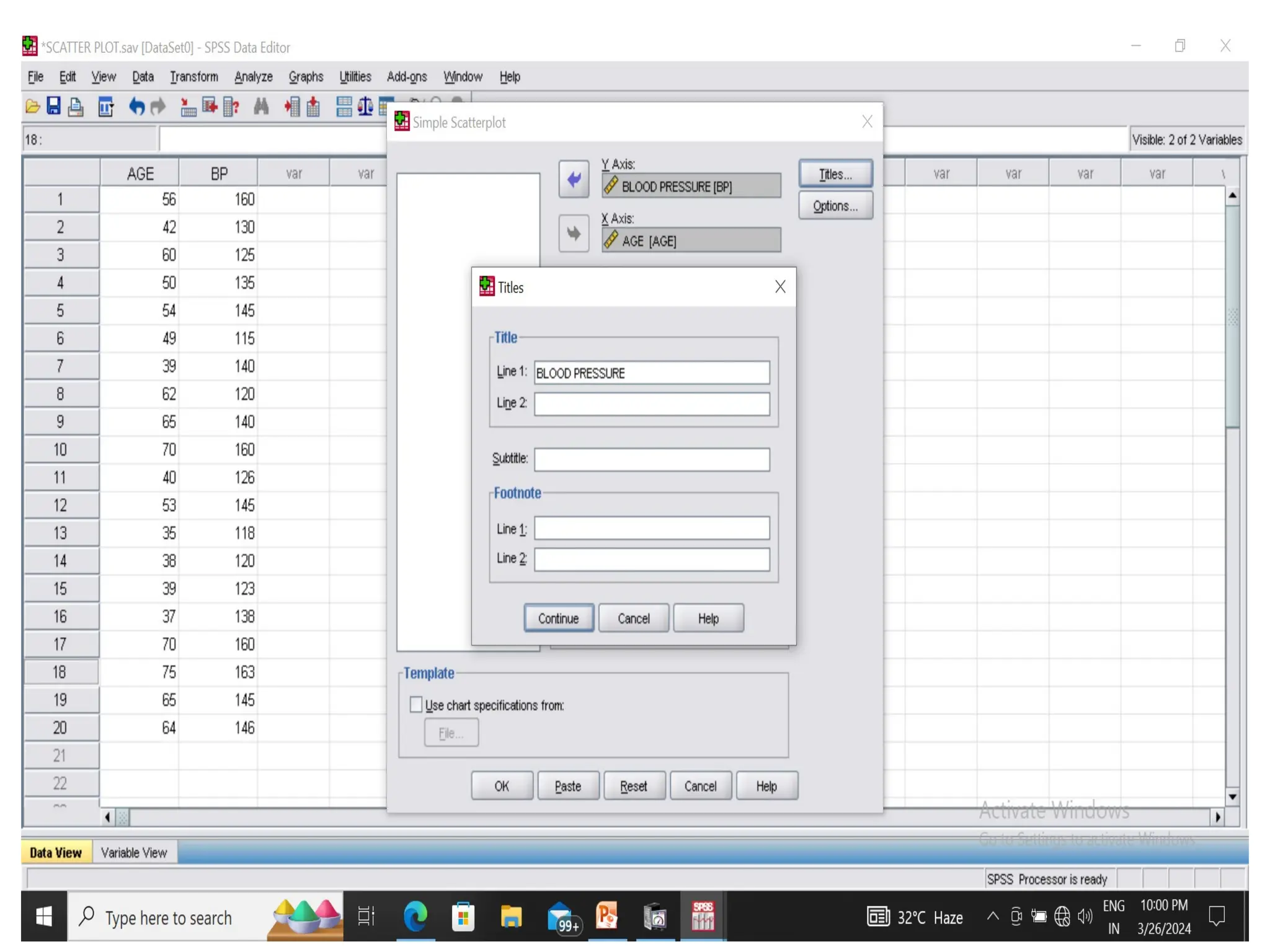
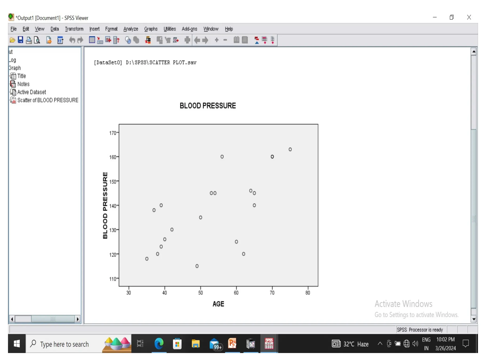
• Scatter plot - The relationship between two quantitative variables can be
represented in the form of scatter plot.
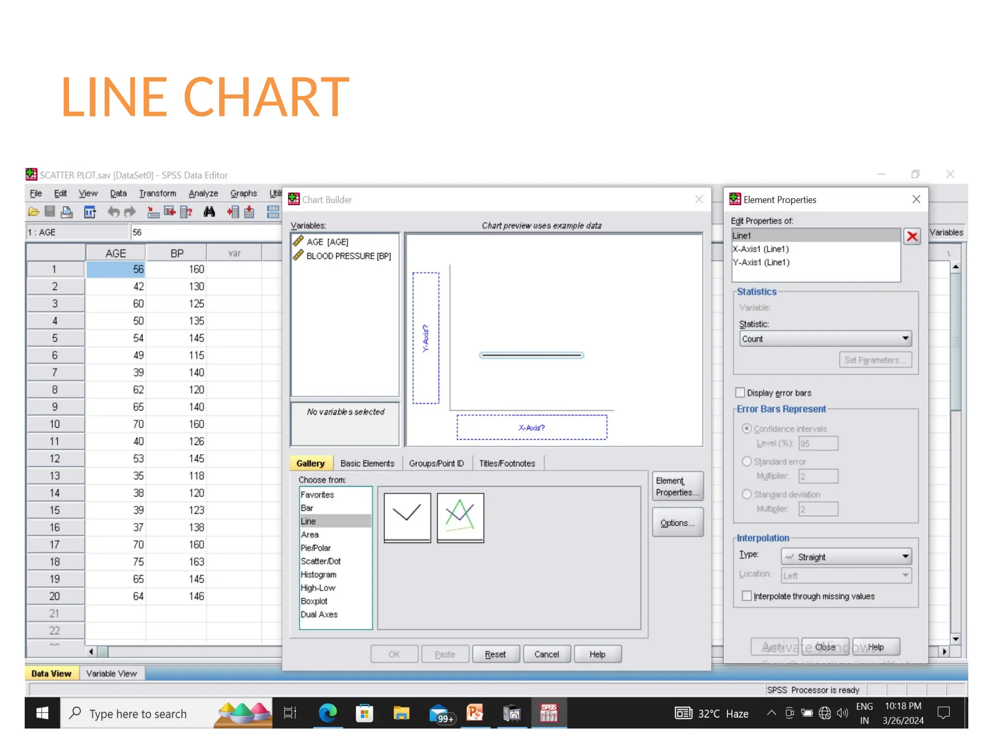
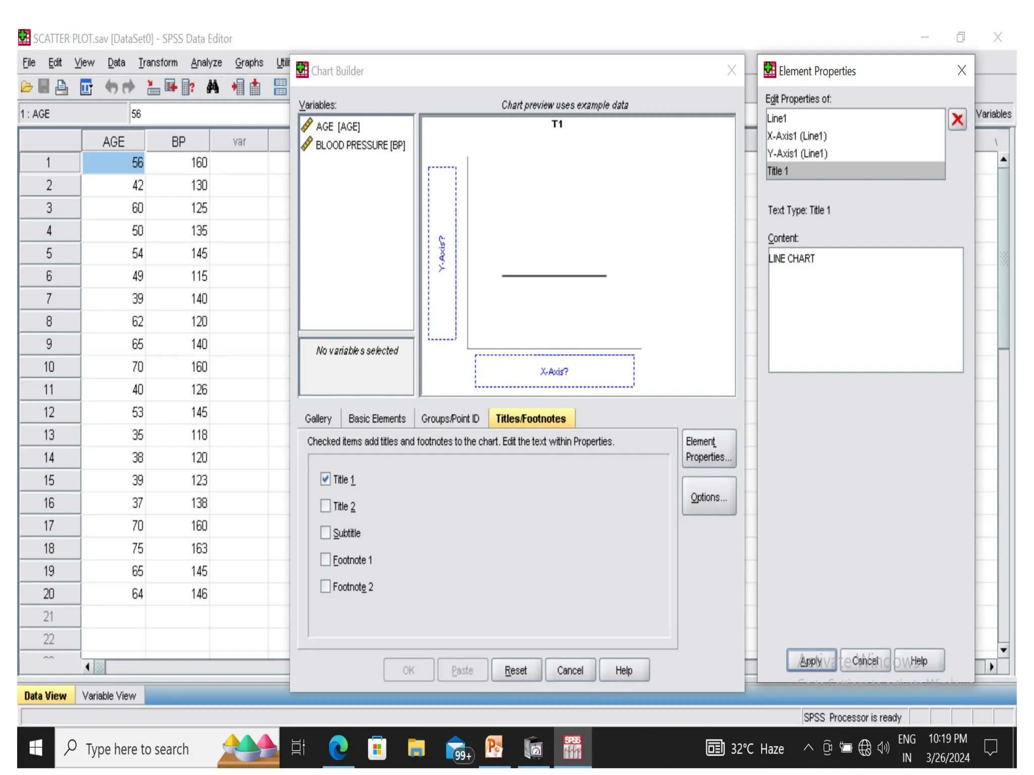
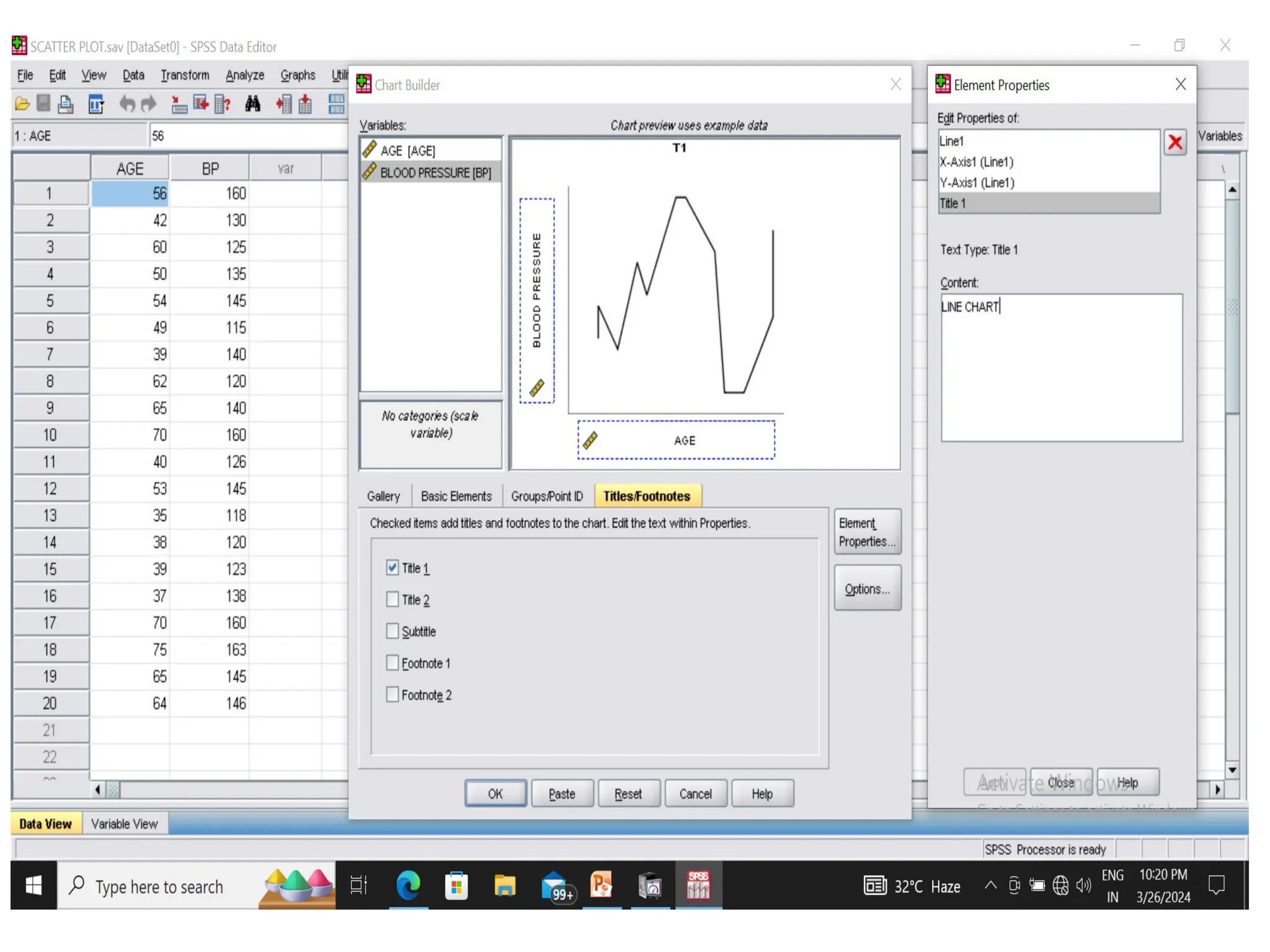
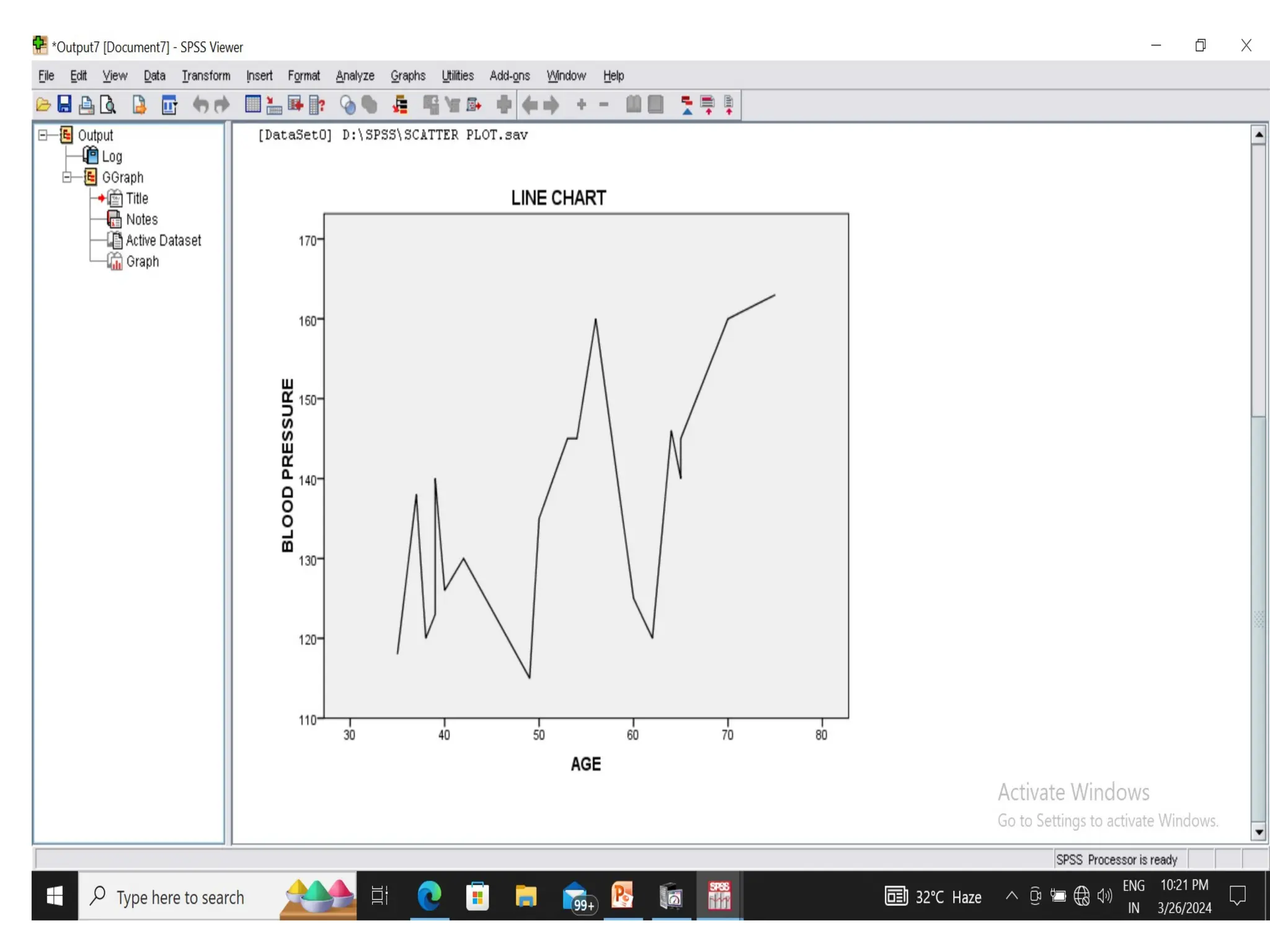
• Line Charts - Line graphs are drawn for two variables or more than two variables.
Line graphs can be drawn with just one line or more than one line in the graph.
32.
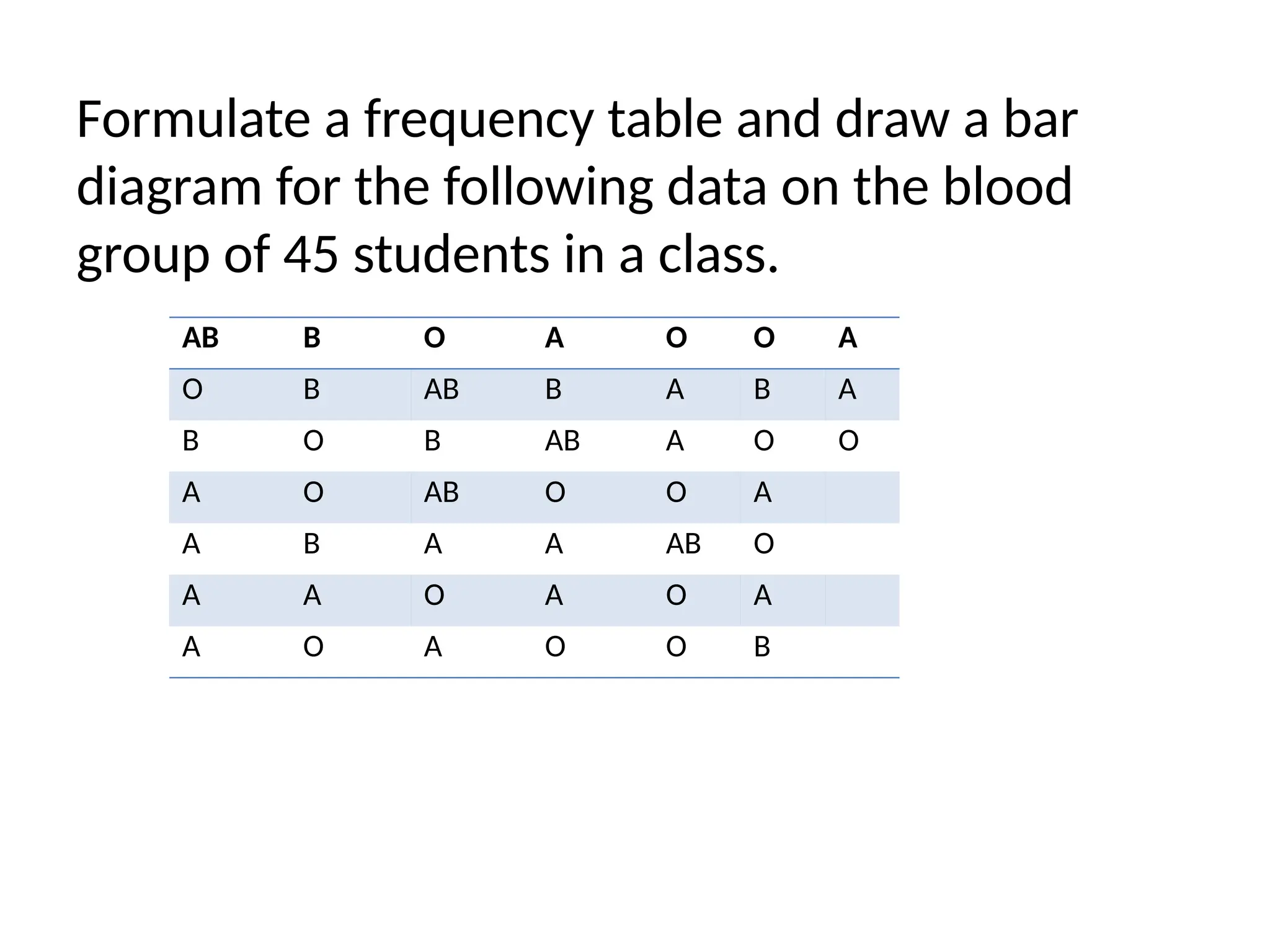
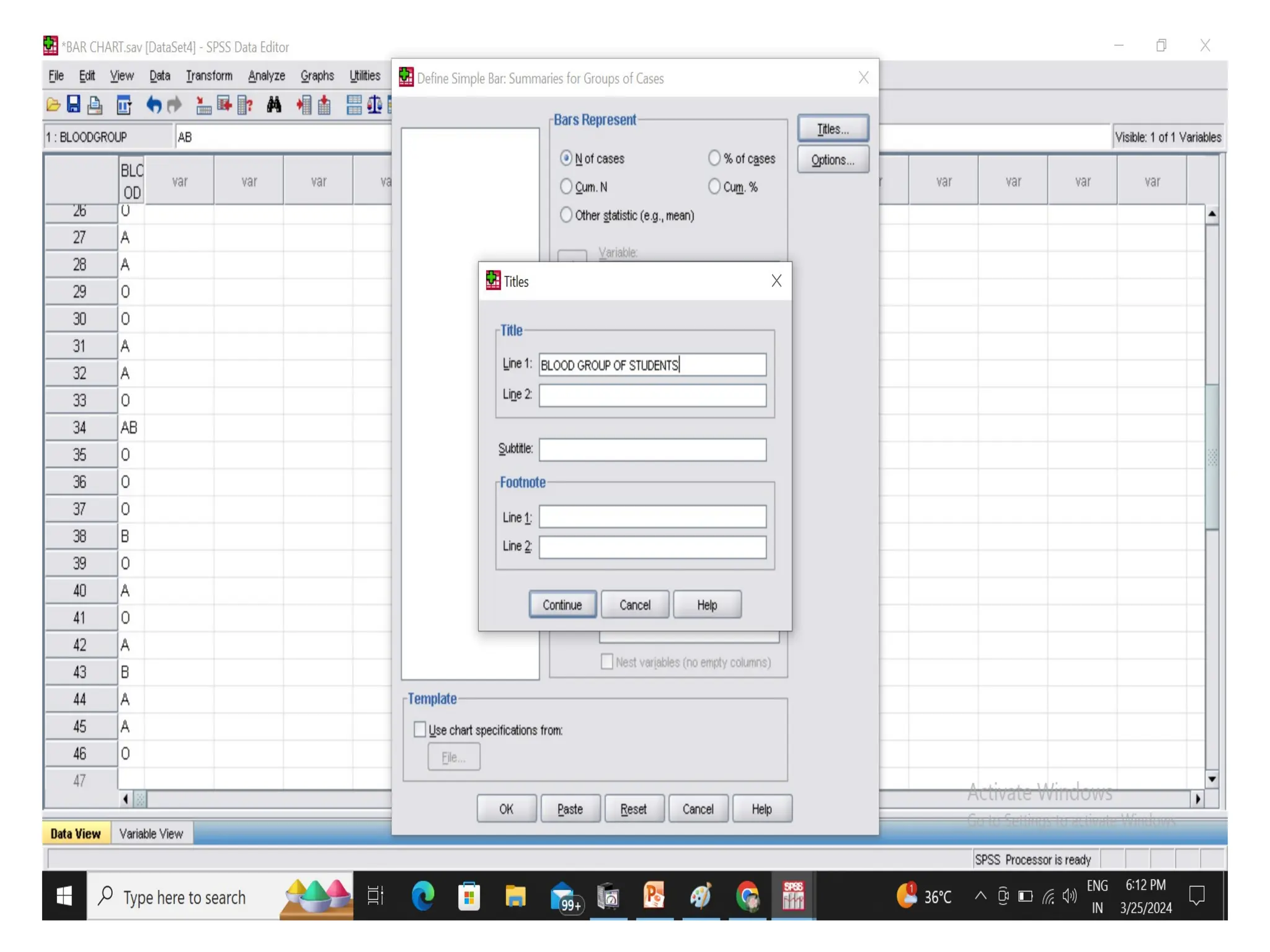
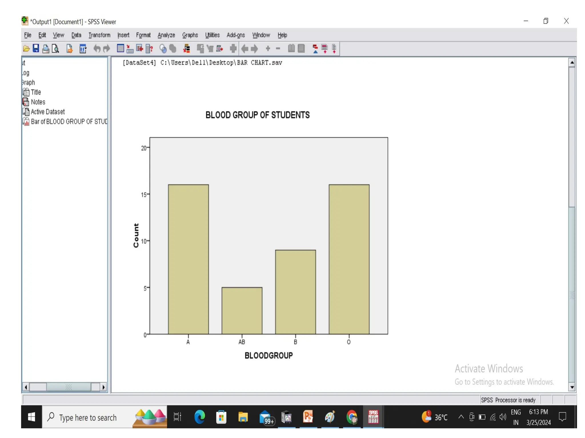
Formulate a frequencytable and draw a bar
diagram for the following data on the blood
group of 45 students in a class.
AB B O A O O A
O B AB B A B A
B O B AB A O O
A O AB O O A
A B A A AB O
A A O A O A
A O A O O B
36.
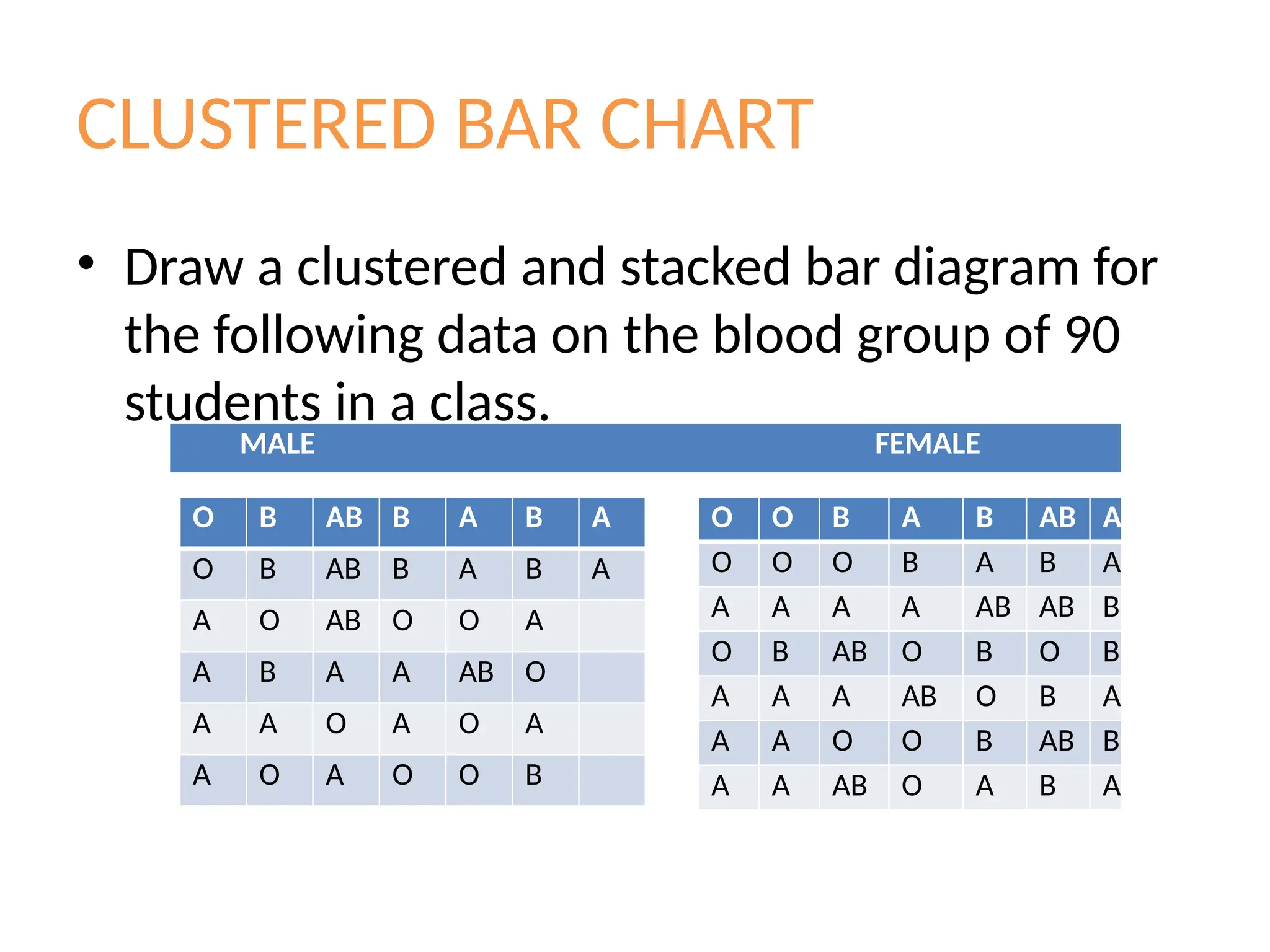
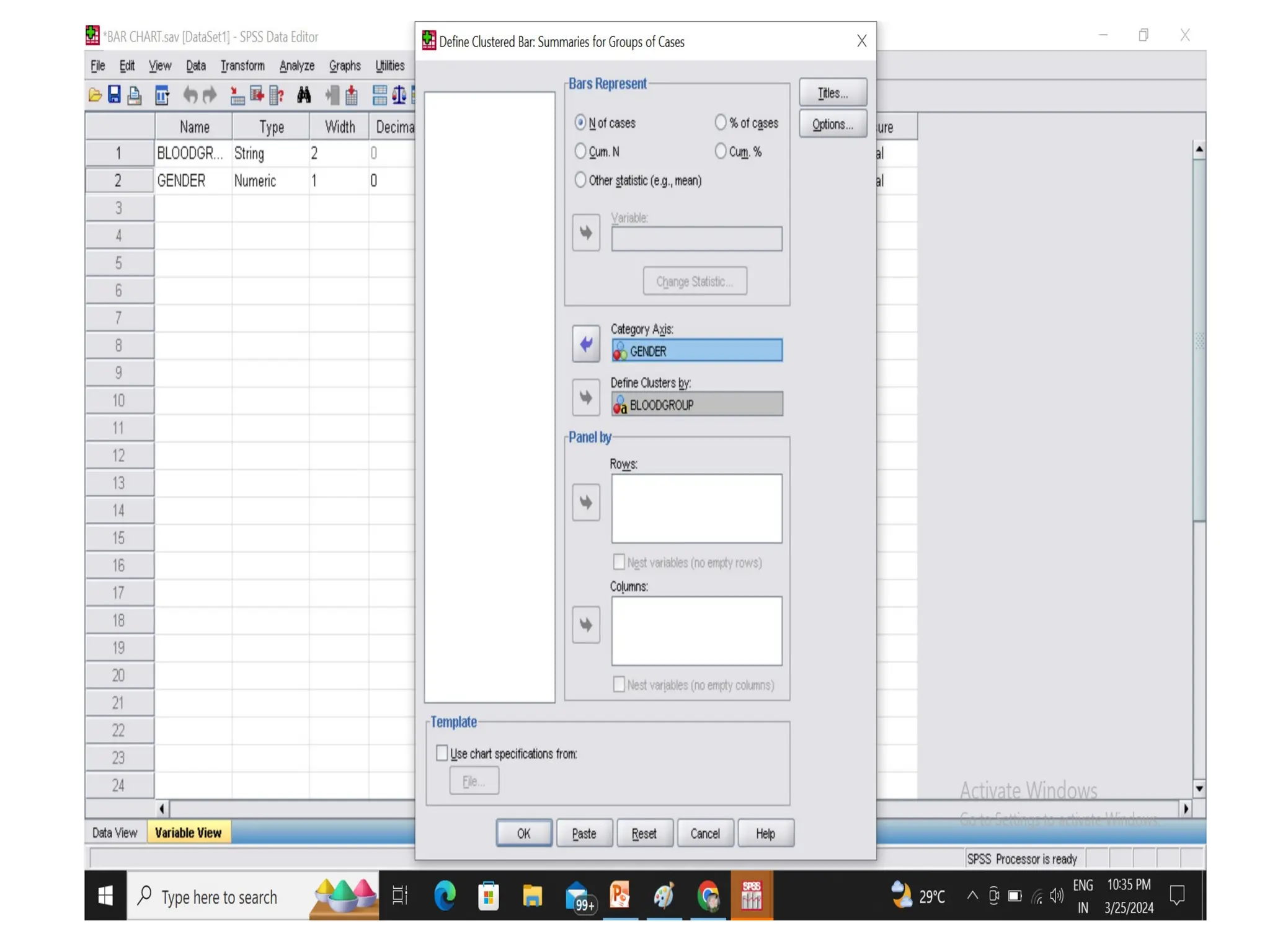
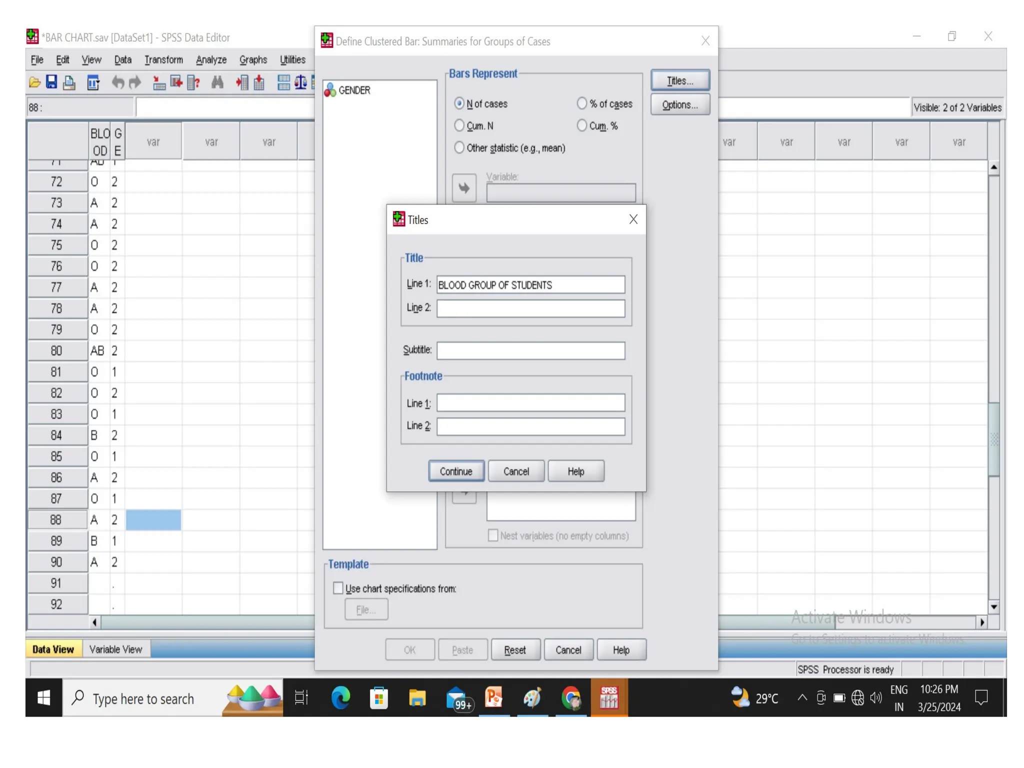
CLUSTERED BAR CHART
•Draw a clustered and stacked bar diagram for
the following data on the blood group of 90
students in a class.
O B AB B A B A
O B AB B A B A
A O AB O O A
A B A A AB O
A A O A O A
A O A O O B
O O B A B AB A
O O O B A B A
A A A A AB AB B
O B AB O B O B
A A A AB O B A
A A O O B AB B
A A AB O A B A
MALE FEMALE
PARAMETRIC TESTS ANDNON-PARAMETRIC
TESTS
• Parametric tests are statistical tests that make
assumptions about the distribution of a
population from which a sample is drawn.
• Non-parametric tests are distribution-free
tests that do not require a distribution to meet
certain assumptions
52.
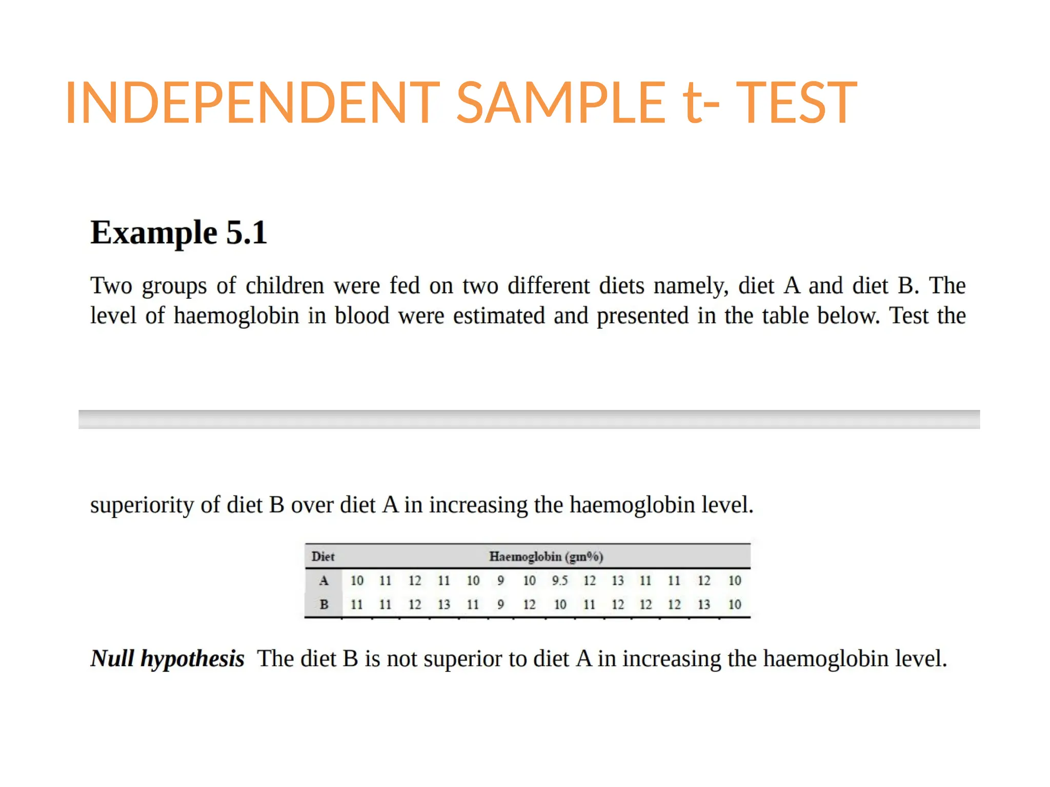
STUDENTS t-TEST
• Thet-test enables us to test the significance of
difference between two sample means or
significance of a single mean. These procedures
are called two-sample test and one sample test.
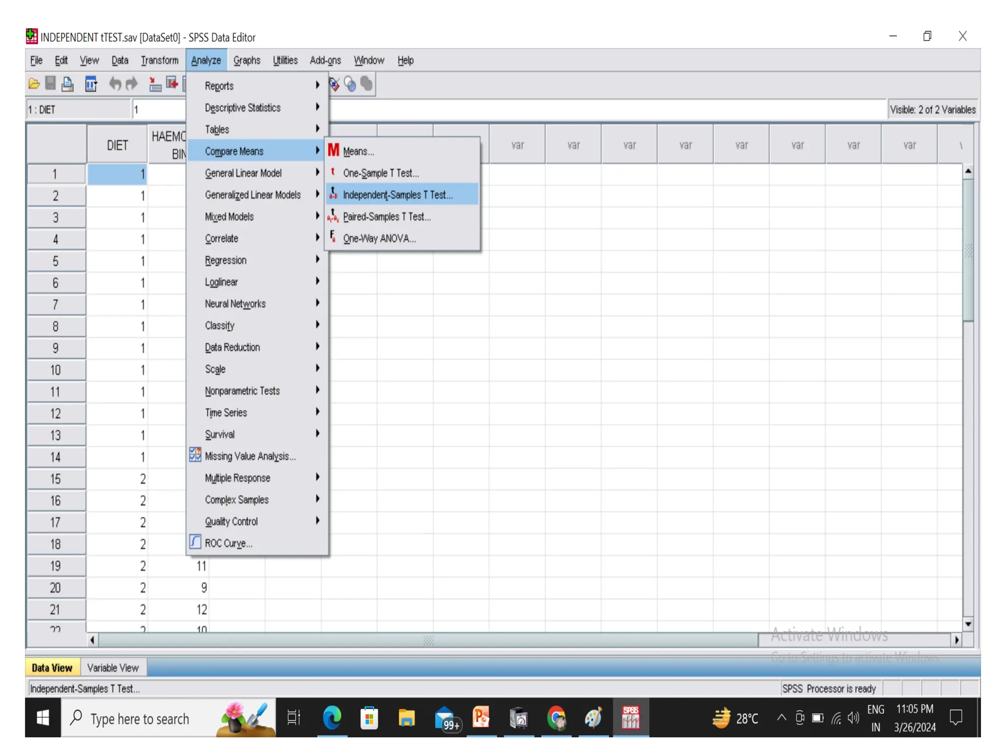
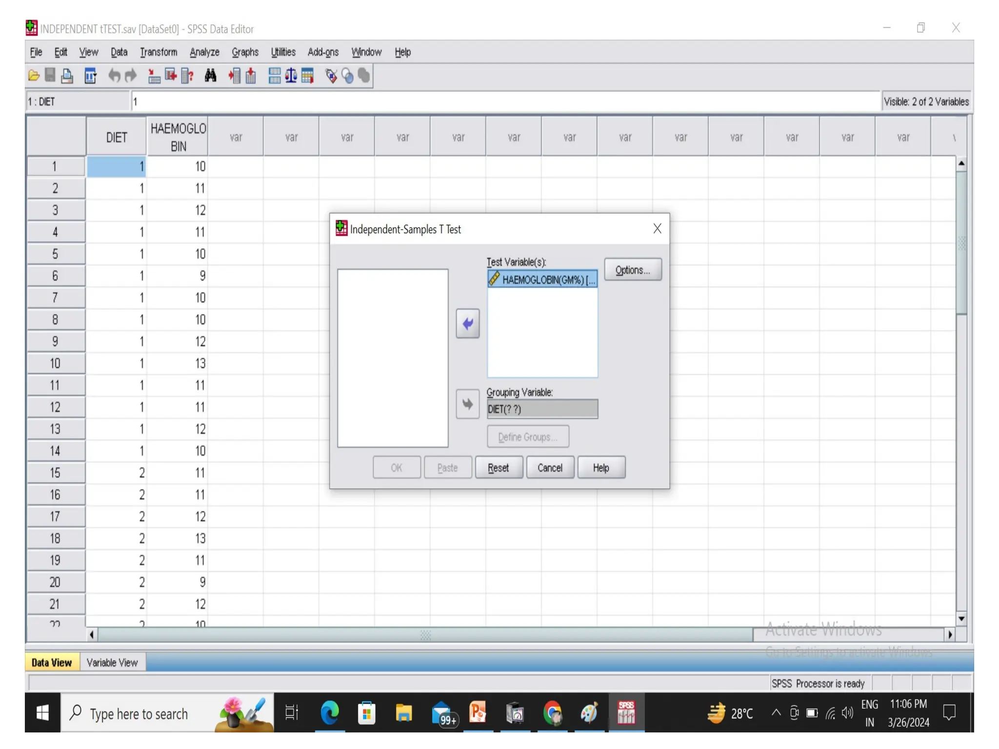
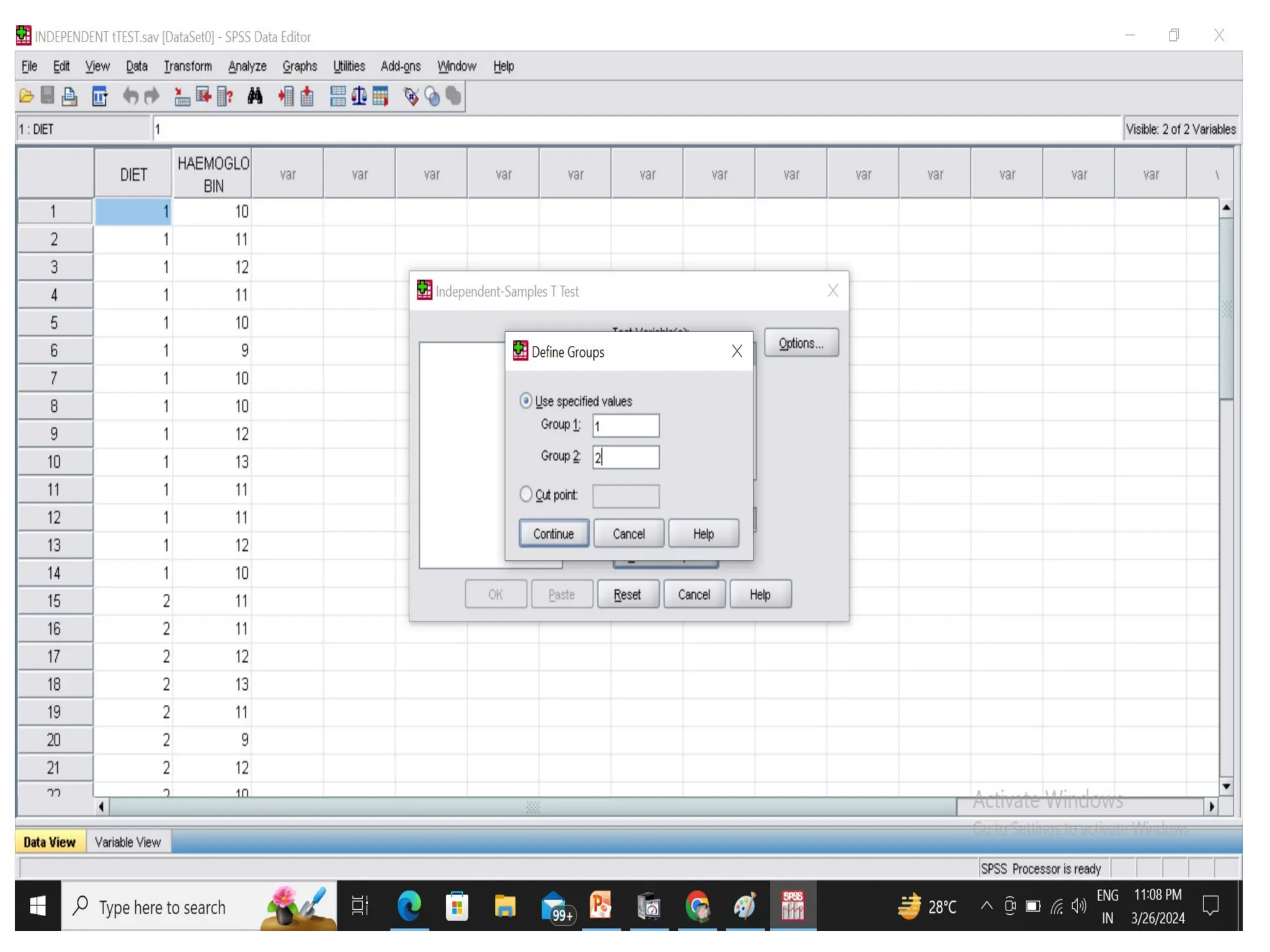
• Independent sample t-test : compares means for
two groups of cases.
Eg., A sample of 100 individuals is drawn from the
population and randomly divided into two groups
and one group is subjected to some experimental
conditions and the rest to control conditions.
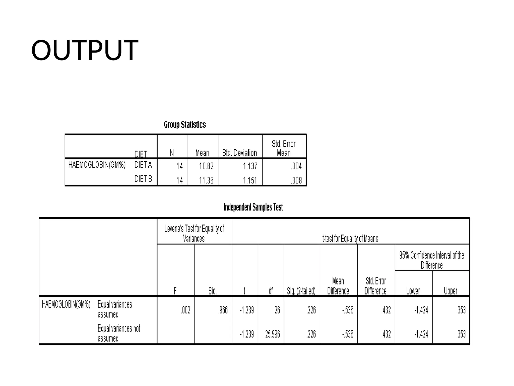
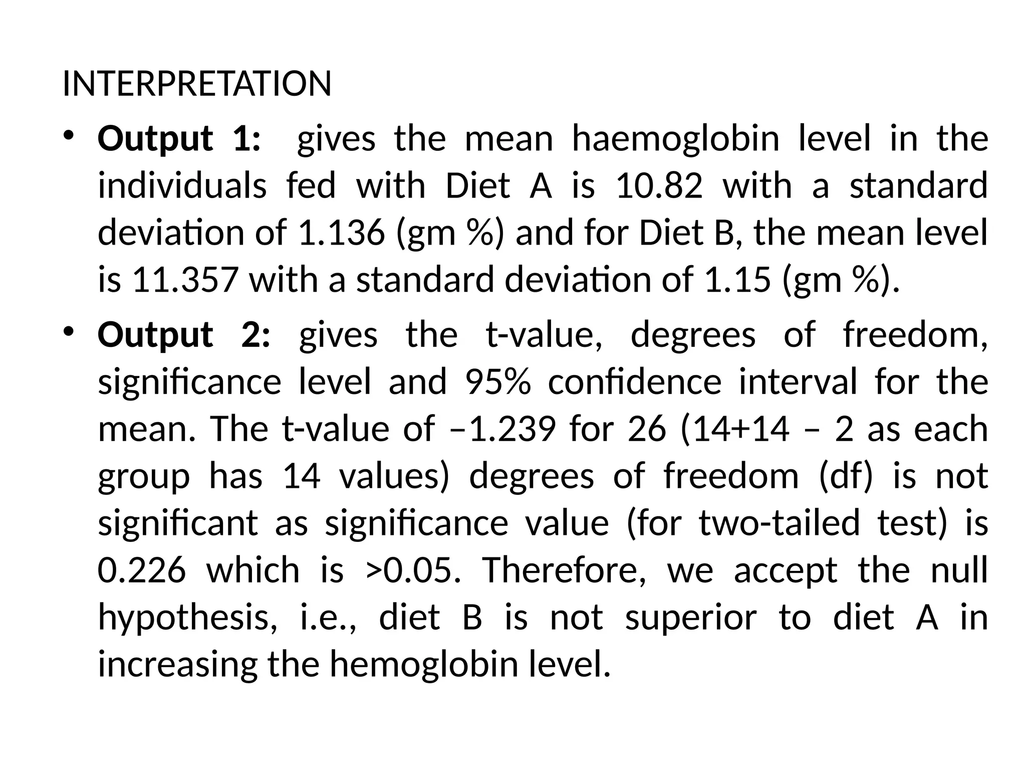
INTERPRETATION
• Output 1:gives the mean haemoglobin level in the
individuals fed with Diet A is 10.82 with a standard
deviation of 1.136 (gm %) and for Diet B, the mean level
is 11.357 with a standard deviation of 1.15 (gm %).
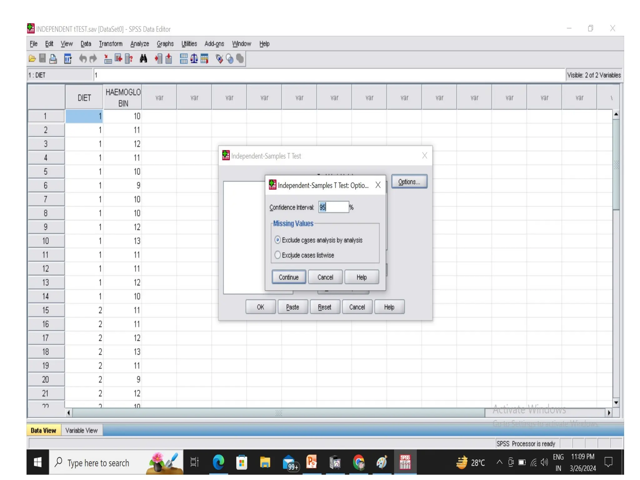
• Output 2: gives the t-value, degrees of freedom,
significance level and 95% confidence interval for the
mean. The t-value of –1.239 for 26 (14+14 – 2 as each
group has 14 values) degrees of freedom (df) is not
significant as significance value (for two-tailed test) is
0.226 which is >0.05. Therefore, we accept the null
hypothesis, i.e., diet B is not superior to diet A in
increasing the hemoglobin level.
62.
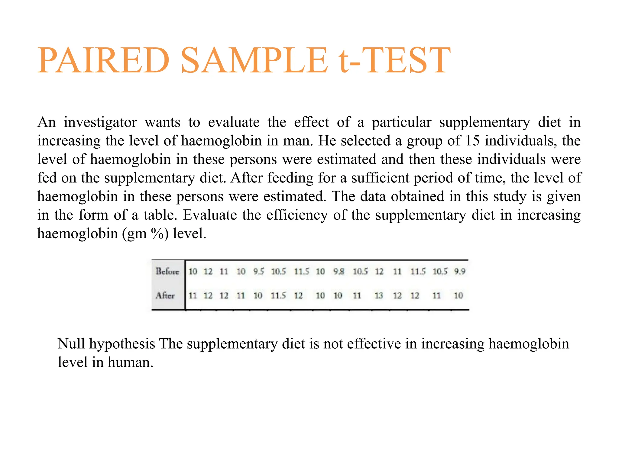
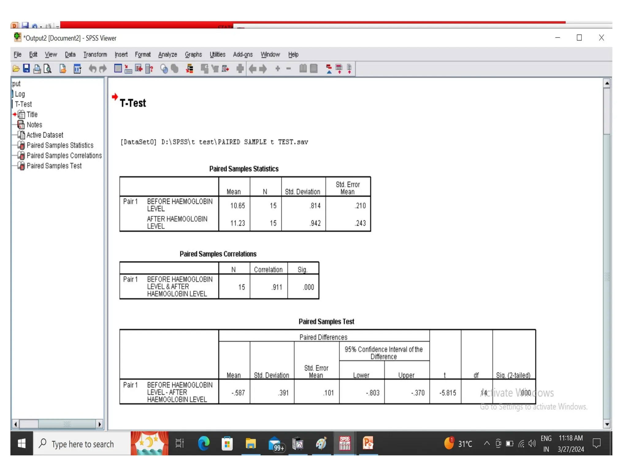
PAIRED SAMPLE t-TEST
Aninvestigator wants to evaluate the effect of a particular supplementary diet in
increasing the level of haemoglobin in man. He selected a group of 15 individuals, the
level of haemoglobin in these persons were estimated and then these individuals were
fed on the supplementary diet. After feeding for a sufficient period of time, the level of
haemoglobin in these persons were estimated. The data obtained in this study is given
in the form of a table. Evaluate the efficiency of the supplementary diet in increasing
haemoglobin (gm %) level.
Null hypothesis The supplementary diet is not effective in increasing haemoglobin
level in human.
66.
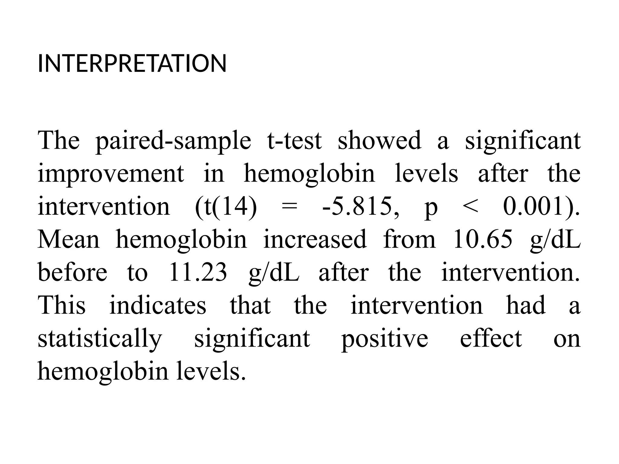
INTERPRETATION
The paired-sample t-testshowed a significant
improvement in hemoglobin levels after the
intervention (t(14) = -5.815, p < 0.001).
Mean hemoglobin increased from 10.65 g/dL
before to 11.23 g/dL after the intervention.
This indicates that the intervention had a
statistically significant positive effect on
hemoglobin levels.