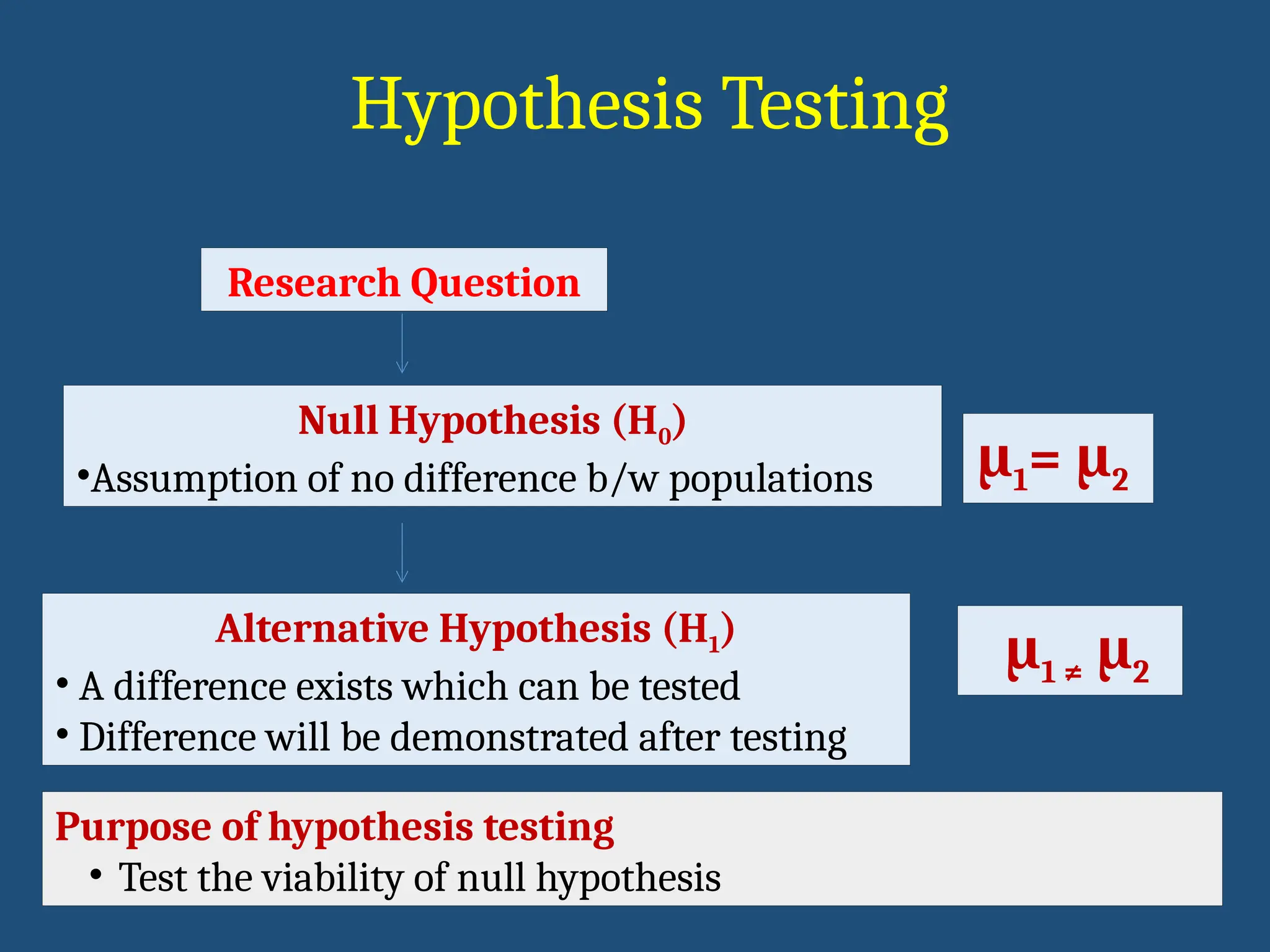
Hypothesis Testing
Research Question
NullHypothesis (H0)
•Assumption of no difference b/w populations
Alternative Hypothesis (H1)
• A difference exists which can be tested
• Difference will be demonstrated after testing
Purpose of hypothesis testing
• Test the viability of null hypothesis
μ1= μ2
μ1 ≠ μ2
4.
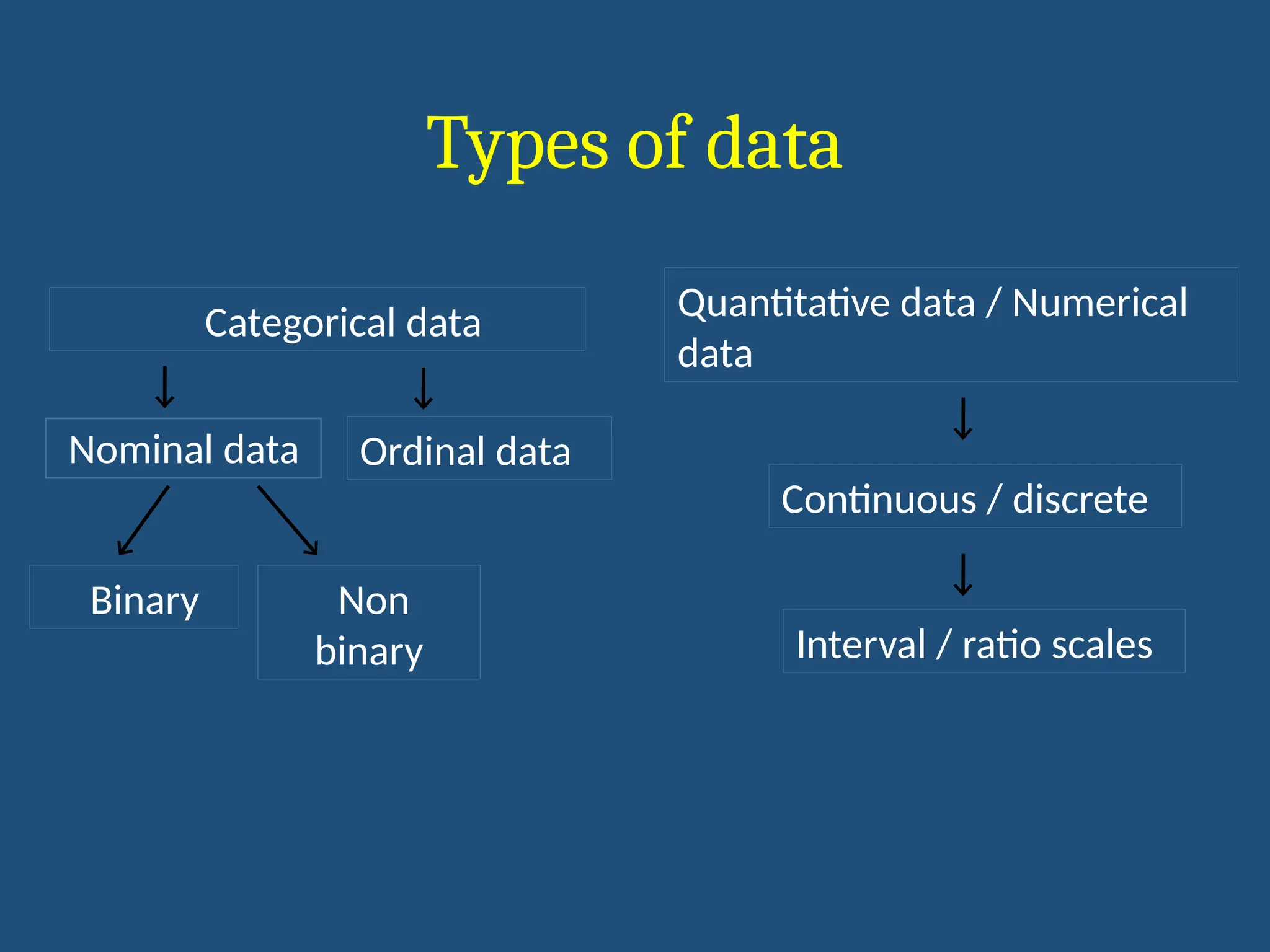
Types of data
Ordinaldata
Non
binary
Nominal data
Binary
Quantitative data / Numerical
data
Continuous / discrete
Interval / ratio scales
Categorical data
5.
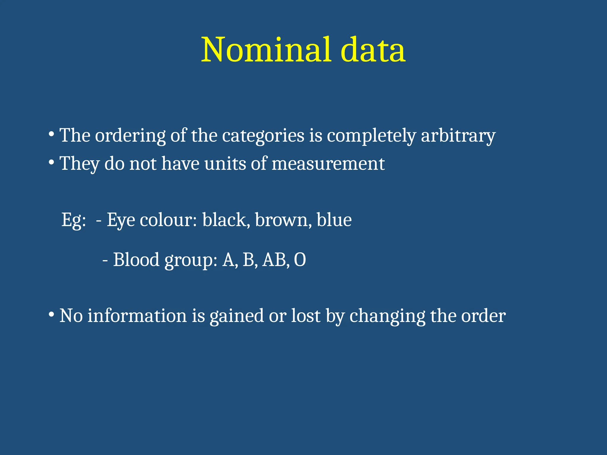
Nominal data
• Theordering of the categories is completely arbitrary
• They do not have units of measurement
Eg: - Eye colour: black, brown, blue
- Blood group: A, B, AB, O
• No information is gained or lost by changing the order
6.
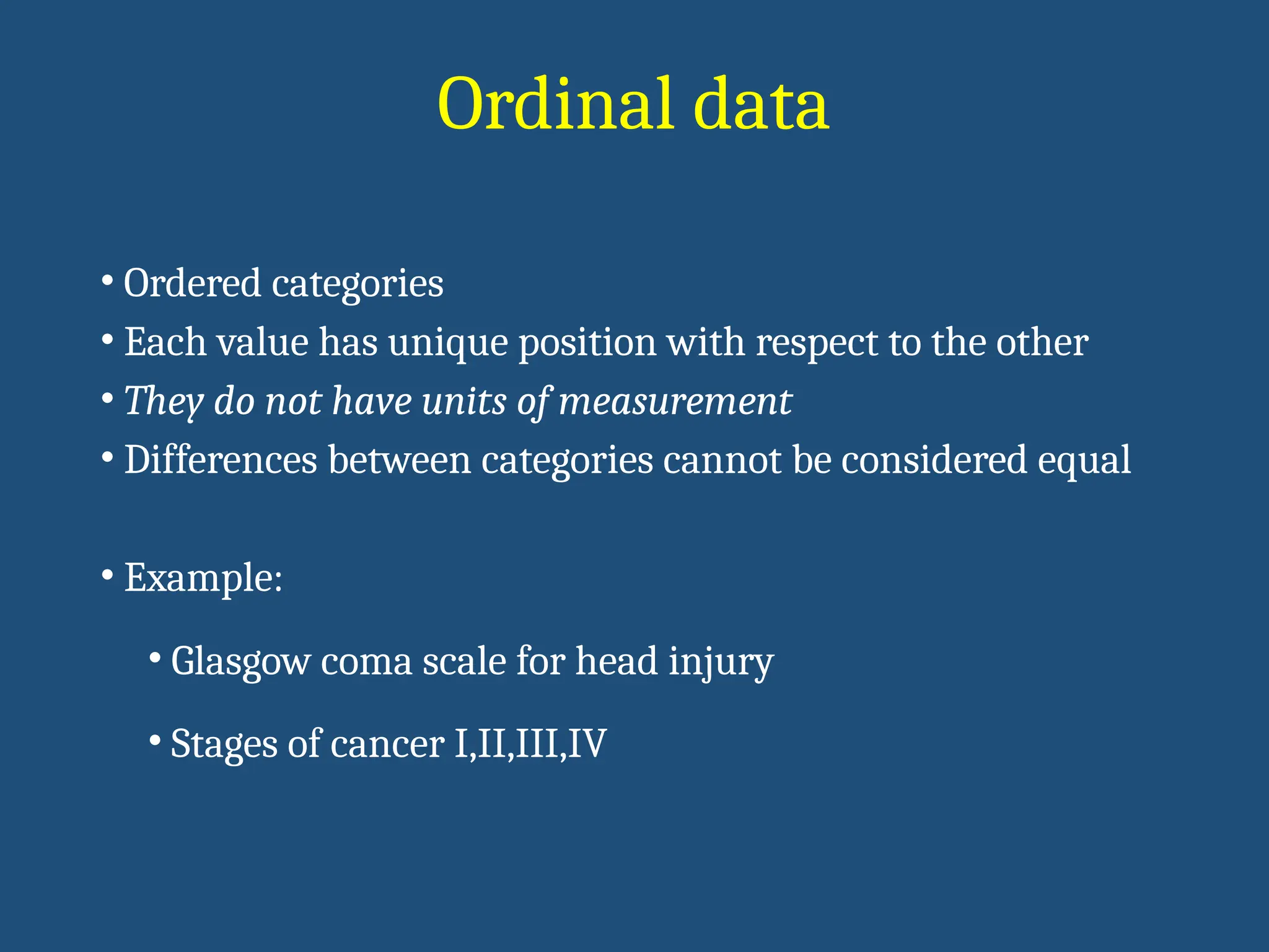
Ordinal data
• Orderedcategories
• Each value has unique position with respect to the other
• They do not have units of measurement
• Differences between categories cannot be considered equal
• Example:
• Glasgow coma scale for head injury
• Stages of cancer I,II,III,IV
7.
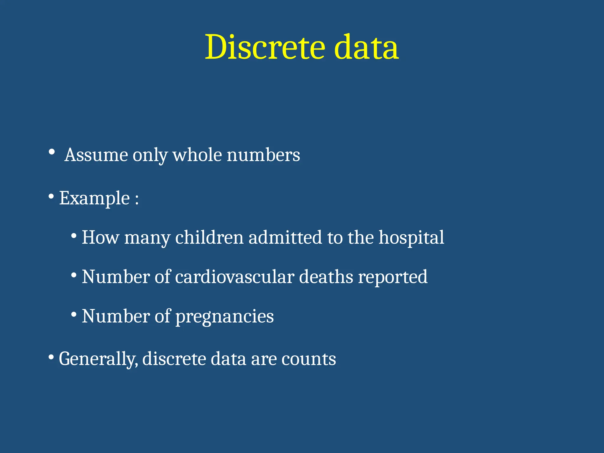
Discrete data
• Assumeonly whole numbers
• Example :
• How many children admitted to the hospital
• Number of cardiovascular deaths reported
• Number of pregnancies
• Generally, discrete data are counts
8.
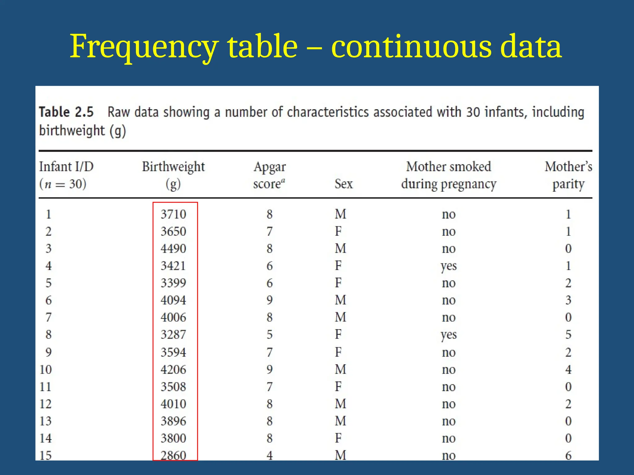
Continuous data
• Valuesthat are fractions or decimals
• Values between variables depends on the instrument used
• Examples :
• Cholesterol level (μg/ml)
• BP ( mm Hg)
• BMI (kg/m2)
• Generally, continuous data come from measurements
9.
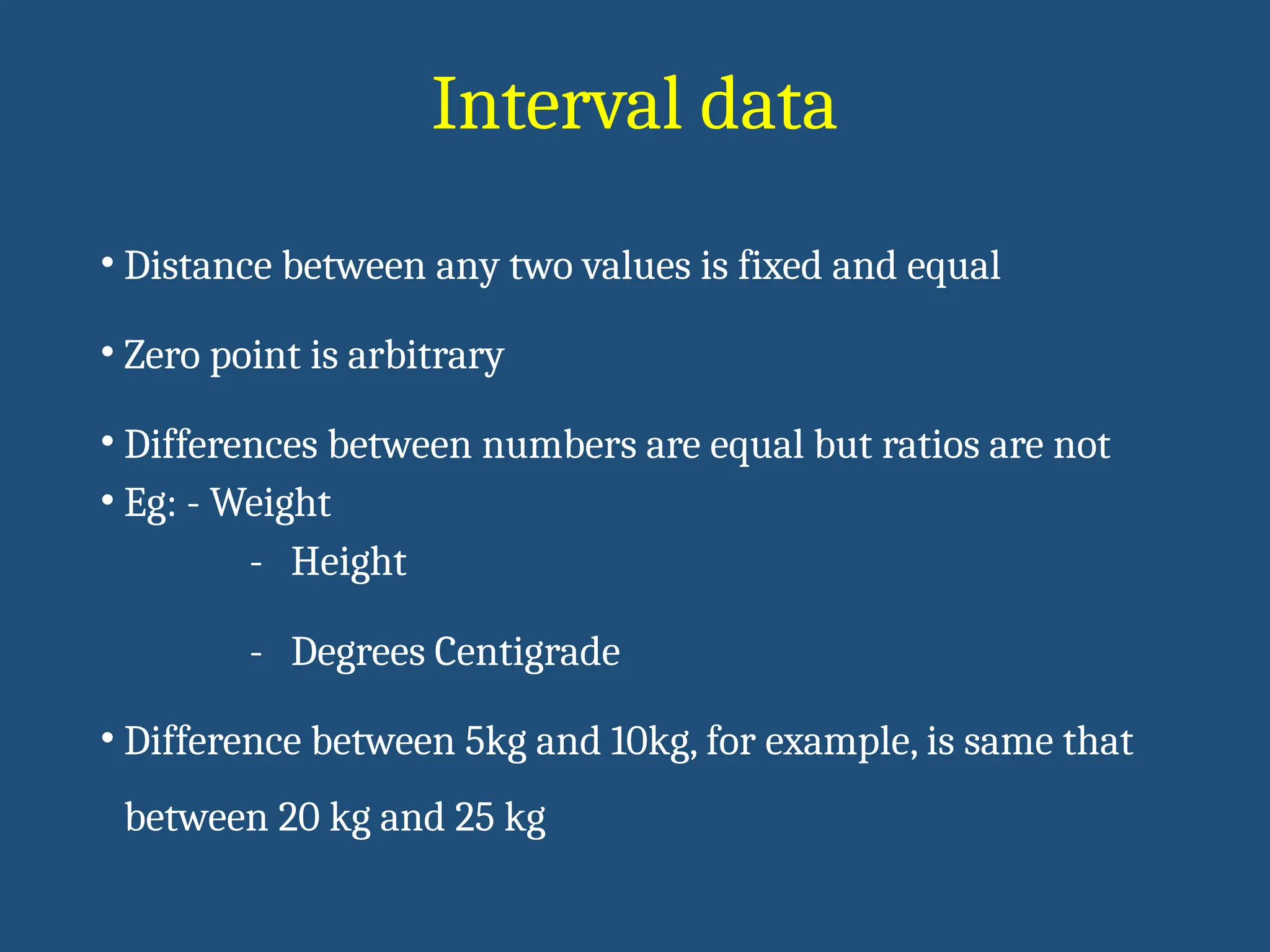
Interval data
• Distancebetween any two values is fixed and equal
• Zero point is arbitrary
• Differences between numbers are equal but ratios are not
• Eg: - Weight
- Height
- Degrees Centigrade
• Difference between 5kg and 10kg, for example, is same that
between 20 kg and 25 kg
10.
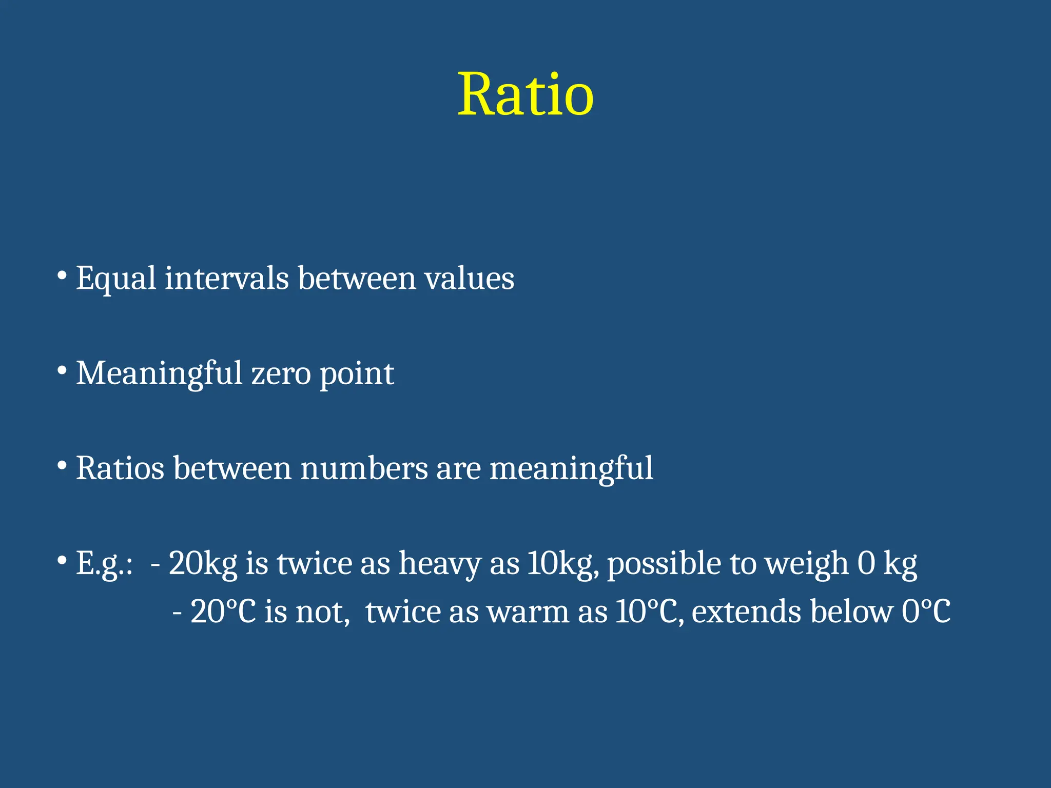
Ratio
• Equal intervalsbetween values
• Meaningful zero point
• Ratios between numbers are meaningful
• E.g.: - 20kg is twice as heavy as 10kg, possible to weigh 0 kg
- 20°C is not, twice as warm as 10°C, extends below 0°C
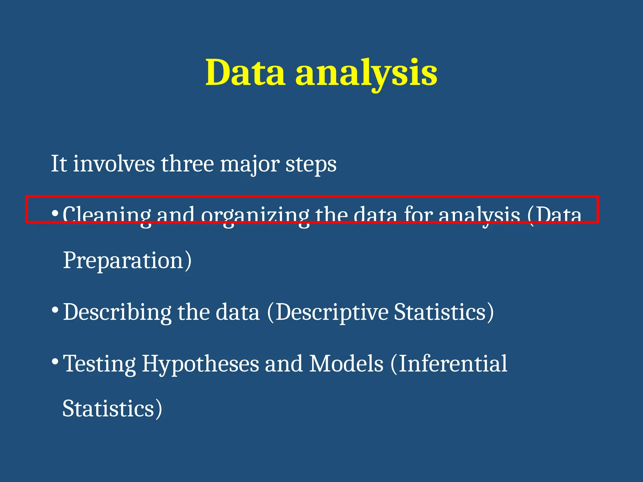
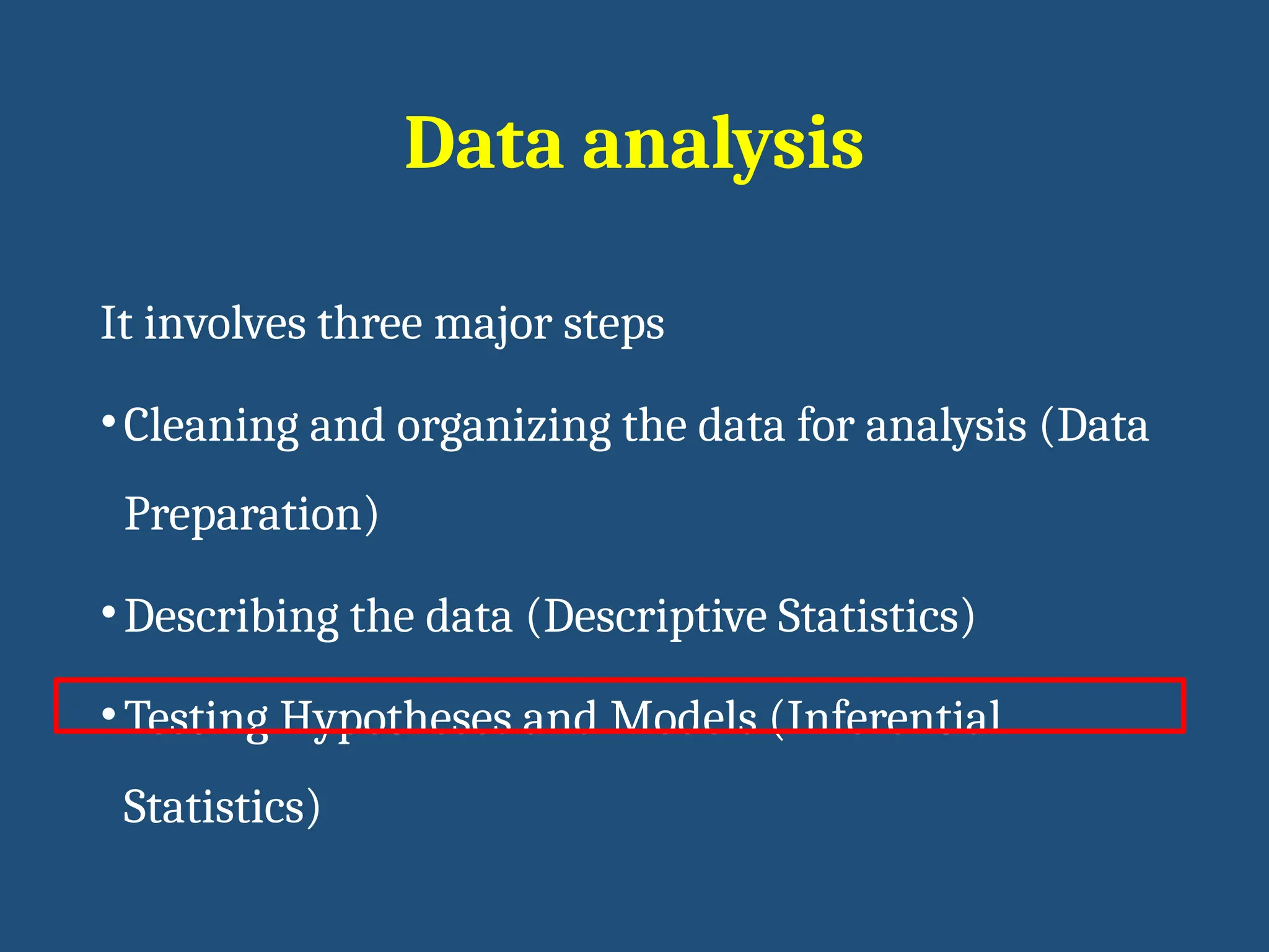
Data analysis
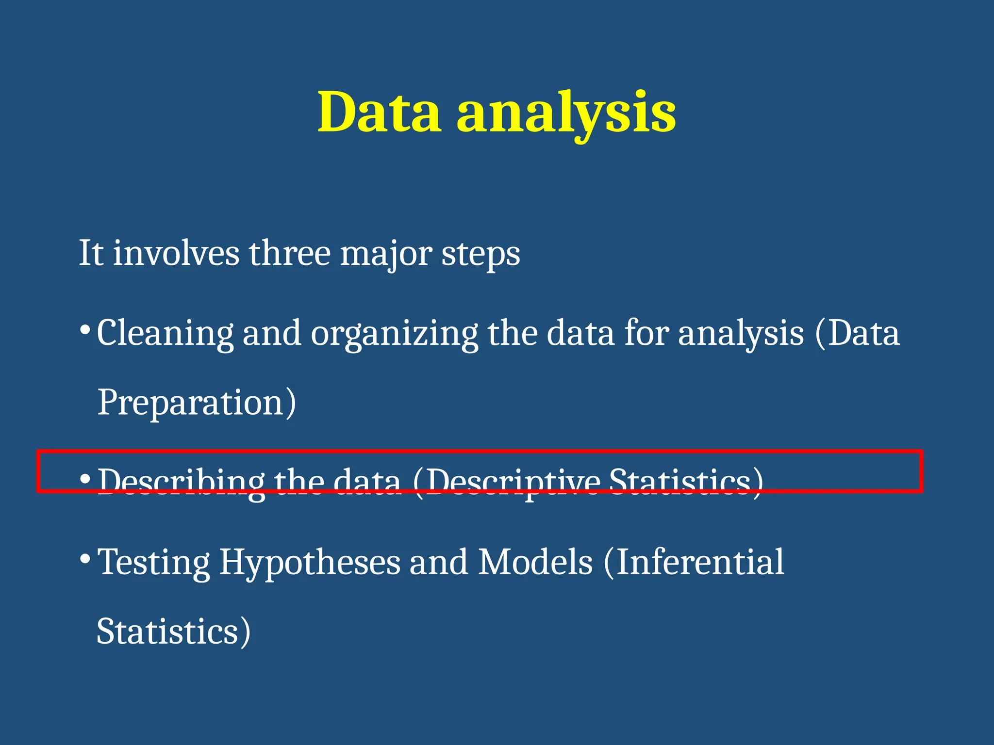
It involvesthree major steps
•Cleaning and organizing the data for analysis (Data
Preparation)
•Describing the data (Descriptive Statistics)
•Testing Hypotheses and Models (Inferential
Statistics)
13.
Data analysis
It involvesthree major steps
•Cleaning and organizing the data for analysis (Data
Preparation)
•Describing the data (Descriptive Statistics)
•Testing Hypotheses and Models (Inferential
Statistics)
14.
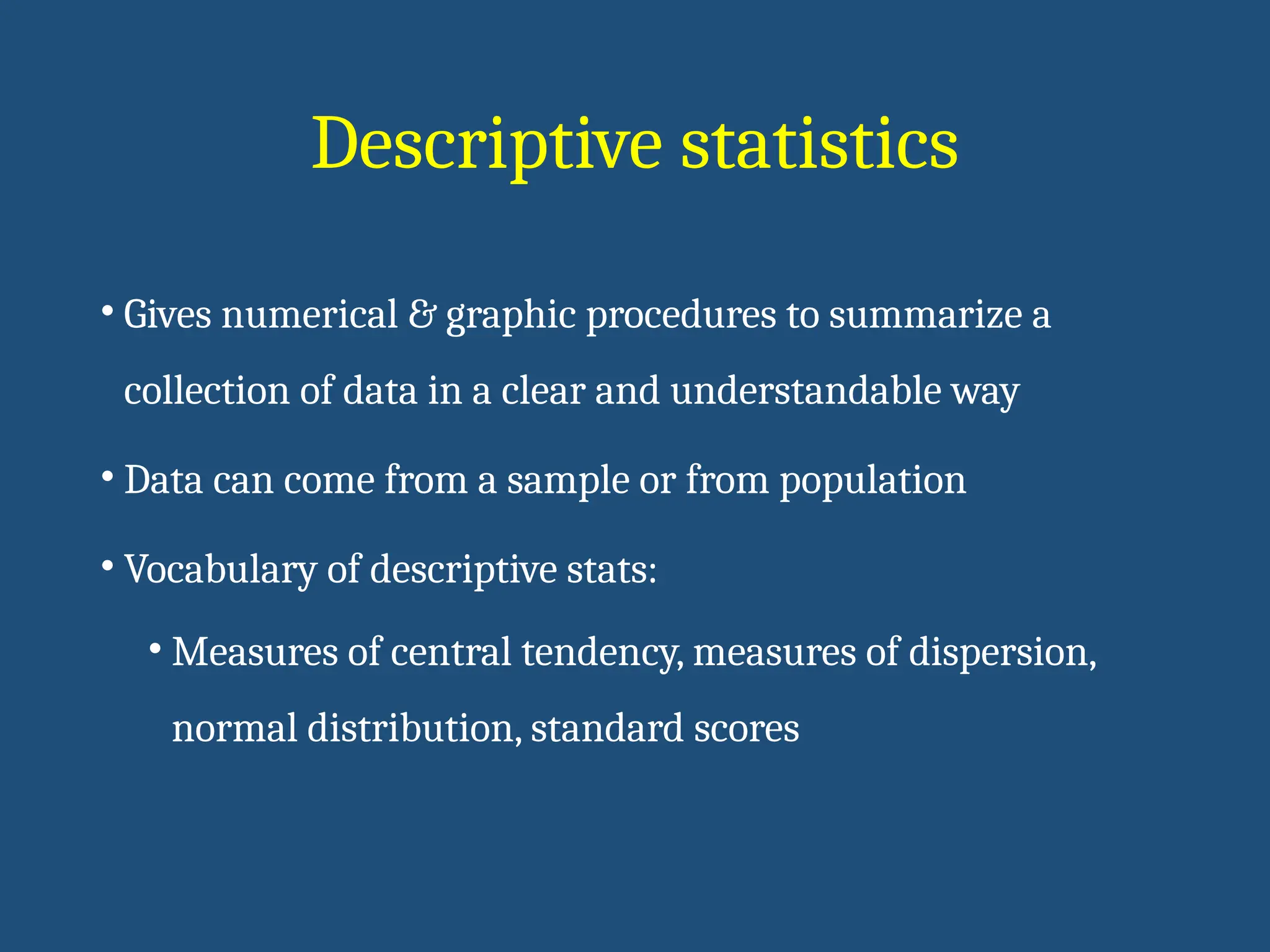
Descriptive statistics
• Givesnumerical & graphic procedures to summarize a
collection of data in a clear and understandable way
• Data can come from a sample or from population
• Vocabulary of descriptive stats:
• Measures of central tendency, measures of dispersion,
normal distribution, standard scores
15.
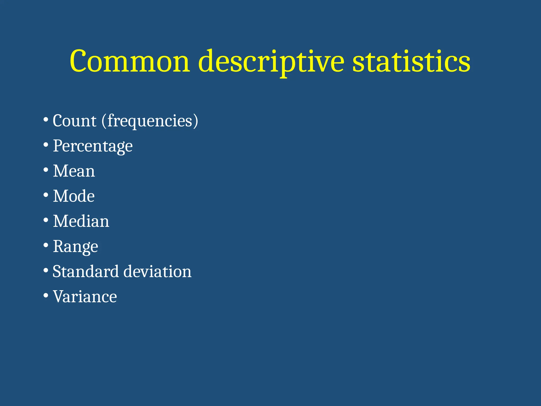
Common descriptive statistics
•Count (frequencies)
• Percentage
• Mean
• Mode
• Median
• Range
• Standard deviation
• Variance
16.
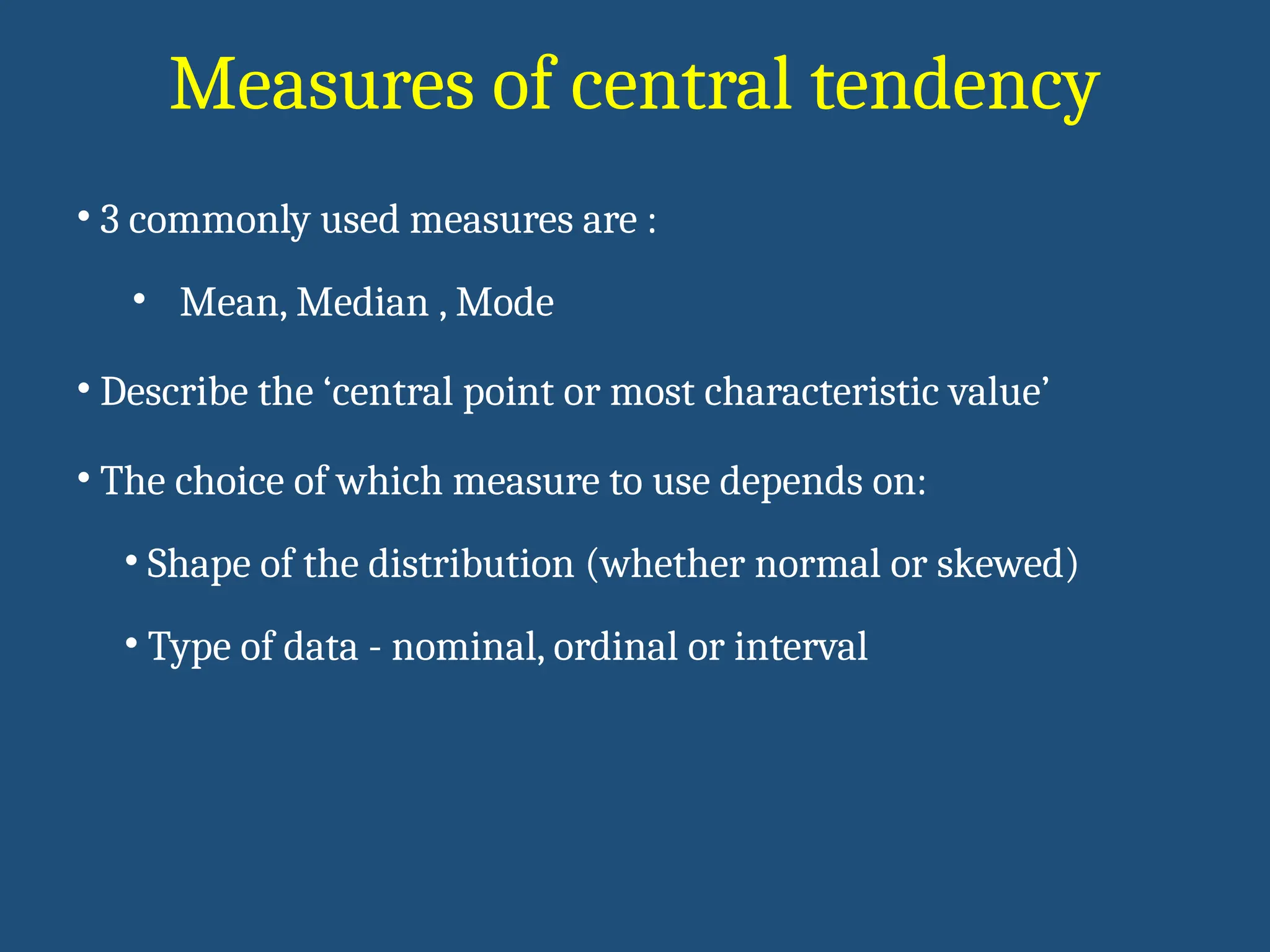
Measures of centraltendency
• 3 commonly used measures are :
• Mean, Median , Mode
• Describe the ‘central point or most characteristic value’
• The choice of which measure to use depends on:
• Shape of the distribution (whether normal or skewed)
• Type of data - nominal, ordinal or interval
17.
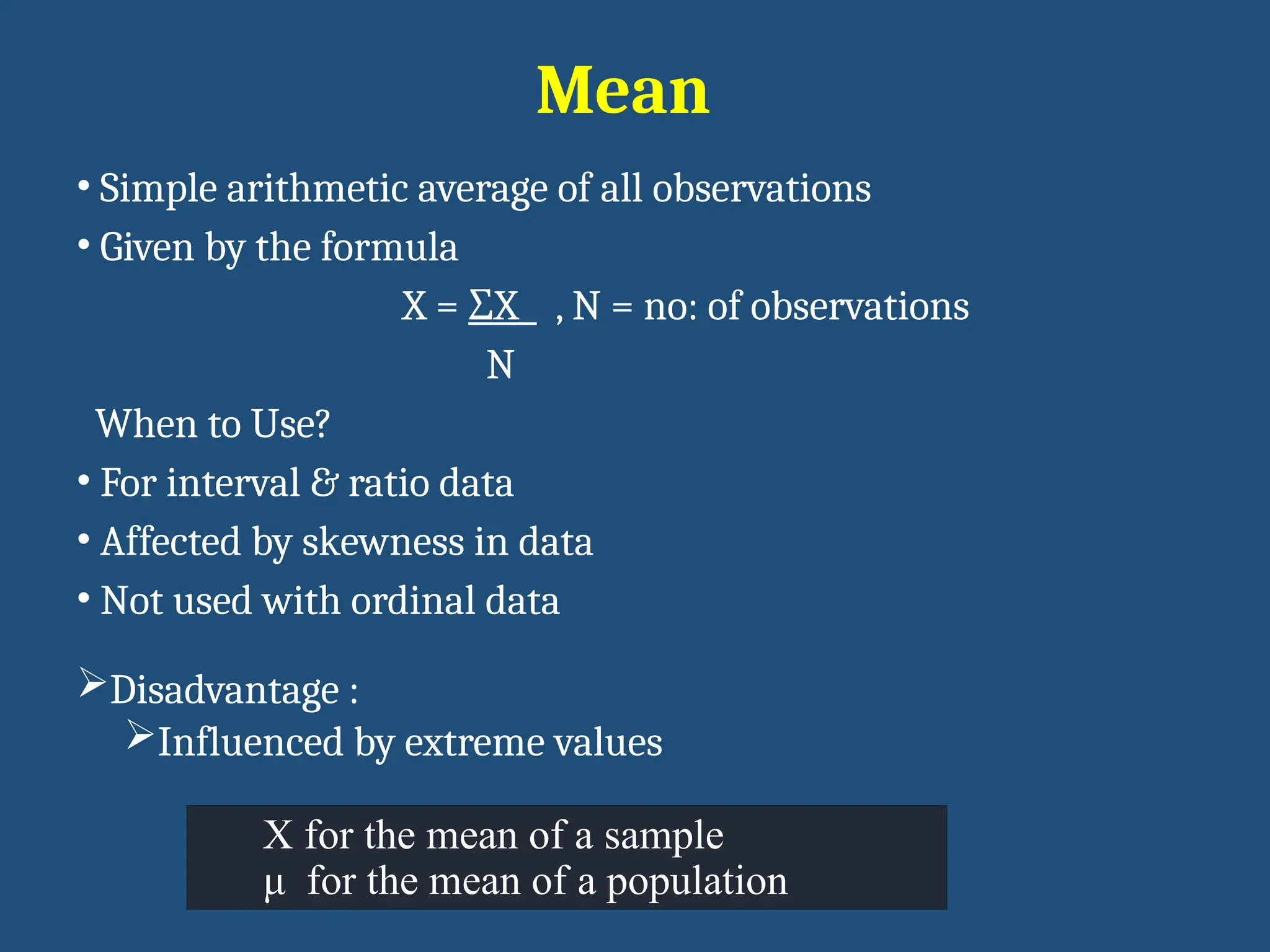
Mean
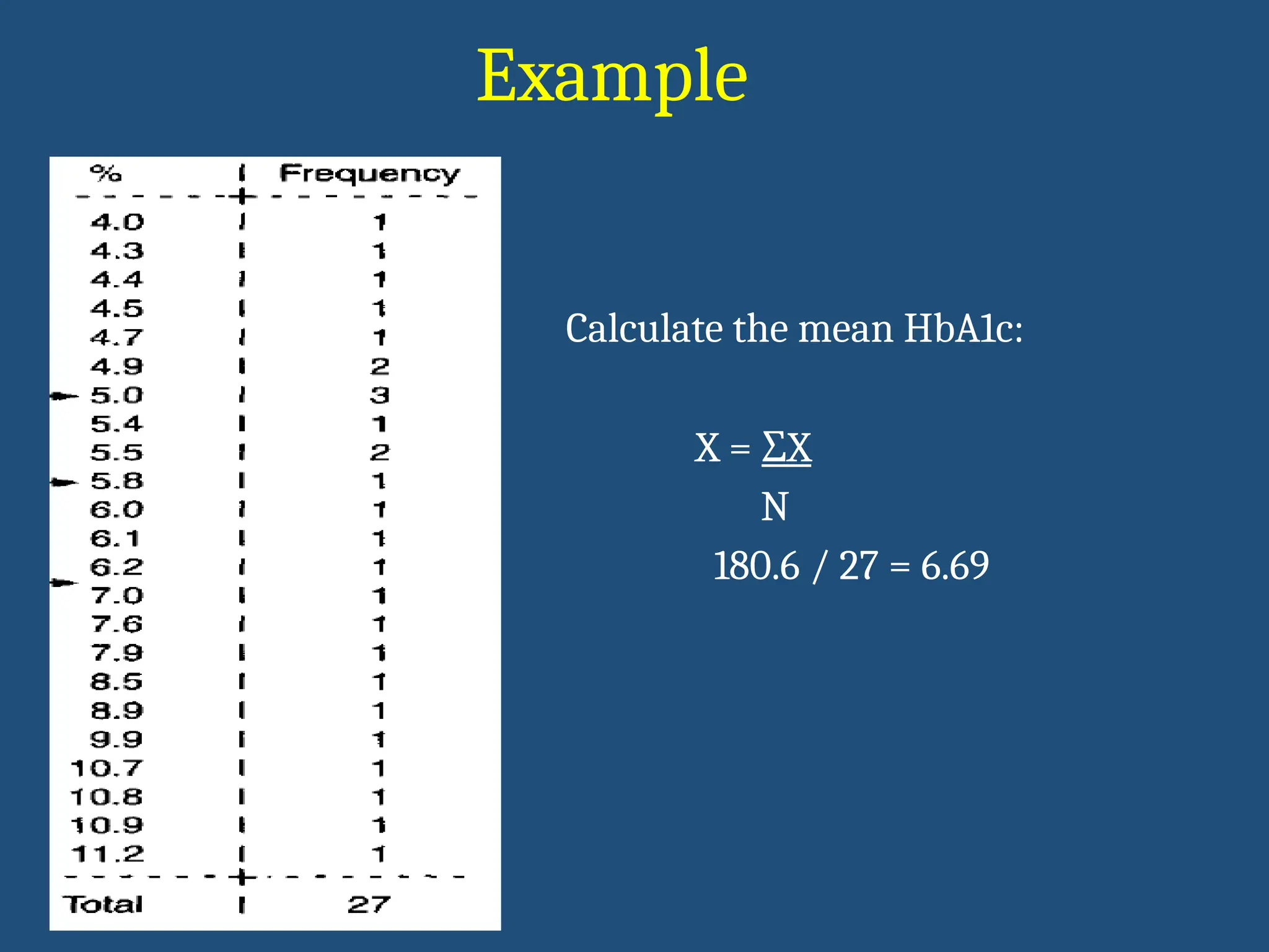
• Simple arithmeticaverage of all observations
• Given by the formula
X = ΣX , N = no: of observations
N
When to Use?
• For interval & ratio data
• Affected by skewness in data
• Not used with ordinal data
Disadvantage :
Influenced by extreme values
X for the mean of a sample
μ for the mean of a population
Median
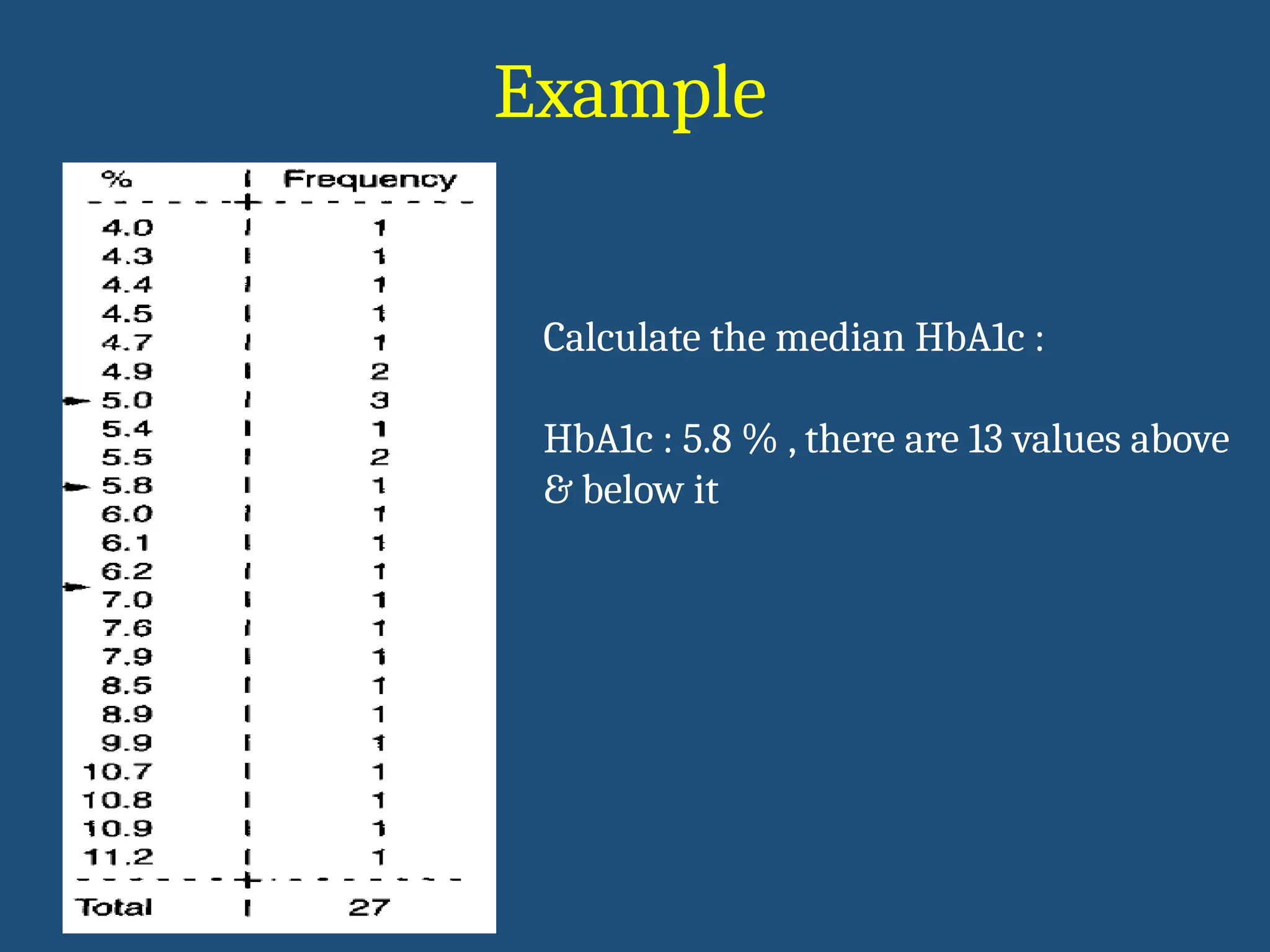
• Median isthe middle value, if data are arranged in ↑ order.
• Odd no.: middle value
• Even no.: mean of 2 middle observations
- Presence of outliers
- Data are measured in ordinal scale
Eg.: SES – low, middle, upper
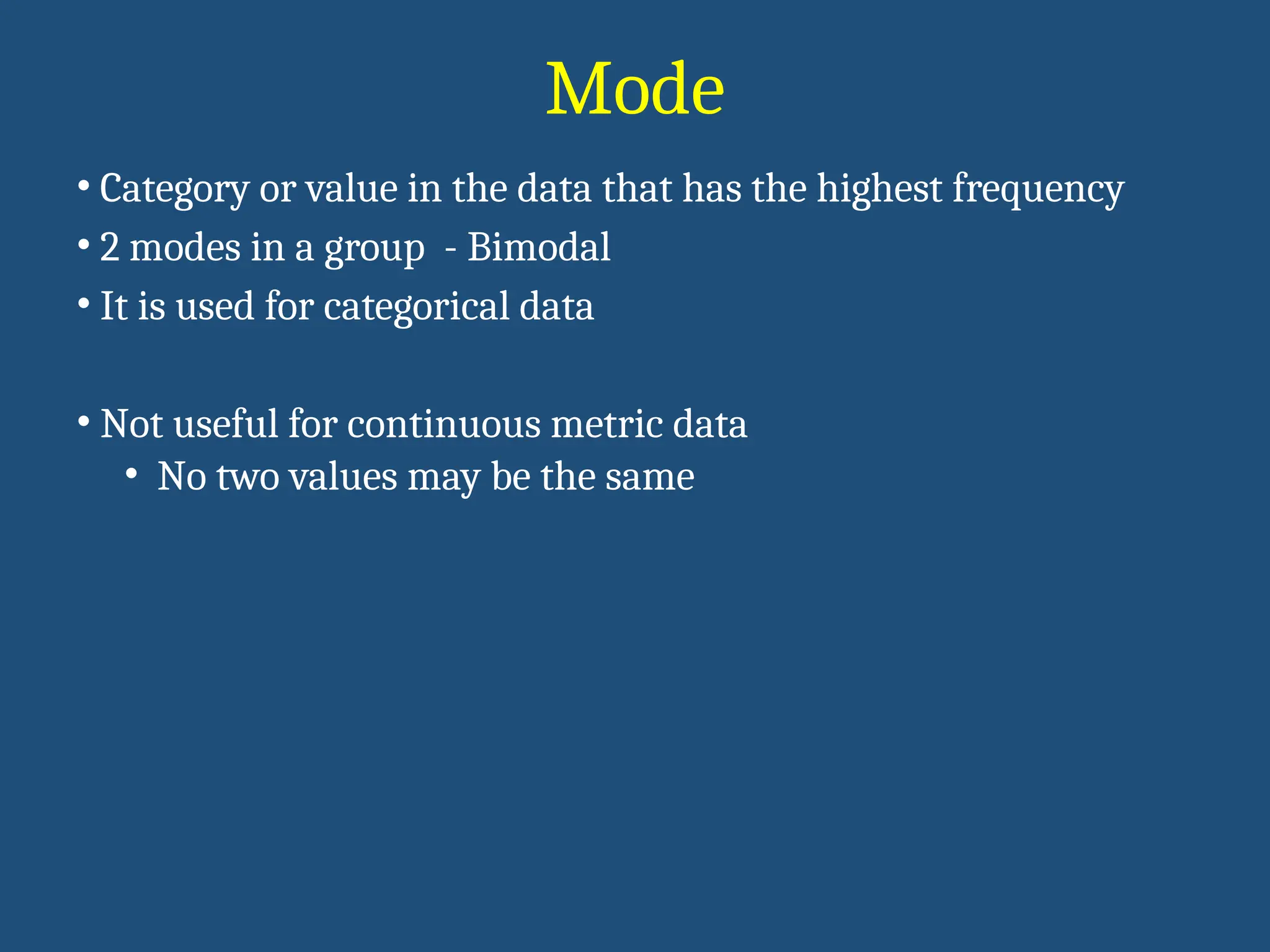
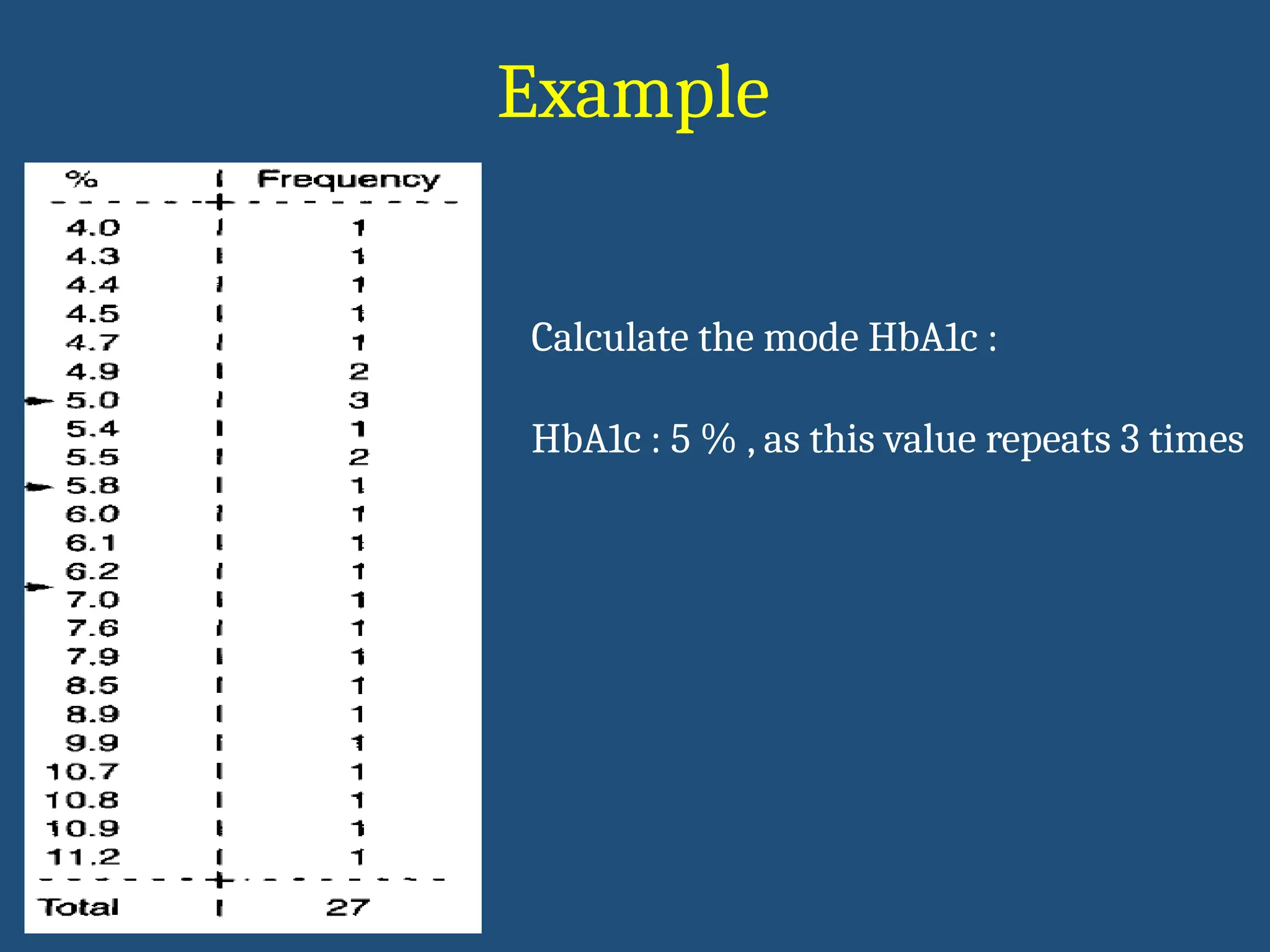
Mode
• Category orvalue in the data that has the highest frequency
• 2 modes in a group - Bimodal
• It is used for categorical data
• Not useful for continuous metric data
• No two values may be the same
Measure of centraltendency
Type of variable Mode Median Mean
Nominal Yes No No
Ordinal Yes Yes Yes
Metric data Yes Yes, if
distribution is
skewed
Yes
Metric continuous No Yes, if
distribution is
skewed
yes
24.
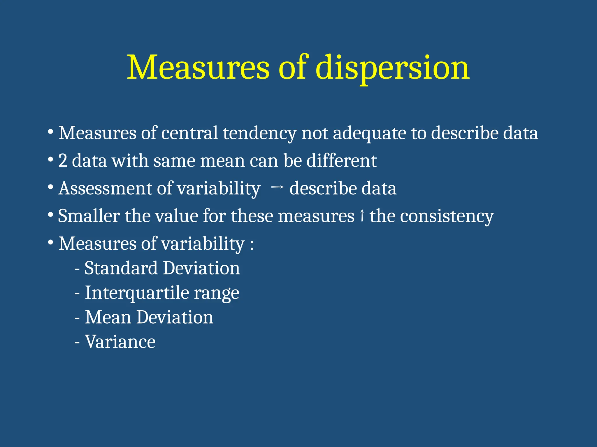
Measures of dispersion
•Measures of central tendency not adequate to describe data
• 2 data with same mean can be different
• Assessment of variability → describe data
• Smaller the value for these measures ↑ the consistency
• Measures of variability :
- Standard Deviation
- Interquartile range
- Mean Deviation
- Variance
25.
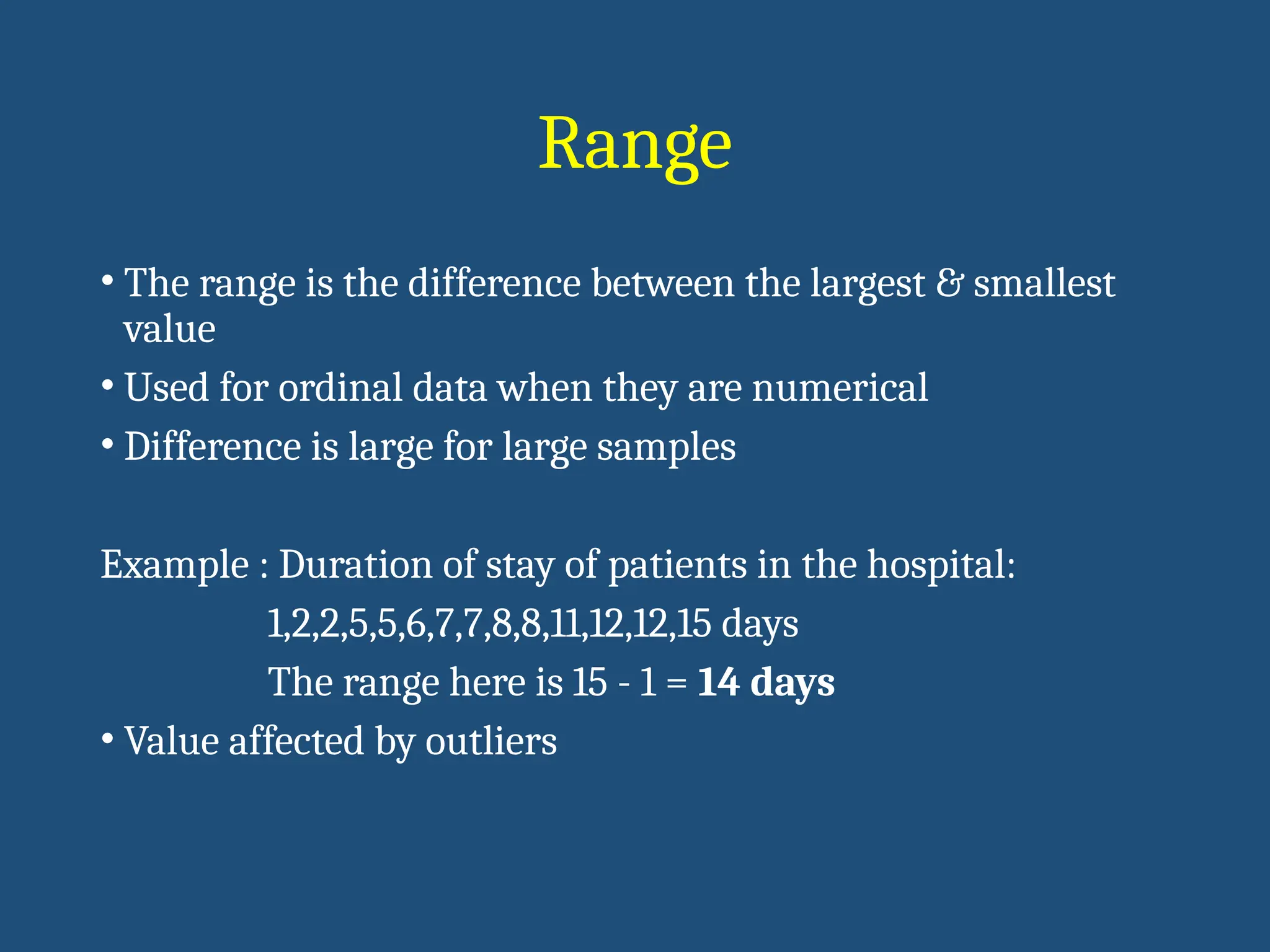
Range
• The rangeis the difference between the largest & smallest
value
• Used for ordinal data when they are numerical
• Difference is large for large samples
Example : Duration of stay of patients in the hospital:
1,2,2,5,5,6,7,7,8,8,11,12,12,15 days
The range here is 15 - 1 = 14 days
• Value affected by outliers
26.
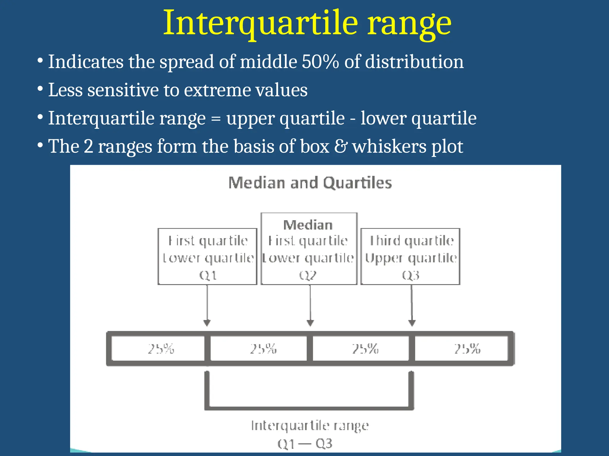
Interquartile range
• Indicatesthe spread of middle 50% of distribution
• Less sensitive to extreme values
• Interquartile range = upper quartile - lower quartile
• The 2 ranges form the basis of box & whiskers plot
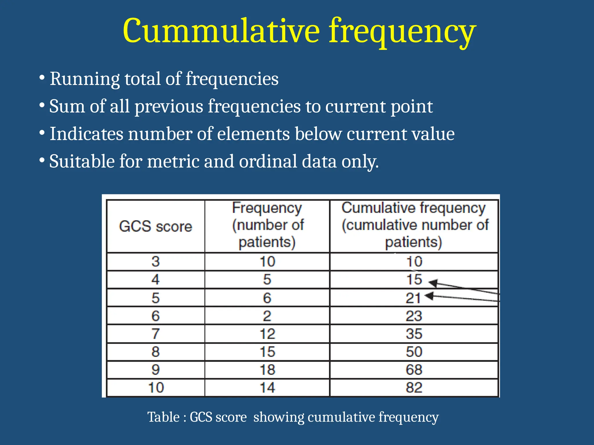
Cummulative frequency
• Runningtotal of frequencies
• Sum of all previous frequencies to current point
• Indicates number of elements below current value
• Suitable for metric and ordinal data only.
Table : GCS score showing cumulative frequency
35.
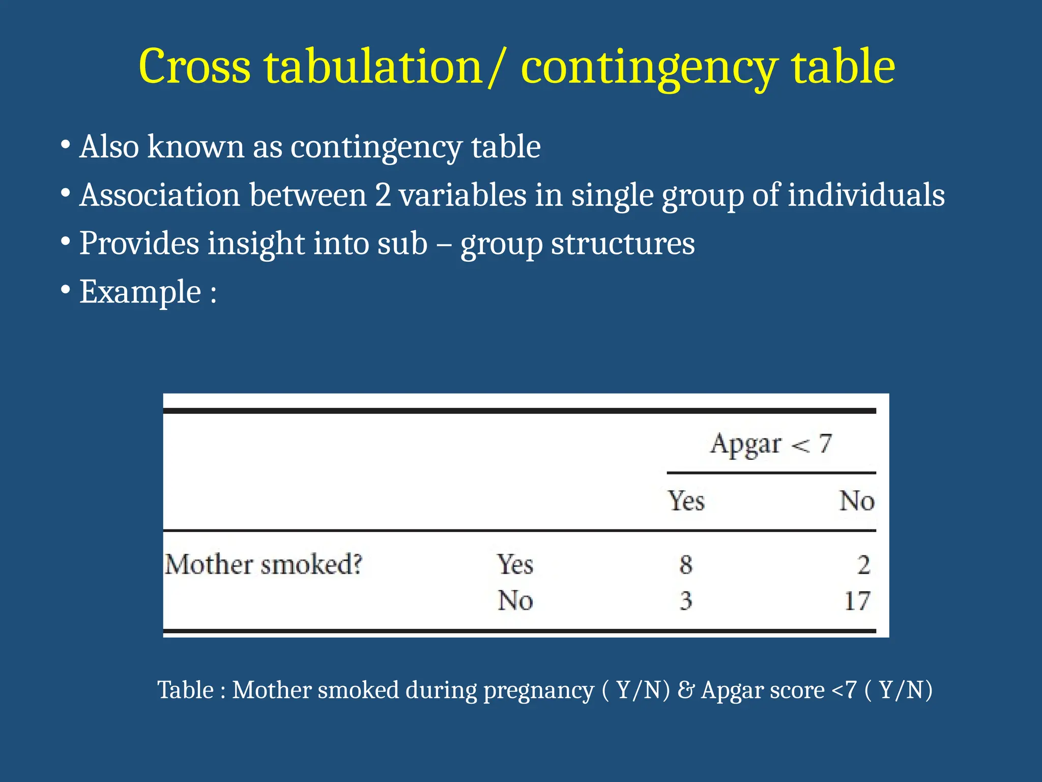
Cross tabulation/ contingencytable
• Also known as contingency table
• Association between 2 variables in single group of individuals
• Provides insight into sub – group structures
• Example :
Table : Mother smoked during pregnancy ( Y/N) & Apgar score <7 ( Y/N)
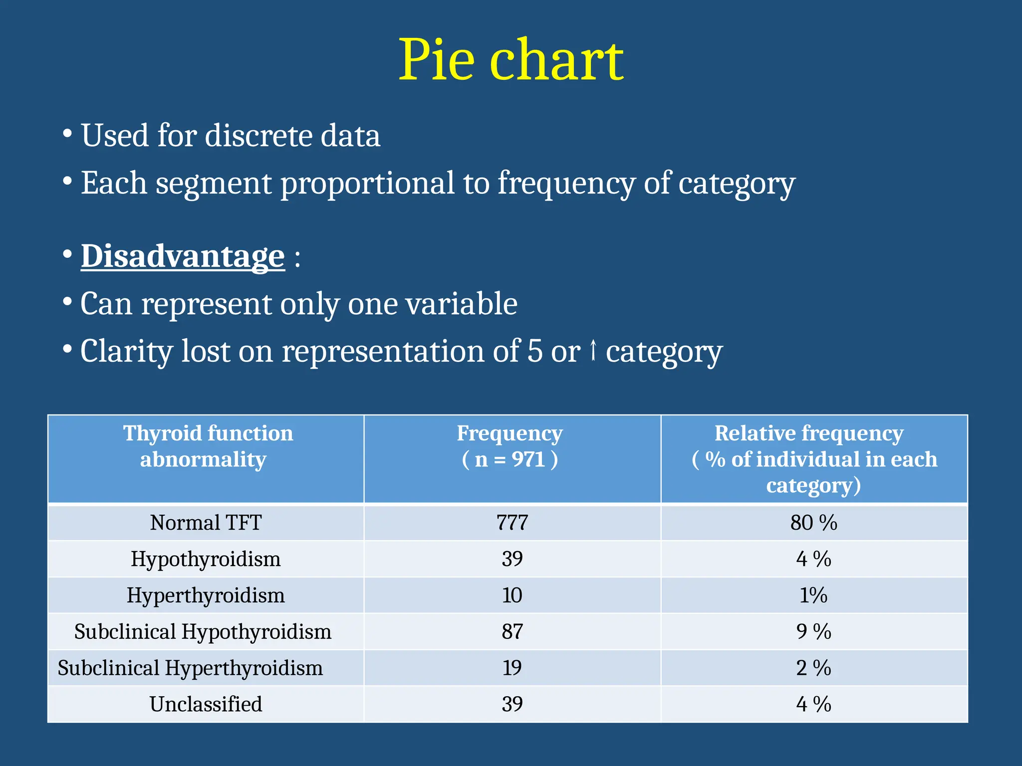
Pie chart
• Usedfor discrete data
• Each segment proportional to frequency of category
• Disadvantage :
• Can represent only one variable
• Clarity lost on representation of 5 or ↑ category
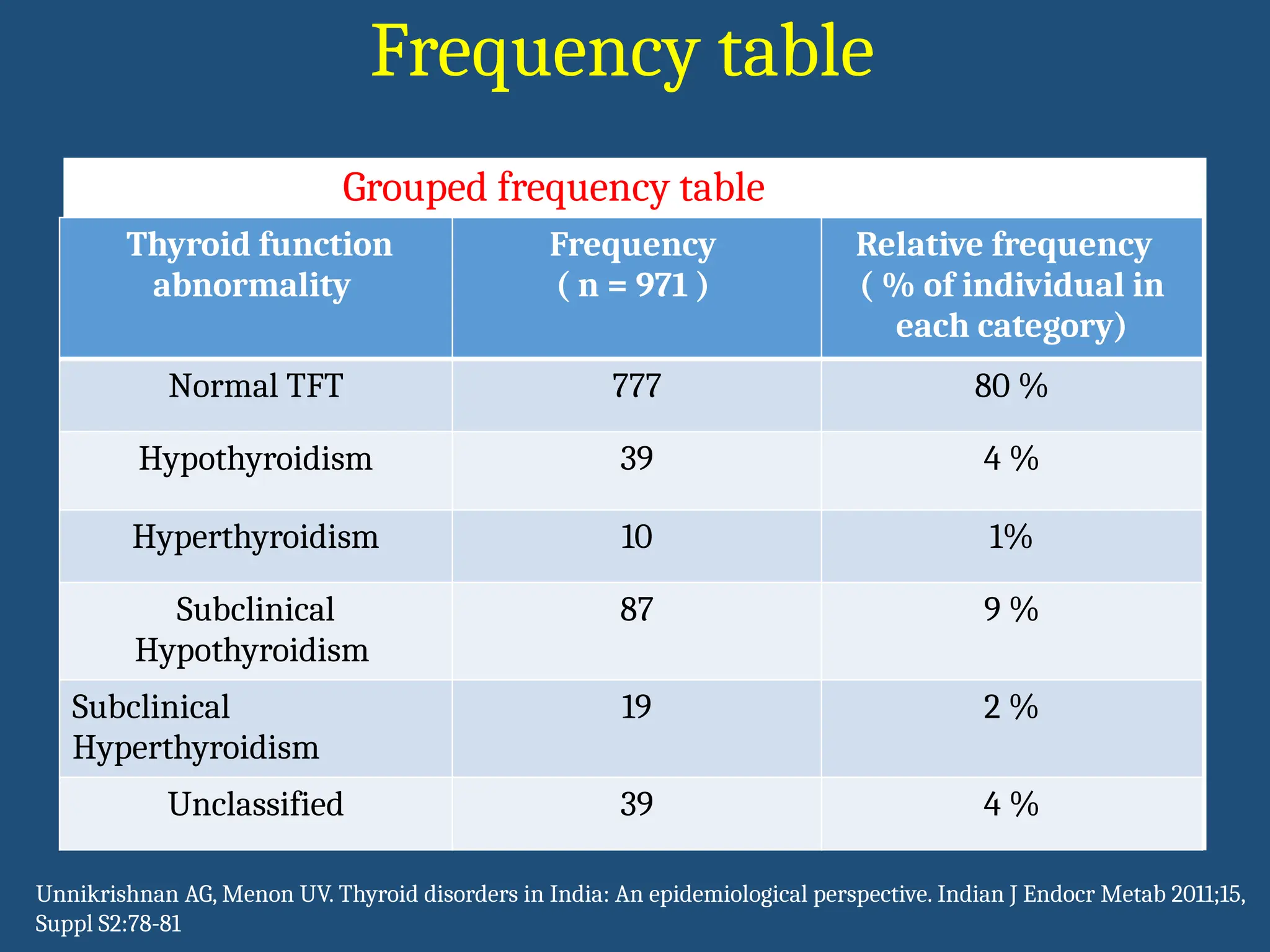
Thyroid function
abnormality
Frequency
( n = 971 )
Relative frequency
( % of individual in each
category)
Normal TFT 777 80 %
Hypothyroidism 39 4 %
Hyperthyroidism 10 1%
Subclinical Hypothyroidism 87 9 %
Subclinical Hyperthyroidism 19 2 %
Unclassified 39 4 %
38.
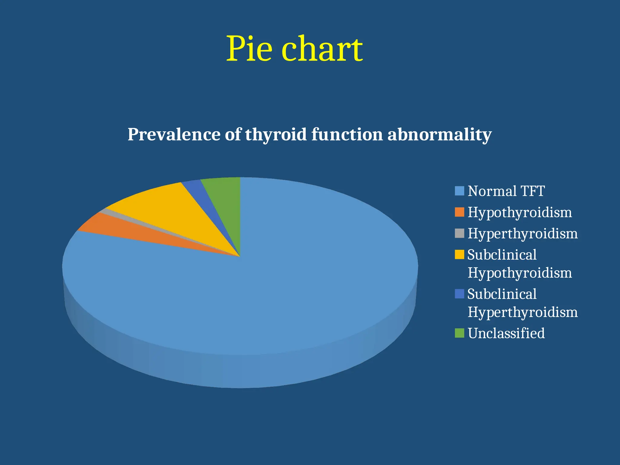
Prevalence of thyroidfunction abnormality
Normal TFT
Hypothyroidism
Hyperthyroidism
Subclinical
Hypothyroidism
Subclinical
Hyperthyroidism
Unclassified
Pie chart
39.
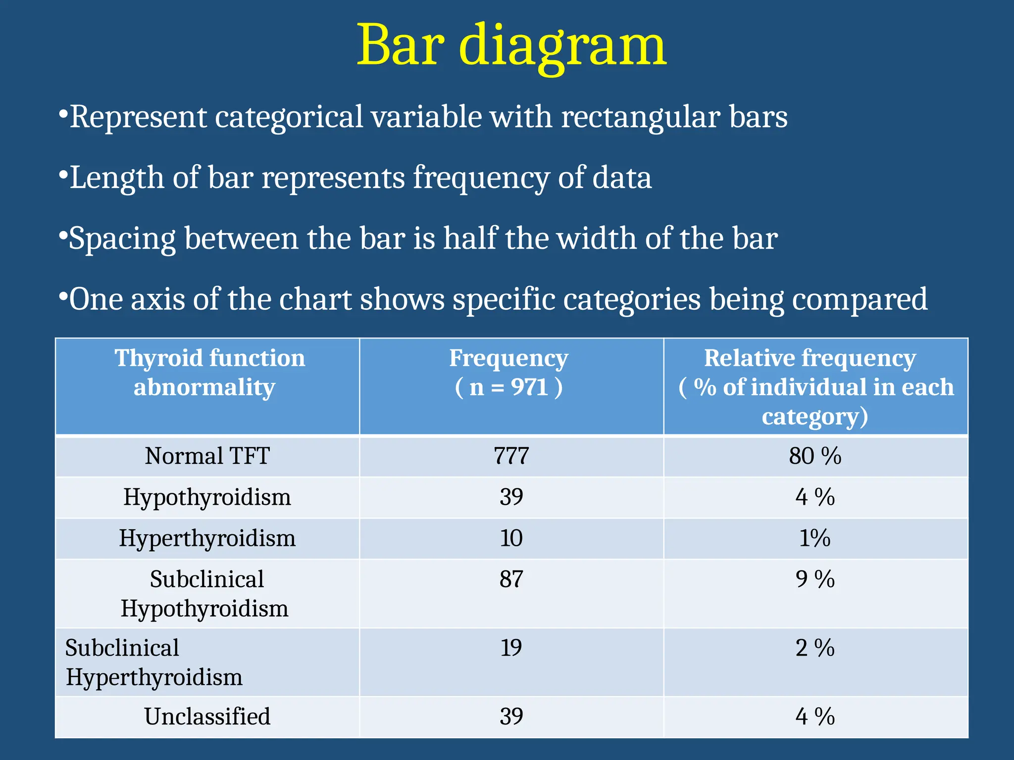
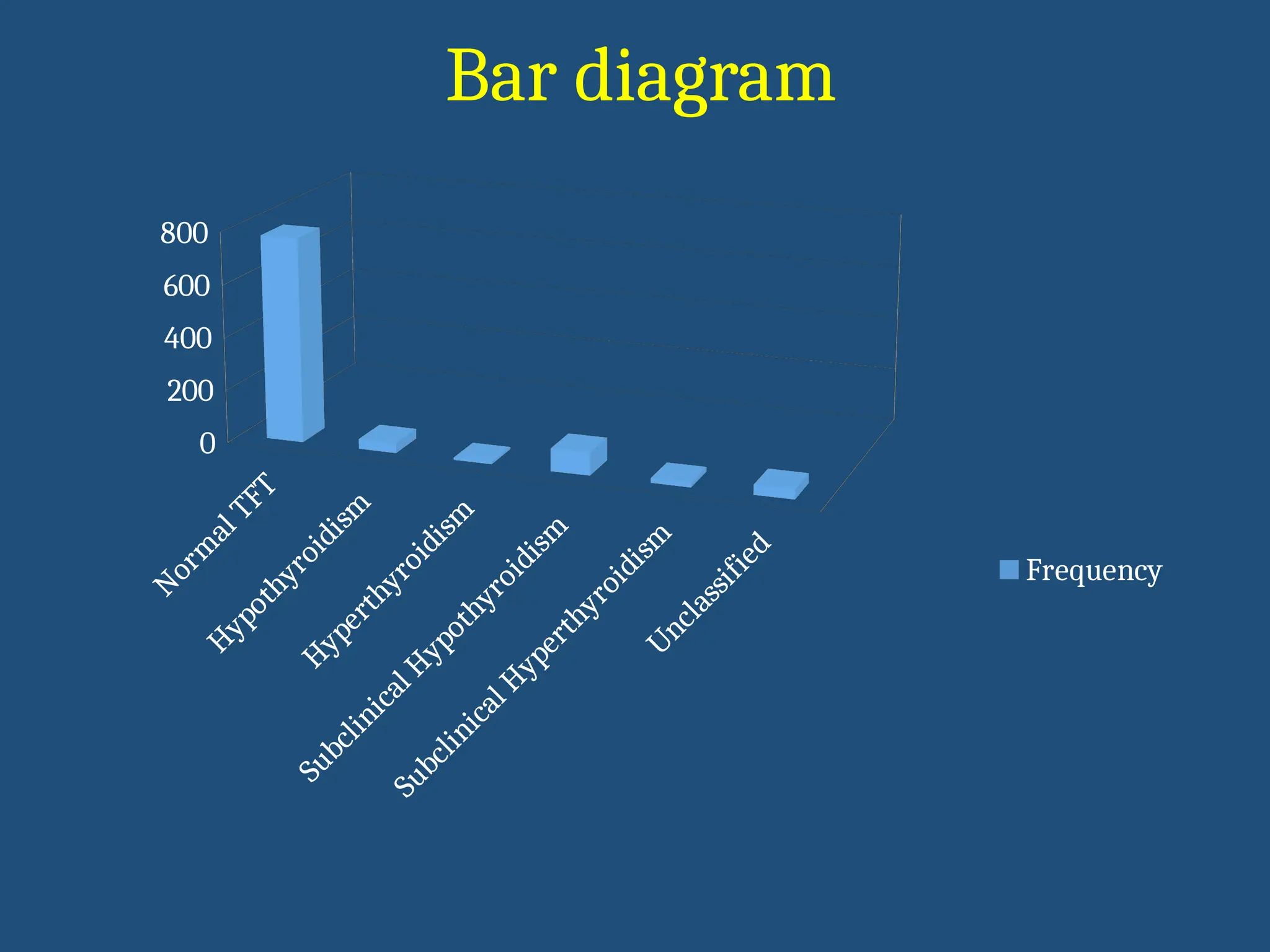
Bar diagram
Thyroid function
abnormality
Frequency
(n = 971 )
Relative frequency
( % of individual in each
category)
Normal TFT 777 80 %
Hypothyroidism 39 4 %
Hyperthyroidism 10 1%
Subclinical
Hypothyroidism
87 9 %
Subclinical
Hyperthyroidism
19 2 %
Unclassified 39 4 %
•Represent categorical variable with rectangular bars
•Length of bar represents frequency of data
•Spacing between the bar is half the width of the bar
•One axis of the chart shows specific categories being compared
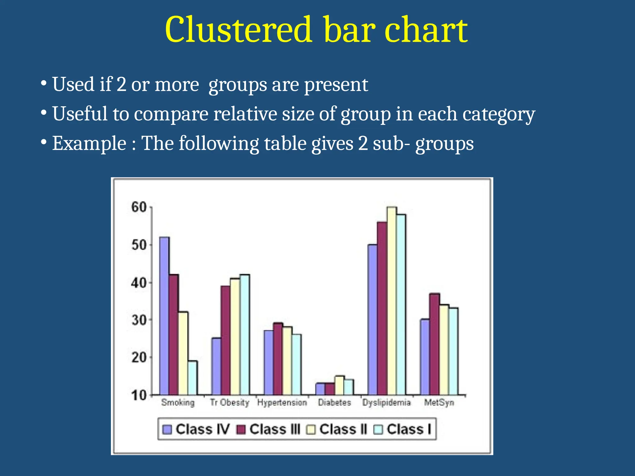
• Used if2 or more groups are present
• Useful to compare relative size of group in each category
• Example : The following table gives 2 sub- groups
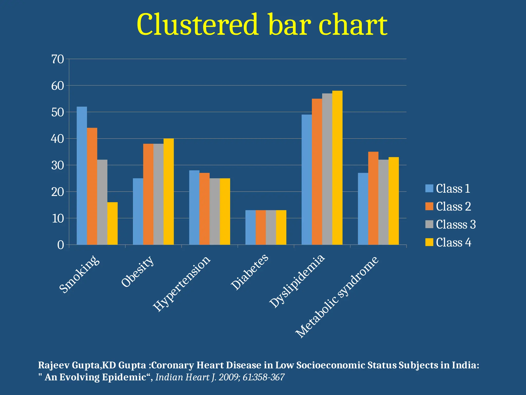
Clustered bar chart
42.
0
10
20
30
40
50
60
70
Class 1
Class 2
Classs3
Class 4
Rajeev Gupta,KD Gupta :Coronary Heart Disease in Low Socioeconomic Status Subjects in India:
" An Evolving Epidemic“, Indian Heart J. 2009; 61:358-367
Clustered bar chart
43.
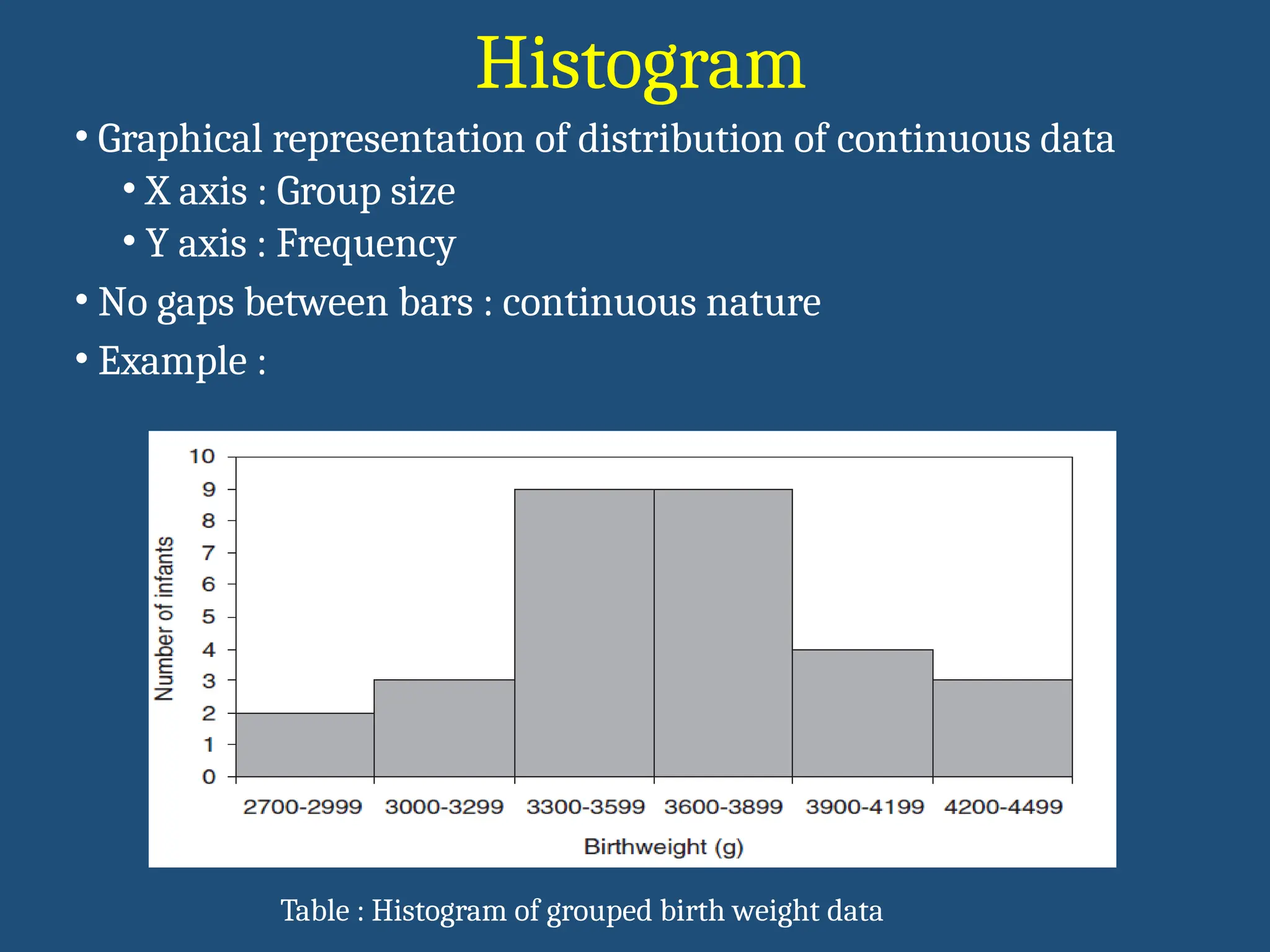
Histogram
• Graphical representationof distribution of continuous data
• X axis : Group size
• Y axis : Frequency
• No gaps between bars : continuous nature
• Example :
Table : Histogram of grouped birth weight data
44.
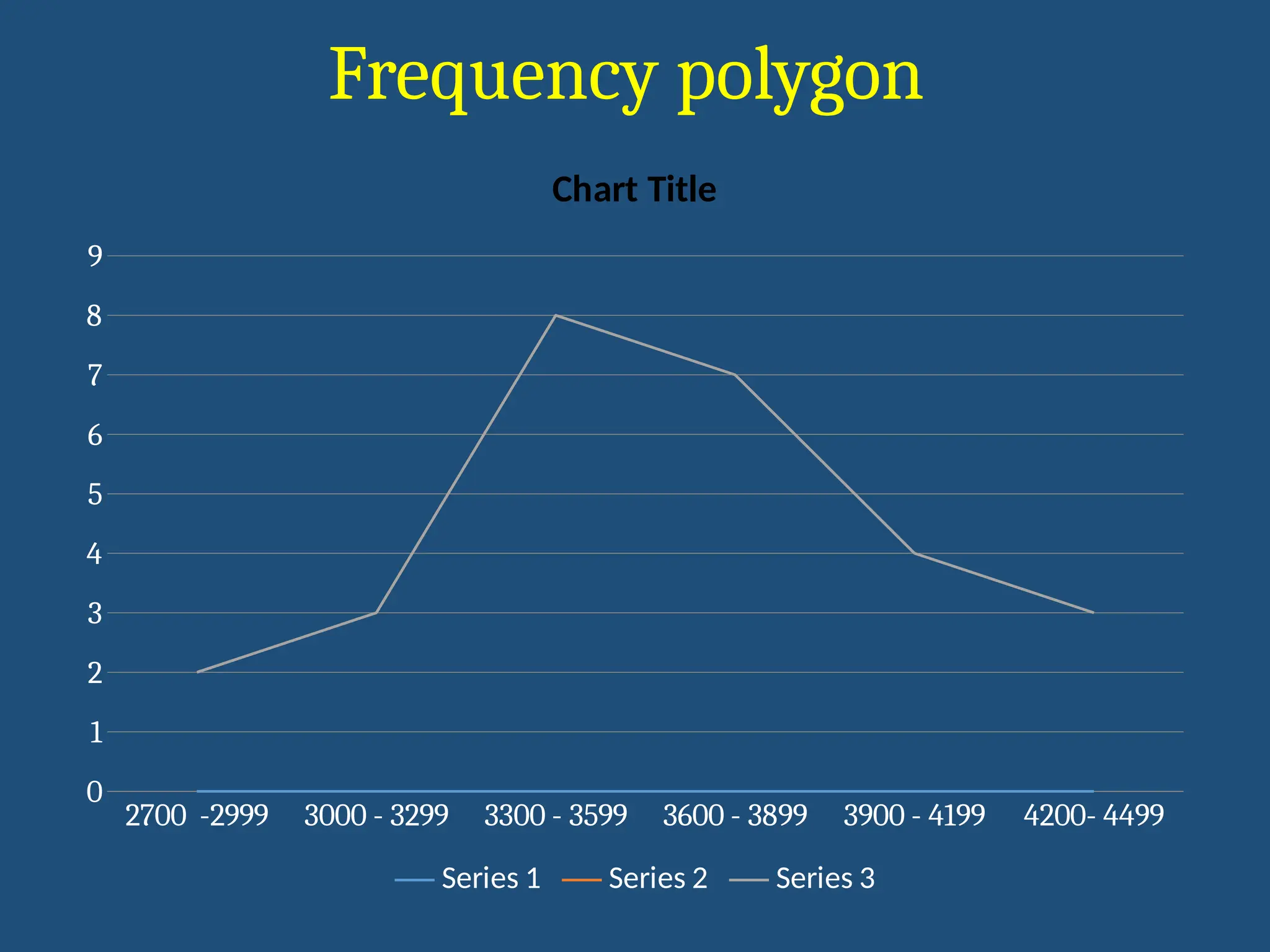
Frequency polygon
• Usefulin comparing 2 frequency distributions
• Developed over histogram
• By joining mid points of class intervals
• At the height of frequency by lines
• When done on
• Large population
- Small intervals
• Smooth curve obtained called frequency curve
45.
Frequency polygon
2700 -29993000 - 3299 3300 - 3599 3600 - 3899 3900 - 4199 4200- 4499
0
1
2
3
4
5
6
7
8
9
Chart Title
Series 1 Series 2 Series 3
46.
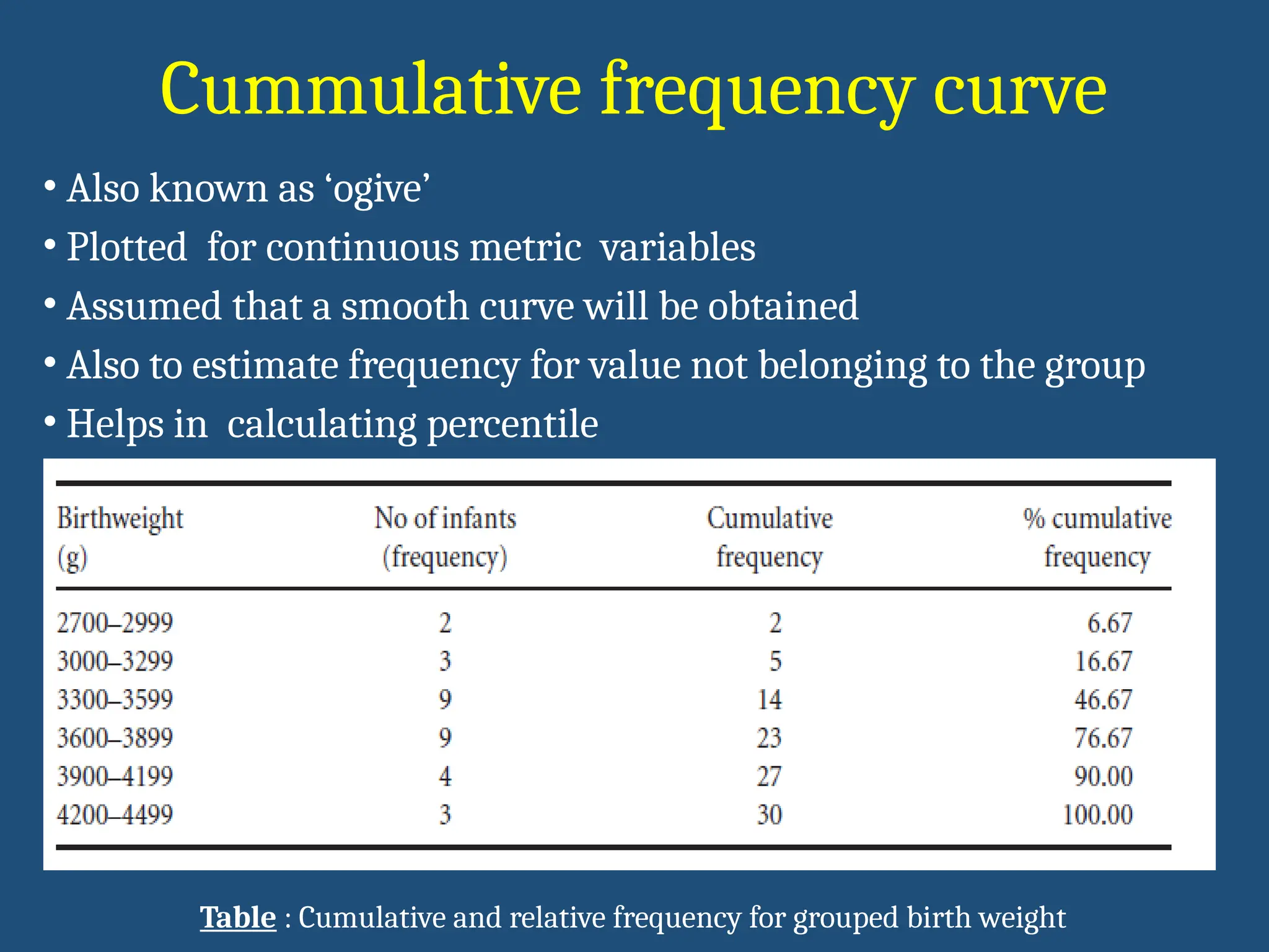
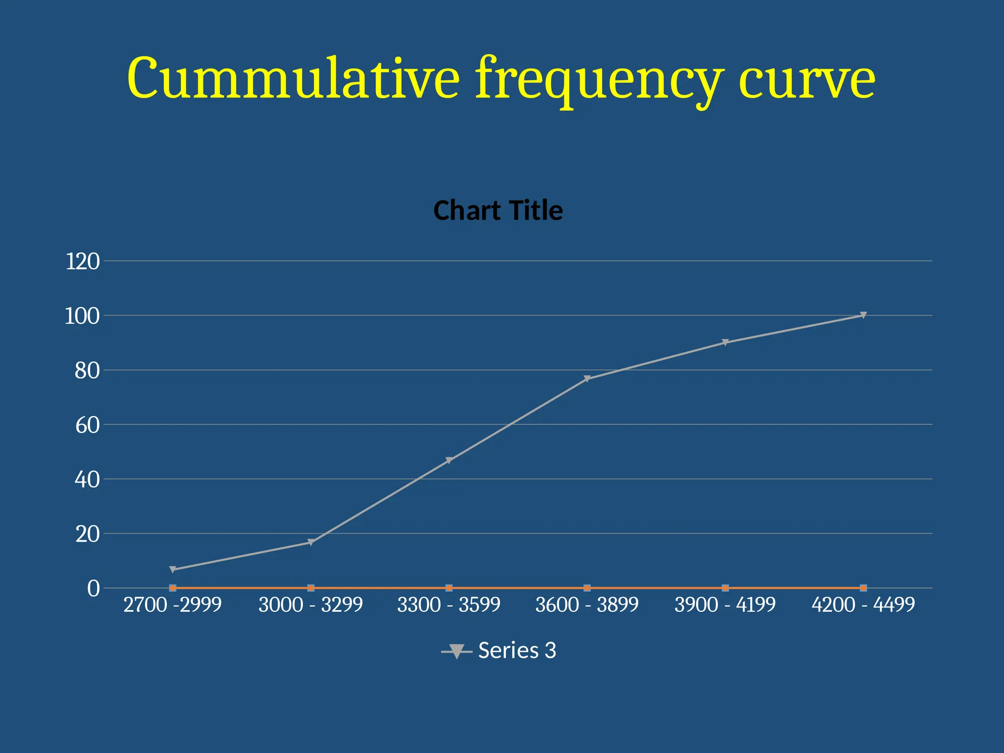
Cummulative frequency curve
•Also known as ‘ogive’
• Plotted for continuous metric variables
• Assumed that a smooth curve will be obtained
• Also to estimate frequency for value not belonging to the group
• Helps in calculating percentile
Table : Cumulative and relative frequency for grouped birth weight
47.
Cummulative frequency curve
2700-2999 3000 - 3299 3300 - 3599 3600 - 3899 3900 - 4199 4200 - 4499
0
20
40
60
80
100
120
Chart Title
Series 3
48.
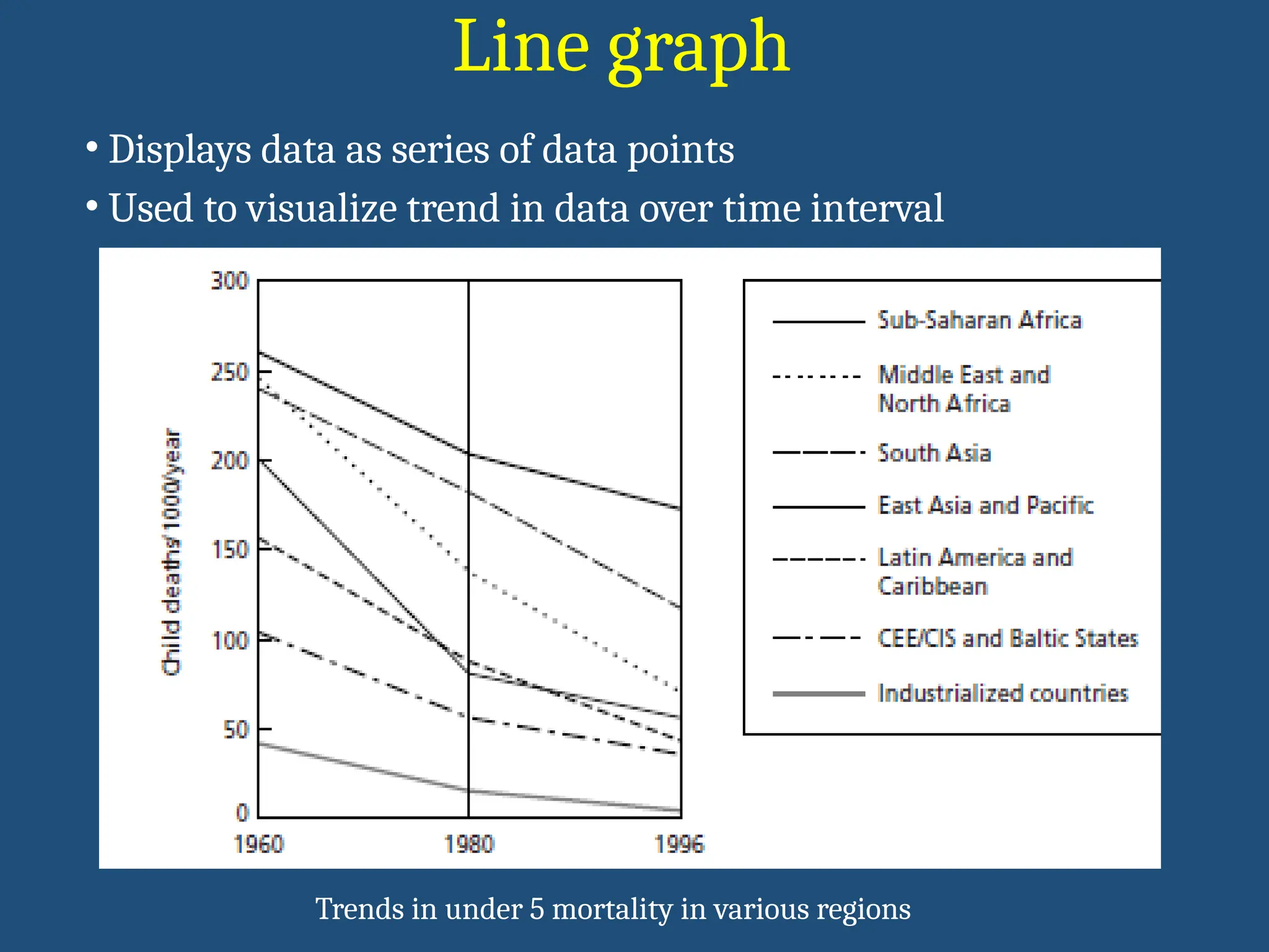
Line graph
• Displaysdata as series of data points
• Used to visualize trend in data over time interval
Trends in under 5 mortality in various regions
49.
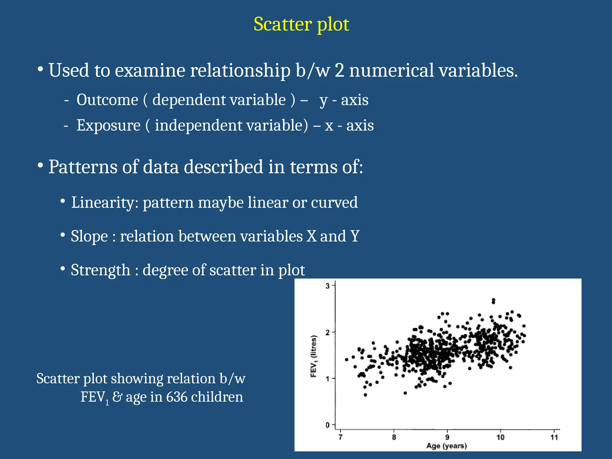
Scatter plot
Scatter plotshowing relation b/w
FEV1 & age in 636 children
• Used to examine relationship b/w 2 numerical variables.
- Outcome ( dependent variable ) – y - axis
- Exposure ( independent variable) – x - axis
• Patterns of data described in terms of:
• Linearity: pattern maybe linear or curved
• Slope : relation between variables X and Y
• Strength : degree of scatter in plot
50.
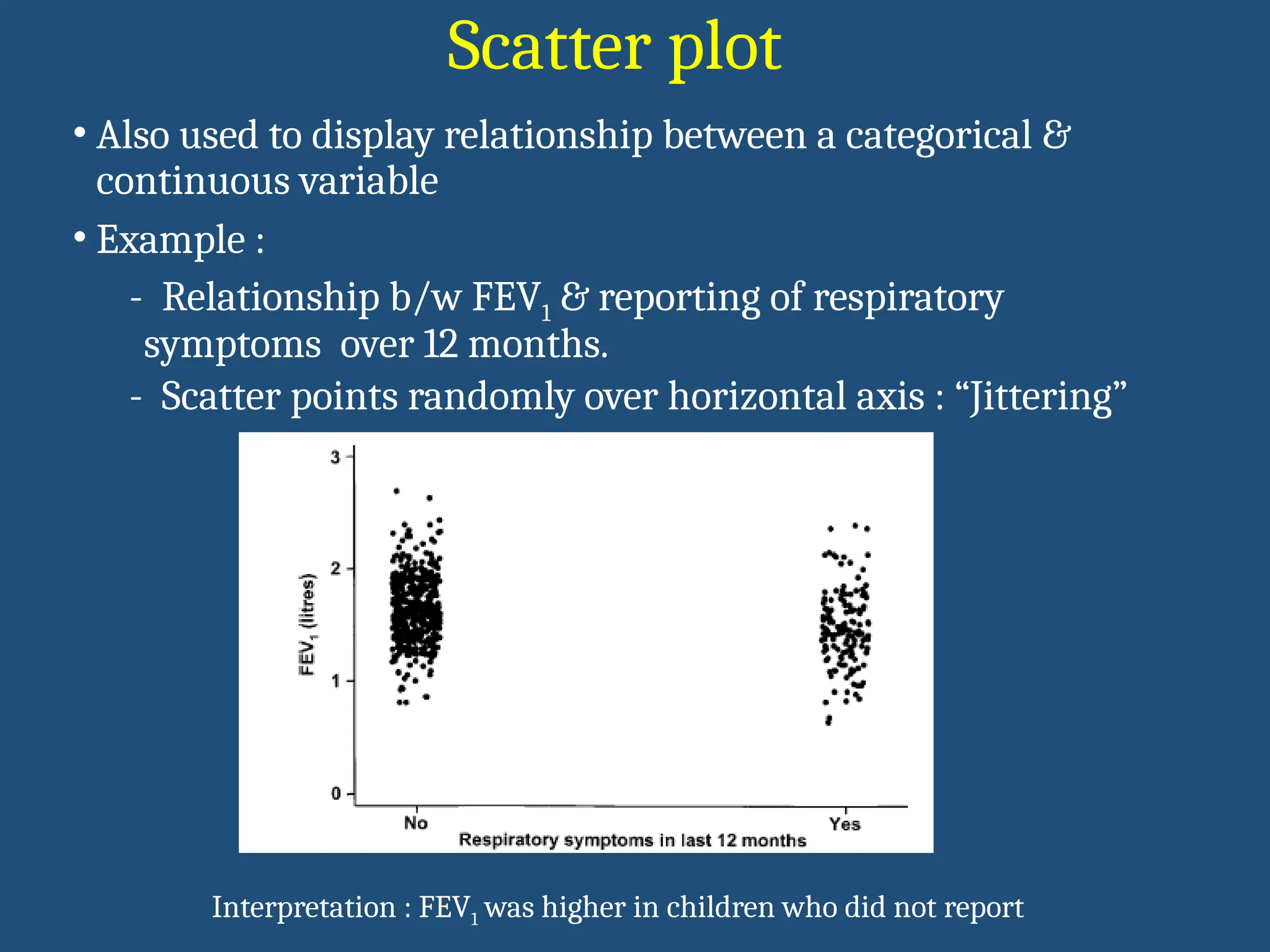
Scatter plot
• Alsoused to display relationship between a categorical &
continuous variable
• Example :
- Relationship b/w FEV1 & reporting of respiratory
symptoms over 12 months.
- Scatter points randomly over horizontal axis : “Jittering”
Interpretation : FEV1 was higher in children who did not report
Data analysis
It involvesthree major steps
•Cleaning and organizing the data for analysis (Data
Preparation)
•Describing the data (Descriptive Statistics)
•Testing Hypotheses and Models (Inferential
Statistics)
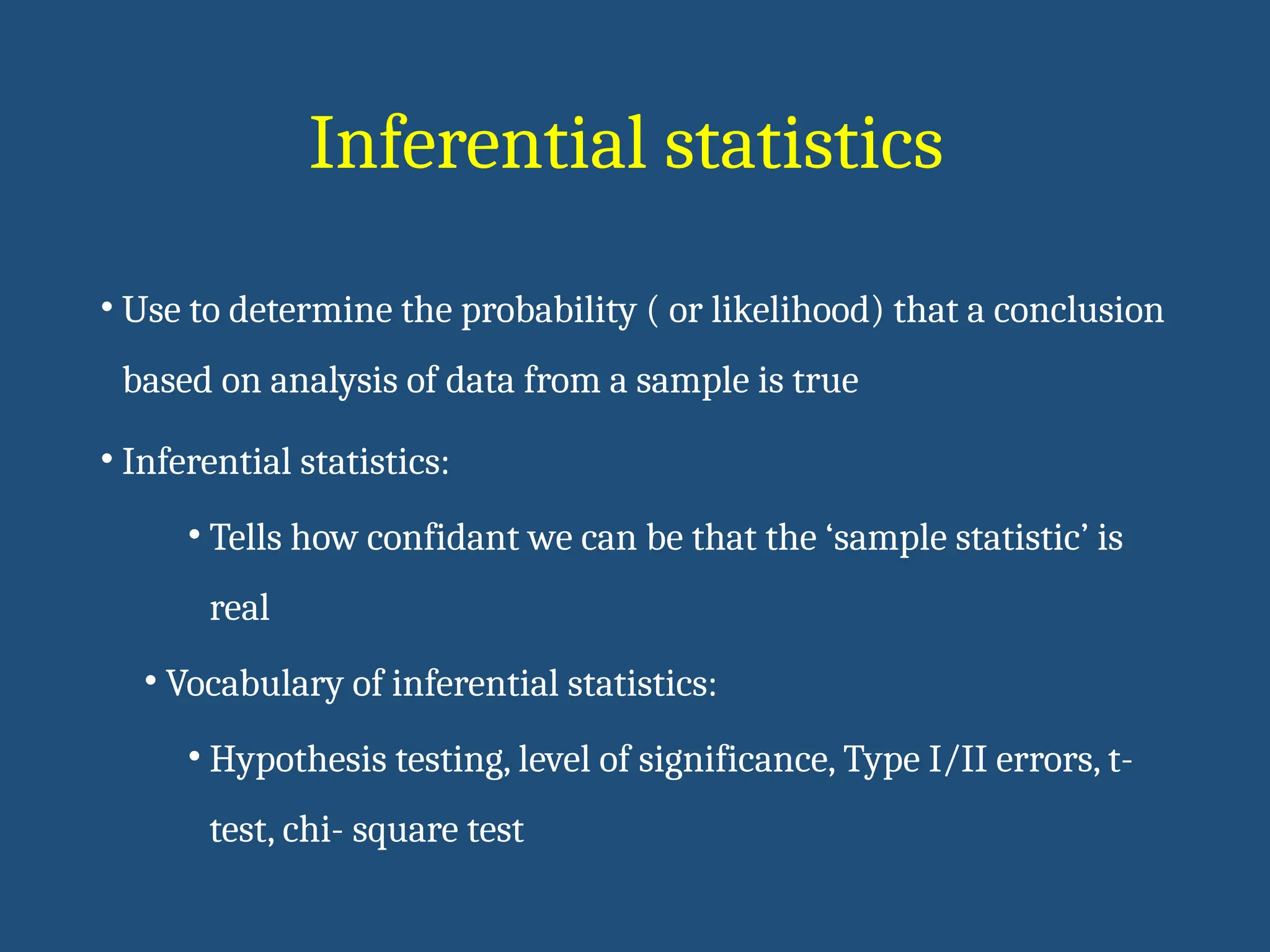
Inferential statistics
• Useto determine the probability ( or likelihood) that a conclusion
based on analysis of data from a sample is true
• Inferential statistics:
• Tells how confidant we can be that the ‘sample statistic’ is
real
• Vocabulary of inferential statistics:
• Hypothesis testing, level of significance, Type I/II errors, t-
test, chi- square test
55.
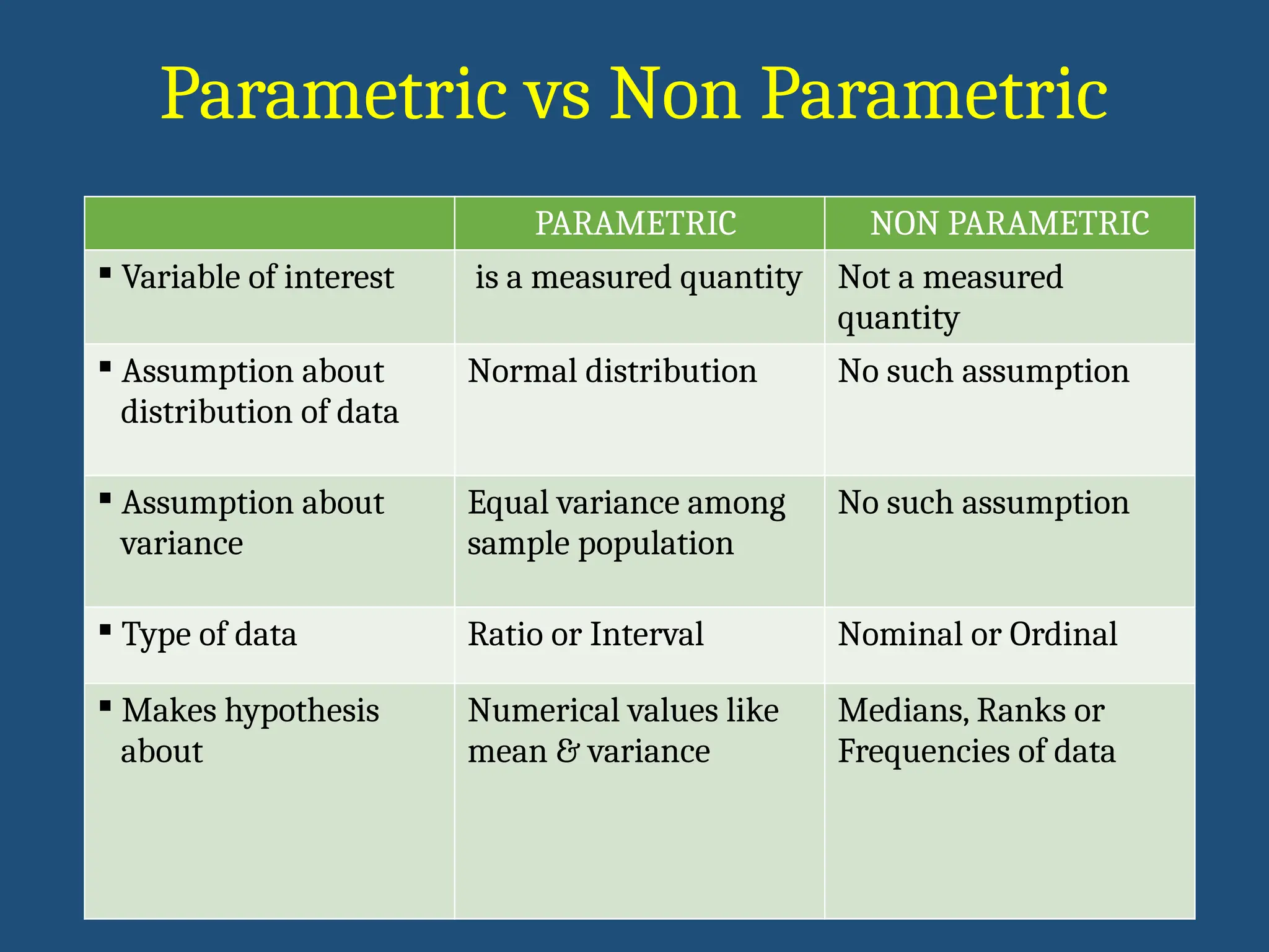
PARAMETRIC NON PARAMETRIC
Variable of interest is a measured quantity Not a measured
quantity
Assumption about
distribution of data
Normal distribution No such assumption
Assumption about
variance
Equal variance among
sample population
No such assumption
Type of data Ratio or Interval Nominal or Ordinal
Makes hypothesis
about
Numerical values like
mean & variance
Medians, Ranks or
Frequencies of data
Parametric vs Non Parametric
56.
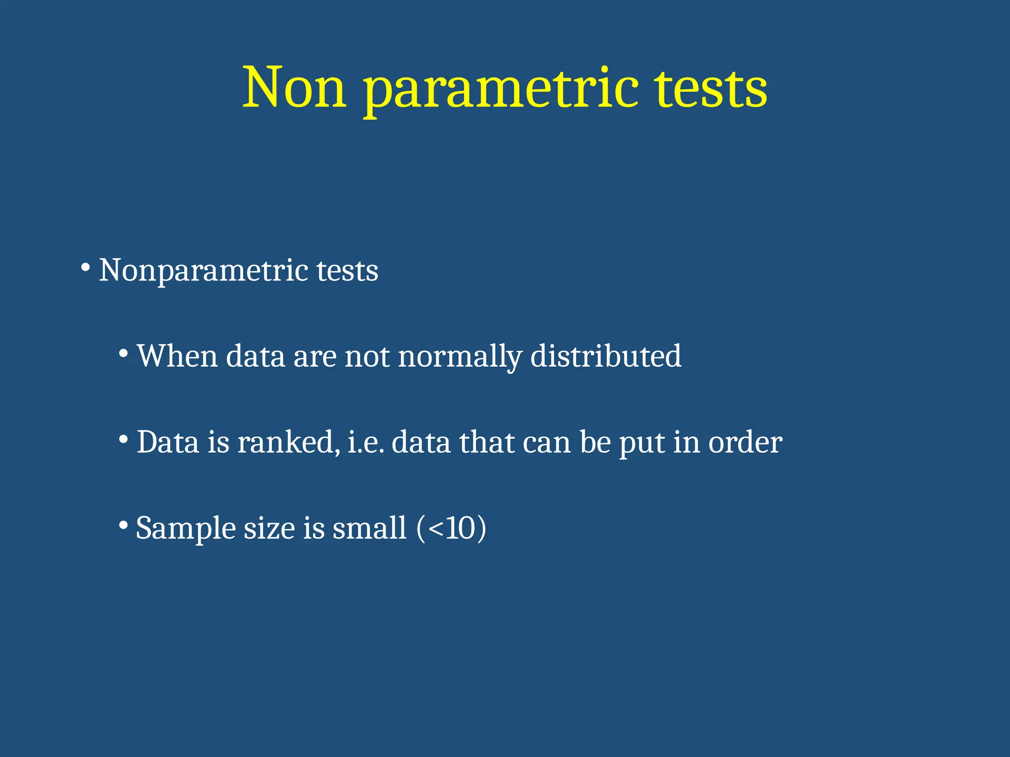
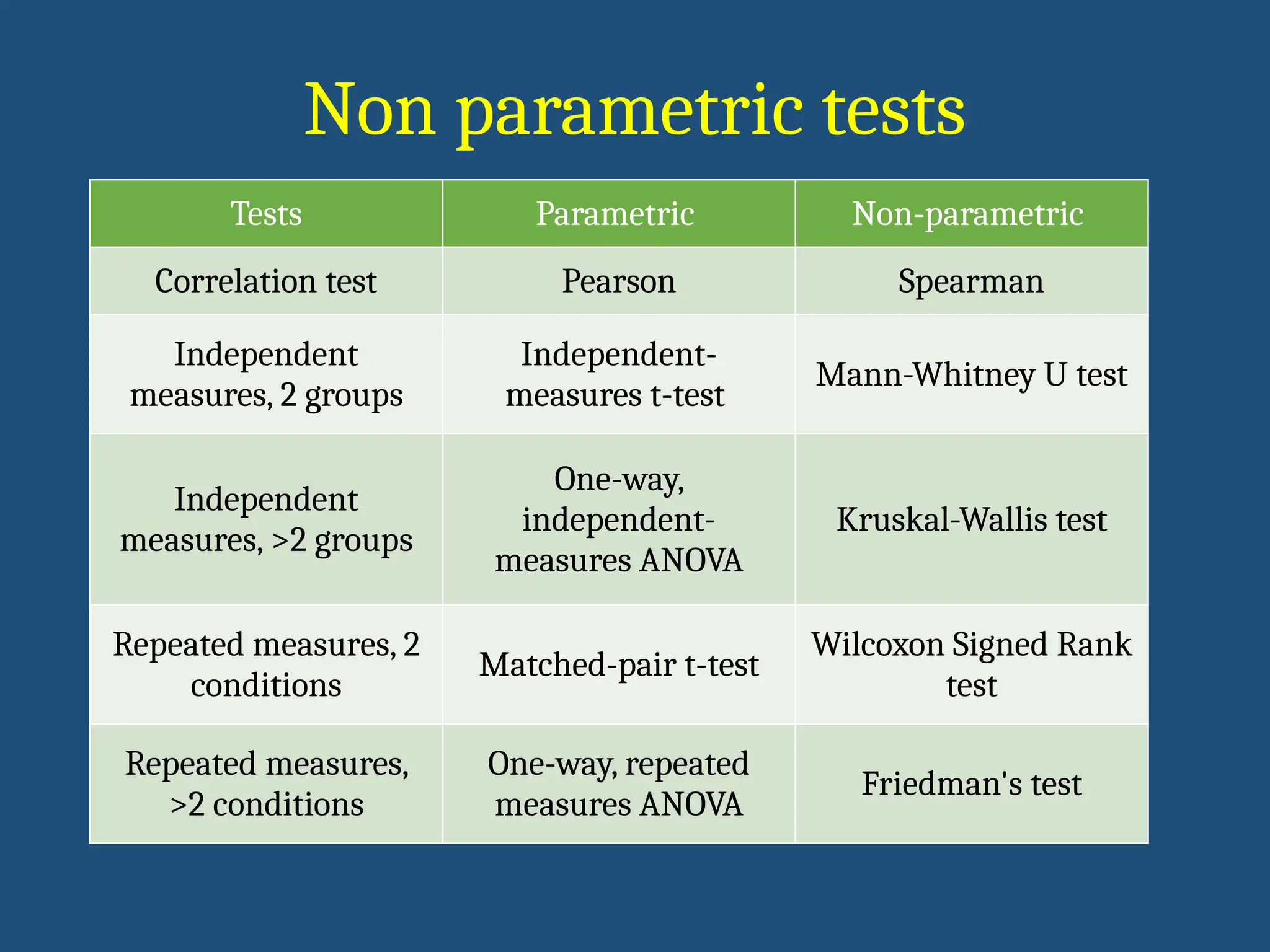
Non parametric tests
•Nonparametric tests
• When data are not normally distributed
• Data is ranked, i.e. data that can be put in order
• Sample size is small (<10)
57.
Tests Parametric Non-parametric
Correlationtest Pearson Spearman
Independent
measures, 2 groups
Independent-
measures t-test
Mann-Whitney U test
Independent
measures, >2 groups
One-way,
independent-
measures ANOVA
Kruskal-Wallis test
Repeated measures, 2
conditions
Matched-pair t-test
Wilcoxon Signed Rank
test
Repeated measures,
>2 conditions
One-way, repeated
measures ANOVA
Friedman's test
Non parametric tests
58.
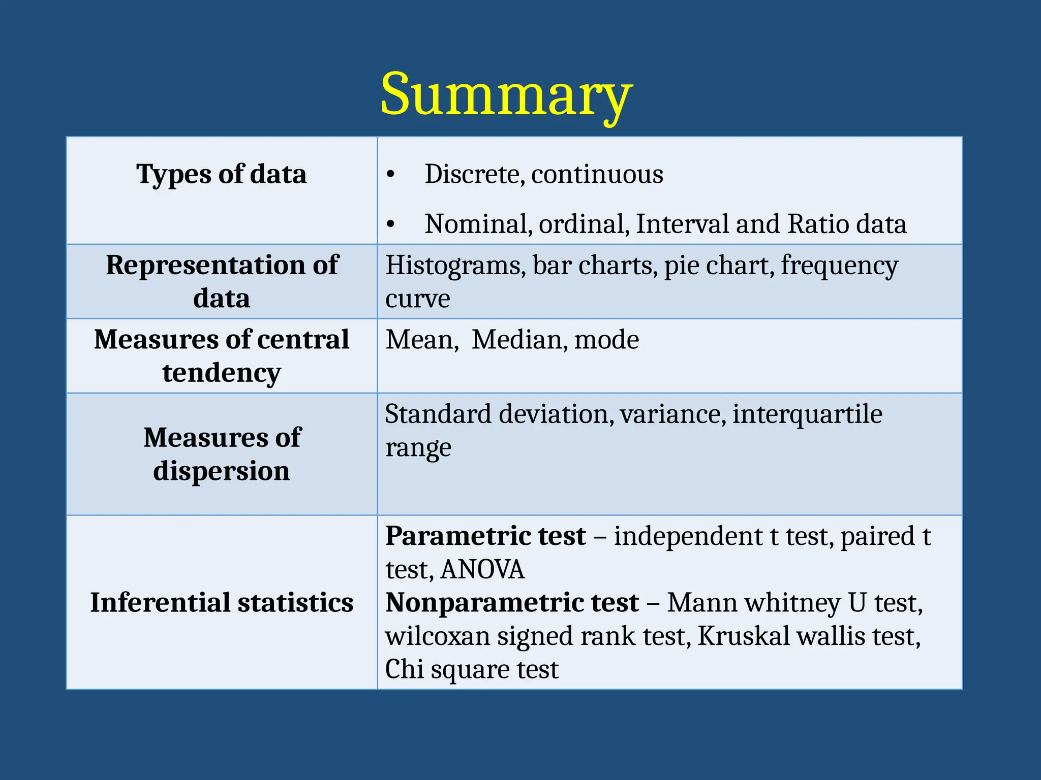
Summary
Types of data• Discrete, continuous
• Nominal, ordinal, Interval and Ratio data
Representation of
data
Histograms, bar charts, pie chart, frequency
curve
Measures of central
tendency
Mean, Median, mode
Measures of
dispersion
Standard deviation, variance, interquartile
range
Inferential statistics
Parametric test – independent t test, paired t
test, ANOVA
Nonparametric test – Mann whitney U test,
wilcoxan signed rank test, Kruskal wallis test,
Chi square test
59.
References
• Norman GR,Streiner D L. Biostatistics: The Bare Essentials. 2nd Edn. B.C. Decker Inc.
2000; p 43-55
• Dawson B, Trapp RG. Basic & Clinical Biostatistics,4th Edn. LANGE basic science. 2004;
p 61-92
• Field A. Discovering statistics using IBM SPSS statistics, 4th
Edn. SAGE. 2014; p 28-34, 54-
8.
• Sedgwick P. Clinical significance Vs statistical significance; BMJ 2014; 348. doi:
http://dx.doi.org/10.1136/bmj.g2130. Accessed on 20-03-2016
• Fethney J. Statistical and clinical significance, and how to use confidence intervals to
help interpret both. Aust Crit Care [Internet]. 2010;23(2):93–7. Available from:
http://dx.doi.org/10.1016/j.aucc.2010.03.001
• LeFebvre R. P Values, Statistical Significance & Clinical Significance. 2011;(Mcid).
Available from:
https://www.uws.edu/wp-content/uploads/2013/10/P_Values_Statistical_Sig_Clinical_
Sig.pdf
• Van Rijn MHC, Bech A, Bouyer J, Van Den Brand JAJG. Statistical significance versus
clinical relevance. Nephrol Dial Transplant. 2017;32:ii6-ii12.
• Baigent C, Landray MJ, Reith C, Emberson J, Wheeler DC, Tomson C, et al. The effects of
lowering LDL cholesterol with simvastatin plus ezetimibe in patients with chronic
kidney disease (Study of Heart and Renal Protection): A randomised placebo-controlled
Editor's Notes
#54 Or determine the likelihood that any conclusion drawn from the data is true
#58 Z score- how far individual value is away from mean by describing its location in SD units


![References
• Norman GR, Streiner D L. Biostatistics: The Bare Essentials. 2nd Edn. B.C. Decker Inc.
2000; p 43-55
• Dawson B, Trapp RG. Basic & Clinical Biostatistics,4th Edn. LANGE basic science. 2004;
p 61-92
• Field A. Discovering statistics using IBM SPSS statistics, 4th
Edn. SAGE. 2014; p 28-34, 54-
8.
• Sedgwick P. Clinical significance Vs statistical significance; BMJ 2014; 348. doi:
http://dx.doi.org/10.1136/bmj.g2130. Accessed on 20-03-2016
• Fethney J. Statistical and clinical significance, and how to use confidence intervals to
help interpret both. Aust Crit Care [Internet]. 2010;23(2):93–7. Available from:
http://dx.doi.org/10.1016/j.aucc.2010.03.001
• LeFebvre R. P Values, Statistical Significance & Clinical Significance. 2011;(Mcid).
Available from:
https://www.uws.edu/wp-content/uploads/2013/10/P_Values_Statistical_Sig_Clinical_
Sig.pdf
• Van Rijn MHC, Bech A, Bouyer J, Van Den Brand JAJG. Statistical significance versus
clinical relevance. Nephrol Dial Transplant. 2017;32:ii6-ii12.
• Baigent C, Landray MJ, Reith C, Emberson J, Wheeler DC, Tomson C, et al. The effects of
lowering LDL cholesterol with simvastatin plus ezetimibe in patients with chronic
kidney disease (Study of Heart and Renal Protection): A randomised placebo-controlled](https://image.slidesharecdn.com/dataanalysisandinterpretation-250703172019-a2ca144b/75/Data-analysis-and-interpretation-ppt-presentation-59-2048.jpg)


![References
• Norman GR, Streiner D L. Biostatistics: The Bare Essentials. 2nd Edn. B.C. Decker Inc.
2000; p 43-55
• Dawson B, Trapp RG. Basic & Clinical Biostatistics,4th Edn. LANGE basic science. 2004;
p 61-92
• Field A. Discovering statistics using IBM SPSS statistics, 4th
Edn. SAGE. 2014; p 28-34, 54-
8.
• Sedgwick P. Clinical significance Vs statistical significance; BMJ 2014; 348. doi:
http://dx.doi.org/10.1136/bmj.g2130. Accessed on 20-03-2016
• Fethney J. Statistical and clinical significance, and how to use confidence intervals to
help interpret both. Aust Crit Care [Internet]. 2010;23(2):93–7. Available from:
http://dx.doi.org/10.1016/j.aucc.2010.03.001
• LeFebvre R. P Values, Statistical Significance & Clinical Significance. 2011;(Mcid).
Available from:
https://www.uws.edu/wp-content/uploads/2013/10/P_Values_Statistical_Sig_Clinical_
Sig.pdf
• Van Rijn MHC, Bech A, Bouyer J, Van Den Brand JAJG. Statistical significance versus
clinical relevance. Nephrol Dial Transplant. 2017;32:ii6-ii12.
• Baigent C, Landray MJ, Reith C, Emberson J, Wheeler DC, Tomson C, et al. The effects of
lowering LDL cholesterol with simvastatin plus ezetimibe in patients with chronic
kidney disease (Study of Heart and Renal Protection): A randomised placebo-controlled](https://crownmelresort.com/image.slidesharecdn.com/dataanalysisandinterpretation-250703172019-a2ca144b/75/Data-analysis-and-interpretation-ppt-presentation-59-2048.jpg)