Download to read offline
![[C II] observations made with the Stratospheric Observatory for
Infrared Astronomy (SOFIA) suggest the N79 South GMC is a
photon-dominated region (PDR) with possible shocks exciting
the CO (16–15) and CO (11–10) emission lines (Nayak et al.
2021). In this work, we are able to resolve the cluster of five
protostars in H72.97-69.39 with Mid-Infrared Instrument
(MIRI)/Medium Resolution Spectroscopy (MRS) observa-
tions. Additionally, we observe two other massive clusters,
one in the South GMC and another in the East GMC. The
source we observe in N79 West is a single protostar. Our
observations reveal how multiple massive YSOs forming
within a cluster affect local gas conditions.
YSOs are enshrouded by dust and gas, which serves as a
reservoir during the main initial accretion phase (McKee &
Ostriker 2007). UV radiation from the central illuminating
source is absorbed and then reradiated at mid- and far-infrared
(IR) wavelengths (Churchwell 2002). The observed IR spectral
emission and absorption lines can reveal the age, mass, and
accretion properties of the central protostar as well as the
temperature and ionized conditions of the surrounding ISM
(Boonman et al. 2003b; Oliveira et al. 2009; Seale et al. 2009;
Rigliaco et al. 2015). Our observations in this work reveal that
objects identified as protostars with previous Spitzer Infrared
Spectrometer (IRS) are actually small clusters, which we can
now resolve with MRS.
We observe a variety of early- and late-stage YSOs in the
South, East, and West GMCs. The spectral features of the six
YSOs we discuss in detail include H2 emission, polyaromatic
hydrocarbon (PAH) emission, silicate absorption, and solid-
and gas-phase ice absorption. Additionally, we observe for the
first time rest-frame mid-IR hydrogen recombination lines
associated with extragalactic star formation with high-resolu-
tion MRS spectra.
The mid-IR H2 originates either from UV radiation from
massive stars or collisional excitation from shocks heating the
molecular gas (Tielens et al. 1993; Hollenbach 1997). The
same UV photons collide with PAH molecules, which in turn
(1) leads to the excitation of various bending and stretching
modes and (2) breaks down large-sized PAH molecules into
smaller ones (Tielens et al. 1993; Peeters et al. 2017). Electrons
ejected from PAH molecules can further heat up the local gas,
(i.e., via the photoelectric effect). Excess H2 emission relative
to PAH emission lines has been observed in active galactic
nuclei (Ogle et al. 2010) and ultraluminous galaxies Higdon
et al. (2006), and it is thought to originate from shocks.
Hydrogen recombination lines are commonly used as a proxy
for accretion rates in YSOs, because of the empirical relation-
ship between H I luminosity and accretion luminosity across a
variety of environments (Calvet et al. 2004; Herczeg &
Hillenbrand 2008). The presence of silicate and ice absorption
lines with little to no H2 and fine-structure emission lines is
indicative of the very young protostars embedded within their
natal gas cloud, where the UV photons from the central star
have yet to ionize the surrounding gas (Oliveira et al. 2013).
The various emission and absorption lines identified in a
spectrum indicate the age of the central protostar as well as
PAH grain size distribution and ionization, plus the origin of
shocks. In this work, we further discuss and interpret the
emission and absorption lines seen in YSOs in N79.
We refer to the four Spitzer-identified sources as W1, E1, S1,
and S2, based on their respective locations in the West, East,
and South GMCs. We call the individual protostars resolved
with MIRI within the Spitzer-identified clusters “YSOs,” with
Y1 located in W1, Y2 and Y3 located in E1, Y4–Y8 in S1, and
Y9–Y11 in S2. In this study, we present MRS observations of
11 YSOs in the N79 region of the LMC, six of which have full
or nearly full mid-IR spectral coverage from 4.9–27.9 μm. The
science goal of this program is to map out the excitation and
physical conditions of the gas in order to better understand
YSO formation at different evolutionary stages. In order to
achieve our science goal, we extract the emission and
absorption lines of the six YSOs with full or nearly full mid-
IR spectral coverage and infer the conditions of the accreting
protostar and the surrounding ISM. Follow-up papers will
model the emission and absorption lines in greater detail.
In Section 2, we describe the source selection strategy and
the observation details. The data processing and resulting
catalog of spectral features are discussed in Section 3. The
Spitzer IRS spectra and photometry of the four MRS
observations are discussed in Section 4, while Section 5 goes
into the details of the YSOs resolved with the JWST MRS
observations. We summarize our results in Section 6.
2. Observation and Source Selection Strategy
We present observations of the N79 region taken with MIRI
(Rieke et al. 2015; Wright et al. 2023) on board JWST as part
of GTO program 1235 (PI: Meixner). The observations were
taken using MRS, an integral field unit (IFU) equipped with
four channels (1, 2, 3, and 4). The channels cover a wavelength
range of 4.90–7.65 μm, 7.51–11.70 μm, 11.55–17.98 μm, and
17.70–27.90 μm, respectively. Channels 1 and 2 have a higher
spectral resolution (R = 2700–3700) in comparison to Chan-
nels 3 and 4 (R = 1600–2800). In contrast, Channels 1 and 2
have a smaller field of view (FOV; 10–20 arcsec2
) in
comparison to Channels 3 and 4 (32–51 arcsec2
; Gardner
et al. 2023). Each Channel is further subdivided into three
subbands (i.e., A, B, and C), which consist of a “SHORT,”
“MEDIUM,” and “LONG” portion of the wavelength range,
respectively. As each MRS Channel possesses the same three
subbands (i.e., 1A, 1B, 1C, 2A, 2B, 2C, etc.), a full spectrum
can therefore be observed with three exposures, typically
accomplished within a single observation setup.
We use the MRS instrument to take observations of SSC
candidate H72.97-69.39, which is a superluminous source with
L = 2.2 × 10⁶
Le, and three other Spitzer-identified massive
YSO candidates in the N79 region (Ochsendorf et al. 2017).
Based on their locations within the N79 South, East, and West
GMCs, we label the Spitzer-identified YSO candidates as S1,
S2, E1, and W1. W1 was observed on 2022 November 14, and
E1 was observed on 2022 November 29. Observations of
H72.97-69.39 (labeled S1) and S2 were taken on 2022
November 30. Figure 1 shows the Spitzer 8 μm observations
of the N79 region and the location of the four MRS
observations.
The SSC candidate H72.97-69.39 was observed with MRS
using the FASTR1 readout mode for a standard four-point
dither pattern, and an assumption that the source is extended.
We use five groups/integration and five integrations/exposure
with a total exposure time for the three subbands SHORT,
MEDIUM, and LONG of 321 s. The three other Spitzer-
identified sources S2, E1, and W1 are observed with the same
readout mode and dither pattern. These YSO candidates are
less luminous than H72.97-69.39, and therefore we use 13
2
The Astrophysical Journal, 963:94 (25pp), 2024 March 10 Nayak et al.](https://image.slidesharecdn.com/nayak2024apj96394-250127005706-08738261/75/JWST-Mid-infrared-Spectroscopy-Resolves-Gas-Dust-and-Ice-in-Young-Stellar-Objects-in-the-Large-Magellanic-Cloud-2-2048.jpg)
![groups/integration and two integrations/exposure for a total
exposure time of 299 s per target.
MRS observations of S1, S2, and E1 show that what was
observed to be a single source with Spitzer is actually a cluster of
two to five less-massive YSOs. Source W1, however, is an
isolated YSO. There are a total of 11 YSOs within the four MRS
observations. We chose a variety of early- and late-stage YSO
candidates based on their spectral features seen with Spitzer IRS
observations.
3. Data Processing
3.1. MIRI MRS Pipeline Processing
The JWST MRS observations were processed using pipeline
version 1.11.0 with jwst_1094.pmap context (Bushouse et al.
2023). This pipeline version uses time-dependent photometric
corrections, has the ability to set the outlier detection kernel
size and threshold, and implements residual fringe correction
during the spectral extraction process. We use the standard
detector corrections calwebb_detector1 and calwebb_spec2
during Stage 1 and Stage 2 of the data reduction process
(Labiano et al. 2016), with the residual_fringe step switched
on. The residual fringe correction step applies additional fringe
correction arising from the difference between fringe pattern on
the detector from an extended source and the standard pipeline
fringe flat. Stage 3 of the pipeline (calwebb_spec3) includes the
outlier_detection and spectrum level residual fringe correction
(ifu_rfcorr) routines. The outlier detection step compares a
median taken from stacked images to the original images, to
determine if there are bad pixels or cosmic rays. We set the size
of the kernel used to normalize the pixel difference in the
outlier detection step to be 11 pixels. Even after the fringe and
residual fringe corrections applied with the standard pipeline
steps, there can still be fringe residuals in extracted spectra; in
particular, there is often high-frequency fringing present in
channels 3 and 4, thought to arise from the dichroics, which are
difficult to remove at the detector level. We used the
(ifu_rfcorr) step on extracted spectra to reduce the contrast of
the fringes that remain.
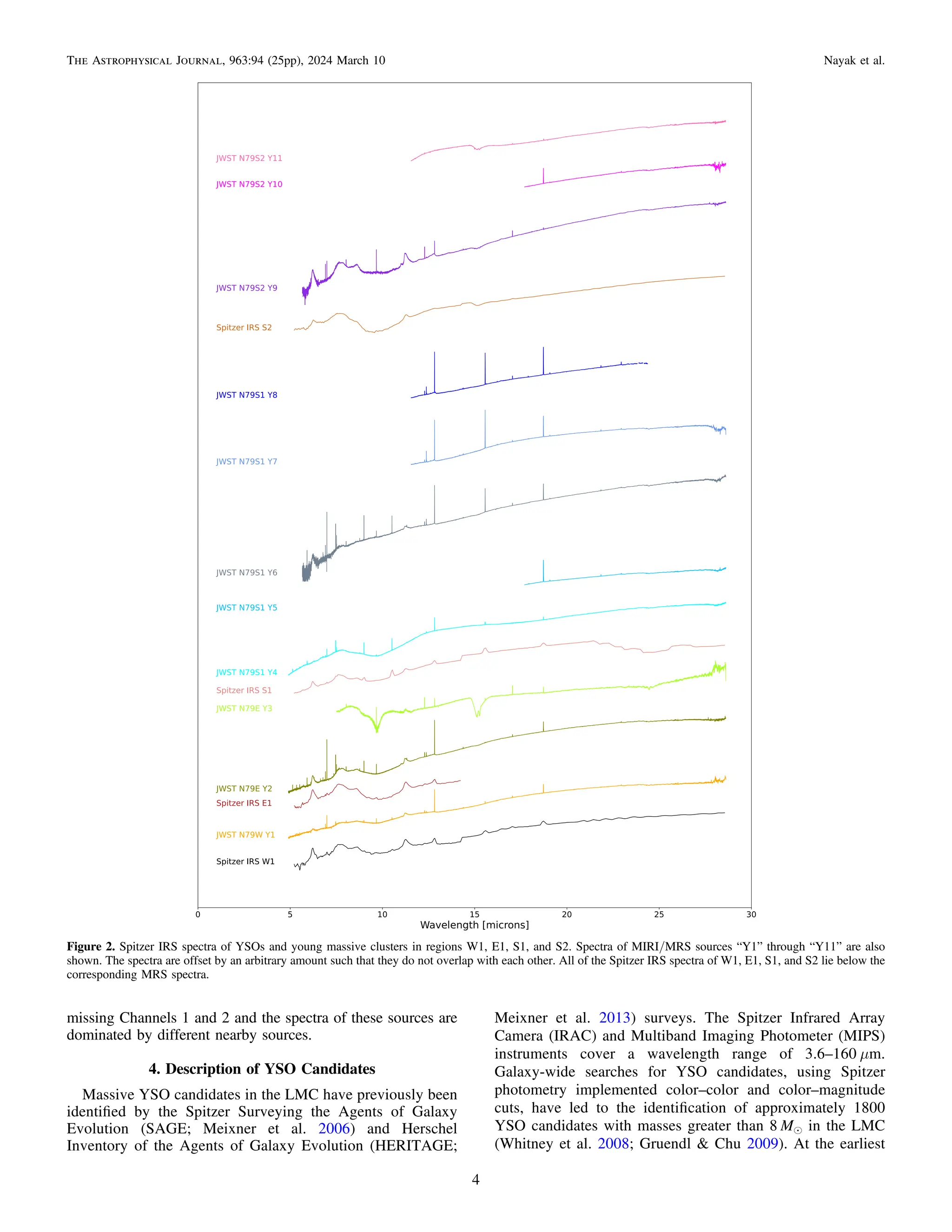
The spectrum of each of the 11 YSOs detected in the four MRS
pointings is extracted with an aperture defined as 1.22 λ/D,
where λ is the wavelength of the IFU cube and D is the beam size.
The background is similarly calculated by extracting a spectrum
within the spectral cube, but away from the bright point sources.
After background subtraction, the 12 spectral cube segments are
scaled in a consecutive manner using a median flux value between
two consecutive subbands such that channel 1B is scaled to 1A,
and then channel 1C is scaled to 1B, and so forth. The resulting
spectral segments are stitched together using the combine_1d step
of the JWST pipeline. Figure 2 shows the MRS spectra of the 11
sources in this work as well as Spitzer IRS spectra of S1, S2, E1,
and W1.
We fit a continuum to the spectra extracted in each subband
using the spline function in the astropy package. After subtracting
the continuum, the emission and absorption lines are detected with
find_lines_threshold function from specutils. The lines are fit with
a Gaussian profile, and their parameters (measured wavelength,
uncertainty in wavelength, FWHM, flux, and uncertainty in flux)
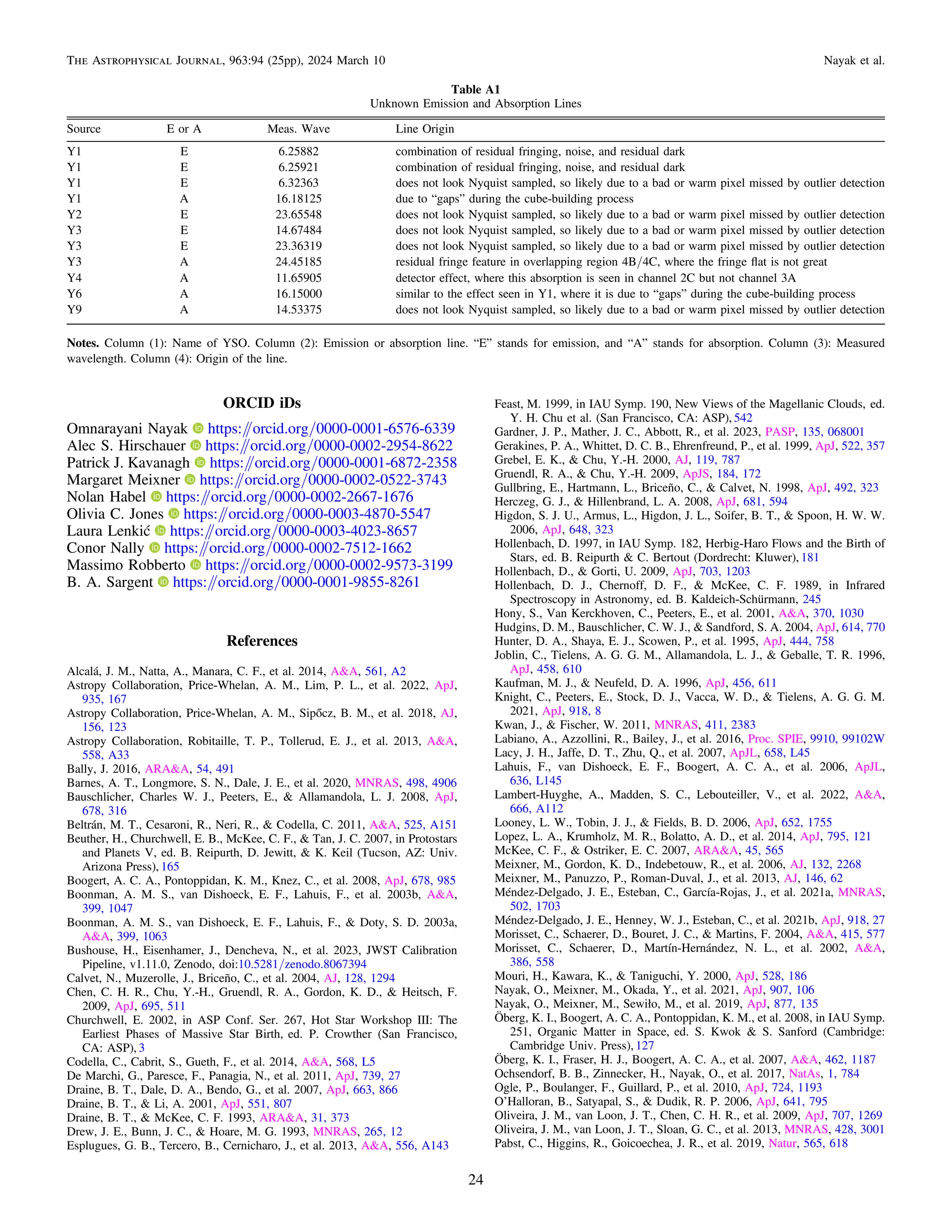
are listed in Tables 1–6. Table 7 summarizes the emission and
absorption lines seen in the spectra of Y1, Y2, Y3, Y4, Y6,
and Y9. Taking into account the radial velocity of N79
(235 km s−1
; Nayak et al. 2019), the narrow emission and
absorption features are matched to the closest known H2, HI, fine-
structure, or ice lines within 0.01 μm. If there are multiple
matches, then the closest laboratory emission or absorption line is
selected to be the observed line. The broad PAH emission line and
ice absorption lines are determined by matching the observed
features to the known laboratory lines, with the requirement that
λobserved − λlaboratory < 0.05. We list the emission and absorption
lines we are unable to identify in Appendix Table A1; these are
due to warm pixels, fringe flat correction issues, undersampling,
and stitching effects in overlap channels.
3.2. Catalog of Spectral Features
Figures 3–6 show cube slices at 5.51, 6.20, 11.20, 12.81,
17.04, and 18.71 μm, which trace H2 5.51 μm, PAH features,
[Ne II], H2 17.04 μm, and [S III] emission lines, respectively.
The YSOs in each region are labeled Y1 through Y11. The
spectra for YSOs Y1 located in the N79 West GMC, Y2 in the
East GMC, and Y4 in the South GMC observation cover the
full MRS wavelength range from 4.9–27.9 μm. Y3 located in
N79 East is very faint in Channel 1. The extracted spectrum for
this source is noisy, with little to no signal in wavelengths
shorter than 7.5 μm. Sources Y6 in S1 and Y9 in S2 are noisy
in Channel 1A, and therefore the spectra shown for these two
sources in Figure 2 are for 1B and longer wavelengths. YSOs
Y5, Y7, and Y8 are on the edge of the MRS FOV in Channels
1 and 2 (Figure 5); therefore, they do not have the full spectral
coverage. Additionally, the emission lines seen in YSOs Y5,
Y7, and Y8 are the same as the emission lines seen in Y6,
which can be seen in Figure 2. The similarity in emission line
species and line strength between the three YSOs in region S1
to Y6 implies the three protostars are not the dominating source
in the MRS FOV. Y10 and Y11 are also on the edge of
Channel 1, which is shown in Figure 6, and therefore they do
not have full spectral coverage of MRS.
In this work, we discuss sources Y1, Y2, Y3, Y4, Y6, and
Y9 in further detail. Sources Y5, Y7, Y8, Y10, and Y11 are
Figure 1. Spitzer IRAC 8.0 μm image of the N79 region. We highlight the
location of the MRS footprint with the four red circles. The red circles have a
diameter of 70″, much larger than the MRS footprint. We selected these four
sources because previous Spitzer IRS spectral observations indicated these are
indeed YSOs, in addition to SED models indicating that these YSOs are very
massive (over 8 Me).
3
The Astrophysical Journal, 963:94 (25pp), 2024 March 10 Nayak et al.](https://image.slidesharecdn.com/nayak2024apj96394-250127005706-08738261/75/JWST-Mid-infrared-Spectroscopy-Resolves-Gas-Dust-and-Ice-in-Young-Stellar-Objects-in-the-Large-Magellanic-Cloud-3-2048.jpg)
![stages of formation, YSOs are enshrouded by dust and gas.
Their radiation is absorbed by the dust and gas, and
subsequently reprocessed to output emission at far-IR
wavelengths. Herschel Photoconductor Array Camera and
Spectrometer (PACS) and Spectral and Photometric Imaging
Receiver (SPIRE) data cover the far-IR wavelength range of
70–500 μm, allowing for the identification of the youngest
and most-embedded YSO candidates. Seale et al. (2014)
found 2493 YSO candidates using Spitzer and Herschel
photometry, 73% of which were not identified with previous
studies that only used Spitzer.
The angular resolution of Spitzer and Herschel ranges from
1 7 in the IRAC 3.6 μm band to 40 5 in the SPIRE 500 μm
band. Channel 1 MIRI/MRS observations have an FOV that is
3 2 × 3 7. Our MRS observations reveal that what appeared
to be a single YSO in Spitzer and Herschel observations is
actually a small cluster of YSOs in S1, S2, and E1. MRS
observations of W1 reveal a single YSO.
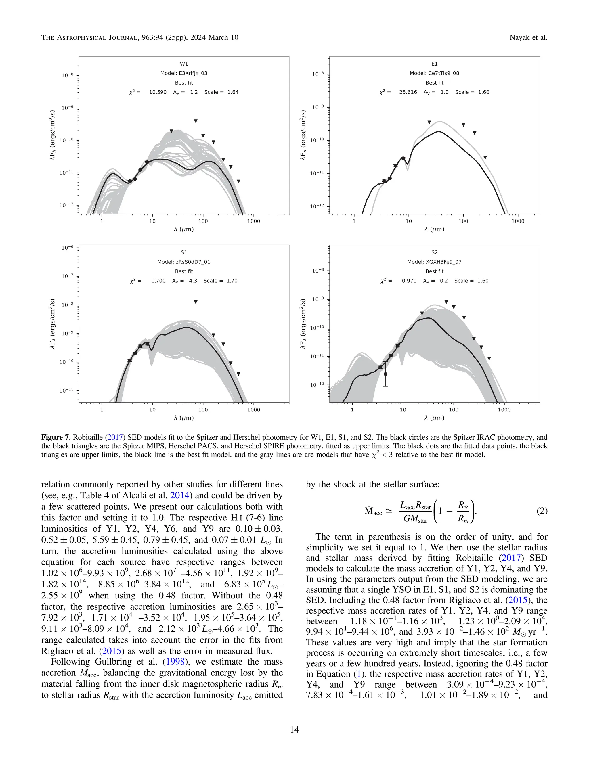
We use the Spitzer and Herschel photometry from Gruendl
& Chu (2009) and Seale et al. (2014) to fit spectral energy
distribution (SED) models to get estimates of the total masses
and luminosities of the clusters in E1, S1, and S2, and of the
isolated YSO in W1. The “spbhmi” Robitaille (2017) SED
model grid used in this work includes 10,000 model YSOs with
a wide range of parameters: stellar radius (0.1–100 Re), stellar
temperature (2000–30,000 K), disk mask (10−8
–10−1
Me),
outer disk radius (50–5000 au), envelope density
(10−24
–10−16
g cm−3
), envelope power law (−2 to −1), cavity
density (10−23
–10−20
g cm−3
), and cavity opening angle (0°–
60°). Figure 7 shows the Robitaille (2017) best-fit SED models
Table 1
Source Y1 Emission and Absorption Lines
Name Absorption or Lab Wave Meas Wave Meas Wave Err FWHM Flux Flux Err
Emission (μm) (μm) (μm) (μm) (erg s−1
cm−2
) (erg s−1
cm−2
)
H2 10-9 Q(2) E 4.987 4.99115 0.00125 0.00093 8.815E-17 1.122E-16
H I (10-6) E 5.129 5.13902 0.00138 0.00138 5.369E-17 1.070E-16
H2 5-5 S(13) E 5.291 5.29989 0.00109 0.00129 1.005E-16 1.079E-16
[Fe II] a4F9/2-a6D9/2 E 5.340 5.34462 0.00013 0.00136 3.631E-16 1.145E-16
H2 7-6 O(6) E 5.415 5.42082 0.00012 0.00657 3.573E-16 1.121E-16
H2 0-0 S(7) E 5.511 5.51660 0.00100 0.00176 2.348E-16 1.030E-16
H2 9-8 Q(13) E 5.909 5.91066 0.00174 0.00167 1.135E-16 1.231E-16
NH3 A 6.150 6.12035 0.00033 0.00437 4.060E-16 1.043E-16
PAH E 6.200 6.22776 0.00077 0.10208 2.972E-14 7.087E-16
[Ni II] 2D3/2-2D5/2 E 6.636 6.64202 0.00122 0.00232 1.319E-16 1.029E-16
H2 0-0 S(5) E 6.910 6.91495 0.00025 0.00208 7.061E-16 1.035E-16
[Ar II] 2P1/2-2P3/2 E 6.985 6.99076 0.00044 0.00199 3.713E-15 1.367E-16
C2H5OH A 7.240 7.22451 0.00035 0.00661 4.094E-16 8.805E-17
H2 8-8 S(12) E 7.323 7.33174 0.00346 0.00124 9.381E-17 9.875E-17
H2 10-9 Q(13) E 7.452 7.46514 0.00046 0.00230 7.573E-16 1.078E-16
H2 11-9 O(14) E 7.507 7.50931 0.00131 0.00197 1.026E-16 1.039E-16
PAH E 7.700 7.64696 0.00649 0.12591 5.838E-14 9.781E-16
PAH E 7.700 7.84175 0.00857 0.11913 5.252E-14 8.866E-16
H2 0-0 S(4) E 8.025 8.03197 0.00002 0.00208 4.252E-16 2.013E-16
PAH E 8.600 8.64508 0.00313 0.60429 1.569E-13 2.585E-15
[Ar III] 3P1-3P2 E 8.991 8.99895 0.00070 0.00294 4.512E-16 1.470E-16
H2 3-3 S(4) E 9.431 9.43722 0.00087 0.00161 7.016E-17 1.111E-16
H2 0-0 S(3) E 9.665 9.67298 0.00003 0.00257 9.457E-16 1.093E-16
[S IV] 2P3/2-2P1/2 E 10.511 10.51908 0.00013 0.00331 3.934E-16 1.959E-16
PAH E 11.000 11.00937 0.01351 0.04045 2.485E-15 2.633E-15
PAH E 11.200 11.25099 0.00086 0.12722 5.593E-14 1.194E-15
(9-7) E 11.310 11.31906 0.00191 0.00306 3.124E-16 8.245E-17
H2 0-0 S(2) E 12.279 12.28917 0.00042 0.00358 6.591E-16 2.709E-16
H I (7-6) E 12.370 12.38198 0.00073 0.00458 1.289E-15 3.953E-16
PAH E 12.700 12.759794 0.00363 0.24805 3.061E-14 1.423E-15
[Ne II] 2P1/2-2P3/2 E 12.814 12.82427 0.00052 0.00430 3.216E-14 6.875E-16
H2 5-4 O(15) E 13.828 13.84260 0.00115 0.00306 7.150E-17 2.483E-16
[Cl II] 3P1-3P2 E 14.368 14.37880 0.00005 0.00424 3.582E-16 2.608E-16
[Ne III] 3P1-3P2 E 15.555 15.56790 0.00085 0.00640 1.750E-15 2.698E-16
PAH E 16.400 16.43141 0.00355 0.08704 6.57E-15 8.51E-16
H2 0-0 S(1) E 17.035 17.04974 0.00099 0.00576 2.091E-15 3.982E-16
[P III] 2P3/2-2P1/2 E 17.885 17.89816 0.00058 0.00641 3.619E-16 4.472E-16
[Fe II] a4F7/2-a4F9/2 E 17.936 17.94813 0.00201 0.00667 6.665E-16 3.848E-16
[S III] 3P2-3P1 E 18.713 18.72723 0.00178 0.00938 3.702E-14 2.742E-15
[Fe III] 5D3-5D4 E 22.925 22.94277 0.00023 0.00936 2.592E-15 2.031E-15
[Fe II] a6D7/2-a6D9/2 E 25.998 26.01579 0.00101 0.01069 8.920E-15 2.534E-15
Notes. Column (1): Name of line. Column (2): Emission or absorption line. “E” stands for emission, and “A” stands for absorption. Column (3): Laboratory
wavelength. Column (4): Measured wavelength. Column (5): Error in measured wavelength. Column (6): FWHM of line. Column (7): Measured flux. Column (8):
Error in flux.
5
The Astrophysical Journal, 963:94 (25pp), 2024 March 10 Nayak et al.](https://image.slidesharecdn.com/nayak2024apj96394-250127005706-08738261/75/JWST-Mid-infrared-Spectroscopy-Resolves-Gas-Dust-and-Ice-in-Young-Stellar-Objects-in-the-Large-Magellanic-Cloud-5-2048.jpg)
![fit to the observed mid-IR and far-IR data. The Spitzer IRAC
observations are in black circles, and the Spitzer MIPS and
Herschel observations are in black triangles, fitted as upper
limits. The beam sizees of the Spitzer MIPS, Herschel PACS,
and Herschel SPIRE observations range from 6″–35″ (Meixner
et al. 2006, 2013). Mid- and far-IR emission from the central
protostar and the surrounding dust will be unresolved by the
MIPS, PACS, and SPIRE, due to the beam size being much
larger than the 1″–2″ beam size of IRAC (Meixner et al. 2006).
Therefore, the mid- and far-IR photometry are fit as upper
limits when we use the SED models. The best-fit models for
sources E1, S1, and S2 show a rise in flux toward mid-IR
wavelengths, which is typical for YSOs. The best-fit model for
source W1 is a more evolved YSO, as inferred from the SED:
There is some IR emission seen with the bump around 100 μm;
however, the optical light from the star is also seen in the SED
with the bump around 10 μm.
The masses of clusters E1, S1, S2, and the isolated YSO Y1
in W1 determined by fitting the SEDs with Robitaille (2017)
models are 18.3 ± 2.7, 25.4 ± 3.2, 15.7 ± 4.5, and 13.6 ±
1.6 Me, respectively. The luminosities of E1, S1, S2, and
W1 are 4.1 ± 1.9 × 10⁴
, 1.2 ± 0.5 × 10⁵
, 3.1 ± 1.2 × 10⁴
, and
Table 2
Source Y2 Emission and Absorption Lines
Name Absorption or Lab Wave Meas Wave Meas Wave Err FWHM Flux Flux Err
Emission (μm) (μm) (μm) (μm) (erg s−1
cm−2
) (erg s−1
cm−2
)
H I (10-6) E 5.129 5.13263 0.00057 0.00182 4.748E-16 6.219E-17
[Fe II] a4F9/2-a6D9/2 E 5.340 5.34461 0.00006 0.00137 5.551E-16 8.300E-17
H2 9-8 Q(11) E 5.373 5.38499 0.00059 0.00167 9.680E-17 4.856E-17
H2 0-0 S(7) E 5.511 5.51671 0.00111 0.00173 2.866E-16 4.758E-17
H2 8-7 Q(15) E 5.540 5.53164 0.00244 0.00185 1.542E-16 4.724E-17
H I (15-7) E 5.711 5.71989 5.71989 0.00151 1.464E-16 4.922E-17
H2 9-8 Q(13) E 5.909 5.91320 0.00000 0.00210 8.560E-16 7.946E-17
H2 7-6 O(7) E 5.956 5.96141 0.00021 0.00198 1.063E-16 5.994E-17
H2 0-0 S(6) E 6.109 6.11391 0.00009 0.00205 2.376E-16 6.366E-17
PAH E 6.200 6.22780 0.00037 0.10271 8.871E-14 9.380E-16
H I (13-7) E 6.292 6.29757 0.00037 0.00175 2.356E-16 8.179E-17
[Ni II] 2D3/2-2D5/2 E 6.636 6.64164 0.00004 0.00214 2.863E-16 4.431E-17
H2 2-1 O(12) E 6.776 6.77758 0.00002 0.00200 3.273E-16 4.541E-17
H2 0-0 S(5) E 6.910 6.91527 0.00006 0.00218 1.281E-15 5.278E-17
[Ar II] 2P1/2-2P3/2 E 6.985 6.99117 0.00003 0.00200 4.019E-14 7.912E-16
H2 1-1 S(5) E 7.280 7.27795 0.00035 0.00191 1.116E-16 4.386E-17
[Ni III] 3F4-3F34 E 7.349 7.35930 0.00089 0.00209 3.675E-16 5.095E-17
H2 10-9 Q(13) E 7.452 7.46605 0.00035 0.00200 7.606E-15 1.727E-16
H2 11-9 O(14) E 7.507 7.50953 0.00073 0.00207 1.951E-15 8.293E-17
[Ni I] a3F3-a3F4 E 7.507 7.51097 0.00343 0.00108 5.058E-16 6.366E-17
PAH E 7.700 7.61215 0.01997 0.28076 3.900E-13 2.741E-15
PAH E 7.700 7.84645 0.01984 0.21193 2.769E-13 1.968E-15
H I (16-8) E 7.780 7.79157 0.00532 0.00269 6.172E-17 2.000E-16
H2 0-0 S(4) E 8.025 8.03199 0.00004 0.00215 8.687E-16 1.519E-16
H2 13-12 S(3) E 8.148 8.16010 0.00185 0.00313 1.188E-16 1.400E-16
PAH E 8.600 8.61029 0.00532 0.23580 5.719E-14 4.092E-15
H I (10-7) E 8.760 8.76749 0.00066 0.00326 4.637E-16 6.774E-17
[Ar III] 3P1-3P2 E 8.991 8.99889 0.00066 0.00295 3.377E-15 1.458E-16
H I (13-8) E 9.329 9.40022 0.00027 0.00230 7.797E-17 4.239E-17
H2 0-0 S(3) E 9.665 9.67309 0.00014 0.00239 1.748E-15 5.295E-17
[S IV] 2P3/2-2P1/2 E 10.511 10.51739 0.00286 0.00357 7.523E-17 7.825E-17
PAH E 11.000 11.01255 0.01518 0.04319 4.270E-15 4.765E-15
PAH E 11.200 11.25264 0.00088 0.13145 9.979E-14 2.124E-15
H I (9-7) E 11.310 11.31796 0.00049 0.00317 1.089E-15 8.138E-17
H2 0-0 S(2) E 12.279 12.28923 0.00048 0.00393 2.596E-15 3.061E-16
H I (7-6) E 12.370 12.38270 0.00105 0.00545 6.634E-15 8.583E-16
H I (11-8) E 12.387 12.39815 0.00060 0.00597 8.307E-16 2.907E-16
PAH E 12.700 12.75113 0.00605 0.24369 5.321E-14 4.201E-15
[Ne II] 2P1/2-2P3/2 E 12.814 12.82466 0.00091 0.00493 1.617E-13 3.307E-15
[Cl II] 3P1-3P2 E 14.368 14.37897 0.00022 0.00382 8.129E-16 4.088E-16
[Ne III] 3P1-3P2 E 15.555 15.56927 0.00052 0.00569 5.001E-16 6.220E-16
PAH E 16.400 16.44669 0.00285 0.08292 1.151E-14 1.258E-15
H2 0-0 S(1) E 17.035 17.05001 0.00124 0.00581 4.152E-15 8.730E-16
[S III] 3P2-3P1 E 18.713 18.72859 0.00041 0.00803 7.605E-14 5.615E-15
[Fe III] 5D3-5D4 E 22.925 22.94417 0.00117 0.00992 7.756E-15 6.346E-15
[Fe II] a6D7/2-a6D9/2 E 25.998 26.01564 0.00169 0.01007 1.659E-14 8.436E-15
Notes. Column (1): Name of line. Column (2): Emission or absorption line. “E” stands for emission, and “A” stands for absorption. Column (3): Laboratory
wavelength. Column (4): Measured wavelength. Column (5): Error in measured wavelength. Column (6): FWHM of line. Column (7): Measured flux. Column (8):
Error in flux.
6
The Astrophysical Journal, 963:94 (25pp), 2024 March 10 Nayak et al.](https://image.slidesharecdn.com/nayak2024apj96394-250127005706-08738261/75/JWST-Mid-infrared-Spectroscopy-Resolves-Gas-Dust-and-Ice-in-Young-Stellar-Objects-in-the-Large-Magellanic-Cloud-6-2048.jpg)
![Table 3
Source Y3 Emission and Absorption Lines
Name Absorption or Lab Wave Meas Wave Meas Wave Err FWHM Flux Flux Err
Emission (μm) (μm) (μm) (μm) (erg s−1
cm−2
) (erg s−1
cm−2
)
CH4 A 7.700 7.68265 0.00209 0.05443 3.312E-15 4.038E-16
H2 0-0 S(4) E 8.025 8.03164 0.00031 0.00231 3.917E-16 1.183E-16
NH3 A 9.000 8.93675 0.00212 0.30607 3.524E-14 7.778E-16
H2 0-0 S(3) E 9.665 9.67342 0.00047 0.00291 7.907E-16 2.746E-17
CH3OH A 9.700 9.73806 0.00289 0.35165 5.140E-14 1.340E-15
H2 9-8 O(10) E 10.974 10.97567 0.00868 0.00113 4.793E-18 4.697E-17
PAH E 11.200 11.27072 0.00190 0.14982 1.038E-14 4.178E-16
H I (23-10) E 11.243 11.25589 0.00405 0.00139 3.282E-17 4.861E-17
H2 0-0 S(2) E 12.279 12.28930 0.00055 0.00425 1.393E-15 7.711E-17
[Ne II] 2P1/2-2P3/2 E 12.814 12.82459 0.00084 0.00506 1.254E-15 7.040E-17
CH3OCHO A 13.020 13.04829 0.00046 0.00311 8.629E-17 6.287E-17
CO2 A 15.200 15.19246 0.00152 0.46127 3.636E-13 3.096E-14
[Ne III] 3P1-3P2 E 15.555 15.56852 0.00023 0.00568 2.579E-16 7.367E-17
H2 0-0 S(1) E 17.035 17.04969 0.00094 0.00576 2.577E-15 9.930E-17
[S III] 3P2-3P1 E 18.713 18.72850 0.00056 0.00841 2.106E-15 3.365E-16
Notes. Column (1): Name of line. Column (2): Emission or absorption line. “E” stands for emission, and “A” stands for absorption. Column (3): Laboratory
wavelength. Column (4): Measured wavelength. Column (5): Error in measured wavelength. Column (6): FWHM of line. Column (7): Measured flux. Column (8):
Error in flux.
Table 4
Source Y4 Emission and Absorption Lines
Name Absorption or Lab Wave Meas Wave Meas Wave Err FWHM Flux Flux Err
Emission (μm) (μm) (μm) (μm) (erg s−1
cm−2
) (erg s−1
cm−2
)
[Fe II] a4F9/2-a6D9/2 E 5.340 5.34442 0.00010 0.00135 1.937E-15 3.752E-16
H2 9-8 Q(11) E 5.373 5.38409 0.00031 0.00184 8.636E-16 1.003E-15
H2 0-0 S(7) E 5.511 5.51550 0.00010 0.00118 1.086E-15 1.046E-15
H I (10-6) E 5.129 5.13282 0.00038 0.00185 4.521E-15 1.013E-15
H I (16-7) E 5.525 5.53040 0.00040 0.00180 1.226E-15 1.065E-15
H I (15-7) E 5.711 5.71673 0.00034 0.00223 1.523E-15 1.406E-15
H2 9-8 Q(13) E 5.909 5.91294 0.00026 0.00220 9.763E-15 1.486E-15
H2 7-6 O(7) E 5.956 5.96132 0.00068 0.00212 1.346E-15 1.372E-15
H2 0-0 S(6) E 6.109 6.11192 0.00128 0.00161 7.511E-16 1.345E-15
NH3 A 6.150 6.13673 0.00010 0.00328 2.133E-15 1.295E-15
H I (13-7) E 6.292 6.29676 0.00044 0.00191 2.348E-15 1.498E-15
[Ni II] 2D3/2-2D5/2 E 6.636 6.64181 0.00021 0.00218 1.981E-15 1.631E-15
H2 2-1 O(12) E 6.776 6.77762 0.00002 0.00263 4.722E-15 1.730E-15
H2 0-0 S(5) E 6.910 6.91518 0.00002 0.00159 4.481E-15 1.668E-15
[Ar II] 2P1/2-2P3/2 E 6.985 6.99120 0.00000 0.00201 3.873E-14 2.128E-15
[Na III] 2P1/2-2P3/2 E 7.318 7.32457 0.00057 0.00363 5.462E-15 2.121E-15
H2 10-9 Q(13) E 7.452 7.46609 0.00031 0.00216 1.026E-13 3.196E-15
H2 11-9 O(14) E 7.507 7.50919 0.00039 0.00240 3.419E-14 2.444E-15
H2 0-0 S(4) E 8.025 8.03148 0.00047 0.00264 2.865E-15 3.494E-15
H2 13-12 S(3) E 8.148 8.16118 0.00077 0.00260 1.334E-15 3.333E-15
H2 11-10 O(5) E 8.410 8.41706 0.00031 0.00282 1.340E-15 2.673E-15
H I (14-8) E 8.665 8.68037 0.00882 0.00327 5.226E-17 2.243E-15
H I (10-7) E 8.760 8.76765 0.00050 0.00333 4.061E-15 1.696E-15
[Ar III] 3P1-3P2 E 8.991 8.99884 0.00071 0.00335 9.191E-14 2.713E-15
H2 0-0 S(3) E 9.665 9.67205 0.00090 0.00305 3.947E-15 9.178E-16
[S IV] 2P3/2-2P1/2 E 10.511 10.51943 0.00048 0.00355 1.068E-13 3.065E-15
H I (9-7) E 11.310 11.31834 0.00011 0.00377 8.782E-15 2.487E-15
H I (7-6) E 12.370 12.38235 0.00140 0.00529 7.162E-14 5.798E-15
[Ne II] 2P1/2-2P3/2 E 12.814 12.82449 0.00074 0.00490 6.398E-13 1.812E-14
[Cl II] 3P1-3P2 E 14.368 14.37854 0.00021 0.00521 1.334E-14 1.131E-14
[Ne III] 3P1-3P2 E 15.555 15.57259 0.00116 0.00815 2.250E-13 9.701E-15
H2 0-0 S(1) E 17.035 17.04803 0.00072 0.00606 6.571E-15 8.205E-15
H2 1-1 S(1) E 17.933 17.94781 0.00156 0.00731 7.735E-15 8.479E-15
[S III] 3P2-3P1 E 18.713 18.72804 0.00096 0.00988 2.627E-13 4.292E-14
[Fe II] a6D7/2-a6D9/2 E 25.998 26.01279 0.00467 0.01892 1.012E-13 7.918E-14
Notes. Column (1): Name of line. Column (2): Emission or absorption line. “E” stands for emission, and “A” stands for absorption. Column (3): Laboratory
wavelength. Column (4): Measured wavelength. Column (5): Error in measured wavelength. Column (6): FWHM of line. Column (7): Measured flux. Column (8):
Error in flux.
7
The Astrophysical Journal, 963:94 (25pp), 2024 March 10 Nayak et al.](https://image.slidesharecdn.com/nayak2024apj96394-250127005706-08738261/75/JWST-Mid-infrared-Spectroscopy-Resolves-Gas-Dust-and-Ice-in-Young-Stellar-Objects-in-the-Large-Magellanic-Cloud-7-2048.jpg)
![1.3 ± 0.6 × 10⁴
Le, respectively. The effective temperatures
are 17,000 ± 6100, 19,000 ± 5900, 17,000 ± 7000, and
11,000 ± 5500 K, respectively. S1 is the most massive cluster,
with a luminosity 1–2 orders of magnitude higher than those of
any of the other sources E1, S2, and W1. Within a cluster, a
single massive YSO typically dominates the overall luminosity
(Looney et al. 2006). Therefore, we assume Y2 dominates in
E1, Y4 dominates in S1, and Y9 dominates in S2. Y1 is an
isolated YSO in W1. With the addition of MRS observations,
we are able to analyze each individual YSO in the Spitzer- and
Herschel-identified clusters.
5. Preliminary Results of Spectra
With the IRS on board Spitzer, Seale et al. (2009) observed
H72.97-69.39 (S1) and three other YSO candidates: S2, E1, and
W1. S1 and S2 have silicate absorption features and fine-structure
emission lines, E1 has broad PAH emission and silicate
absorption features, and W1 has PAH features but not silicate
absorption. Silicate absorption features seen at 10 and 18 μm, as
well as other ice absorption features that will be described in
Section 5.5, are indicative of a young protostar embedded within
its parental clump. As a YSO evolves, the UV photons from the
central ionizing source lead to PAH and fine-structure emission
lines observed in its spectrum. The CC and CH stretching and
bending modes of PAHs trace properties of the photoelectric
effect and the heating/cooling of the ISM (Draine et al. 2007;
Tielens 2008). The fine-structure line emission is related to the
hardness of the UV radiation and can be used to determine
conditions of the shock-heated gas (Hollenbach et al. 1989).
Spitzer IRS observations of S2 show silicate absorption features
and no PAH or fine-structure emission, making this the youngest
source in our MRS observations. The other three sources in this
work have a combination of silicate absorption, PAH emission,
and fine-structure line emission.
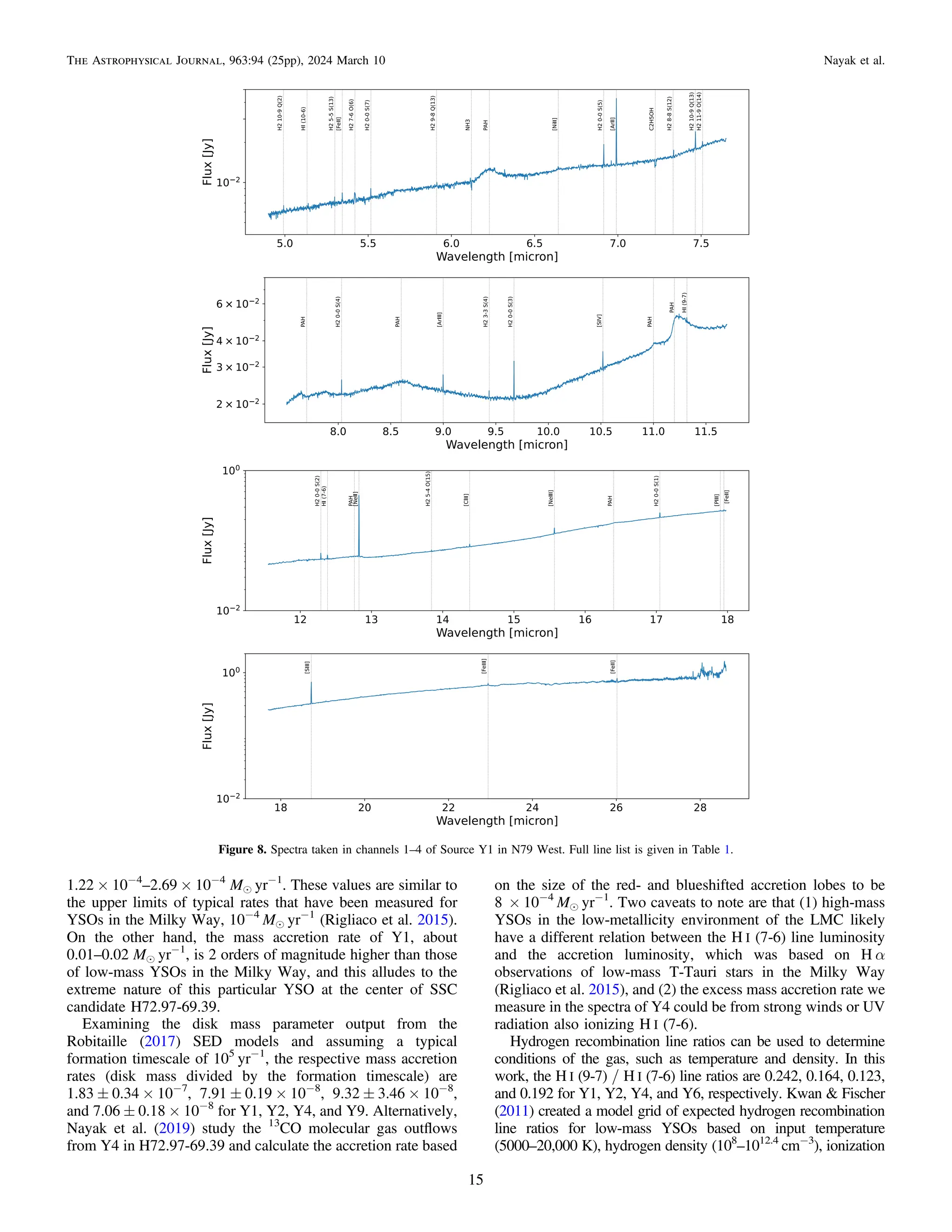
The MRS spectra of Y1, Y2, Y3, Y4, Y6, and Y9 all show
increasing flux toward mid-IR wavelengths, a characteristic
typical of YSOs (Figure 2). Additionally, we see broad
absorption lines, broad PAH emission lines, and narrow
emission lines. The long-wavelength MRS subband 4C has a
lower signal-to-noise (S/N) ratio, making line fitting from
wavelengths 24.4 to 28.6 μm less reliable. Even in subbands
1A through 4B, the fluxes extracted from Gaussian fitting are
dependent upon determining emission- and absorption-free
ranges for continuum fitting and subtraction. Modeling the
emission lines with CLOUDY and PAHFIT will be done in a
later paper. In this work, we discuss the details of the various
Table 5
Source Y6 Emission and Absorption Lines
Name Absorption or Lab Wave Meas Wave Meas Wave Err FWHM Flux Flux Err
Emission (μm) (μm) (μm) (μm) (erg s−1
cm−2
) (erg s−1
cm−2
)
H2 9-8 Q(13) E 5.909 5.91289 0.00031 0.00209 1.237E-15 5.581E-17
PAH E 6.200 6.23934 0.00168 0.12349 4.838E-14 2.093E-15
H2 2-1 O(12) E 6.776 6.77683 0.00077 0.00248 4.536E-16 3.956E-17
H2 0-0 S(5) E 6.910 6.91559 0.00039 0.00177 1.119E-15 4.166E-17
[Ar II] 2P1/2-2P3/2 E 6.985 6.99106 0.00014 0.00147 2.919E-14 6.152E-16
H2 11-9 O(14) E 7.506 7.50930 0.00050 0.00233 3.471E-15 1.009E-16
[Ni I] a3F3-a3F4 E 7.507 7.51107 0.00333 0.00104 1.122E-15 6.581E-17
PAH E 7.700 7.63727 0.03884 0.40222 1.327E-13 4.066E-14
H2 0-0 S(4) E 8.025 8.03162 0.00033 0.00271 8.518E-16 1.387E-16
H I (10-7) E 8.760 8.76730 0.00045 0.00278 7.269E-16 1.397E-16
[Ar III] 3P1-3P2 E 8.991 8.99845 0.00020 0.00314 2.073E-14 5.794E-16
H2 0-0 S(3) E 9.665 9.67272 0.00023 0.00250 1.877E-15 1.568E-16
[S IV] 2P3/2-2P1/2 E 10.511 10.51874 0.00021 0.00290 1.274E-14 3.472E-16
PAH E 11.200 11.26670 0.00103 0.16708 1.134E-13 2.218E-15
H I (9-7) E 11.310 11.31777 0.00062 0.00322 1.940E-15 1.868E-16
H2 0-0 S(2) E 12.279 12.28880 0.00005 0.00400 2.890E-15 4.229E-16
H I (7-6) E 12.370 12.38179 0.00054 0.00468 1.013E-14 7.068E-16
H I (11-8) E 12.387 12.39659 0.00034 0.00643 1.941E-15 4.093E-16
[Ne II] 2P1/2-2P3/2 E 12.814 12.82418 0.00043 0.00411 2.285E-13 4.481E-15
HCN A 14.050 13.97779 0.00044 0.00806 1.757E-15 3.056E-16
[Cl II] 3P1-3P2 E 14.368 14.37792 0.00083 0.00459 1.223E-15 4.779E-16
[Ne III] 3P1-3P2 E 15.555 15.56774 0.00101 0.00652 1.422E-13 1.609E-15
H I (10-8) E 16.209 16.22067 0.00058 0.00703 1.552E-15 6.704E-16
H2 0-0 S(1) E 17.035 17.04911 0.00036 0.00524 5.884E-15 7.255E-16
[P III] 2P3/2-2P1/2, E 17.885 17.89809 0.00066 0.00781 1.078E-15 7.461E-16
[Fe II] a4F7/2-a4F9/2 E 17.936 17.94888 0.00125 0.00725 2.028E-15 1.110E-15
[S III] 3P2-3P1 E 18.713 18.72739 0.00161 0.00939 2.311E-13 8.686E-15
H I (8-7) E 19.062 19.07710 0.00010 0.00786 3.549E-15 5.163E-15
[Ar III] 3P0-3P1 E 21.830 21.84428 0.00072 0.00761 7.731E-15 5.142E-15
[Fe III] 5D3-5D4 E 22.925 22.94357 0.00056 0.00943 5.923E-15 5.517E-15
[Fe II] a6D7/2-a6D9/2 E 25.998 26.01276 0.05576 0.02060 5.419E-14 4.615E-13
Notes. Column (1): Name of line. Column (2): Emission or absorption line. “E” stands for emission, and “A” stands for absorption. Column (3): Laboratory
wavelength. Column (4): Measured wavelength. Column (5): Error in measured wavelength. Column (6): FWHM of line. Column (7): Measured flux. Column (8):
Error in flux.
8
The Astrophysical Journal, 963:94 (25pp), 2024 March 10 Nayak et al.](https://image.slidesharecdn.com/nayak2024apj96394-250127005706-08738261/75/JWST-Mid-infrared-Spectroscopy-Resolves-Gas-Dust-and-Ice-in-Young-Stellar-Objects-in-the-Large-Magellanic-Cloud-8-2048.jpg)
![emission and absorption lines of six out of the 11 total YSOs
from the N79 region of the LMC shown in Figures 8–13 and
reported in Tables 1–6. The five other YSOs in this sample
have partial spectra. Additionally, the few emission lines they
have are similar to one of the YSOs with a full MRS spectrum,
implying these are not the dominating source within the cluster.
5.1. PAH Emission
PAHs are essential to the balance between photoionization
and recombination rates. Mid-IR observations of dusty sources
(e.g., YSOs, H II regions, planetary nebulae, reflection nebulae,
and asymptotic giant branch stars) often show PAH emission
at 6.2, 7.7, 8.6, 11.2, 12.7, and 16.4 μm (Hony et al. 2001;
Peeters et al. 2002; Shannon et al. 2016). The PAH features in
the 5–10 μm region originate from the pure CC stretching
mode as well as the CH in-plane bending mode (Joblin et al.
1996; Hony et al. 2001). The 10–15 μm PAH features are due
to the out-of-plane bending vibrations of aromatic H atoms
(Hony et al. 2001). The 7.7 μm emission feature originates
from positively charged grains, whereas the 11.2 μm emission
is from neutral grains (Hony et al. 2001). The PAH11.2/PAH7.7
ratio is sensitive to the fraction of ionized to neutral PAHs
(Draine & Li 2001). The 15–20 μm region is because of the
CCC modes of PAHs (Smith et al. 2007). In addition to the
above six PAH emission lines, we also observe the faint and
positively charged 11 μm feature for three YSOs in N79.
Table 6
Source Y9 Emission and Absorption Lines
Name Absorption or Lab Wave Meas Wave Meas Wave Err FWHM Flux Flux Err
Emission (μm) (μm) (μm) (μm) (erg s−1
cm−2
) (erg s−1
cm−2
)
[Fe II] a4F9/2-a6D9/2 E 5.340 5.34445 0.00007 0.00163 4.549E-16 6.039E-17
H2 2-1 O(10) E 5.409 5.40474 0.00114 0.00094 8.026E-17 6.885E-18
H2 0-0 S(7) E 5.511 5.51611 0.00168 0.12349 4.838E-14 2.093E-15
H2 0-0 S(6) E 6.109 6.11485 0.00077 0.00248 4.536E-16 3.956E-17
PAH E 6.200 6.22564 0.00046 0.10209 3.688E-14 5.239E-16
H2 0-0 S(5) E 6.910 6.91506 0.00039 0.00177 1.119E-15 4.166E-17
[Ar II] 2P1/2-2P3/2 E 6.985 6.99097 0.00014 0.00147 2.919E-14 6.152E-16
H2 10-9 Q(13) E 7.452 7.46467 0.00173 0.00206 1.097E-16 2.175E-17
PAH E 7.700 7.71042 0.00167 0.42496 1.743E-13 2.186E-15
H2 0-0 S(4) E 8.025 8.03178 0.00050 0.00233 3.471E-15 1.009E-16
PAH E 8.600 8.60527 0.00469 0.25788 4.374E-14 2.523E-15
H2 0-0 S(3) E 9.665 9.67303 0.00333 0.00104 1.122E-15 6.581E-17
PAH E 11.000 11.01046 0.01876 0.05358 3.006E-15 3.343E-15
PAH E 11.200 11.25369 0.00079 0.13108 5.634E-14 1.079E-15
H2 0-0 S(2) E 12.279 12.28889 0.03883 0.40231 1.327E-13 4.065E-14
H I (7-6) E 12.370 12.38211 0.00033 0.00271 8.518E-16 1.387E-16
PAH E 12.700 12.76987 0.00636 0.22928 3.827E-14 3.371E-15
[Ne II] 2P1/2-2P3/2 E 12.814 12.82475 0.00020 0.00314 2.073E-14 5.794E-16
[Cl II] 3P1-3P2 E 14.368 14.37866 0.00023 0.00250 1.877E-15 1.568E-16
CO2 A 14.970 14.99625 0.00070 0.00829 2.811E-16 7.555E-17
CO2 A 15.200 15.26561 0.00195 0.03826 1.150E-15 1.866E-16
PAH E 16.400 16.44424 0.00113 0.14098 1.159E-14 2.950E-16
H2 0-0 S(1) E 17.035 17.04970 0.00095 0.00603 4.074E-15 1.134E-16
[Fe II] a4F7/2-a4F9/2 E 17.936 17.94714 0.00110 0.00915 6.789E-16 2.811E-16
[S III] 3P2-3P1 E 18.713 18.72798 0.00021 0.00290 1.274E-14 3.472E-16
[Fe II] a6D7/2-a6D9/2 E 25.998 26.01709 0.04723 0.00944 4.592E-15 5.425E-14
Notes. Column (1): Name of line. Column (2): Emission or absorption line. “E” stands for emission, and “A” stands for absorption. Column (3): Laboratory
wavelength. Column (4): Measured wavelength. Column (5): Error in measured wavelength. Column (6): FWHM of line. Column (7): Measured flux. Column (8):
Error in flux.
Table 7
Summary of Emission and Absorption Lines Observed in YSOs
Name 6.2 μm 7.7 μm 8.6 μm 11.0 μm 11.2 μm 12.7 μm 16.4 μm
CO2
Absorp. No. of Other No. of No. of No. of
PAH PAH PAH PAH PAH PAH PAH Line
Absorp.
Lines H I Lines
Fine-structure
Lines H2 Lines
Y1 ✓ ✓ ✓ ✓ ✓ ✓ ✓ 2 2 13 15
Y2 ✓ ✓ ✓ ✓ ✓ ✓ ✓ 0 9 13 16
Y3 ✓ ✓ 4 1 3 5
Y4 1 8 11 15
Y6 ✓ ✓ ✓ 1 6 13 8
Y9 ✓ ✓ ✓ ✓ ✓ ✓ ✓ ✓ 1 1 7 9
9
The Astrophysical Journal, 963:94 (25pp), 2024 March 10 Nayak et al.](https://image.slidesharecdn.com/nayak2024apj96394-250127005706-08738261/75/JWST-Mid-infrared-Spectroscopy-Resolves-Gas-Dust-and-Ice-in-Young-Stellar-Objects-in-the-Large-Magellanic-Cloud-9-2048.jpg)
![The 6.2 μm PAH feature is seen in the spectra of Y1 located
in W1, Y2 located in E1, Y6 located in SSC region S1, and Y9
located in S2. The 6.2 μm emissions for sources Y6 and Y9
have red tails, which can be seen in Figures 12 and 13. The
peak position of the 6.2 μm PAH feature for Y6 is 6.239 μm,
whereas for the other three sources the peak position ranges
from 6.225 to 6.227 μm, slightly shorter in wavelength.
Additionally, source Y6 has an FWHM of 0.123 μm, larger
than the FWHM of the 6.2 μm for Y1, Y2, and Y9 by 20%.
Peeters et al. (2002) observe a similar asymmetric red tail and
larger FWHM for the PAH emissions whose peak positions are
greater than 6.23 μm for 57 different dusty sources, including
YSOs, planetary nebulae, and other galaxies. They attribute the
observed asymmetry in the 6.2 μm emission line to a
combination of PAH stretching and bending modes, one with
emission at 6.2 μm and another with emission at 6.3 μm.
The 7.7 μm PAH feature is seen as a double emission line for
sources Y1 and Y2, where there is a peak around 7.6 μm,
arising from small grains, and another peak around 7.8 μm,
arising from large grains. The 7.6 μm feature is the dominant
emission, with a flux 10% greater than the 7.8 μm feature in Y1
and 40% greater than the 7.8 μm feature in Y2. Sources Y6 and
Y9 also emit the 7.7 μm PAH feature; however, there is no
secondary emission around 7.8 μm.
The 8.6 μm and much weaker 11.0 μm PAH emission lines
are present in Y1, Y2, and Y9. The 8.6 μm line is 63, 13, and
15 times stronger than the 11.0 μm line for sources Y1, Y2, and
Y9, respectively. The charged state of the ionized PAHs that
emit in the 5–10 μm region also lead to the 11.0 μm emission
(Hudgins et al. 2004). Peeters et al. (2017) find a correlation
between the 8.6 and 11.0 μm emission. Their observations
show that the 8.6 μm emission from the CH in-plane bending
mode and the 11.0 μm emission from the out-of-plane bending
mode of the H atom are closer to the central illuminating source
NGC 2023. There also is a close correlation between the 7.6
and 11.0 μm PAHs (Peeters et al. 2017). We find that YSOs
with both the 8.6 and 11.0 μm emission lines also have 7.7 μm
emission, indicating a correlation of similar origin for the three
different PAH emission lines.
Every YSO, except for Y4 located in the central ionizing
source in H72.97-69.39, exhibits the 11.2 μm PAH emission
line. Y1, Y2, and Y9 have the 12.7 and 16.4 μm PAH features.
Further away from the central ionizing source are the PAHs
that give rise to the 7.7 μm emission line, more specifically the
large grains that emit at 7.8 μm (Bauschlicher & Peeters 2008).
With increasing proximity to the central ionizing source, these
PAHs that emit at 7.8 μm break down into smaller grains,
leading to the 11.2 μm emission. These PAHs are further
broken down closer to the central ionizing source and emit at
12.7 and 16.4 μm. The 6.2, small grain 7.7, 8.6, and 11 μm
PAH emission features occur closest to the central YSO.
Both shocks and UV radiation can enhance certain
PAH emission lines by dissociating large grains, but they
can also destroy the PAH molecules (Hony et al. 2001;
Figure 3. Slices of the IFU cube in N79W: The H2 0-0 S7 emission at 5.51 μm (top left), PAH emission at 6.2 μm (top center), PAH emission at 11.2 μm (top right),
[Ne II] emission at 12.81 μm (bottom left), H2 0-0 S1 emission at 17.04 μm (bottom center), and [S III] emission at 18.71 μm (bottom right). We label this single YSO
as “Y1” in the bottom right panel. The contour levels for H2 emission at 5.51 μm, PAH emission at 6.2 μm, PAH emission at 11.2 μm, and [Ne II] emission at
12.81 μm are 500, 2500, and 4500 MJy sr−1
. The contour levels for H2 emission at 17.04 μm and [S III] emission at 18.71 μm are 2500, 5000, and 10,000 MJy sr−1
.
10
The Astrophysical Journal, 963:94 (25pp), 2024 March 10 Nayak et al.](https://image.slidesharecdn.com/nayak2024apj96394-250127005706-08738261/75/JWST-Mid-infrared-Spectroscopy-Resolves-Gas-Dust-and-Ice-in-Young-Stellar-Objects-in-the-Large-Magellanic-Cloud-10-2048.jpg)
![O’Halloran et al. 2006). The mass of cluster S1 (including source
Y4) is 25.4 Me, and the luminosity is 1.2 × 10⁵
Le. This cluster
is an order of magnitude more luminous than the other clusters in
this work, with Y4 most likely dominating the SED. Y4 has no
PAH emission lines, because of the intense ionizing radiation of
this YSO destroying PAH molecules.
5.2. Molecular Hydrogen Lines
H2 emission can be the result of shock heating of the
molecular gas by outflows from the central protostar, or UV
heating of nearby gas to a few hundred degrees Kelvin by the
massive star. We find several H2 rotational lines in Y1, Y2, Y3,
Y4, Y6, and Y9. The three H2 emission lines common to all six
YSOs in this work are the H2 0-0 S4 line at 8.03 μm, H2 0-0 S3
line at 9.67 μm, and H2 0-0 S1 line at 17.03 μm. We show the
IFU slices at 5.51 μm (H2 0-0 S7) and 17.03 μm in
Figures 3–6. The 17.03 μm emission is stronger than that at
5.51 μm, indicating that these are young and deeply embedded
YSOs with a steep rise in their SED toward mid-IR and far-IR
wavelengths. Furthermore, the longer-wavelength slices reveal
additional embedded YSOs. This is especially noticeable for
region S1, shown in Figure 5, where the 5.51 μm slice has two
YSOs, whereas there are five YSOs in the 17.03 μm slice.
Previous observations of the reflection nebula NGC 2023 and
the Orion Bar have shown the H2 emission to trace PDR fronts
(Peeters et al. 2017; Knight et al. 2021). Future analysis will
use PAHFIT and CLOUDY modeling to derive gas properties
based on the PAH emission lines and narrow fine-structure
emission lines. Properties such as extinction, shock excitation,
temperature, density, and wind velocity will be calculated using
line ratios (Morisset et al. 2002, 2004; Simpson et al. 2012;
Stock et al. 2013; Lambert-Huyghe et al. 2022).
5.3. Fine-structure Emission
Fine-structure emission is often seen in YSOs that also
exhibit PAH emission, indicating that the central illuminating
source is emitting UV radiation. Neon, sulfur, and argon lines
have previously been observed in W1, E1, S1, and S2 with
Spitzer IRS (Seale et al. 2009). In PDRs, the UV photons from
the central star are ionizing atomic species with ionization
potential 13.6 eV and below, (i.e., [Fe I], [Fe II], [Si I]). Shocks
from winds and jets can heat up the gas to 105
K (Draine &
McKee 1993; Hollenbach 1997). These strong shocks with
velocities greater than 70 km s−1
result in [Ni II] 6.6, [Ar II] 6.9,
[Ne II] 12.8, [Ar III] 8.9 and 21.8, and [Fe II] 26 μm emission
lines, which need high ionization energy (> 21 eV).
5.3.1. Neon Fine-structure Line Emission
The presence of [Ne II] and [Ne III], which requires
ionization energy > 41 eV, means there are high-energy UV
Figure 4. Slices of the IFU cube in N79E: The H2 0-0 S7 emission at 5.51 μm (top left), PAH emission at 6.2 μm (top center), PAH emission at 11.2 μm (top right),
[Ne II] emission at 12.81 μm (bottom left), H2 0-0 S1 emission at 17.04 μm (bottom center), and [S III] emission at 18.71 μm (bottom right). We label the two sources
within the MRS FOV as “Y2” and “Y3” in the bottom right panel. The contour levels for H2 emission at 5.51 μm, PAH emission at 6.2 μm, PAH emission at 11.2 μm,
and [Ne II] emission at 12.81 μm are 600, 2000, and 4500 MJy sr−1
. The contour levels for H2 emission at 17.04 μm and [S III] emission at 18.71 μm are 3000, 6000,
and 12,000 MJy sr−1
.
11
The Astrophysical Journal, 963:94 (25pp), 2024 March 10 Nayak et al.](https://image.slidesharecdn.com/nayak2024apj96394-250127005706-08738261/75/JWST-Mid-infrared-Spectroscopy-Resolves-Gas-Dust-and-Ice-in-Young-Stellar-Objects-in-the-Large-Magellanic-Cloud-11-2048.jpg)
![photons either from the central star or high-velocity shocks.
YSOs Y1, Y2, Y3, Y4, and Y6 have both the [Ne II] 12.8 μm
and [Ne III] 15.5 μm lines. YSO Y9 only has the [Ne II]
12.8 μm line. The [Ne II] / H2 S(1) ratios (often used to infer
shock velocity) for sources Y1, Y2, Y3, Y4, Y6, and Y9 are
15.4, 38.9, 0.5, 97.4, 38.8, and 5.1, respectively. We use the
Hollenbach et al. (1989) shock models of high-velocity
(v = 40–150 km s−1
) jump shocks where gas is heated to
temperatures as high as 105
K in a timescale shorter than
the characteristic cooling time. At low densities (n = 103
–
105
cm−3
), hydrogen recombination lines, [Fe II] 5.3 μm,
[Ne II] 12.8 μm, and [Fe II] 26.3 μm are predicted from the
models. When densities are n = 105
–107
cm−3
, there is an
increase in [Cl I] 11.3 μm, and [Fe I] 24 μm. Assuming a
molecular gas density of n = 104
–105
cm−3
and using the
Hollenbach et al. (1989) shock models, the shock velocities
associated with the [Ne II] emission are 140, 120, 50, 100, 120,
and 90 km s−1
for Y1, Y2, Y3, Y4, Y6, and Y9, respectively. A
more detailed constraint using multiple fine-structure line ratios
will be presented in a later paper.
For shock velocities 30–40 km s−1
, Hollenbach et al. (1989)
predict H2 S(1), H2 S(2), H2 S(3), as well as the [Fe II] 26 μm to
be stronger than the [Ne II] line by 1–3 orders of magnitude.
However, we observe the [Ne II] line to be stronger in every
source except for Y3, implying shock velocities >70 km s−1
(Hollenbach et al. 1989). Y3 is the youngest protostar in this
study, with deep absorption lines implying this source is
younger than 10,000 yr old. The lack of multiple different
ionization lines and the low shock velocity inferred from the
Hollenbach et al. (1989) models suggests that Y3 is still very
embedded: The UV radiation from the central star has not yet
begun to ionize the surrounding gas, and the accretion rate is
lower in comparison to the other five YSOs in this work.
Hollenbach & Gorti (2009) find shocks from protostellar winds
can explain the observed [Ne II] emission, especially when the
mass accretion rate (which is proportional to the protostellar
wind mass-loss rate) is higher than 10−8
Me yr−1
. However,
they also find that low-mass protostars with low accretion rates
are associated with [Ne II], due to UV and X-ray radiation from
nearby high-mass stars photoexciting the gas (Hollenbach &
Gorti 2009).
5.3.2. Sulfur and Iron Lines in Spectra of Protostars
If high shock velocities are the origin of the observed line
emission, the [Fe I] line at 24 μm and [S I] line at 25.3 μm
should be detected, with the [S I] line being the stronger of the
two (Hollenbach et al. 1989). With low-velocity shocks, H2
emission is particularly strong and atomic lines are expected to
be weak (Kaufman & Neufeld 1996). The YSOs in this work
likely have a mix of high- and low-velocity shocks, as we
Figure 5. Slices of the IFU cube in N79S1: The H2 emission at 5.51 0-0 S7 μm (top left), PAH emission at 6.2 μm (top center), PAH emission at 11.2 μm (top right),
[Ne II] emission at 12.81 μm (bottom left), H2 0-0 S1 emission at 17.04 μm (bottom center), and [S III] emission at 18.71 μm (bottom right). We label the five sources
within the MRS FOV as “Y4,” “Y5,” “Y6,” “Y7,” and “Y8” in the bottom right panel. The contour levels for H2 emission at 5.51 μm are 2000, 10,000, and
35,000 MJy sr−1
. The contour levels for PAH emission at 6.2 μm are 4000, 10,000, 35,000 MJy sr−1
. The contour levels for PAH emission at 11.2 μm and [Ne II]
emission at 12.81 μm are 5000, 15,000, and 45,000 MJy sr−1
. The contour levels for H2 emission at 17.04 μm are 9000, 20,000, and 55,000 MJy sr−1
. The contour
levels for [S III] emission at 18.71 μm are 35,000, 80,000, and 230,000 MJy sr−1
.
12
The Astrophysical Journal, 963:94 (25pp), 2024 March 10 Nayak et al.](https://image.slidesharecdn.com/nayak2024apj96394-250127005706-08738261/75/JWST-Mid-infrared-Spectroscopy-Resolves-Gas-Dust-and-Ice-in-Young-Stellar-Objects-in-the-Large-Magellanic-Cloud-12-2048.jpg)
![observe strong fine-structure atomic lines as well as multiple
H2 lines. [S I], [Fe I], and [Fe II] lines can be used to determine
if slow- or fast-velocity shocks are dominating the region
(Hollenbach et al. 1989).
5.3.3. Detection of [Cl II]
The [Cl II] fine-structure emission line at 14.37 μm is
observed for sources Y1, Y2, Y4, Y6, and Y9. The respective
offset velocities of the [Cl II] line are 7.9, 4.5, 13.4, 26.4, and
10.9 km s−1
for sources Y1, Y2, Y4, Y6, and Y9. The [Cl II]
line has an ionized potential of 13 eV and could originate from
shocks where the ionized gas is heated up to 105
K (Hollenbach
et al. 1989). Collimated jets associated with Herbig–Haro (HH)
objects HH529 and HH204 have been observed in the Orion
Nebula (Méndez-Delgado et al. 2021a, 2021b). Line emissions
from [Cl II], [Cl III], and [Cl IV] have been observed with both
HH sources, with velocity offsets ranging from 11 to 36 km s−1
(Méndez-Delgado et al. 2021a, 2021b), similar to the velocity
offset we observe with the [Cl II] emission line associated with
YSOs in N79. Low-velocity jets and bow shocks < 30 km s−1
could be one possible origin for the observed [Cl II] in
N79 YSOs.
5.4. H I Emission Line
MRS observations reveal, for the first time, several mid-IR
hydrogen recombination lines in the spectra of extragalactic
YSOs in N79. Hydrogen recombination lines can be used to
estimate the accretion rate. Alcalá et al. (2014) used the Very
Large Telescope (VLT) X-shooter to observe the Brackett,
Balmer, and Paschen hydrogen recombination lines, to derive
accretion rates of 2 × 10⁻¹²
–2 × 10⁻⁸
Me yr−1
for low-mass
YSOs in the mass range 0.3–1.2 Me. Deeply embedded sources
like the YSOs in this work require detection of mid-IR
hydrogen recombination lines. We find Y1, Y2, Y4, and Y6 to
have both H I (9-7) emission at 11.31 μm and Humphreys α H I
(7-6) emission at 12.37 μm. Y9 has only the H I (7-6) emission.
Rigliaco et al. (2015) used Spitzer IRS observations of 114
T-tauri stars with disks to find a correlation between the H I (7-
6) emission and the accretion luminosity:
( ) ( )
( )
( )
L
L
L
L
log 0.48 0.09 log 4.68 0.10 .
1
HI 7 6 acc
= ´ -
-
The factor of 0.48 from Rigliaco et al. (2015) sets a nearly
quadratic dependence between the line and accretion luminos-
ity. This strong dependence is at odds with the nearly linear
Figure 6. Slices of the IFU cube in N79S2: The H2 0-0 S7 emission at 5.51 μm (top left), PAH emission at 6.2 μm (top center), PAH emission at 11.2 μm (top right),
[Ne II] emission at 12.81 μm (bottom left), H2 0-0 S1 emission at 17.04 μm (bottom center), and [S III] emission at 18.71 μm (bottom right). We label the three
sources within the MRS FOV as “Y9,” “Y10,” and “Y11” in the bottom right panel. The contour levels for H2 emission at 5.51 μm are 500, 1000, and 8000 MJy sr−1
.
The contour levels for the PAH emission at 6.2 μm are 500, 1000, and 4000 MJy sr−1
. The contour levels for the PAH emission at 11.2 μm are 700, 1000, and
3000 MJy sr−1
. The contour levels for the [Ne II] emission at 12.81 μm are 600, 1000, and 4000 MJy sr−1
. The contour levels for H2 emission at 17.04 μm are 1500,
4000, and 15,000 MJy sr−1
. The contour levels for the [S III] emission at 18.71 μm are 1000, 4000, and 15,000 MJy sr−1
.
13
The Astrophysical Journal, 963:94 (25pp), 2024 March 10 Nayak et al.](https://image.slidesharecdn.com/nayak2024apj96394-250127005706-08738261/75/JWST-Mid-infrared-Spectroscopy-Resolves-Gas-Dust-and-Ice-in-Young-Stellar-Objects-in-the-Large-Magellanic-Cloud-13-2048.jpg)
![rate, and velocity gradient transverse to the radial direction
(the ratio of the turbulent/thermal line width). Their predicted
H I (9-7) / H I (7-6) line ratios ranged from 0.3–2.1, higher than
the observed line ratios in this work, which range from 0.12–0.24.
An increase in dl/dv, the ratio of the turbulent/thermal line width,
leads to an increase in the line optical depth, τ (Equation (1) in
Kwan & Fischer 2011), which is one of the parameters in their
modelings. Kwan & Fischer (2011) assume the velocity gradient
dl/dv is not large and the model results do not vary much on the
gradient. Massive stars whose turbulent velocities from winds and
radiation are greater than those of low-mass stars would have very
different dl/dv than what was modeled, and therefore could be the
reason we find the H I (9-7) / H I (7-6) line ratios to be smaller
than the predicted ratios from Kwan & Fischer (2011).
Hollenbach & Gorti (2009) find the ratio of H I (7-6) to the
[Ne II] fine-structure line to theoretically be 0.008, due to
extreme UV- and X-ray-illuminated shocks. The observed
ratios in this work range from 0.11 for Y4 to 0.04 for Y1, Y2,
Y5, and Y6. The observed ratios are higher than the theoretical
ratios, which means the origin of the hydrogen recombination
line must be from regions where the density is higher than the
critical density of [Ne II]. Hollenbach & Gorti (2009) suggest
an alternate scenario where the observed H I lines in high-mass
protostars in N79 could arise from shocks due to high-velocity
winds. Hollenbach & Gorti (2009) find winds with velocities
> 100 km s−1
that occur close to the origin of the central source
(< 1 au), leading to densities where H I (7-6) emission is
enhanced but the [Ne II] emission is suppressed. This excess H I
Figure 9. Spectra taken in channels 1–4 of Source Y2 in N79 East. Full line list is given in Table 2.
16
The Astrophysical Journal, 963:94 (25pp), 2024 March 10 Nayak et al.](https://image.slidesharecdn.com/nayak2024apj96394-250127005706-08738261/75/JWST-Mid-infrared-Spectroscopy-Resolves-Gas-Dust-and-Ice-in-Young-Stellar-Objects-in-the-Large-Magellanic-Cloud-16-2048.jpg)
![(7-6) emission would also explain the high mass accretion rates
calculated, as the measured emission would be from shocks and
winds in addition to accretion. Massive YSOs have previously
been observed to have high-velocity winds: S106-IR has an
ionized wind with a velocity of 340 km s−1
(Drew et al. 1993),
and W51 IRS2 is a 60 Me O star with a 200 Me molecular
outflow and wind velocities of 100 km s−1
inferred from the
[Ne II] emission line (Lacy et al. 2007; Zapata et al. 2009).
Given that these YSOs in N79 are very massive (11–25 Me)
and extremely luminous (6.8 × 10³
–1.3 × 10⁵
Le), outflows
with velocities > 100 km s−1
are a likely scenario. Such
conditions in N79 would explain why the observed H I (7-6)
to [Ne II] ratio is higher than theoretical models.
5.4.1. The Central Illuminating Source Y4 in H72.97-69.39
MRS observations of H72.97-69.39 show five sources
within the FOV (Figure 5). Figure 2 shows the spectra of
Y5, Y7, and Y8, which are not complete, but they still show
similar emission line features to Y4 and Y6 in channels 3 and
4. The Spitzer IRS spectrum of S1, shown in red in Figure 2,
resembles the MRS spectrum of Y4. This is the more luminous
source and is likely dominating the SED of the small cluster,
with Y6 as the second-most dominant source. ALMA
observations of H72.97-69.39 reveal two filaments colliding,
with Y4 located in the center (Nayak et al. 2019). Figure 14
shows the blue- and redshifted outflows observed with 13
CO on
the MRS channel 3 slice of H72.97-69.39. Nayak et al. (2019)
find an outflow rate of 0.008 Me yr−1
associated with the
central protostar inferred from the redshifted outflow lobe, four
times higher than outflow rates of massive YSOs in the Milky
Way (Beltrán et al. 2011). Commonly found to trace hot
molecular cores and the cavity of outflowing jets, SO is a useful
diagnostic of shocked gas (Esplugues et al. 2013; Codella et al.
2014). ALMA SO observations trace gas densities of 106
cm−3
,
which are offset from the outflow axis by 90°. Further ALMA
observations with spectral resolution higher than that used by
Nayak et al. (2019) will be necessary to determine the
kinematic structure of SO. It is possible the high-velocity winds
> 100 km s−1
that cause the hydrogen recombination line H I
(7-6) emission also lead to the observed SO emission. The wind
could be compressing the gas to 106
cm−3
in the immediate
vicinity of Y4, leading to a lower [Ne II] emission, higher H I
(7-6) emission, and the observed SO emission (Hollenbach &
Gorti 2009; Nayak et al. 2019).
Reiter et al. (2019) use the Folded-Port Infrared Echellette
(FIRE; Simcoe et al. 2013) on the 6.5 m Magellan/Baade
telescope to observe the near-IR spectrum of H72.97-69.39
(with Y4 likely being the dominating YSO). They find the
H2/Brγ ratio (i.e., the ratio of collisionally excited to
photoexcited gas) is 0.01. Additionally, Reiter et al. (2019)
find the region around H72.97-69.39 is likely not shock-
excited, based on the low [Fe II] 1.64 μm/Paβ and [Fe II]
1.64 μm/Brγ ratios of 0.02 and 0.11, respectively. Both Brγ
Figure 10. Spectra taken in channels 2–4 of Source Y3 in N79 East. Full line list is given in Table 3.
17
The Astrophysical Journal, 963:94 (25pp), 2024 March 10 Nayak et al.](https://image.slidesharecdn.com/nayak2024apj96394-250127005706-08738261/75/JWST-Mid-infrared-Spectroscopy-Resolves-Gas-Dust-and-Ice-in-Young-Stellar-Objects-in-the-Large-Magellanic-Cloud-17-2048.jpg)
![Figure 14. Left: The [Ne II] line emission slice overlaid with the ALMA 13
CO blueshifted (cyan contour) and redshifted (red contour) outflows. The outflows were
determined by Nayak et al. (2019) by integrating over the line wings of the 13
CO spectrum. Right: The ALMA SO observations (magenta contour) shown with the
MRS [Ne II] line emission slice.
Figure 15. Top Left: The 13.8–16.2 μm MRS spectrum of Y3 and the locally fitted continuum. Top Right: The continuum-subtracted spectrum of the CO2 absorption
feature. Bottom: We fit two and three Gaussian distributions to the CO2 mixture feature. The residual error when fitting three Gaussian distributions is 0.41 and the
residual error when fitting two Gaussian distributions is 0.53; therefore, the three Gaussians give a better fit to the observed absorption line. The two peaks at 15.1 and
15.3 μm represent a CO2-CO and a CO2-H2O mixture, respectively. The broad shoulder at longer wavelengths is due to a mixture of CO2-CH3OH.
21
The Astrophysical Journal, 963:94 (25pp), 2024 March 10 Nayak et al.](https://image.slidesharecdn.com/nayak2024apj96394-250127005706-08738261/75/JWST-Mid-infrared-Spectroscopy-Resolves-Gas-Dust-and-Ice-in-Young-Stellar-Objects-in-the-Large-Magellanic-Cloud-21-2048.jpg)
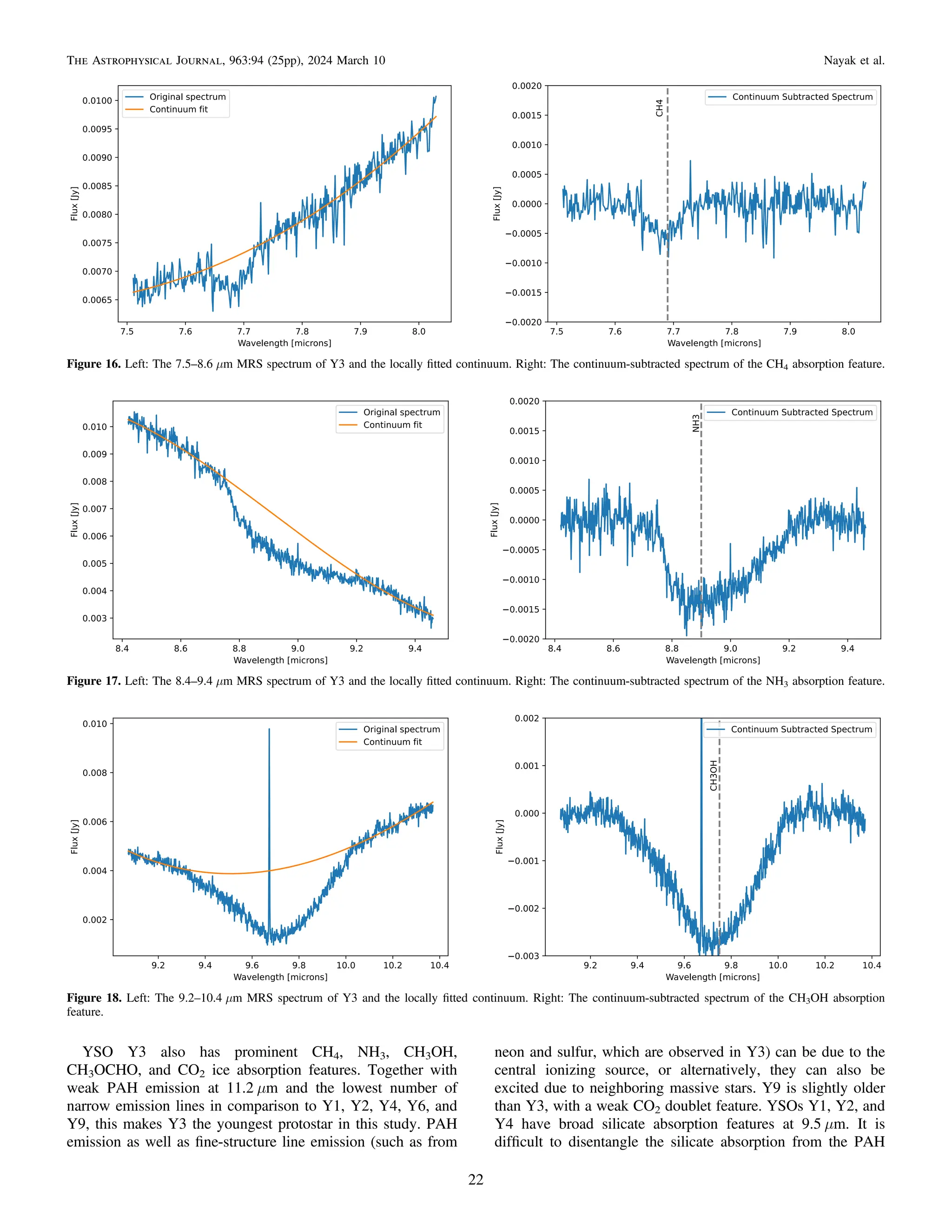
![emission at 8.5 μm and 11 μm without modeling, which will be
done in a later paper. The silicate absorption along with several
H2 and fine-structure line emissions, coupled with the lack of
any other broad ice absorption in these three YSOs, suggests
these are more evolved YSOs, with UV radiation from the
central star affecting their parental molecular gas. Y6 is the
oldest YSO in this work, because this source has no silicate or
ice absorption features.
6. Summary
We present MIRI MRS observations of 11 YSOs in the N79
region of the LMC, six of which have a full or almost-full
wavelength coverage from 4.9 to 27.9 μm. The blended
Spitzer-identified YSOs are resolved into multiple protostars
in the MRS IFU observations in N79 East and South. The
Spitzer-identified YSO in N79 West is a single massive source.
We identify the mid-IR emission and absorption lines for the
six YSOs in Tables 1–6 and summarize our findings:
1. The respective masses inferred by fitting SED models to
the Spitzer and Herschel photometry for clusters E1, S1, and S2
are 18.3 ± 2.7, 25.4 ± 3.2, and 15.7 ± 4.5 Me. Y2 is likely the
dominating source in E1, Y4 is the dominating source in S1,
and Y9 is the dominating source in S2. The isolated massive
protostar Y1 in W1 has a mass of 13.6 ± 1.6 Me.
2. The YSOs have a variety of PAH emission lines at 6.2,
7.7, 8.6, 11.0, 11.2, 12.7, and 16.4 μm. YSOs Y1, Y2, and Y9
have all seven PAH emission features in their spectra. Y6 has
the 6.2, 7.7, and 11.2 μm PAH emission features, and Y3 only
has 11.2 μm emission. YSO Y4, the central ionizing source of
SSC candidate H72.97-69.39, has no PAH features, likely due
to the intense radiation and strong stellar winds destroying the
surrounding PAHs.
3. All six YSOs have several molecular hydrogen emission
lines. Y2 located in the East GMC has 16 H2 lines, the greatest
number of emission lines out of all the sources in this work.
Y3, the youngest source, has five H2 lines. The prominent
absorption lines seen in the spectrum of Y3 indicate that this
protostar is enshrouded by dust and the central protostar has not
started ionizing the surrounding gas. The H2 lines seen in the
spectra of Y3 could be due to the dominant source, Y2,
exciting the H2.
4. [Ne II] 12.8 μm, [Ne III] 15.5 μm, [Ar II] 6.9 μm, [Ar III]
8.9 and 21.8 μm, and [Fe II] 25.9 μm emission lines indicate
the presence of high-velocity shocks (> 70 km s−1
) in Y1, Y2,
Y4, Y6, and Y9. Low-velocity shocks are also present in these
YSOs, as we identify strong H2 and [Cl II] emission lines.
Alternatively, [Ne II] and [Ne III] emission lines can arise from
nearby high-mass YSOs photoexciting the gas with extreme
UV and X-ray photons.
5. H I emission lines are often found to trace protostellar
accretion and are usually abundant in H II regions. The
respective mass accretion rates of Y1, Y2, Y4, and Y9
range between 3.09 × 10⁻⁴
–9.23 × 10⁻⁴
, 7.83 × 10⁻⁴
–1.61 ×
10−3
, 1.01 × 10⁻²
–1.89 × 10⁻²
, and 1.22 × 10⁻⁴
–2.69 ×
10−4
Me yr−1
. Accretion rates as high as 10−4
Me yr−1
have
been measured for low-mass stars in the Milky Way. The
reason for such high accretion rates inferred from H I (7-6) for
YSOs in N79 could be because (1) gravitational force
dominates in high-mass YSOs, leading to a higher rate, and
(2) shocks and winds can also contribute to the measured H I
(7-6) flux, leading to our calculations of the mass accretion
rates to be upper limits.
6. ALMA observations of SO are offset by 90° from the
13
CO molecular gas outflows at the location of Y4. High-
velocity winds > 100 km s−1
compressing the gas in the
immediate vicinity of Y4 could explain the excess H I (7-6) and
SO emission, as well as the low abundance of [Ne II] emission.
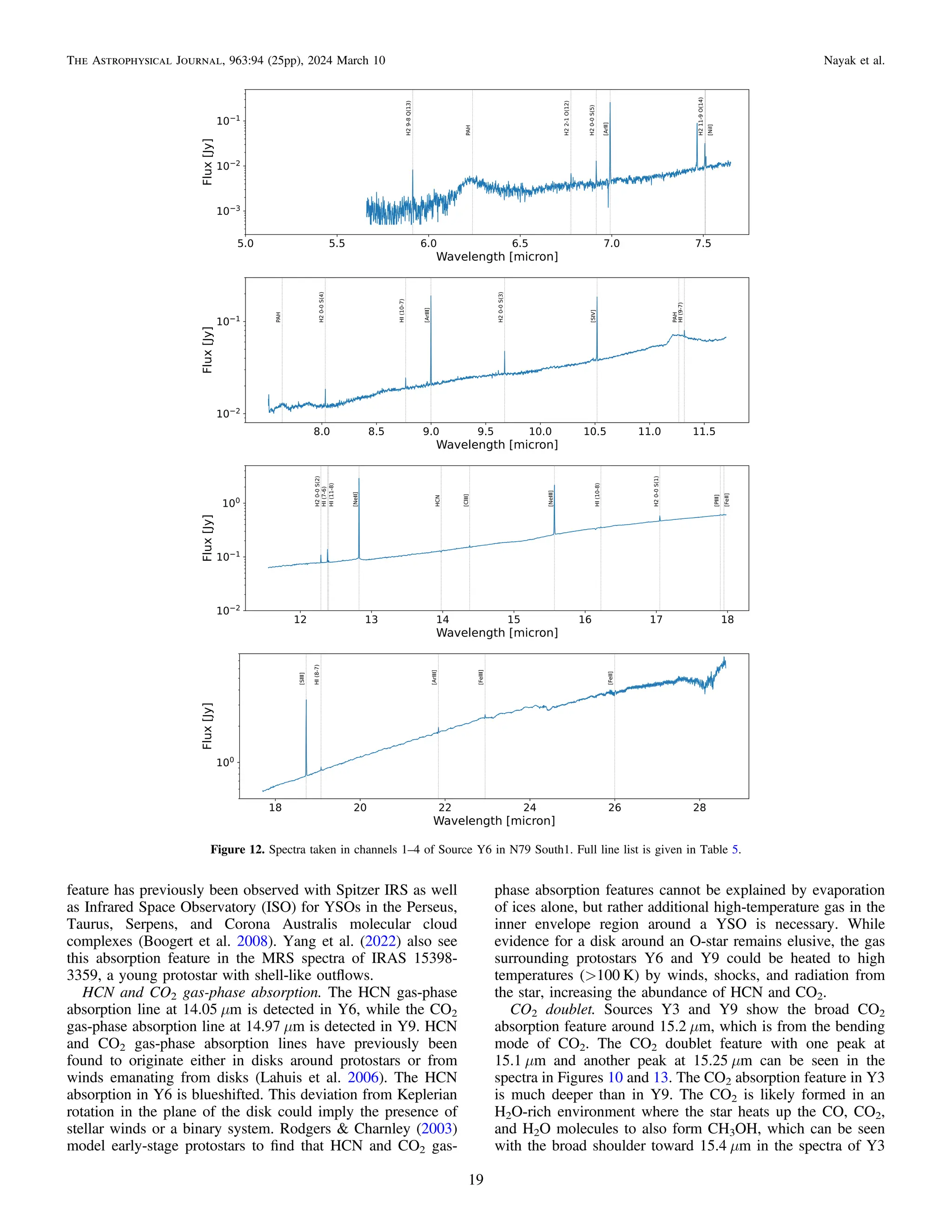
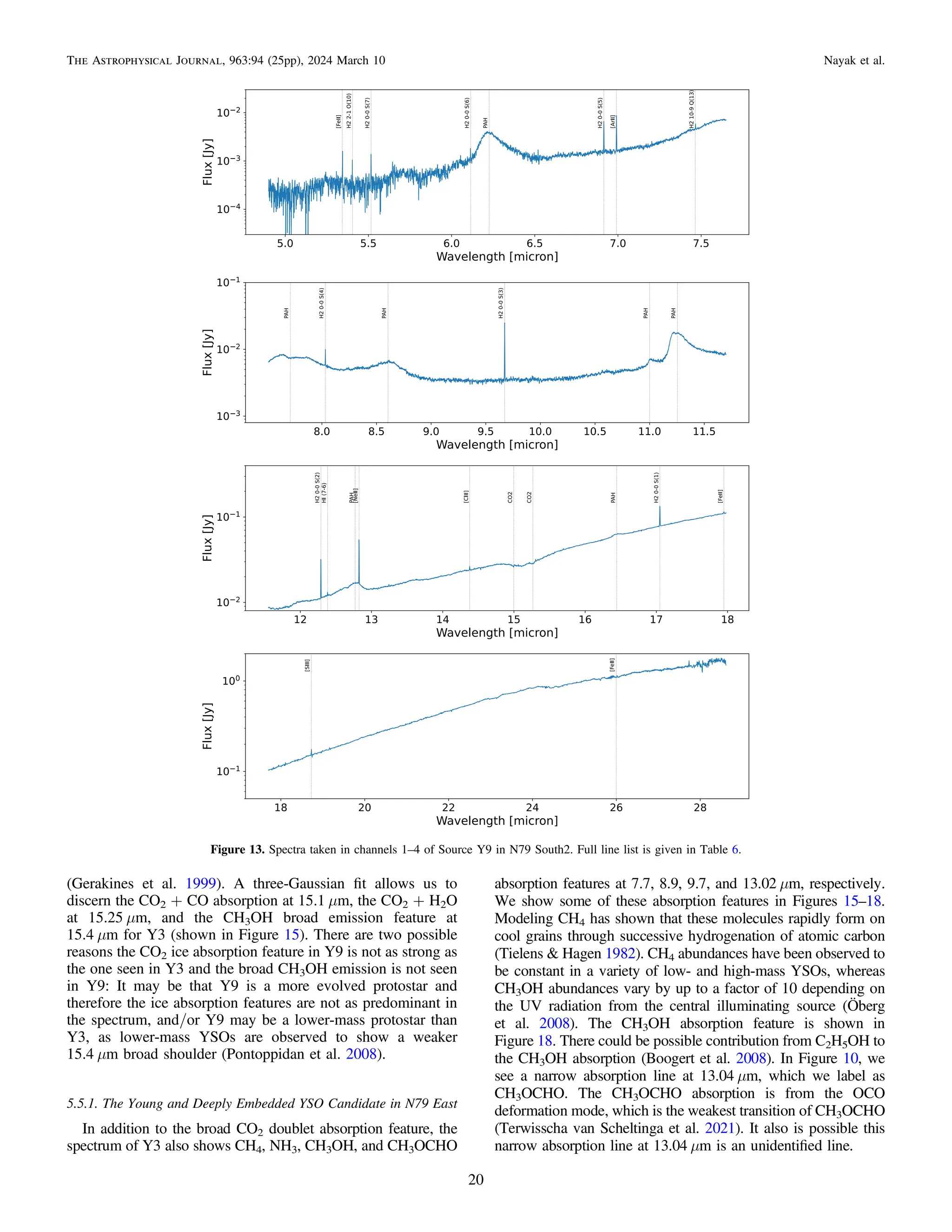
7. We detect solid- and gas-phase absorption features in the
spectra of Y1, Y3, Y4, Y6, and Y9. YSO Y2 has no absorption
features. One possible explanation for the HCN and CO2 gas-
phase absorption features in Y6 and Y9 is that high-velocity
winds are heating the surrounding gas to 100 K or higher,
leading to an increase in their abundances. Y3 and Y9 also
have the CO2 doublet feature, with Y3 having the most
prominent absorption lines. YSO Y3 has five prominent
absorption lines, likely because this source is less than
10,000 yr old.
Acknowledgments
This research relied on the following resources: NASA’s
Astrophysics Data System and the SIMBAD and VizieR
databases, operated at the Centre de Données Astronomiques
de Strasbourg, France. This research also made use of Astropy
(http://www.astropy.org), a community-developed core Python
package for Astronomy (Astropy Collaboration et al. 2013,
2018, 2022). This work is based on observations made with the
NASA/ESA/CSA James Webb Space Telescope. The JWST
data presented in this paper were obtained from the Mikulski
Archive for Space Telescopes (MAST) at the Space Telescope
Science Institute. The specific observations analyzed can be
accessed via doi:10.17909/3rz0-0e55. These observations are
associated with program #1235.
O.N. was supported by the Director’s Discretionary Fund at
the Space Telescope Science Institute and the NASA
Postdoctoral Program at NASA Goddard Space Flight Center,
administered by Oak Ridge Associated Universities under
contract with NASA. M.M. and N.H. acknowledge that a
portion of their research was carried out at the Jet Propulsion
Laboratory, California Institute of Technology, under a
contract with the National Aeronautics and Space Administra-
tion (80NM0018D0004). A.S.H. is supported in part by an
STScI Postdoctoral Fellowship. L.L. acknowledges support
from the NSF through grant 2054178. O.C.J. acknowledges
support from an STFC Webb fellowship. C.N. acknowledges
the support of an STFC studentship. P.J.K. acknowledges
support from the Science Foundation Ireland/Irish Research
Council Pathway program under grant No. 21/PATH-S/9360.
Appendix
We describe the emission and absorption lines that we could
not identify in more detail in Table A1.
23
The Astrophysical Journal, 963:94 (25pp), 2024 March 10 Nayak et al.](https://image.slidesharecdn.com/nayak2024apj96394-250127005706-08738261/75/JWST-Mid-infrared-Spectroscopy-Resolves-Gas-Dust-and-Ice-in-Young-Stellar-Objects-in-the-Large-Magellanic-Cloud-23-2048.jpg)

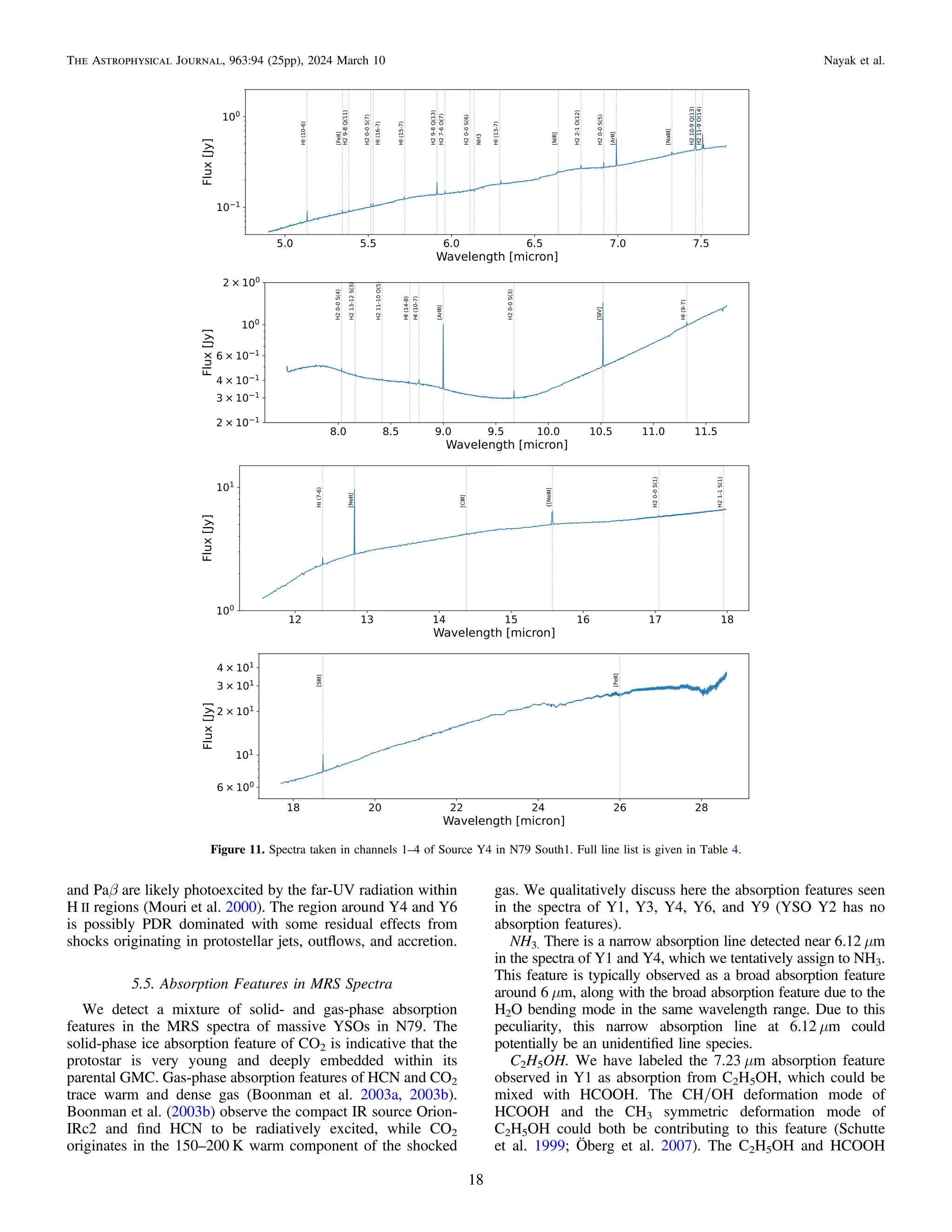
![[C II] observations made with the Stratospheric Observatory for
Infrared Astronomy (SOFIA) suggest the N79 South GMC is a
photon-dominated region (PDR) with possible shocks exciting
the CO (16–15) and CO (11–10) emission lines (Nayak et al.
2021). In this work, we are able to resolve the cluster of five
protostars in H72.97-69.39 with Mid-Infrared Instrument
(MIRI)/Medium Resolution Spectroscopy (MRS) observa-
tions. Additionally, we observe two other massive clusters,
one in the South GMC and another in the East GMC. The
source we observe in N79 West is a single protostar. Our
observations reveal how multiple massive YSOs forming
within a cluster affect local gas conditions.
YSOs are enshrouded by dust and gas, which serves as a
reservoir during the main initial accretion phase (McKee &
Ostriker 2007). UV radiation from the central illuminating
source is absorbed and then reradiated at mid- and far-infrared
(IR) wavelengths (Churchwell 2002). The observed IR spectral
emission and absorption lines can reveal the age, mass, and
accretion properties of the central protostar as well as the
temperature and ionized conditions of the surrounding ISM
(Boonman et al. 2003b; Oliveira et al. 2009; Seale et al. 2009;
Rigliaco et al. 2015). Our observations in this work reveal that
objects identified as protostars with previous Spitzer Infrared
Spectrometer (IRS) are actually small clusters, which we can
now resolve with MRS.
We observe a variety of early- and late-stage YSOs in the
South, East, and West GMCs. The spectral features of the six
YSOs we discuss in detail include H2 emission, polyaromatic
hydrocarbon (PAH) emission, silicate absorption, and solid-
and gas-phase ice absorption. Additionally, we observe for the
first time rest-frame mid-IR hydrogen recombination lines
associated with extragalactic star formation with high-resolu-
tion MRS spectra.
The mid-IR H2 originates either from UV radiation from
massive stars or collisional excitation from shocks heating the
molecular gas (Tielens et al. 1993; Hollenbach 1997). The
same UV photons collide with PAH molecules, which in turn
(1) leads to the excitation of various bending and stretching
modes and (2) breaks down large-sized PAH molecules into
smaller ones (Tielens et al. 1993; Peeters et al. 2017). Electrons
ejected from PAH molecules can further heat up the local gas,
(i.e., via the photoelectric effect). Excess H2 emission relative
to PAH emission lines has been observed in active galactic
nuclei (Ogle et al. 2010) and ultraluminous galaxies Higdon
et al. (2006), and it is thought to originate from shocks.
Hydrogen recombination lines are commonly used as a proxy
for accretion rates in YSOs, because of the empirical relation-
ship between H I luminosity and accretion luminosity across a
variety of environments (Calvet et al. 2004; Herczeg &
Hillenbrand 2008). The presence of silicate and ice absorption
lines with little to no H2 and fine-structure emission lines is
indicative of the very young protostars embedded within their
natal gas cloud, where the UV photons from the central star
have yet to ionize the surrounding gas (Oliveira et al. 2013).
The various emission and absorption lines identified in a
spectrum indicate the age of the central protostar as well as
PAH grain size distribution and ionization, plus the origin of
shocks. In this work, we further discuss and interpret the
emission and absorption lines seen in YSOs in N79.
We refer to the four Spitzer-identified sources as W1, E1, S1,
and S2, based on their respective locations in the West, East,
and South GMCs. We call the individual protostars resolved
with MIRI within the Spitzer-identified clusters “YSOs,” with
Y1 located in W1, Y2 and Y3 located in E1, Y4–Y8 in S1, and
Y9–Y11 in S2. In this study, we present MRS observations of
11 YSOs in the N79 region of the LMC, six of which have full
or nearly full mid-IR spectral coverage from 4.9–27.9 μm. The
science goal of this program is to map out the excitation and
physical conditions of the gas in order to better understand
YSO formation at different evolutionary stages. In order to
achieve our science goal, we extract the emission and
absorption lines of the six YSOs with full or nearly full mid-
IR spectral coverage and infer the conditions of the accreting
protostar and the surrounding ISM. Follow-up papers will
model the emission and absorption lines in greater detail.
In Section 2, we describe the source selection strategy and
the observation details. The data processing and resulting
catalog of spectral features are discussed in Section 3. The
Spitzer IRS spectra and photometry of the four MRS
observations are discussed in Section 4, while Section 5 goes
into the details of the YSOs resolved with the JWST MRS
observations. We summarize our results in Section 6.
2. Observation and Source Selection Strategy
We present observations of the N79 region taken with MIRI
(Rieke et al. 2015; Wright et al. 2023) on board JWST as part
of GTO program 1235 (PI: Meixner). The observations were
taken using MRS, an integral field unit (IFU) equipped with
four channels (1, 2, 3, and 4). The channels cover a wavelength
range of 4.90–7.65 μm, 7.51–11.70 μm, 11.55–17.98 μm, and
17.70–27.90 μm, respectively. Channels 1 and 2 have a higher
spectral resolution (R = 2700–3700) in comparison to Chan-
nels 3 and 4 (R = 1600–2800). In contrast, Channels 1 and 2
have a smaller field of view (FOV; 10–20 arcsec2
) in
comparison to Channels 3 and 4 (32–51 arcsec2
; Gardner
et al. 2023). Each Channel is further subdivided into three
subbands (i.e., A, B, and C), which consist of a “SHORT,”
“MEDIUM,” and “LONG” portion of the wavelength range,
respectively. As each MRS Channel possesses the same three
subbands (i.e., 1A, 1B, 1C, 2A, 2B, 2C, etc.), a full spectrum
can therefore be observed with three exposures, typically
accomplished within a single observation setup.
We use the MRS instrument to take observations of SSC
candidate H72.97-69.39, which is a superluminous source with
L = 2.2 × 10⁶
Le, and three other Spitzer-identified massive
YSO candidates in the N79 region (Ochsendorf et al. 2017).
Based on their locations within the N79 South, East, and West
GMCs, we label the Spitzer-identified YSO candidates as S1,
S2, E1, and W1. W1 was observed on 2022 November 14, and
E1 was observed on 2022 November 29. Observations of
H72.97-69.39 (labeled S1) and S2 were taken on 2022
November 30. Figure 1 shows the Spitzer 8 μm observations
of the N79 region and the location of the four MRS
observations.
The SSC candidate H72.97-69.39 was observed with MRS
using the FASTR1 readout mode for a standard four-point
dither pattern, and an assumption that the source is extended.
We use five groups/integration and five integrations/exposure
with a total exposure time for the three subbands SHORT,
MEDIUM, and LONG of 321 s. The three other Spitzer-
identified sources S2, E1, and W1 are observed with the same
readout mode and dither pattern. These YSO candidates are
less luminous than H72.97-69.39, and therefore we use 13
2
The Astrophysical Journal, 963:94 (25pp), 2024 March 10 Nayak et al.](https://crownmelresort.com/image.slidesharecdn.com/nayak2024apj96394-250127005706-08738261/75/JWST-Mid-infrared-Spectroscopy-Resolves-Gas-Dust-and-Ice-in-Young-Stellar-Objects-in-the-Large-Magellanic-Cloud-2-2048.jpg)
![groups/integration and two integrations/exposure for a total
exposure time of 299 s per target.
MRS observations of S1, S2, and E1 show that what was
observed to be a single source with Spitzer is actually a cluster of
two to five less-massive YSOs. Source W1, however, is an
isolated YSO. There are a total of 11 YSOs within the four MRS
observations. We chose a variety of early- and late-stage YSO
candidates based on their spectral features seen with Spitzer IRS
observations.
3. Data Processing
3.1. MIRI MRS Pipeline Processing
The JWST MRS observations were processed using pipeline
version 1.11.0 with jwst_1094.pmap context (Bushouse et al.
2023). This pipeline version uses time-dependent photometric
corrections, has the ability to set the outlier detection kernel
size and threshold, and implements residual fringe correction
during the spectral extraction process. We use the standard
detector corrections calwebb_detector1 and calwebb_spec2
during Stage 1 and Stage 2 of the data reduction process
(Labiano et al. 2016), with the residual_fringe step switched
on. The residual fringe correction step applies additional fringe
correction arising from the difference between fringe pattern on
the detector from an extended source and the standard pipeline
fringe flat. Stage 3 of the pipeline (calwebb_spec3) includes the
outlier_detection and spectrum level residual fringe correction
(ifu_rfcorr) routines. The outlier detection step compares a
median taken from stacked images to the original images, to
determine if there are bad pixels or cosmic rays. We set the size
of the kernel used to normalize the pixel difference in the
outlier detection step to be 11 pixels. Even after the fringe and
residual fringe corrections applied with the standard pipeline
steps, there can still be fringe residuals in extracted spectra; in
particular, there is often high-frequency fringing present in
channels 3 and 4, thought to arise from the dichroics, which are
difficult to remove at the detector level. We used the
(ifu_rfcorr) step on extracted spectra to reduce the contrast of
the fringes that remain.
The spectrum of each of the 11 YSOs detected in the four MRS
pointings is extracted with an aperture defined as 1.22 λ/D,
where λ is the wavelength of the IFU cube and D is the beam size.
The background is similarly calculated by extracting a spectrum
within the spectral cube, but away from the bright point sources.
After background subtraction, the 12 spectral cube segments are
scaled in a consecutive manner using a median flux value between
two consecutive subbands such that channel 1B is scaled to 1A,
and then channel 1C is scaled to 1B, and so forth. The resulting
spectral segments are stitched together using the combine_1d step
of the JWST pipeline. Figure 2 shows the MRS spectra of the 11
sources in this work as well as Spitzer IRS spectra of S1, S2, E1,
and W1.
We fit a continuum to the spectra extracted in each subband
using the spline function in the astropy package. After subtracting
the continuum, the emission and absorption lines are detected with
find_lines_threshold function from specutils. The lines are fit with
a Gaussian profile, and their parameters (measured wavelength,
uncertainty in wavelength, FWHM, flux, and uncertainty in flux)
are listed in Tables 1–6. Table 7 summarizes the emission and
absorption lines seen in the spectra of Y1, Y2, Y3, Y4, Y6,
and Y9. Taking into account the radial velocity of N79
(235 km s−1
; Nayak et al. 2019), the narrow emission and
absorption features are matched to the closest known H2, HI, fine-
structure, or ice lines within 0.01 μm. If there are multiple
matches, then the closest laboratory emission or absorption line is
selected to be the observed line. The broad PAH emission line and
ice absorption lines are determined by matching the observed
features to the known laboratory lines, with the requirement that
λobserved − λlaboratory < 0.05. We list the emission and absorption
lines we are unable to identify in Appendix Table A1; these are
due to warm pixels, fringe flat correction issues, undersampling,
and stitching effects in overlap channels.
3.2. Catalog of Spectral Features
Figures 3–6 show cube slices at 5.51, 6.20, 11.20, 12.81,
17.04, and 18.71 μm, which trace H2 5.51 μm, PAH features,
[Ne II], H2 17.04 μm, and [S III] emission lines, respectively.
The YSOs in each region are labeled Y1 through Y11. The
spectra for YSOs Y1 located in the N79 West GMC, Y2 in the
East GMC, and Y4 in the South GMC observation cover the
full MRS wavelength range from 4.9–27.9 μm. Y3 located in
N79 East is very faint in Channel 1. The extracted spectrum for
this source is noisy, with little to no signal in wavelengths
shorter than 7.5 μm. Sources Y6 in S1 and Y9 in S2 are noisy
in Channel 1A, and therefore the spectra shown for these two
sources in Figure 2 are for 1B and longer wavelengths. YSOs
Y5, Y7, and Y8 are on the edge of the MRS FOV in Channels
1 and 2 (Figure 5); therefore, they do not have the full spectral
coverage. Additionally, the emission lines seen in YSOs Y5,
Y7, and Y8 are the same as the emission lines seen in Y6,
which can be seen in Figure 2. The similarity in emission line
species and line strength between the three YSOs in region S1
to Y6 implies the three protostars are not the dominating source
in the MRS FOV. Y10 and Y11 are also on the edge of
Channel 1, which is shown in Figure 6, and therefore they do
not have full spectral coverage of MRS.
In this work, we discuss sources Y1, Y2, Y3, Y4, Y6, and
Y9 in further detail. Sources Y5, Y7, Y8, Y10, and Y11 are
Figure 1. Spitzer IRAC 8.0 μm image of the N79 region. We highlight the
location of the MRS footprint with the four red circles. The red circles have a
diameter of 70″, much larger than the MRS footprint. We selected these four
sources because previous Spitzer IRS spectral observations indicated these are
indeed YSOs, in addition to SED models indicating that these YSOs are very
massive (over 8 Me).
3
The Astrophysical Journal, 963:94 (25pp), 2024 March 10 Nayak et al.](https://crownmelresort.com/image.slidesharecdn.com/nayak2024apj96394-250127005706-08738261/75/JWST-Mid-infrared-Spectroscopy-Resolves-Gas-Dust-and-Ice-in-Young-Stellar-Objects-in-the-Large-Magellanic-Cloud-3-2048.jpg)

![stages of formation, YSOs are enshrouded by dust and gas.
Their radiation is absorbed by the dust and gas, and
subsequently reprocessed to output emission at far-IR
wavelengths. Herschel Photoconductor Array Camera and
Spectrometer (PACS) and Spectral and Photometric Imaging
Receiver (SPIRE) data cover the far-IR wavelength range of
70–500 μm, allowing for the identification of the youngest
and most-embedded YSO candidates. Seale et al. (2014)
found 2493 YSO candidates using Spitzer and Herschel
photometry, 73% of which were not identified with previous
studies that only used Spitzer.
The angular resolution of Spitzer and Herschel ranges from
1 7 in the IRAC 3.6 μm band to 40 5 in the SPIRE 500 μm
band. Channel 1 MIRI/MRS observations have an FOV that is
3 2 × 3 7. Our MRS observations reveal that what appeared
to be a single YSO in Spitzer and Herschel observations is
actually a small cluster of YSOs in S1, S2, and E1. MRS
observations of W1 reveal a single YSO.
We use the Spitzer and Herschel photometry from Gruendl
& Chu (2009) and Seale et al. (2014) to fit spectral energy
distribution (SED) models to get estimates of the total masses
and luminosities of the clusters in E1, S1, and S2, and of the
isolated YSO in W1. The “spbhmi” Robitaille (2017) SED
model grid used in this work includes 10,000 model YSOs with
a wide range of parameters: stellar radius (0.1–100 Re), stellar
temperature (2000–30,000 K), disk mask (10−8
–10−1
Me),
outer disk radius (50–5000 au), envelope density
(10−24
–10−16
g cm−3
), envelope power law (−2 to −1), cavity
density (10−23
–10−20
g cm−3
), and cavity opening angle (0°–
60°). Figure 7 shows the Robitaille (2017) best-fit SED models
Table 1
Source Y1 Emission and Absorption Lines
Name Absorption or Lab Wave Meas Wave Meas Wave Err FWHM Flux Flux Err
Emission (μm) (μm) (μm) (μm) (erg s−1
cm−2
) (erg s−1
cm−2
)
H2 10-9 Q(2) E 4.987 4.99115 0.00125 0.00093 8.815E-17 1.122E-16
H I (10-6) E 5.129 5.13902 0.00138 0.00138 5.369E-17 1.070E-16
H2 5-5 S(13) E 5.291 5.29989 0.00109 0.00129 1.005E-16 1.079E-16
[Fe II] a4F9/2-a6D9/2 E 5.340 5.34462 0.00013 0.00136 3.631E-16 1.145E-16
H2 7-6 O(6) E 5.415 5.42082 0.00012 0.00657 3.573E-16 1.121E-16
H2 0-0 S(7) E 5.511 5.51660 0.00100 0.00176 2.348E-16 1.030E-16
H2 9-8 Q(13) E 5.909 5.91066 0.00174 0.00167 1.135E-16 1.231E-16
NH3 A 6.150 6.12035 0.00033 0.00437 4.060E-16 1.043E-16
PAH E 6.200 6.22776 0.00077 0.10208 2.972E-14 7.087E-16
[Ni II] 2D3/2-2D5/2 E 6.636 6.64202 0.00122 0.00232 1.319E-16 1.029E-16
H2 0-0 S(5) E 6.910 6.91495 0.00025 0.00208 7.061E-16 1.035E-16
[Ar II] 2P1/2-2P3/2 E 6.985 6.99076 0.00044 0.00199 3.713E-15 1.367E-16
C2H5OH A 7.240 7.22451 0.00035 0.00661 4.094E-16 8.805E-17
H2 8-8 S(12) E 7.323 7.33174 0.00346 0.00124 9.381E-17 9.875E-17
H2 10-9 Q(13) E 7.452 7.46514 0.00046 0.00230 7.573E-16 1.078E-16
H2 11-9 O(14) E 7.507 7.50931 0.00131 0.00197 1.026E-16 1.039E-16
PAH E 7.700 7.64696 0.00649 0.12591 5.838E-14 9.781E-16
PAH E 7.700 7.84175 0.00857 0.11913 5.252E-14 8.866E-16
H2 0-0 S(4) E 8.025 8.03197 0.00002 0.00208 4.252E-16 2.013E-16
PAH E 8.600 8.64508 0.00313 0.60429 1.569E-13 2.585E-15
[Ar III] 3P1-3P2 E 8.991 8.99895 0.00070 0.00294 4.512E-16 1.470E-16
H2 3-3 S(4) E 9.431 9.43722 0.00087 0.00161 7.016E-17 1.111E-16
H2 0-0 S(3) E 9.665 9.67298 0.00003 0.00257 9.457E-16 1.093E-16
[S IV] 2P3/2-2P1/2 E 10.511 10.51908 0.00013 0.00331 3.934E-16 1.959E-16
PAH E 11.000 11.00937 0.01351 0.04045 2.485E-15 2.633E-15
PAH E 11.200 11.25099 0.00086 0.12722 5.593E-14 1.194E-15
(9-7) E 11.310 11.31906 0.00191 0.00306 3.124E-16 8.245E-17
H2 0-0 S(2) E 12.279 12.28917 0.00042 0.00358 6.591E-16 2.709E-16
H I (7-6) E 12.370 12.38198 0.00073 0.00458 1.289E-15 3.953E-16
PAH E 12.700 12.759794 0.00363 0.24805 3.061E-14 1.423E-15
[Ne II] 2P1/2-2P3/2 E 12.814 12.82427 0.00052 0.00430 3.216E-14 6.875E-16
H2 5-4 O(15) E 13.828 13.84260 0.00115 0.00306 7.150E-17 2.483E-16
[Cl II] 3P1-3P2 E 14.368 14.37880 0.00005 0.00424 3.582E-16 2.608E-16
[Ne III] 3P1-3P2 E 15.555 15.56790 0.00085 0.00640 1.750E-15 2.698E-16
PAH E 16.400 16.43141 0.00355 0.08704 6.57E-15 8.51E-16
H2 0-0 S(1) E 17.035 17.04974 0.00099 0.00576 2.091E-15 3.982E-16
[P III] 2P3/2-2P1/2 E 17.885 17.89816 0.00058 0.00641 3.619E-16 4.472E-16
[Fe II] a4F7/2-a4F9/2 E 17.936 17.94813 0.00201 0.00667 6.665E-16 3.848E-16
[S III] 3P2-3P1 E 18.713 18.72723 0.00178 0.00938 3.702E-14 2.742E-15
[Fe III] 5D3-5D4 E 22.925 22.94277 0.00023 0.00936 2.592E-15 2.031E-15
[Fe II] a6D7/2-a6D9/2 E 25.998 26.01579 0.00101 0.01069 8.920E-15 2.534E-15
Notes. Column (1): Name of line. Column (2): Emission or absorption line. “E” stands for emission, and “A” stands for absorption. Column (3): Laboratory
wavelength. Column (4): Measured wavelength. Column (5): Error in measured wavelength. Column (6): FWHM of line. Column (7): Measured flux. Column (8):
Error in flux.
5
The Astrophysical Journal, 963:94 (25pp), 2024 March 10 Nayak et al.](https://crownmelresort.com/image.slidesharecdn.com/nayak2024apj96394-250127005706-08738261/75/JWST-Mid-infrared-Spectroscopy-Resolves-Gas-Dust-and-Ice-in-Young-Stellar-Objects-in-the-Large-Magellanic-Cloud-5-2048.jpg)
![fit to the observed mid-IR and far-IR data. The Spitzer IRAC
observations are in black circles, and the Spitzer MIPS and
Herschel observations are in black triangles, fitted as upper
limits. The beam sizees of the Spitzer MIPS, Herschel PACS,
and Herschel SPIRE observations range from 6″–35″ (Meixner
et al. 2006, 2013). Mid- and far-IR emission from the central
protostar and the surrounding dust will be unresolved by the
MIPS, PACS, and SPIRE, due to the beam size being much
larger than the 1″–2″ beam size of IRAC (Meixner et al. 2006).
Therefore, the mid- and far-IR photometry are fit as upper
limits when we use the SED models. The best-fit models for
sources E1, S1, and S2 show a rise in flux toward mid-IR
wavelengths, which is typical for YSOs. The best-fit model for
source W1 is a more evolved YSO, as inferred from the SED:
There is some IR emission seen with the bump around 100 μm;
however, the optical light from the star is also seen in the SED
with the bump around 10 μm.
The masses of clusters E1, S1, S2, and the isolated YSO Y1
in W1 determined by fitting the SEDs with Robitaille (2017)
models are 18.3 ± 2.7, 25.4 ± 3.2, 15.7 ± 4.5, and 13.6 ±
1.6 Me, respectively. The luminosities of E1, S1, S2, and
W1 are 4.1 ± 1.9 × 10⁴
, 1.2 ± 0.5 × 10⁵
, 3.1 ± 1.2 × 10⁴
, and
Table 2
Source Y2 Emission and Absorption Lines
Name Absorption or Lab Wave Meas Wave Meas Wave Err FWHM Flux Flux Err
Emission (μm) (μm) (μm) (μm) (erg s−1
cm−2
) (erg s−1
cm−2
)
H I (10-6) E 5.129 5.13263 0.00057 0.00182 4.748E-16 6.219E-17
[Fe II] a4F9/2-a6D9/2 E 5.340 5.34461 0.00006 0.00137 5.551E-16 8.300E-17
H2 9-8 Q(11) E 5.373 5.38499 0.00059 0.00167 9.680E-17 4.856E-17
H2 0-0 S(7) E 5.511 5.51671 0.00111 0.00173 2.866E-16 4.758E-17
H2 8-7 Q(15) E 5.540 5.53164 0.00244 0.00185 1.542E-16 4.724E-17
H I (15-7) E 5.711 5.71989 5.71989 0.00151 1.464E-16 4.922E-17
H2 9-8 Q(13) E 5.909 5.91320 0.00000 0.00210 8.560E-16 7.946E-17
H2 7-6 O(7) E 5.956 5.96141 0.00021 0.00198 1.063E-16 5.994E-17
H2 0-0 S(6) E 6.109 6.11391 0.00009 0.00205 2.376E-16 6.366E-17
PAH E 6.200 6.22780 0.00037 0.10271 8.871E-14 9.380E-16
H I (13-7) E 6.292 6.29757 0.00037 0.00175 2.356E-16 8.179E-17
[Ni II] 2D3/2-2D5/2 E 6.636 6.64164 0.00004 0.00214 2.863E-16 4.431E-17
H2 2-1 O(12) E 6.776 6.77758 0.00002 0.00200 3.273E-16 4.541E-17
H2 0-0 S(5) E 6.910 6.91527 0.00006 0.00218 1.281E-15 5.278E-17
[Ar II] 2P1/2-2P3/2 E 6.985 6.99117 0.00003 0.00200 4.019E-14 7.912E-16
H2 1-1 S(5) E 7.280 7.27795 0.00035 0.00191 1.116E-16 4.386E-17
[Ni III] 3F4-3F34 E 7.349 7.35930 0.00089 0.00209 3.675E-16 5.095E-17
H2 10-9 Q(13) E 7.452 7.46605 0.00035 0.00200 7.606E-15 1.727E-16
H2 11-9 O(14) E 7.507 7.50953 0.00073 0.00207 1.951E-15 8.293E-17
[Ni I] a3F3-a3F4 E 7.507 7.51097 0.00343 0.00108 5.058E-16 6.366E-17
PAH E 7.700 7.61215 0.01997 0.28076 3.900E-13 2.741E-15
PAH E 7.700 7.84645 0.01984 0.21193 2.769E-13 1.968E-15
H I (16-8) E 7.780 7.79157 0.00532 0.00269 6.172E-17 2.000E-16
H2 0-0 S(4) E 8.025 8.03199 0.00004 0.00215 8.687E-16 1.519E-16
H2 13-12 S(3) E 8.148 8.16010 0.00185 0.00313 1.188E-16 1.400E-16
PAH E 8.600 8.61029 0.00532 0.23580 5.719E-14 4.092E-15
H I (10-7) E 8.760 8.76749 0.00066 0.00326 4.637E-16 6.774E-17
[Ar III] 3P1-3P2 E 8.991 8.99889 0.00066 0.00295 3.377E-15 1.458E-16
H I (13-8) E 9.329 9.40022 0.00027 0.00230 7.797E-17 4.239E-17
H2 0-0 S(3) E 9.665 9.67309 0.00014 0.00239 1.748E-15 5.295E-17
[S IV] 2P3/2-2P1/2 E 10.511 10.51739 0.00286 0.00357 7.523E-17 7.825E-17
PAH E 11.000 11.01255 0.01518 0.04319 4.270E-15 4.765E-15
PAH E 11.200 11.25264 0.00088 0.13145 9.979E-14 2.124E-15
H I (9-7) E 11.310 11.31796 0.00049 0.00317 1.089E-15 8.138E-17
H2 0-0 S(2) E 12.279 12.28923 0.00048 0.00393 2.596E-15 3.061E-16
H I (7-6) E 12.370 12.38270 0.00105 0.00545 6.634E-15 8.583E-16
H I (11-8) E 12.387 12.39815 0.00060 0.00597 8.307E-16 2.907E-16
PAH E 12.700 12.75113 0.00605 0.24369 5.321E-14 4.201E-15
[Ne II] 2P1/2-2P3/2 E 12.814 12.82466 0.00091 0.00493 1.617E-13 3.307E-15
[Cl II] 3P1-3P2 E 14.368 14.37897 0.00022 0.00382 8.129E-16 4.088E-16
[Ne III] 3P1-3P2 E 15.555 15.56927 0.00052 0.00569 5.001E-16 6.220E-16
PAH E 16.400 16.44669 0.00285 0.08292 1.151E-14 1.258E-15
H2 0-0 S(1) E 17.035 17.05001 0.00124 0.00581 4.152E-15 8.730E-16
[S III] 3P2-3P1 E 18.713 18.72859 0.00041 0.00803 7.605E-14 5.615E-15
[Fe III] 5D3-5D4 E 22.925 22.94417 0.00117 0.00992 7.756E-15 6.346E-15
[Fe II] a6D7/2-a6D9/2 E 25.998 26.01564 0.00169 0.01007 1.659E-14 8.436E-15
Notes. Column (1): Name of line. Column (2): Emission or absorption line. “E” stands for emission, and “A” stands for absorption. Column (3): Laboratory
wavelength. Column (4): Measured wavelength. Column (5): Error in measured wavelength. Column (6): FWHM of line. Column (7): Measured flux. Column (8):
Error in flux.
6
The Astrophysical Journal, 963:94 (25pp), 2024 March 10 Nayak et al.](https://crownmelresort.com/image.slidesharecdn.com/nayak2024apj96394-250127005706-08738261/75/JWST-Mid-infrared-Spectroscopy-Resolves-Gas-Dust-and-Ice-in-Young-Stellar-Objects-in-the-Large-Magellanic-Cloud-6-2048.jpg)
![Table 3
Source Y3 Emission and Absorption Lines
Name Absorption or Lab Wave Meas Wave Meas Wave Err FWHM Flux Flux Err
Emission (μm) (μm) (μm) (μm) (erg s−1
cm−2
) (erg s−1
cm−2
)
CH4 A 7.700 7.68265 0.00209 0.05443 3.312E-15 4.038E-16
H2 0-0 S(4) E 8.025 8.03164 0.00031 0.00231 3.917E-16 1.183E-16
NH3 A 9.000 8.93675 0.00212 0.30607 3.524E-14 7.778E-16
H2 0-0 S(3) E 9.665 9.67342 0.00047 0.00291 7.907E-16 2.746E-17
CH3OH A 9.700 9.73806 0.00289 0.35165 5.140E-14 1.340E-15
H2 9-8 O(10) E 10.974 10.97567 0.00868 0.00113 4.793E-18 4.697E-17
PAH E 11.200 11.27072 0.00190 0.14982 1.038E-14 4.178E-16
H I (23-10) E 11.243 11.25589 0.00405 0.00139 3.282E-17 4.861E-17
H2 0-0 S(2) E 12.279 12.28930 0.00055 0.00425 1.393E-15 7.711E-17
[Ne II] 2P1/2-2P3/2 E 12.814 12.82459 0.00084 0.00506 1.254E-15 7.040E-17
CH3OCHO A 13.020 13.04829 0.00046 0.00311 8.629E-17 6.287E-17
CO2 A 15.200 15.19246 0.00152 0.46127 3.636E-13 3.096E-14
[Ne III] 3P1-3P2 E 15.555 15.56852 0.00023 0.00568 2.579E-16 7.367E-17
H2 0-0 S(1) E 17.035 17.04969 0.00094 0.00576 2.577E-15 9.930E-17
[S III] 3P2-3P1 E 18.713 18.72850 0.00056 0.00841 2.106E-15 3.365E-16
Notes. Column (1): Name of line. Column (2): Emission or absorption line. “E” stands for emission, and “A” stands for absorption. Column (3): Laboratory
wavelength. Column (4): Measured wavelength. Column (5): Error in measured wavelength. Column (6): FWHM of line. Column (7): Measured flux. Column (8):
Error in flux.
Table 4
Source Y4 Emission and Absorption Lines
Name Absorption or Lab Wave Meas Wave Meas Wave Err FWHM Flux Flux Err
Emission (μm) (μm) (μm) (μm) (erg s−1
cm−2
) (erg s−1
cm−2
)
[Fe II] a4F9/2-a6D9/2 E 5.340 5.34442 0.00010 0.00135 1.937E-15 3.752E-16
H2 9-8 Q(11) E 5.373 5.38409 0.00031 0.00184 8.636E-16 1.003E-15
H2 0-0 S(7) E 5.511 5.51550 0.00010 0.00118 1.086E-15 1.046E-15
H I (10-6) E 5.129 5.13282 0.00038 0.00185 4.521E-15 1.013E-15
H I (16-7) E 5.525 5.53040 0.00040 0.00180 1.226E-15 1.065E-15
H I (15-7) E 5.711 5.71673 0.00034 0.00223 1.523E-15 1.406E-15
H2 9-8 Q(13) E 5.909 5.91294 0.00026 0.00220 9.763E-15 1.486E-15
H2 7-6 O(7) E 5.956 5.96132 0.00068 0.00212 1.346E-15 1.372E-15
H2 0-0 S(6) E 6.109 6.11192 0.00128 0.00161 7.511E-16 1.345E-15
NH3 A 6.150 6.13673 0.00010 0.00328 2.133E-15 1.295E-15
H I (13-7) E 6.292 6.29676 0.00044 0.00191 2.348E-15 1.498E-15
[Ni II] 2D3/2-2D5/2 E 6.636 6.64181 0.00021 0.00218 1.981E-15 1.631E-15
H2 2-1 O(12) E 6.776 6.77762 0.00002 0.00263 4.722E-15 1.730E-15
H2 0-0 S(5) E 6.910 6.91518 0.00002 0.00159 4.481E-15 1.668E-15
[Ar II] 2P1/2-2P3/2 E 6.985 6.99120 0.00000 0.00201 3.873E-14 2.128E-15
[Na III] 2P1/2-2P3/2 E 7.318 7.32457 0.00057 0.00363 5.462E-15 2.121E-15
H2 10-9 Q(13) E 7.452 7.46609 0.00031 0.00216 1.026E-13 3.196E-15
H2 11-9 O(14) E 7.507 7.50919 0.00039 0.00240 3.419E-14 2.444E-15
H2 0-0 S(4) E 8.025 8.03148 0.00047 0.00264 2.865E-15 3.494E-15
H2 13-12 S(3) E 8.148 8.16118 0.00077 0.00260 1.334E-15 3.333E-15
H2 11-10 O(5) E 8.410 8.41706 0.00031 0.00282 1.340E-15 2.673E-15
H I (14-8) E 8.665 8.68037 0.00882 0.00327 5.226E-17 2.243E-15
H I (10-7) E 8.760 8.76765 0.00050 0.00333 4.061E-15 1.696E-15
[Ar III] 3P1-3P2 E 8.991 8.99884 0.00071 0.00335 9.191E-14 2.713E-15
H2 0-0 S(3) E 9.665 9.67205 0.00090 0.00305 3.947E-15 9.178E-16
[S IV] 2P3/2-2P1/2 E 10.511 10.51943 0.00048 0.00355 1.068E-13 3.065E-15
H I (9-7) E 11.310 11.31834 0.00011 0.00377 8.782E-15 2.487E-15
H I (7-6) E 12.370 12.38235 0.00140 0.00529 7.162E-14 5.798E-15
[Ne II] 2P1/2-2P3/2 E 12.814 12.82449 0.00074 0.00490 6.398E-13 1.812E-14
[Cl II] 3P1-3P2 E 14.368 14.37854 0.00021 0.00521 1.334E-14 1.131E-14
[Ne III] 3P1-3P2 E 15.555 15.57259 0.00116 0.00815 2.250E-13 9.701E-15
H2 0-0 S(1) E 17.035 17.04803 0.00072 0.00606 6.571E-15 8.205E-15
H2 1-1 S(1) E 17.933 17.94781 0.00156 0.00731 7.735E-15 8.479E-15
[S III] 3P2-3P1 E 18.713 18.72804 0.00096 0.00988 2.627E-13 4.292E-14
[Fe II] a6D7/2-a6D9/2 E 25.998 26.01279 0.00467 0.01892 1.012E-13 7.918E-14
Notes. Column (1): Name of line. Column (2): Emission or absorption line. “E” stands for emission, and “A” stands for absorption. Column (3): Laboratory
wavelength. Column (4): Measured wavelength. Column (5): Error in measured wavelength. Column (6): FWHM of line. Column (7): Measured flux. Column (8):
Error in flux.
7
The Astrophysical Journal, 963:94 (25pp), 2024 March 10 Nayak et al.](https://crownmelresort.com/image.slidesharecdn.com/nayak2024apj96394-250127005706-08738261/75/JWST-Mid-infrared-Spectroscopy-Resolves-Gas-Dust-and-Ice-in-Young-Stellar-Objects-in-the-Large-Magellanic-Cloud-7-2048.jpg)
![1.3 ± 0.6 × 10⁴
Le, respectively. The effective temperatures
are 17,000 ± 6100, 19,000 ± 5900, 17,000 ± 7000, and
11,000 ± 5500 K, respectively. S1 is the most massive cluster,
with a luminosity 1–2 orders of magnitude higher than those of
any of the other sources E1, S2, and W1. Within a cluster, a
single massive YSO typically dominates the overall luminosity
(Looney et al. 2006). Therefore, we assume Y2 dominates in
E1, Y4 dominates in S1, and Y9 dominates in S2. Y1 is an
isolated YSO in W1. With the addition of MRS observations,
we are able to analyze each individual YSO in the Spitzer- and
Herschel-identified clusters.
5. Preliminary Results of Spectra
With the IRS on board Spitzer, Seale et al. (2009) observed
H72.97-69.39 (S1) and three other YSO candidates: S2, E1, and
W1. S1 and S2 have silicate absorption features and fine-structure
emission lines, E1 has broad PAH emission and silicate
absorption features, and W1 has PAH features but not silicate
absorption. Silicate absorption features seen at 10 and 18 μm, as
well as other ice absorption features that will be described in
Section 5.5, are indicative of a young protostar embedded within
its parental clump. As a YSO evolves, the UV photons from the
central ionizing source lead to PAH and fine-structure emission
lines observed in its spectrum. The CC and CH stretching and
bending modes of PAHs trace properties of the photoelectric
effect and the heating/cooling of the ISM (Draine et al. 2007;
Tielens 2008). The fine-structure line emission is related to the
hardness of the UV radiation and can be used to determine
conditions of the shock-heated gas (Hollenbach et al. 1989).
Spitzer IRS observations of S2 show silicate absorption features
and no PAH or fine-structure emission, making this the youngest
source in our MRS observations. The other three sources in this
work have a combination of silicate absorption, PAH emission,
and fine-structure line emission.
The MRS spectra of Y1, Y2, Y3, Y4, Y6, and Y9 all show
increasing flux toward mid-IR wavelengths, a characteristic
typical of YSOs (Figure 2). Additionally, we see broad
absorption lines, broad PAH emission lines, and narrow
emission lines. The long-wavelength MRS subband 4C has a
lower signal-to-noise (S/N) ratio, making line fitting from
wavelengths 24.4 to 28.6 μm less reliable. Even in subbands
1A through 4B, the fluxes extracted from Gaussian fitting are
dependent upon determining emission- and absorption-free
ranges for continuum fitting and subtraction. Modeling the
emission lines with CLOUDY and PAHFIT will be done in a
later paper. In this work, we discuss the details of the various
Table 5
Source Y6 Emission and Absorption Lines
Name Absorption or Lab Wave Meas Wave Meas Wave Err FWHM Flux Flux Err
Emission (μm) (μm) (μm) (μm) (erg s−1
cm−2
) (erg s−1
cm−2
)
H2 9-8 Q(13) E 5.909 5.91289 0.00031 0.00209 1.237E-15 5.581E-17
PAH E 6.200 6.23934 0.00168 0.12349 4.838E-14 2.093E-15
H2 2-1 O(12) E 6.776 6.77683 0.00077 0.00248 4.536E-16 3.956E-17
H2 0-0 S(5) E 6.910 6.91559 0.00039 0.00177 1.119E-15 4.166E-17
[Ar II] 2P1/2-2P3/2 E 6.985 6.99106 0.00014 0.00147 2.919E-14 6.152E-16
H2 11-9 O(14) E 7.506 7.50930 0.00050 0.00233 3.471E-15 1.009E-16
[Ni I] a3F3-a3F4 E 7.507 7.51107 0.00333 0.00104 1.122E-15 6.581E-17
PAH E 7.700 7.63727 0.03884 0.40222 1.327E-13 4.066E-14
H2 0-0 S(4) E 8.025 8.03162 0.00033 0.00271 8.518E-16 1.387E-16
H I (10-7) E 8.760 8.76730 0.00045 0.00278 7.269E-16 1.397E-16
[Ar III] 3P1-3P2 E 8.991 8.99845 0.00020 0.00314 2.073E-14 5.794E-16
H2 0-0 S(3) E 9.665 9.67272 0.00023 0.00250 1.877E-15 1.568E-16
[S IV] 2P3/2-2P1/2 E 10.511 10.51874 0.00021 0.00290 1.274E-14 3.472E-16
PAH E 11.200 11.26670 0.00103 0.16708 1.134E-13 2.218E-15
H I (9-7) E 11.310 11.31777 0.00062 0.00322 1.940E-15 1.868E-16
H2 0-0 S(2) E 12.279 12.28880 0.00005 0.00400 2.890E-15 4.229E-16
H I (7-6) E 12.370 12.38179 0.00054 0.00468 1.013E-14 7.068E-16
H I (11-8) E 12.387 12.39659 0.00034 0.00643 1.941E-15 4.093E-16
[Ne II] 2P1/2-2P3/2 E 12.814 12.82418 0.00043 0.00411 2.285E-13 4.481E-15
HCN A 14.050 13.97779 0.00044 0.00806 1.757E-15 3.056E-16
[Cl II] 3P1-3P2 E 14.368 14.37792 0.00083 0.00459 1.223E-15 4.779E-16
[Ne III] 3P1-3P2 E 15.555 15.56774 0.00101 0.00652 1.422E-13 1.609E-15
H I (10-8) E 16.209 16.22067 0.00058 0.00703 1.552E-15 6.704E-16
H2 0-0 S(1) E 17.035 17.04911 0.00036 0.00524 5.884E-15 7.255E-16
[P III] 2P3/2-2P1/2, E 17.885 17.89809 0.00066 0.00781 1.078E-15 7.461E-16
[Fe II] a4F7/2-a4F9/2 E 17.936 17.94888 0.00125 0.00725 2.028E-15 1.110E-15
[S III] 3P2-3P1 E 18.713 18.72739 0.00161 0.00939 2.311E-13 8.686E-15
H I (8-7) E 19.062 19.07710 0.00010 0.00786 3.549E-15 5.163E-15
[Ar III] 3P0-3P1 E 21.830 21.84428 0.00072 0.00761 7.731E-15 5.142E-15
[Fe III] 5D3-5D4 E 22.925 22.94357 0.00056 0.00943 5.923E-15 5.517E-15
[Fe II] a6D7/2-a6D9/2 E 25.998 26.01276 0.05576 0.02060 5.419E-14 4.615E-13
Notes. Column (1): Name of line. Column (2): Emission or absorption line. “E” stands for emission, and “A” stands for absorption. Column (3): Laboratory
wavelength. Column (4): Measured wavelength. Column (5): Error in measured wavelength. Column (6): FWHM of line. Column (7): Measured flux. Column (8):
Error in flux.
8
The Astrophysical Journal, 963:94 (25pp), 2024 March 10 Nayak et al.](https://crownmelresort.com/image.slidesharecdn.com/nayak2024apj96394-250127005706-08738261/75/JWST-Mid-infrared-Spectroscopy-Resolves-Gas-Dust-and-Ice-in-Young-Stellar-Objects-in-the-Large-Magellanic-Cloud-8-2048.jpg)
![emission and absorption lines of six out of the 11 total YSOs
from the N79 region of the LMC shown in Figures 8–13 and
reported in Tables 1–6. The five other YSOs in this sample
have partial spectra. Additionally, the few emission lines they
have are similar to one of the YSOs with a full MRS spectrum,
implying these are not the dominating source within the cluster.
5.1. PAH Emission
PAHs are essential to the balance between photoionization
and recombination rates. Mid-IR observations of dusty sources
(e.g., YSOs, H II regions, planetary nebulae, reflection nebulae,
and asymptotic giant branch stars) often show PAH emission
at 6.2, 7.7, 8.6, 11.2, 12.7, and 16.4 μm (Hony et al. 2001;
Peeters et al. 2002; Shannon et al. 2016). The PAH features in
the 5–10 μm region originate from the pure CC stretching
mode as well as the CH in-plane bending mode (Joblin et al.
1996; Hony et al. 2001). The 10–15 μm PAH features are due
to the out-of-plane bending vibrations of aromatic H atoms
(Hony et al. 2001). The 7.7 μm emission feature originates
from positively charged grains, whereas the 11.2 μm emission
is from neutral grains (Hony et al. 2001). The PAH11.2/PAH7.7
ratio is sensitive to the fraction of ionized to neutral PAHs
(Draine & Li 2001). The 15–20 μm region is because of the
CCC modes of PAHs (Smith et al. 2007). In addition to the
above six PAH emission lines, we also observe the faint and
positively charged 11 μm feature for three YSOs in N79.
Table 6
Source Y9 Emission and Absorption Lines
Name Absorption or Lab Wave Meas Wave Meas Wave Err FWHM Flux Flux Err
Emission (μm) (μm) (μm) (μm) (erg s−1
cm−2
) (erg s−1
cm−2
)
[Fe II] a4F9/2-a6D9/2 E 5.340 5.34445 0.00007 0.00163 4.549E-16 6.039E-17
H2 2-1 O(10) E 5.409 5.40474 0.00114 0.00094 8.026E-17 6.885E-18
H2 0-0 S(7) E 5.511 5.51611 0.00168 0.12349 4.838E-14 2.093E-15
H2 0-0 S(6) E 6.109 6.11485 0.00077 0.00248 4.536E-16 3.956E-17
PAH E 6.200 6.22564 0.00046 0.10209 3.688E-14 5.239E-16
H2 0-0 S(5) E 6.910 6.91506 0.00039 0.00177 1.119E-15 4.166E-17
[Ar II] 2P1/2-2P3/2 E 6.985 6.99097 0.00014 0.00147 2.919E-14 6.152E-16
H2 10-9 Q(13) E 7.452 7.46467 0.00173 0.00206 1.097E-16 2.175E-17
PAH E 7.700 7.71042 0.00167 0.42496 1.743E-13 2.186E-15
H2 0-0 S(4) E 8.025 8.03178 0.00050 0.00233 3.471E-15 1.009E-16
PAH E 8.600 8.60527 0.00469 0.25788 4.374E-14 2.523E-15
H2 0-0 S(3) E 9.665 9.67303 0.00333 0.00104 1.122E-15 6.581E-17
PAH E 11.000 11.01046 0.01876 0.05358 3.006E-15 3.343E-15
PAH E 11.200 11.25369 0.00079 0.13108 5.634E-14 1.079E-15
H2 0-0 S(2) E 12.279 12.28889 0.03883 0.40231 1.327E-13 4.065E-14
H I (7-6) E 12.370 12.38211 0.00033 0.00271 8.518E-16 1.387E-16
PAH E 12.700 12.76987 0.00636 0.22928 3.827E-14 3.371E-15
[Ne II] 2P1/2-2P3/2 E 12.814 12.82475 0.00020 0.00314 2.073E-14 5.794E-16
[Cl II] 3P1-3P2 E 14.368 14.37866 0.00023 0.00250 1.877E-15 1.568E-16
CO2 A 14.970 14.99625 0.00070 0.00829 2.811E-16 7.555E-17
CO2 A 15.200 15.26561 0.00195 0.03826 1.150E-15 1.866E-16
PAH E 16.400 16.44424 0.00113 0.14098 1.159E-14 2.950E-16
H2 0-0 S(1) E 17.035 17.04970 0.00095 0.00603 4.074E-15 1.134E-16
[Fe II] a4F7/2-a4F9/2 E 17.936 17.94714 0.00110 0.00915 6.789E-16 2.811E-16
[S III] 3P2-3P1 E 18.713 18.72798 0.00021 0.00290 1.274E-14 3.472E-16
[Fe II] a6D7/2-a6D9/2 E 25.998 26.01709 0.04723 0.00944 4.592E-15 5.425E-14
Notes. Column (1): Name of line. Column (2): Emission or absorption line. “E” stands for emission, and “A” stands for absorption. Column (3): Laboratory
wavelength. Column (4): Measured wavelength. Column (5): Error in measured wavelength. Column (6): FWHM of line. Column (7): Measured flux. Column (8):
Error in flux.
Table 7
Summary of Emission and Absorption Lines Observed in YSOs
Name 6.2 μm 7.7 μm 8.6 μm 11.0 μm 11.2 μm 12.7 μm 16.4 μm
CO2
Absorp. No. of Other No. of No. of No. of
PAH PAH PAH PAH PAH PAH PAH Line
Absorp.
Lines H I Lines
Fine-structure
Lines H2 Lines
Y1 ✓ ✓ ✓ ✓ ✓ ✓ ✓ 2 2 13 15
Y2 ✓ ✓ ✓ ✓ ✓ ✓ ✓ 0 9 13 16
Y3 ✓ ✓ 4 1 3 5
Y4 1 8 11 15
Y6 ✓ ✓ ✓ 1 6 13 8
Y9 ✓ ✓ ✓ ✓ ✓ ✓ ✓ ✓ 1 1 7 9
9
The Astrophysical Journal, 963:94 (25pp), 2024 March 10 Nayak et al.](https://crownmelresort.com/image.slidesharecdn.com/nayak2024apj96394-250127005706-08738261/75/JWST-Mid-infrared-Spectroscopy-Resolves-Gas-Dust-and-Ice-in-Young-Stellar-Objects-in-the-Large-Magellanic-Cloud-9-2048.jpg)
![The 6.2 μm PAH feature is seen in the spectra of Y1 located
in W1, Y2 located in E1, Y6 located in SSC region S1, and Y9
located in S2. The 6.2 μm emissions for sources Y6 and Y9
have red tails, which can be seen in Figures 12 and 13. The
peak position of the 6.2 μm PAH feature for Y6 is 6.239 μm,
whereas for the other three sources the peak position ranges
from 6.225 to 6.227 μm, slightly shorter in wavelength.
Additionally, source Y6 has an FWHM of 0.123 μm, larger
than the FWHM of the 6.2 μm for Y1, Y2, and Y9 by 20%.
Peeters et al. (2002) observe a similar asymmetric red tail and
larger FWHM for the PAH emissions whose peak positions are
greater than 6.23 μm for 57 different dusty sources, including
YSOs, planetary nebulae, and other galaxies. They attribute the
observed asymmetry in the 6.2 μm emission line to a
combination of PAH stretching and bending modes, one with
emission at 6.2 μm and another with emission at 6.3 μm.
The 7.7 μm PAH feature is seen as a double emission line for
sources Y1 and Y2, where there is a peak around 7.6 μm,
arising from small grains, and another peak around 7.8 μm,
arising from large grains. The 7.6 μm feature is the dominant
emission, with a flux 10% greater than the 7.8 μm feature in Y1
and 40% greater than the 7.8 μm feature in Y2. Sources Y6 and
Y9 also emit the 7.7 μm PAH feature; however, there is no
secondary emission around 7.8 μm.
The 8.6 μm and much weaker 11.0 μm PAH emission lines
are present in Y1, Y2, and Y9. The 8.6 μm line is 63, 13, and
15 times stronger than the 11.0 μm line for sources Y1, Y2, and
Y9, respectively. The charged state of the ionized PAHs that
emit in the 5–10 μm region also lead to the 11.0 μm emission
(Hudgins et al. 2004). Peeters et al. (2017) find a correlation
between the 8.6 and 11.0 μm emission. Their observations
show that the 8.6 μm emission from the CH in-plane bending
mode and the 11.0 μm emission from the out-of-plane bending
mode of the H atom are closer to the central illuminating source
NGC 2023. There also is a close correlation between the 7.6
and 11.0 μm PAHs (Peeters et al. 2017). We find that YSOs
with both the 8.6 and 11.0 μm emission lines also have 7.7 μm
emission, indicating a correlation of similar origin for the three
different PAH emission lines.
Every YSO, except for Y4 located in the central ionizing
source in H72.97-69.39, exhibits the 11.2 μm PAH emission
line. Y1, Y2, and Y9 have the 12.7 and 16.4 μm PAH features.
Further away from the central ionizing source are the PAHs
that give rise to the 7.7 μm emission line, more specifically the
large grains that emit at 7.8 μm (Bauschlicher & Peeters 2008).
With increasing proximity to the central ionizing source, these
PAHs that emit at 7.8 μm break down into smaller grains,
leading to the 11.2 μm emission. These PAHs are further
broken down closer to the central ionizing source and emit at
12.7 and 16.4 μm. The 6.2, small grain 7.7, 8.6, and 11 μm
PAH emission features occur closest to the central YSO.
Both shocks and UV radiation can enhance certain
PAH emission lines by dissociating large grains, but they
can also destroy the PAH molecules (Hony et al. 2001;
Figure 3. Slices of the IFU cube in N79W: The H2 0-0 S7 emission at 5.51 μm (top left), PAH emission at 6.2 μm (top center), PAH emission at 11.2 μm (top right),
[Ne II] emission at 12.81 μm (bottom left), H2 0-0 S1 emission at 17.04 μm (bottom center), and [S III] emission at 18.71 μm (bottom right). We label this single YSO
as “Y1” in the bottom right panel. The contour levels for H2 emission at 5.51 μm, PAH emission at 6.2 μm, PAH emission at 11.2 μm, and [Ne II] emission at
12.81 μm are 500, 2500, and 4500 MJy sr−1
. The contour levels for H2 emission at 17.04 μm and [S III] emission at 18.71 μm are 2500, 5000, and 10,000 MJy sr−1
.
10
The Astrophysical Journal, 963:94 (25pp), 2024 March 10 Nayak et al.](https://crownmelresort.com/image.slidesharecdn.com/nayak2024apj96394-250127005706-08738261/75/JWST-Mid-infrared-Spectroscopy-Resolves-Gas-Dust-and-Ice-in-Young-Stellar-Objects-in-the-Large-Magellanic-Cloud-10-2048.jpg)
![O’Halloran et al. 2006). The mass of cluster S1 (including source
Y4) is 25.4 Me, and the luminosity is 1.2 × 10⁵
Le. This cluster
is an order of magnitude more luminous than the other clusters in
this work, with Y4 most likely dominating the SED. Y4 has no
PAH emission lines, because of the intense ionizing radiation of
this YSO destroying PAH molecules.
5.2. Molecular Hydrogen Lines
H2 emission can be the result of shock heating of the
molecular gas by outflows from the central protostar, or UV
heating of nearby gas to a few hundred degrees Kelvin by the
massive star. We find several H2 rotational lines in Y1, Y2, Y3,
Y4, Y6, and Y9. The three H2 emission lines common to all six
YSOs in this work are the H2 0-0 S4 line at 8.03 μm, H2 0-0 S3
line at 9.67 μm, and H2 0-0 S1 line at 17.03 μm. We show the
IFU slices at 5.51 μm (H2 0-0 S7) and 17.03 μm in
Figures 3–6. The 17.03 μm emission is stronger than that at
5.51 μm, indicating that these are young and deeply embedded
YSOs with a steep rise in their SED toward mid-IR and far-IR
wavelengths. Furthermore, the longer-wavelength slices reveal
additional embedded YSOs. This is especially noticeable for
region S1, shown in Figure 5, where the 5.51 μm slice has two
YSOs, whereas there are five YSOs in the 17.03 μm slice.
Previous observations of the reflection nebula NGC 2023 and
the Orion Bar have shown the H2 emission to trace PDR fronts
(Peeters et al. 2017; Knight et al. 2021). Future analysis will
use PAHFIT and CLOUDY modeling to derive gas properties
based on the PAH emission lines and narrow fine-structure
emission lines. Properties such as extinction, shock excitation,
temperature, density, and wind velocity will be calculated using
line ratios (Morisset et al. 2002, 2004; Simpson et al. 2012;
Stock et al. 2013; Lambert-Huyghe et al. 2022).
5.3. Fine-structure Emission
Fine-structure emission is often seen in YSOs that also
exhibit PAH emission, indicating that the central illuminating
source is emitting UV radiation. Neon, sulfur, and argon lines
have previously been observed in W1, E1, S1, and S2 with
Spitzer IRS (Seale et al. 2009). In PDRs, the UV photons from
the central star are ionizing atomic species with ionization
potential 13.6 eV and below, (i.e., [Fe I], [Fe II], [Si I]). Shocks
from winds and jets can heat up the gas to 105
K (Draine &
McKee 1993; Hollenbach 1997). These strong shocks with
velocities greater than 70 km s−1
result in [Ni II] 6.6, [Ar II] 6.9,
[Ne II] 12.8, [Ar III] 8.9 and 21.8, and [Fe II] 26 μm emission
lines, which need high ionization energy (> 21 eV).
5.3.1. Neon Fine-structure Line Emission
The presence of [Ne II] and [Ne III], which requires
ionization energy > 41 eV, means there are high-energy UV
Figure 4. Slices of the IFU cube in N79E: The H2 0-0 S7 emission at 5.51 μm (top left), PAH emission at 6.2 μm (top center), PAH emission at 11.2 μm (top right),
[Ne II] emission at 12.81 μm (bottom left), H2 0-0 S1 emission at 17.04 μm (bottom center), and [S III] emission at 18.71 μm (bottom right). We label the two sources
within the MRS FOV as “Y2” and “Y3” in the bottom right panel. The contour levels for H2 emission at 5.51 μm, PAH emission at 6.2 μm, PAH emission at 11.2 μm,
and [Ne II] emission at 12.81 μm are 600, 2000, and 4500 MJy sr−1
. The contour levels for H2 emission at 17.04 μm and [S III] emission at 18.71 μm are 3000, 6000,
and 12,000 MJy sr−1
.
11
The Astrophysical Journal, 963:94 (25pp), 2024 March 10 Nayak et al.](https://crownmelresort.com/image.slidesharecdn.com/nayak2024apj96394-250127005706-08738261/75/JWST-Mid-infrared-Spectroscopy-Resolves-Gas-Dust-and-Ice-in-Young-Stellar-Objects-in-the-Large-Magellanic-Cloud-11-2048.jpg)
![photons either from the central star or high-velocity shocks.
YSOs Y1, Y2, Y3, Y4, and Y6 have both the [Ne II] 12.8 μm
and [Ne III] 15.5 μm lines. YSO Y9 only has the [Ne II]
12.8 μm line. The [Ne II] / H2 S(1) ratios (often used to infer
shock velocity) for sources Y1, Y2, Y3, Y4, Y6, and Y9 are
15.4, 38.9, 0.5, 97.4, 38.8, and 5.1, respectively. We use the
Hollenbach et al. (1989) shock models of high-velocity
(v = 40–150 km s−1
) jump shocks where gas is heated to
temperatures as high as 105
K in a timescale shorter than
the characteristic cooling time. At low densities (n = 103
–
105
cm−3
), hydrogen recombination lines, [Fe II] 5.3 μm,
[Ne II] 12.8 μm, and [Fe II] 26.3 μm are predicted from the
models. When densities are n = 105
–107
cm−3
, there is an
increase in [Cl I] 11.3 μm, and [Fe I] 24 μm. Assuming a
molecular gas density of n = 104
–105
cm−3
and using the
Hollenbach et al. (1989) shock models, the shock velocities
associated with the [Ne II] emission are 140, 120, 50, 100, 120,
and 90 km s−1
for Y1, Y2, Y3, Y4, Y6, and Y9, respectively. A
more detailed constraint using multiple fine-structure line ratios
will be presented in a later paper.
For shock velocities 30–40 km s−1
, Hollenbach et al. (1989)
predict H2 S(1), H2 S(2), H2 S(3), as well as the [Fe II] 26 μm to
be stronger than the [Ne II] line by 1–3 orders of magnitude.
However, we observe the [Ne II] line to be stronger in every
source except for Y3, implying shock velocities >70 km s−1
(Hollenbach et al. 1989). Y3 is the youngest protostar in this
study, with deep absorption lines implying this source is
younger than 10,000 yr old. The lack of multiple different
ionization lines and the low shock velocity inferred from the
Hollenbach et al. (1989) models suggests that Y3 is still very
embedded: The UV radiation from the central star has not yet
begun to ionize the surrounding gas, and the accretion rate is
lower in comparison to the other five YSOs in this work.
Hollenbach & Gorti (2009) find shocks from protostellar winds
can explain the observed [Ne II] emission, especially when the
mass accretion rate (which is proportional to the protostellar
wind mass-loss rate) is higher than 10−8
Me yr−1
. However,
they also find that low-mass protostars with low accretion rates
are associated with [Ne II], due to UV and X-ray radiation from
nearby high-mass stars photoexciting the gas (Hollenbach &
Gorti 2009).
5.3.2. Sulfur and Iron Lines in Spectra of Protostars
If high shock velocities are the origin of the observed line
emission, the [Fe I] line at 24 μm and [S I] line at 25.3 μm
should be detected, with the [S I] line being the stronger of the
two (Hollenbach et al. 1989). With low-velocity shocks, H2
emission is particularly strong and atomic lines are expected to
be weak (Kaufman & Neufeld 1996). The YSOs in this work
likely have a mix of high- and low-velocity shocks, as we
Figure 5. Slices of the IFU cube in N79S1: The H2 emission at 5.51 0-0 S7 μm (top left), PAH emission at 6.2 μm (top center), PAH emission at 11.2 μm (top right),
[Ne II] emission at 12.81 μm (bottom left), H2 0-0 S1 emission at 17.04 μm (bottom center), and [S III] emission at 18.71 μm (bottom right). We label the five sources
within the MRS FOV as “Y4,” “Y5,” “Y6,” “Y7,” and “Y8” in the bottom right panel. The contour levels for H2 emission at 5.51 μm are 2000, 10,000, and
35,000 MJy sr−1
. The contour levels for PAH emission at 6.2 μm are 4000, 10,000, 35,000 MJy sr−1
. The contour levels for PAH emission at 11.2 μm and [Ne II]
emission at 12.81 μm are 5000, 15,000, and 45,000 MJy sr−1
. The contour levels for H2 emission at 17.04 μm are 9000, 20,000, and 55,000 MJy sr−1
. The contour
levels for [S III] emission at 18.71 μm are 35,000, 80,000, and 230,000 MJy sr−1
.
12
The Astrophysical Journal, 963:94 (25pp), 2024 March 10 Nayak et al.](https://crownmelresort.com/image.slidesharecdn.com/nayak2024apj96394-250127005706-08738261/75/JWST-Mid-infrared-Spectroscopy-Resolves-Gas-Dust-and-Ice-in-Young-Stellar-Objects-in-the-Large-Magellanic-Cloud-12-2048.jpg)
![observe strong fine-structure atomic lines as well as multiple
H2 lines. [S I], [Fe I], and [Fe II] lines can be used to determine
if slow- or fast-velocity shocks are dominating the region
(Hollenbach et al. 1989).
5.3.3. Detection of [Cl II]
The [Cl II] fine-structure emission line at 14.37 μm is
observed for sources Y1, Y2, Y4, Y6, and Y9. The respective
offset velocities of the [Cl II] line are 7.9, 4.5, 13.4, 26.4, and
10.9 km s−1
for sources Y1, Y2, Y4, Y6, and Y9. The [Cl II]
line has an ionized potential of 13 eV and could originate from
shocks where the ionized gas is heated up to 105
K (Hollenbach
et al. 1989). Collimated jets associated with Herbig–Haro (HH)
objects HH529 and HH204 have been observed in the Orion
Nebula (Méndez-Delgado et al. 2021a, 2021b). Line emissions
from [Cl II], [Cl III], and [Cl IV] have been observed with both
HH sources, with velocity offsets ranging from 11 to 36 km s−1
(Méndez-Delgado et al. 2021a, 2021b), similar to the velocity
offset we observe with the [Cl II] emission line associated with
YSOs in N79. Low-velocity jets and bow shocks < 30 km s−1
could be one possible origin for the observed [Cl II] in
N79 YSOs.
5.4. H I Emission Line
MRS observations reveal, for the first time, several mid-IR
hydrogen recombination lines in the spectra of extragalactic
YSOs in N79. Hydrogen recombination lines can be used to
estimate the accretion rate. Alcalá et al. (2014) used the Very
Large Telescope (VLT) X-shooter to observe the Brackett,
Balmer, and Paschen hydrogen recombination lines, to derive
accretion rates of 2 × 10⁻¹²
–2 × 10⁻⁸
Me yr−1
for low-mass
YSOs in the mass range 0.3–1.2 Me. Deeply embedded sources
like the YSOs in this work require detection of mid-IR
hydrogen recombination lines. We find Y1, Y2, Y4, and Y6 to
have both H I (9-7) emission at 11.31 μm and Humphreys α H I
(7-6) emission at 12.37 μm. Y9 has only the H I (7-6) emission.
Rigliaco et al. (2015) used Spitzer IRS observations of 114
T-tauri stars with disks to find a correlation between the H I (7-
6) emission and the accretion luminosity:
( ) ( )
( )
( )
L
L
L
L
log 0.48 0.09 log 4.68 0.10 .
1
HI 7 6 acc
= ´ -
-
The factor of 0.48 from Rigliaco et al. (2015) sets a nearly
quadratic dependence between the line and accretion luminos-
ity. This strong dependence is at odds with the nearly linear
Figure 6. Slices of the IFU cube in N79S2: The H2 0-0 S7 emission at 5.51 μm (top left), PAH emission at 6.2 μm (top center), PAH emission at 11.2 μm (top right),
[Ne II] emission at 12.81 μm (bottom left), H2 0-0 S1 emission at 17.04 μm (bottom center), and [S III] emission at 18.71 μm (bottom right). We label the three
sources within the MRS FOV as “Y9,” “Y10,” and “Y11” in the bottom right panel. The contour levels for H2 emission at 5.51 μm are 500, 1000, and 8000 MJy sr−1
.
The contour levels for the PAH emission at 6.2 μm are 500, 1000, and 4000 MJy sr−1
. The contour levels for the PAH emission at 11.2 μm are 700, 1000, and
3000 MJy sr−1
. The contour levels for the [Ne II] emission at 12.81 μm are 600, 1000, and 4000 MJy sr−1
. The contour levels for H2 emission at 17.04 μm are 1500,
4000, and 15,000 MJy sr−1
. The contour levels for the [S III] emission at 18.71 μm are 1000, 4000, and 15,000 MJy sr−1
.
13
The Astrophysical Journal, 963:94 (25pp), 2024 March 10 Nayak et al.](https://crownmelresort.com/image.slidesharecdn.com/nayak2024apj96394-250127005706-08738261/75/JWST-Mid-infrared-Spectroscopy-Resolves-Gas-Dust-and-Ice-in-Young-Stellar-Objects-in-the-Large-Magellanic-Cloud-13-2048.jpg)


![rate, and velocity gradient transverse to the radial direction
(the ratio of the turbulent/thermal line width). Their predicted
H I (9-7) / H I (7-6) line ratios ranged from 0.3–2.1, higher than
the observed line ratios in this work, which range from 0.12–0.24.
An increase in dl/dv, the ratio of the turbulent/thermal line width,
leads to an increase in the line optical depth, τ (Equation (1) in
Kwan & Fischer 2011), which is one of the parameters in their
modelings. Kwan & Fischer (2011) assume the velocity gradient
dl/dv is not large and the model results do not vary much on the
gradient. Massive stars whose turbulent velocities from winds and
radiation are greater than those of low-mass stars would have very
different dl/dv than what was modeled, and therefore could be the
reason we find the H I (9-7) / H I (7-6) line ratios to be smaller
than the predicted ratios from Kwan & Fischer (2011).
Hollenbach & Gorti (2009) find the ratio of H I (7-6) to the
[Ne II] fine-structure line to theoretically be 0.008, due to
extreme UV- and X-ray-illuminated shocks. The observed
ratios in this work range from 0.11 for Y4 to 0.04 for Y1, Y2,
Y5, and Y6. The observed ratios are higher than the theoretical
ratios, which means the origin of the hydrogen recombination
line must be from regions where the density is higher than the
critical density of [Ne II]. Hollenbach & Gorti (2009) suggest
an alternate scenario where the observed H I lines in high-mass
protostars in N79 could arise from shocks due to high-velocity
winds. Hollenbach & Gorti (2009) find winds with velocities
> 100 km s−1
that occur close to the origin of the central source
(< 1 au), leading to densities where H I (7-6) emission is
enhanced but the [Ne II] emission is suppressed. This excess H I
Figure 9. Spectra taken in channels 1–4 of Source Y2 in N79 East. Full line list is given in Table 2.
16
The Astrophysical Journal, 963:94 (25pp), 2024 March 10 Nayak et al.](https://crownmelresort.com/image.slidesharecdn.com/nayak2024apj96394-250127005706-08738261/75/JWST-Mid-infrared-Spectroscopy-Resolves-Gas-Dust-and-Ice-in-Young-Stellar-Objects-in-the-Large-Magellanic-Cloud-16-2048.jpg)
![(7-6) emission would also explain the high mass accretion rates
calculated, as the measured emission would be from shocks and
winds in addition to accretion. Massive YSOs have previously
been observed to have high-velocity winds: S106-IR has an
ionized wind with a velocity of 340 km s−1
(Drew et al. 1993),
and W51 IRS2 is a 60 Me O star with a 200 Me molecular
outflow and wind velocities of 100 km s−1
inferred from the
[Ne II] emission line (Lacy et al. 2007; Zapata et al. 2009).
Given that these YSOs in N79 are very massive (11–25 Me)
and extremely luminous (6.8 × 10³
–1.3 × 10⁵
Le), outflows
with velocities > 100 km s−1
are a likely scenario. Such
conditions in N79 would explain why the observed H I (7-6)
to [Ne II] ratio is higher than theoretical models.
5.4.1. The Central Illuminating Source Y4 in H72.97-69.39
MRS observations of H72.97-69.39 show five sources
within the FOV (Figure 5). Figure 2 shows the spectra of
Y5, Y7, and Y8, which are not complete, but they still show
similar emission line features to Y4 and Y6 in channels 3 and
4. The Spitzer IRS spectrum of S1, shown in red in Figure 2,
resembles the MRS spectrum of Y4. This is the more luminous
source and is likely dominating the SED of the small cluster,
with Y6 as the second-most dominant source. ALMA
observations of H72.97-69.39 reveal two filaments colliding,
with Y4 located in the center (Nayak et al. 2019). Figure 14
shows the blue- and redshifted outflows observed with 13
CO on
the MRS channel 3 slice of H72.97-69.39. Nayak et al. (2019)
find an outflow rate of 0.008 Me yr−1
associated with the
central protostar inferred from the redshifted outflow lobe, four
times higher than outflow rates of massive YSOs in the Milky
Way (Beltrán et al. 2011). Commonly found to trace hot
molecular cores and the cavity of outflowing jets, SO is a useful
diagnostic of shocked gas (Esplugues et al. 2013; Codella et al.
2014). ALMA SO observations trace gas densities of 106
cm−3
,
which are offset from the outflow axis by 90°. Further ALMA
observations with spectral resolution higher than that used by
Nayak et al. (2019) will be necessary to determine the
kinematic structure of SO. It is possible the high-velocity winds
> 100 km s−1
that cause the hydrogen recombination line H I
(7-6) emission also lead to the observed SO emission. The wind
could be compressing the gas to 106
cm−3
in the immediate
vicinity of Y4, leading to a lower [Ne II] emission, higher H I
(7-6) emission, and the observed SO emission (Hollenbach &
Gorti 2009; Nayak et al. 2019).
Reiter et al. (2019) use the Folded-Port Infrared Echellette
(FIRE; Simcoe et al. 2013) on the 6.5 m Magellan/Baade
telescope to observe the near-IR spectrum of H72.97-69.39
(with Y4 likely being the dominating YSO). They find the
H2/Brγ ratio (i.e., the ratio of collisionally excited to
photoexcited gas) is 0.01. Additionally, Reiter et al. (2019)
find the region around H72.97-69.39 is likely not shock-
excited, based on the low [Fe II] 1.64 μm/Paβ and [Fe II]
1.64 μm/Brγ ratios of 0.02 and 0.11, respectively. Both Brγ
Figure 10. Spectra taken in channels 2–4 of Source Y3 in N79 East. Full line list is given in Table 3.
17
The Astrophysical Journal, 963:94 (25pp), 2024 March 10 Nayak et al.](https://crownmelresort.com/image.slidesharecdn.com/nayak2024apj96394-250127005706-08738261/75/JWST-Mid-infrared-Spectroscopy-Resolves-Gas-Dust-and-Ice-in-Young-Stellar-Objects-in-the-Large-Magellanic-Cloud-17-2048.jpg)


![Figure 14. Left: The [Ne II] line emission slice overlaid with the ALMA 13
CO blueshifted (cyan contour) and redshifted (red contour) outflows. The outflows were
determined by Nayak et al. (2019) by integrating over the line wings of the 13
CO spectrum. Right: The ALMA SO observations (magenta contour) shown with the
MRS [Ne II] line emission slice.
Figure 15. Top Left: The 13.8–16.2 μm MRS spectrum of Y3 and the locally fitted continuum. Top Right: The continuum-subtracted spectrum of the CO2 absorption
feature. Bottom: We fit two and three Gaussian distributions to the CO2 mixture feature. The residual error when fitting three Gaussian distributions is 0.41 and the
residual error when fitting two Gaussian distributions is 0.53; therefore, the three Gaussians give a better fit to the observed absorption line. The two peaks at 15.1 and
15.3 μm represent a CO2-CO and a CO2-H2O mixture, respectively. The broad shoulder at longer wavelengths is due to a mixture of CO2-CH3OH.
21
The Astrophysical Journal, 963:94 (25pp), 2024 March 10 Nayak et al.](https://crownmelresort.com/image.slidesharecdn.com/nayak2024apj96394-250127005706-08738261/75/JWST-Mid-infrared-Spectroscopy-Resolves-Gas-Dust-and-Ice-in-Young-Stellar-Objects-in-the-Large-Magellanic-Cloud-21-2048.jpg)

![emission at 8.5 μm and 11 μm without modeling, which will be
done in a later paper. The silicate absorption along with several
H2 and fine-structure line emissions, coupled with the lack of
any other broad ice absorption in these three YSOs, suggests
these are more evolved YSOs, with UV radiation from the
central star affecting their parental molecular gas. Y6 is the
oldest YSO in this work, because this source has no silicate or
ice absorption features.
6. Summary
We present MIRI MRS observations of 11 YSOs in the N79
region of the LMC, six of which have a full or almost-full
wavelength coverage from 4.9 to 27.9 μm. The blended
Spitzer-identified YSOs are resolved into multiple protostars
in the MRS IFU observations in N79 East and South. The
Spitzer-identified YSO in N79 West is a single massive source.
We identify the mid-IR emission and absorption lines for the
six YSOs in Tables 1–6 and summarize our findings:
1. The respective masses inferred by fitting SED models to
the Spitzer and Herschel photometry for clusters E1, S1, and S2
are 18.3 ± 2.7, 25.4 ± 3.2, and 15.7 ± 4.5 Me. Y2 is likely the
dominating source in E1, Y4 is the dominating source in S1,
and Y9 is the dominating source in S2. The isolated massive
protostar Y1 in W1 has a mass of 13.6 ± 1.6 Me.
2. The YSOs have a variety of PAH emission lines at 6.2,
7.7, 8.6, 11.0, 11.2, 12.7, and 16.4 μm. YSOs Y1, Y2, and Y9
have all seven PAH emission features in their spectra. Y6 has
the 6.2, 7.7, and 11.2 μm PAH emission features, and Y3 only
has 11.2 μm emission. YSO Y4, the central ionizing source of
SSC candidate H72.97-69.39, has no PAH features, likely due
to the intense radiation and strong stellar winds destroying the
surrounding PAHs.
3. All six YSOs have several molecular hydrogen emission
lines. Y2 located in the East GMC has 16 H2 lines, the greatest
number of emission lines out of all the sources in this work.
Y3, the youngest source, has five H2 lines. The prominent
absorption lines seen in the spectrum of Y3 indicate that this
protostar is enshrouded by dust and the central protostar has not
started ionizing the surrounding gas. The H2 lines seen in the
spectra of Y3 could be due to the dominant source, Y2,
exciting the H2.
4. [Ne II] 12.8 μm, [Ne III] 15.5 μm, [Ar II] 6.9 μm, [Ar III]
8.9 and 21.8 μm, and [Fe II] 25.9 μm emission lines indicate
the presence of high-velocity shocks (> 70 km s−1
) in Y1, Y2,
Y4, Y6, and Y9. Low-velocity shocks are also present in these
YSOs, as we identify strong H2 and [Cl II] emission lines.
Alternatively, [Ne II] and [Ne III] emission lines can arise from
nearby high-mass YSOs photoexciting the gas with extreme
UV and X-ray photons.
5. H I emission lines are often found to trace protostellar
accretion and are usually abundant in H II regions. The
respective mass accretion rates of Y1, Y2, Y4, and Y9
range between 3.09 × 10⁻⁴
–9.23 × 10⁻⁴
, 7.83 × 10⁻⁴
–1.61 ×
10−3
, 1.01 × 10⁻²
–1.89 × 10⁻²
, and 1.22 × 10⁻⁴
–2.69 ×
10−4
Me yr−1
. Accretion rates as high as 10−4
Me yr−1
have
been measured for low-mass stars in the Milky Way. The
reason for such high accretion rates inferred from H I (7-6) for
YSOs in N79 could be because (1) gravitational force
dominates in high-mass YSOs, leading to a higher rate, and
(2) shocks and winds can also contribute to the measured H I
(7-6) flux, leading to our calculations of the mass accretion
rates to be upper limits.
6. ALMA observations of SO are offset by 90° from the
13
CO molecular gas outflows at the location of Y4. High-
velocity winds > 100 km s−1
compressing the gas in the
immediate vicinity of Y4 could explain the excess H I (7-6) and
SO emission, as well as the low abundance of [Ne II] emission.
7. We detect solid- and gas-phase absorption features in the
spectra of Y1, Y3, Y4, Y6, and Y9. YSO Y2 has no absorption
features. One possible explanation for the HCN and CO2 gas-
phase absorption features in Y6 and Y9 is that high-velocity
winds are heating the surrounding gas to 100 K or higher,
leading to an increase in their abundances. Y3 and Y9 also
have the CO2 doublet feature, with Y3 having the most
prominent absorption lines. YSO Y3 has five prominent
absorption lines, likely because this source is less than
10,000 yr old.
Acknowledgments
This research relied on the following resources: NASA’s
Astrophysics Data System and the SIMBAD and VizieR
databases, operated at the Centre de Données Astronomiques
de Strasbourg, France. This research also made use of Astropy
(http://www.astropy.org), a community-developed core Python
package for Astronomy (Astropy Collaboration et al. 2013,
2018, 2022). This work is based on observations made with the
NASA/ESA/CSA James Webb Space Telescope. The JWST
data presented in this paper were obtained from the Mikulski
Archive for Space Telescopes (MAST) at the Space Telescope
Science Institute. The specific observations analyzed can be
accessed via doi:10.17909/3rz0-0e55. These observations are
associated with program #1235.
O.N. was supported by the Director’s Discretionary Fund at
the Space Telescope Science Institute and the NASA
Postdoctoral Program at NASA Goddard Space Flight Center,
administered by Oak Ridge Associated Universities under
contract with NASA. M.M. and N.H. acknowledge that a
portion of their research was carried out at the Jet Propulsion
Laboratory, California Institute of Technology, under a
contract with the National Aeronautics and Space Administra-
tion (80NM0018D0004). A.S.H. is supported in part by an
STScI Postdoctoral Fellowship. L.L. acknowledges support
from the NSF through grant 2054178. O.C.J. acknowledges
support from an STFC Webb fellowship. C.N. acknowledges
the support of an STFC studentship. P.J.K. acknowledges
support from the Science Foundation Ireland/Irish Research
Council Pathway program under grant No. 21/PATH-S/9360.
Appendix
We describe the emission and absorption lines that we could
not identify in more detail in Table A1.
23
The Astrophysical Journal, 963:94 (25pp), 2024 March 10 Nayak et al.](https://crownmelresort.com/image.slidesharecdn.com/nayak2024apj96394-250127005706-08738261/75/JWST-Mid-infrared-Spectroscopy-Resolves-Gas-Dust-and-Ice-in-Young-Stellar-Objects-in-the-Large-Magellanic-Cloud-23-2048.jpg)


This document presents mid-infrared spectroscopy results from the James Webb Space Telescope (JWST) of 11 young stellar objects (YSOs) located in the N79 region of the Large Magellanic Cloud, revealing complex structures previously misidentified as single sources. The observations provide insights into the star formation processes and conditions in this active star-forming region, including the identification of clusters of YSOs and the effects of high-velocity stellar winds. Six YSOs exhibit distinct spectral features, suggesting various evolutionary stages and mass accretion rates within their surrounding interstellar medium.


![ALMA Detection of [OIII] 88μmatz=12.33:Exploring the Nature and Evolution of ...](https://cdn.slidesharecdn.com/ss_thumbnails/zavala2024apjl977l9-250125143557-29e4ae2d-thumbnail.jpg?width=640&height=640&fit=bounds)


