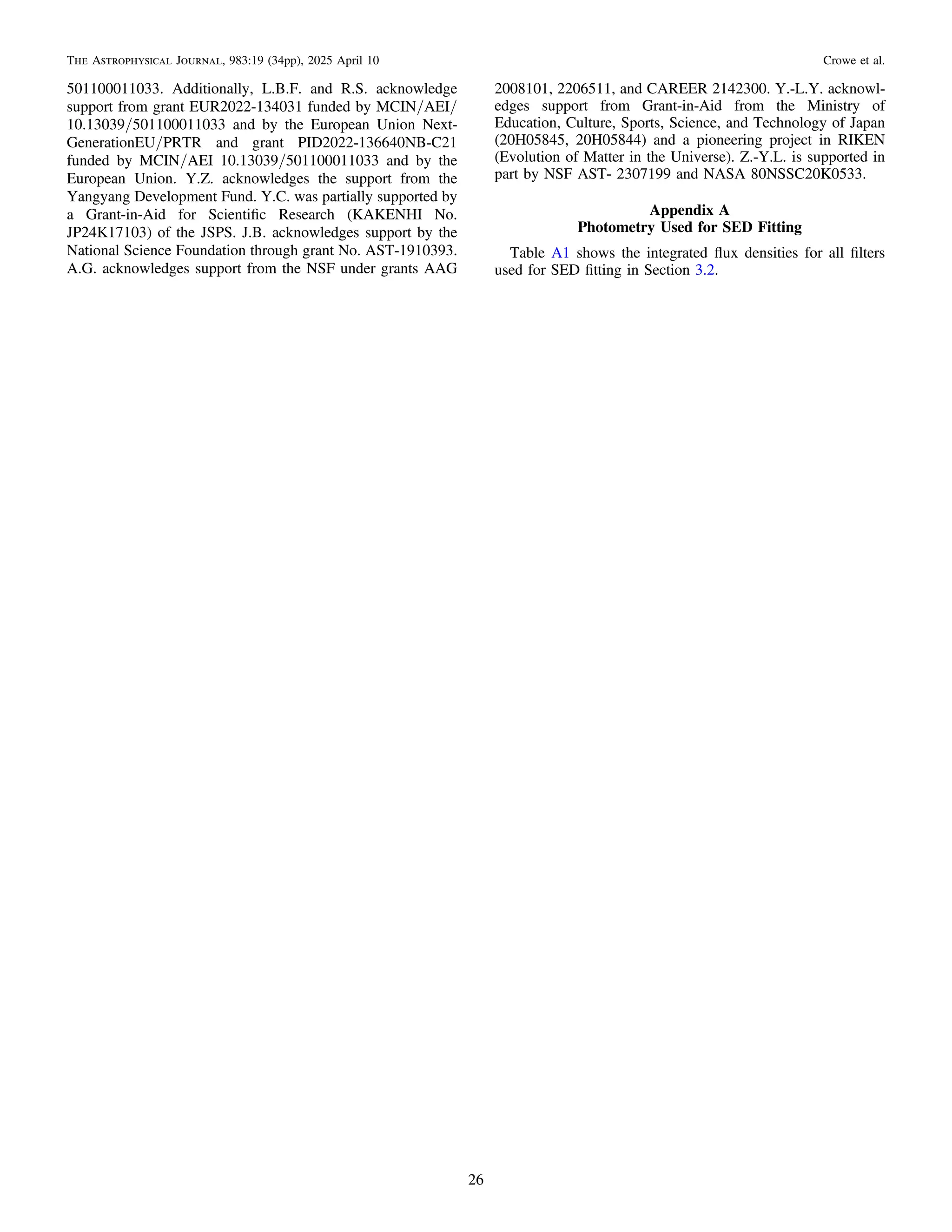
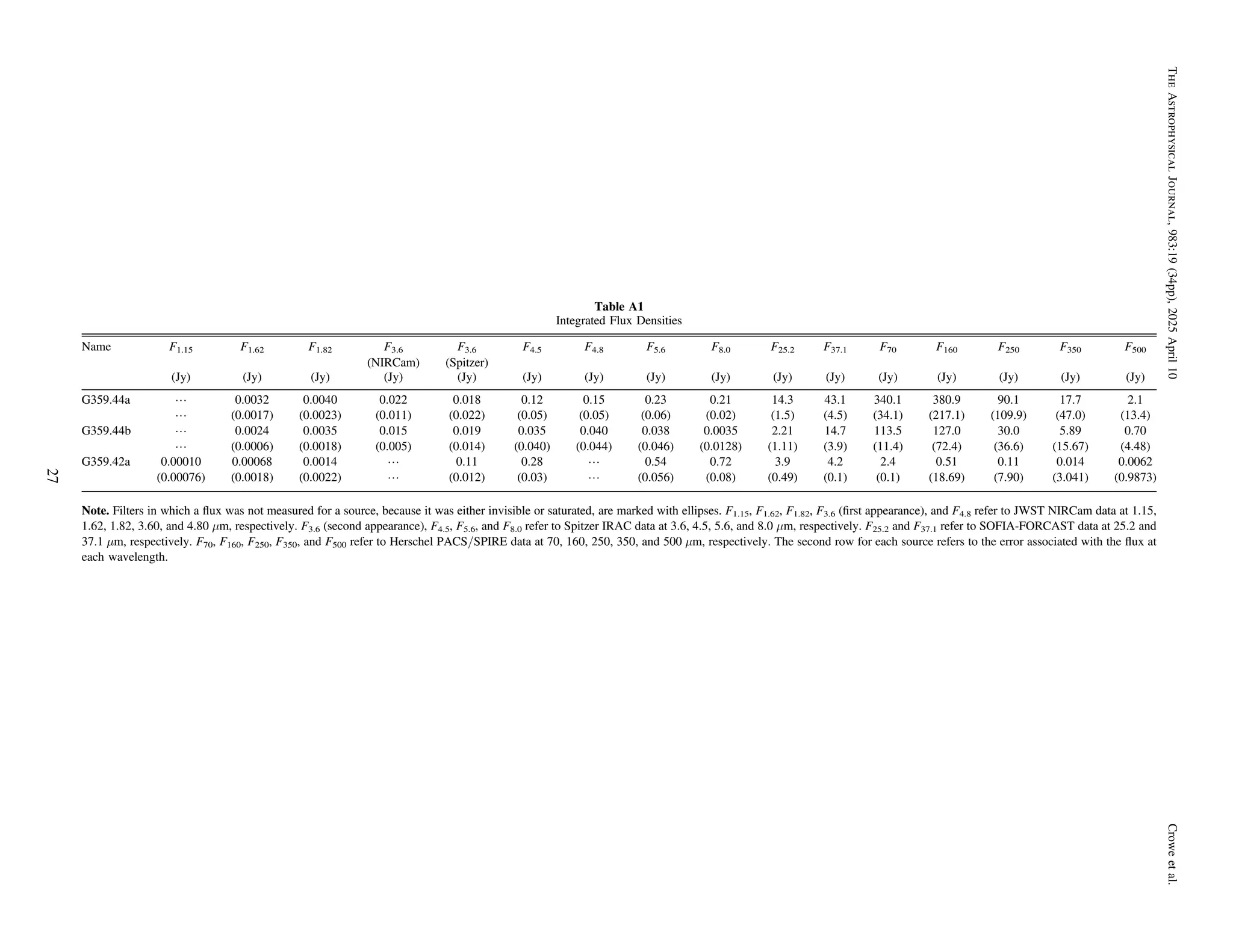
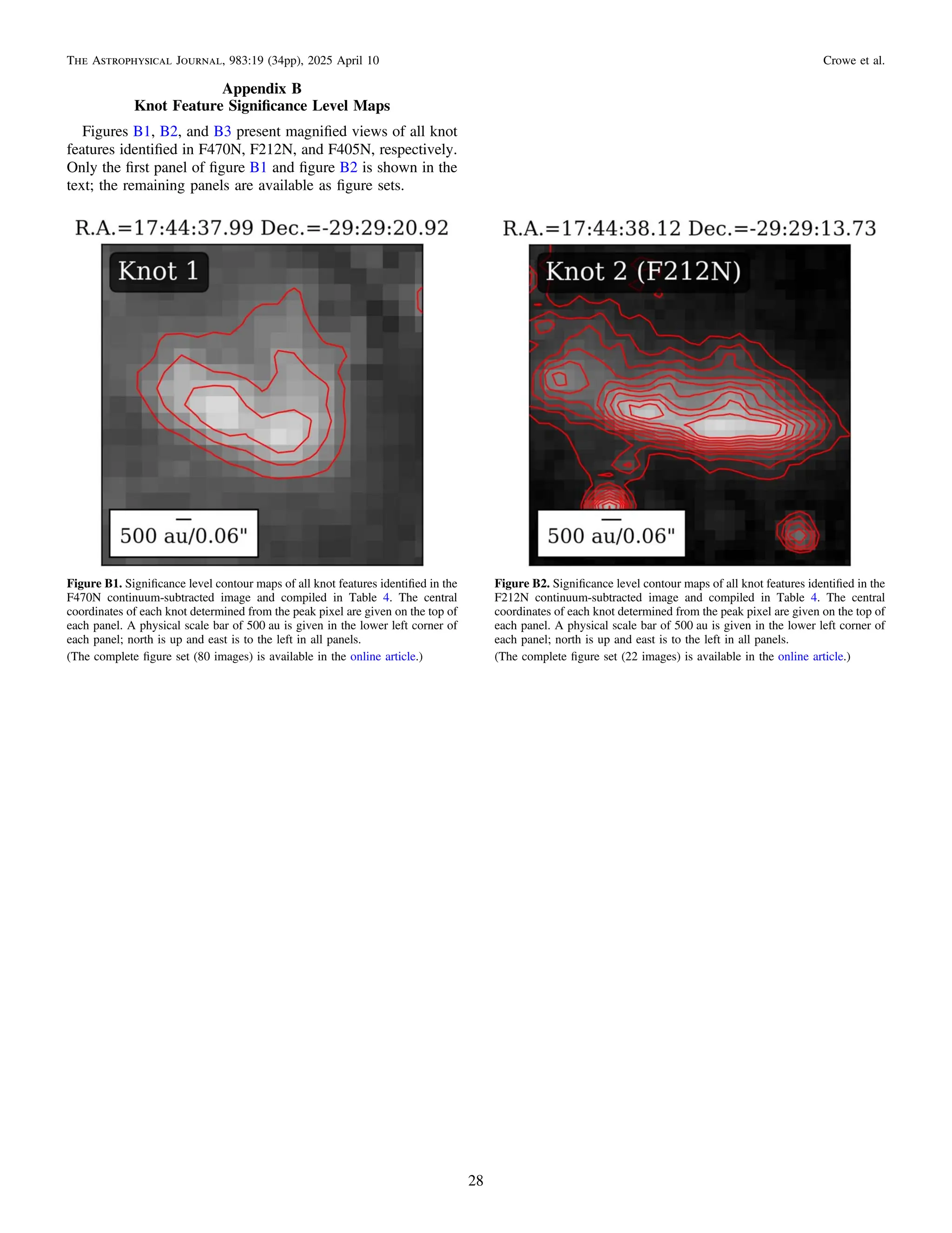
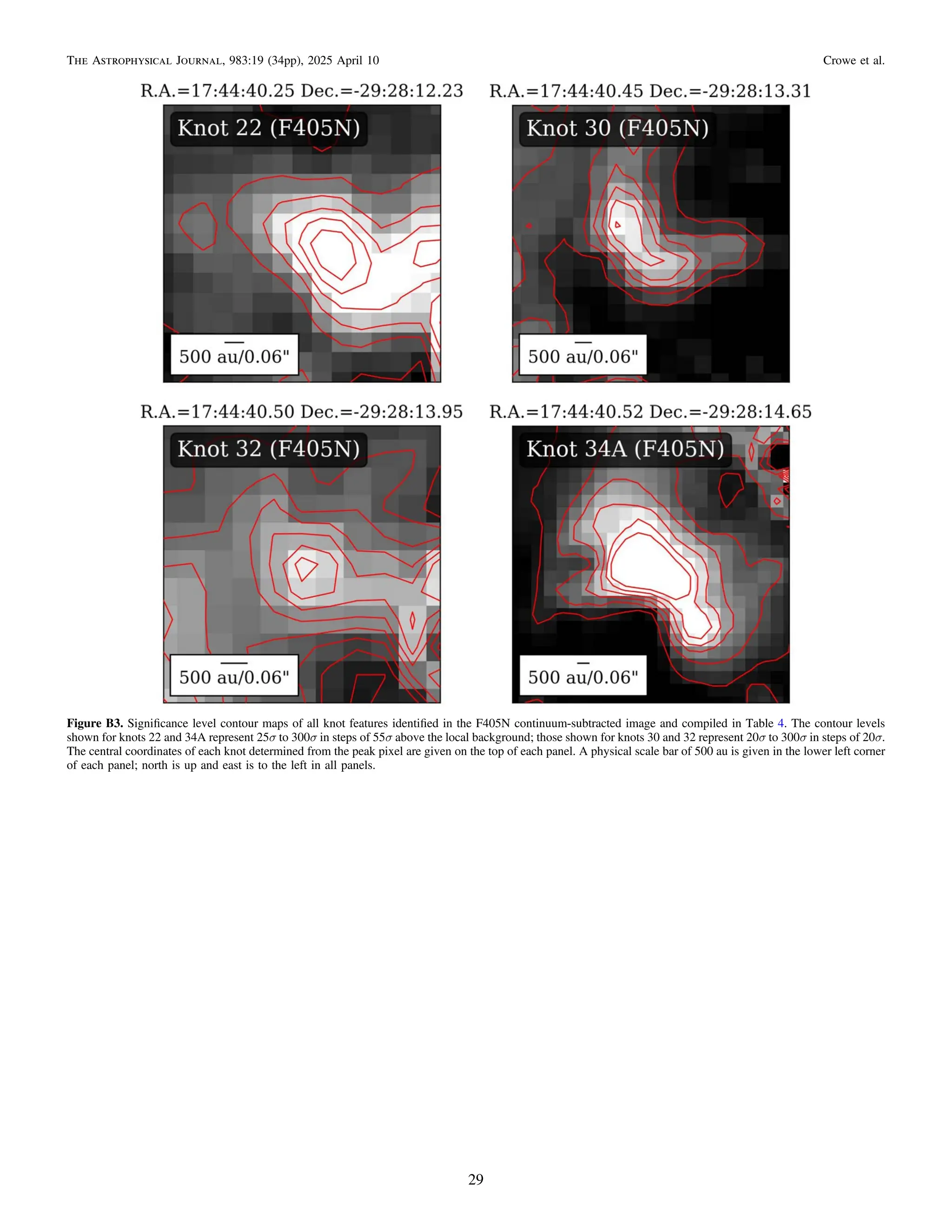
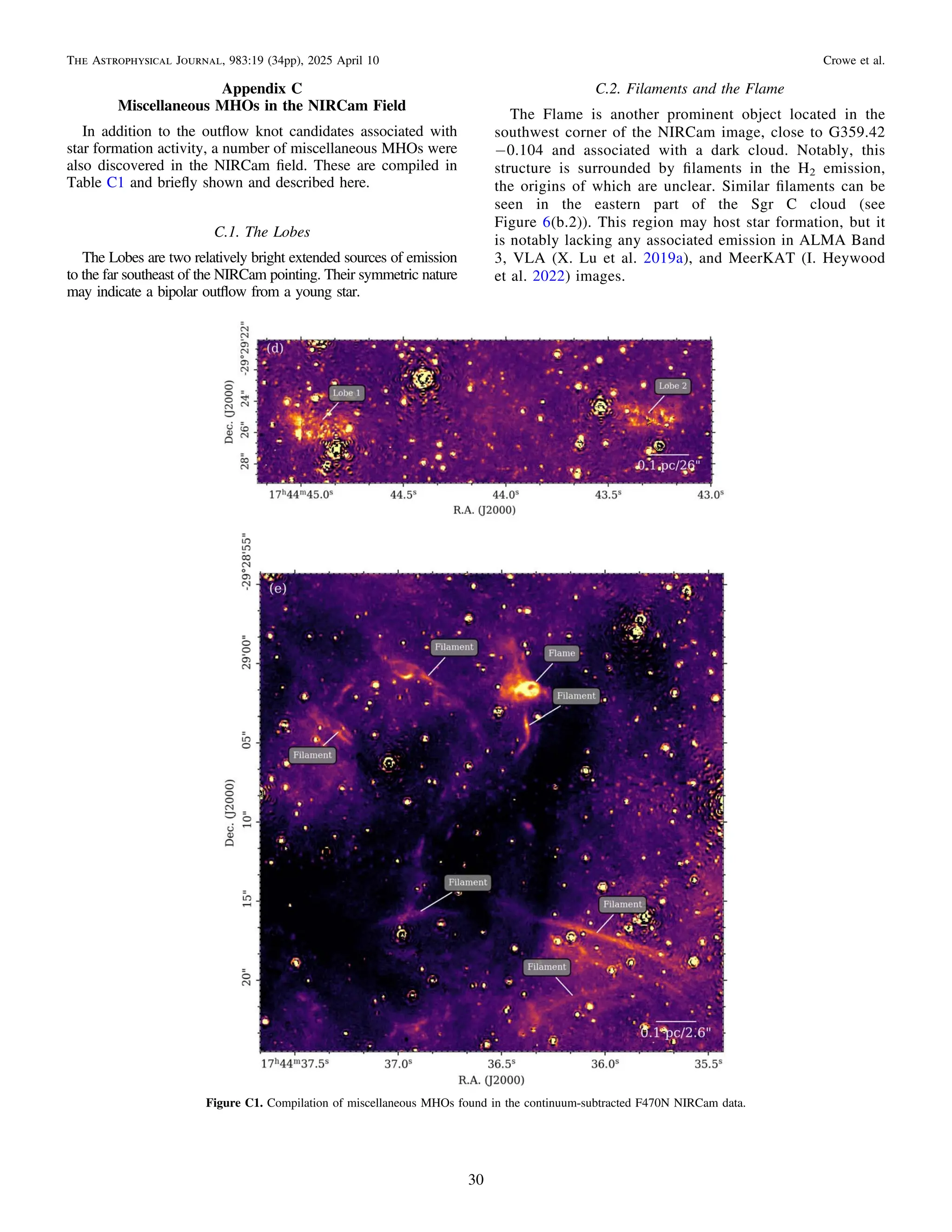
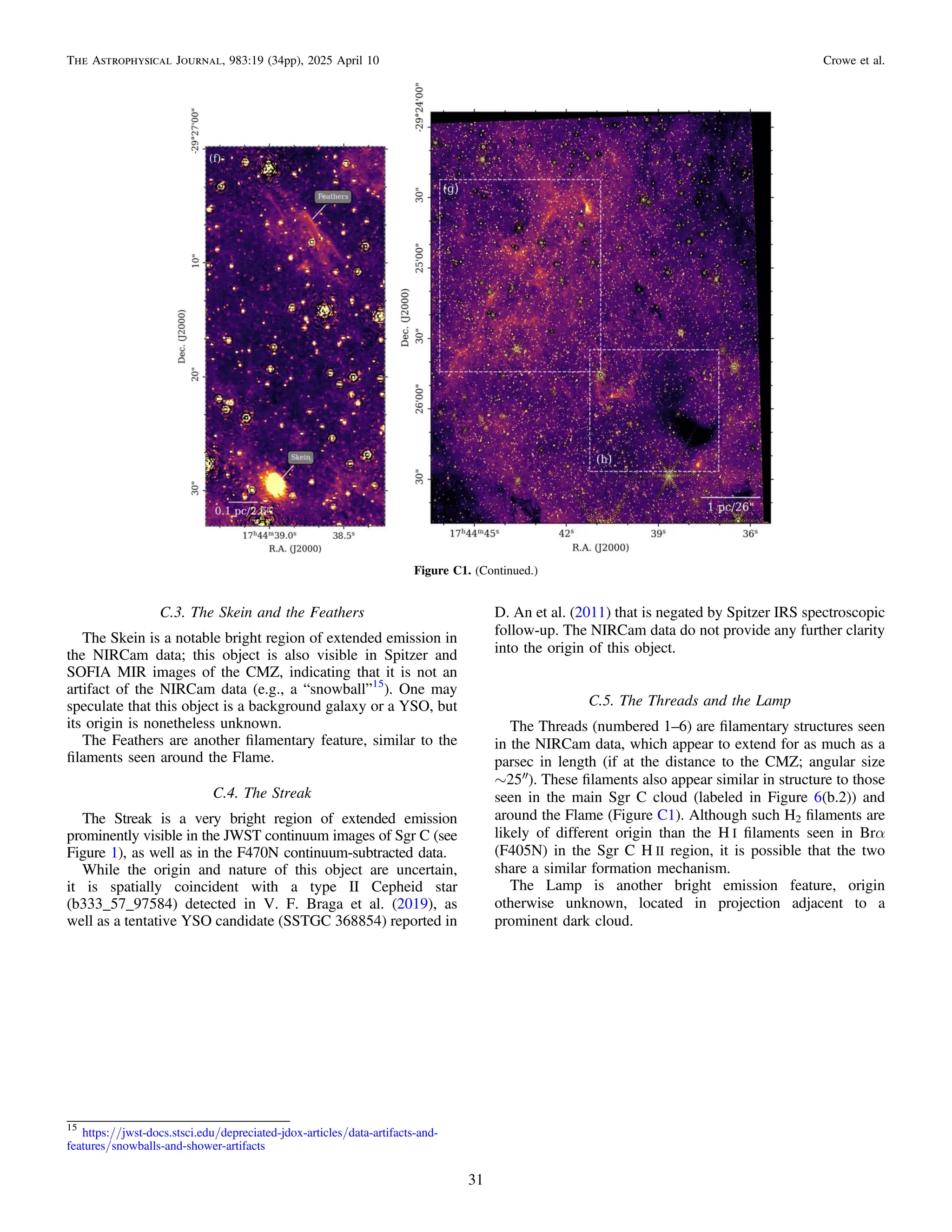
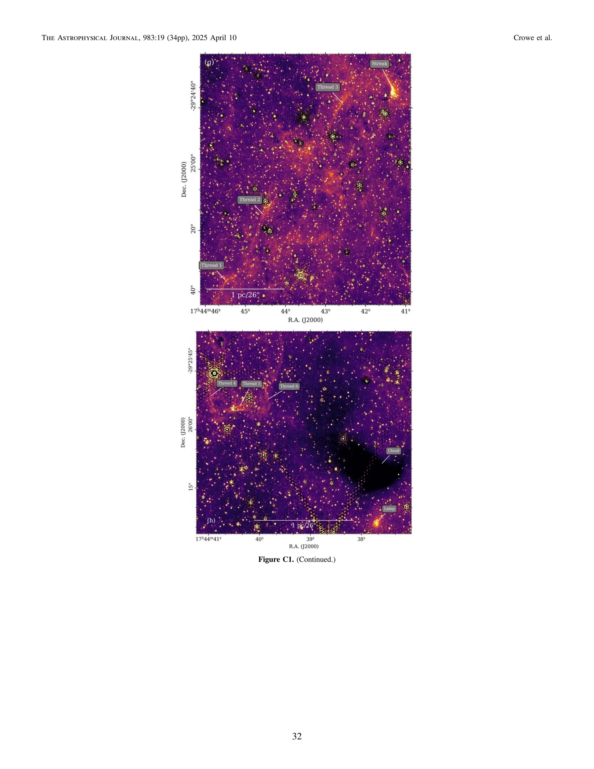
Download to read offline
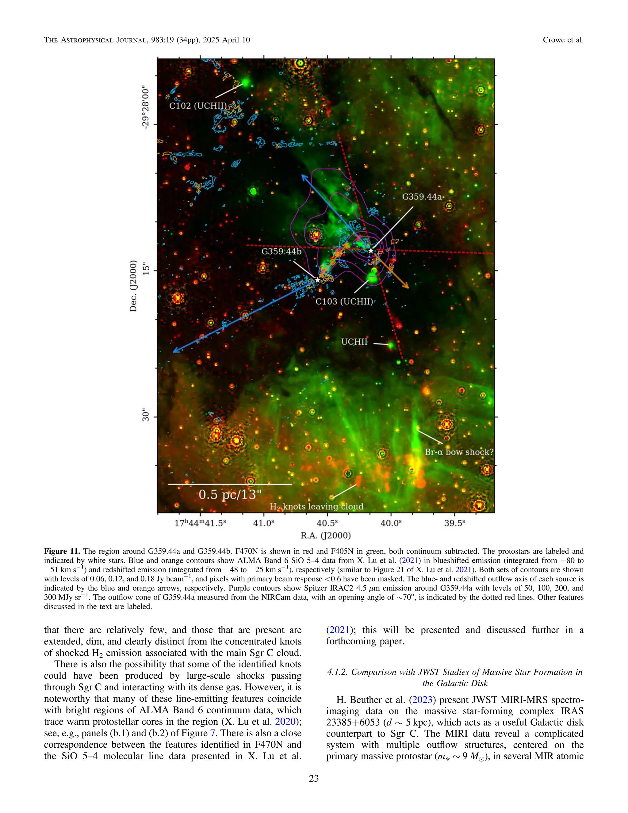
![and molecular lines (H2, [Fe II], [Ne II]). These structures are
corroborated by emission seen in 3.5 mm SiO 2–1 data taken
with the IRAM NOrthern Extended Millimeter Array
(NOEMA). Unlike IRAS 23385+6053, which displays at least
three separate outflow axes centered at its main massive
protostar in MIR 5.511 μm H2(0–0)S(7) emission (see Figure 5
of H. Beuther et al. 2023), Sgr C does not show evidence of
multiple outflow axes for either of its main massive protostars,
G359.44a and G359.44b, particularly in the MIR H2 line filter
F470N. Rather, single outflow axes for both G359.44a and
G359.44b are well-defined in both IR and millimeter lines (see
Figure 11), implying that they are forming relatively unper-
turbed by nearby YSOs, although G359.44a does demonstrate
some indication of precession in its outflow that may have
been caused by dynamical interactions with nearby sources
(Section 4.1.1). This finding is somewhat counterintuitive,
given the extremity of CMZ conditions compared to the
Galactic disk; however, it may indicate that massive star
formation can occur in the CMZ in a largely similar manner to
that in the Galactic disk.
However, as the results of H. Beuther et al. (2023) indicate,
multiple infrared tracers of jet/outflow emission, such as [Fe II]
and [Ne II], which are not included in the present study, are
needed to obtain a full picture of the different components of
outflows in these regions. Additionally, measurements of
accretion/ejection rates, the former of which H. Beuther
et al. (2023) make with the Humphreys α H I(7–6) line at
12.37 μm, and probes of the warm/hot gas content
(∼200–2000 K) in the wider environment can place further
constraint on massive star formation (C. Gieser et al. 2023).
Therefore, high-resolution MIR spectroscopy measurements
with JWST, on G359.44a/b and other CMZ massive protostars
in other clouds (e.g., Sgr B, 50 km s−1
, 20 km s−1
, and the
Brick; see A. Ginsburg et al. 2023, for more information about
the Brick in particular), along with further studies on Galactic
disk massive protostars (from, e.g., the IPA survey; T. Megeath
et al. 2021; S. Federman et al. 2024), will be needed to
construct a proper comparison between massive star formation
in the CMZ and the Galactic disk.
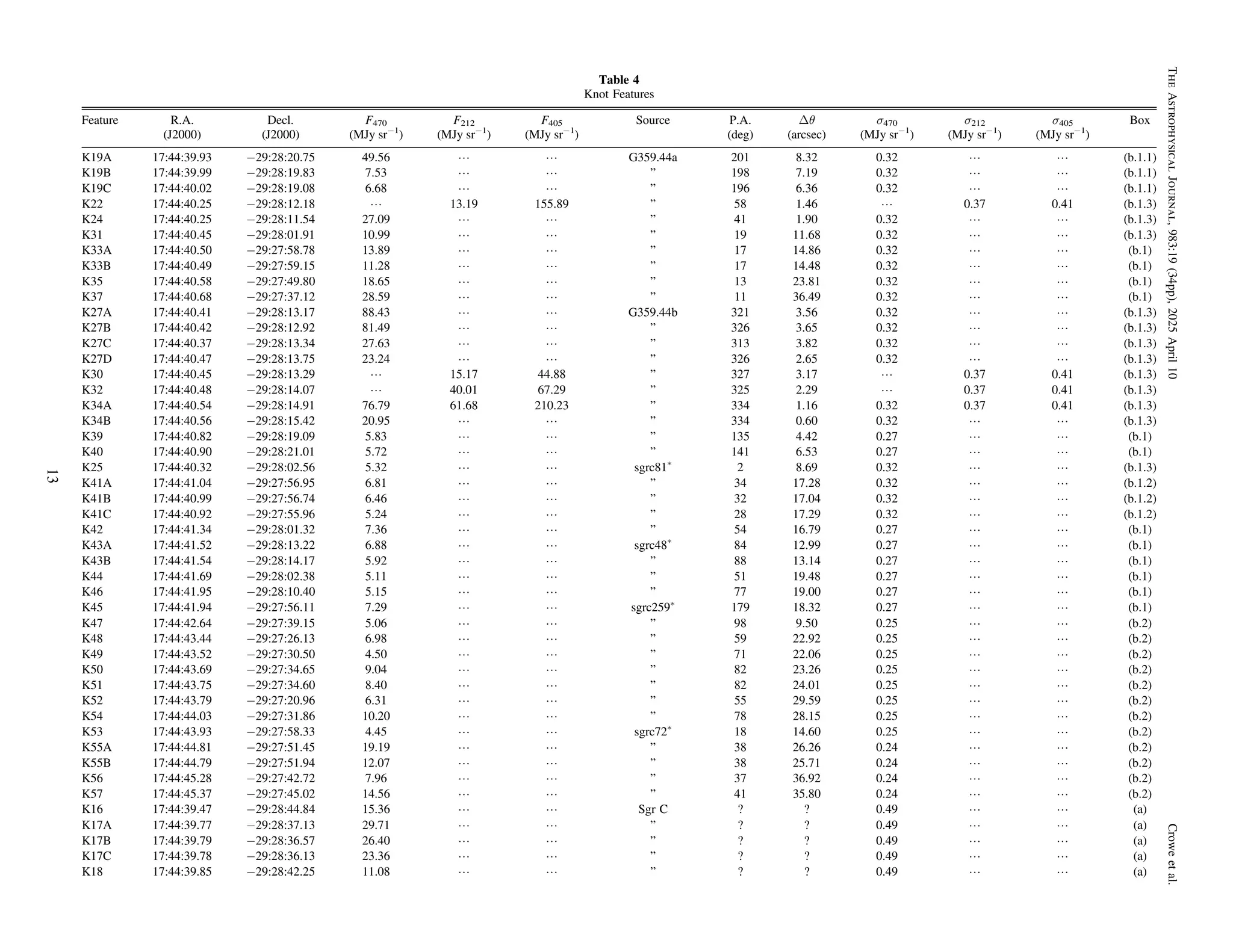
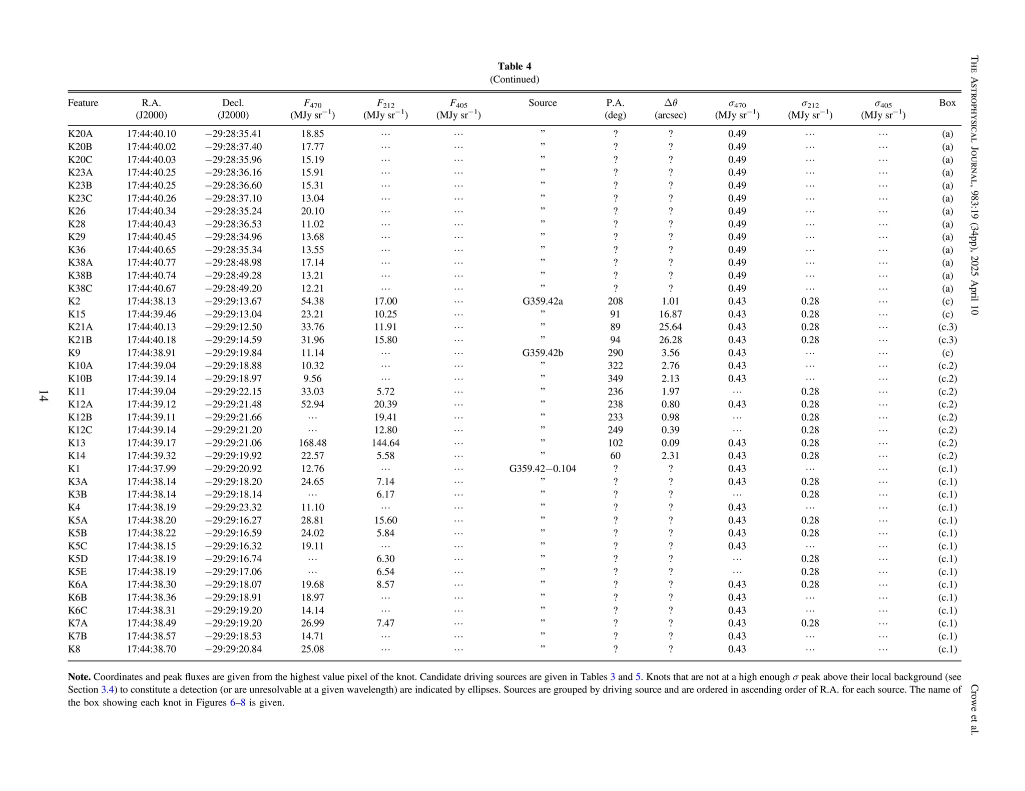
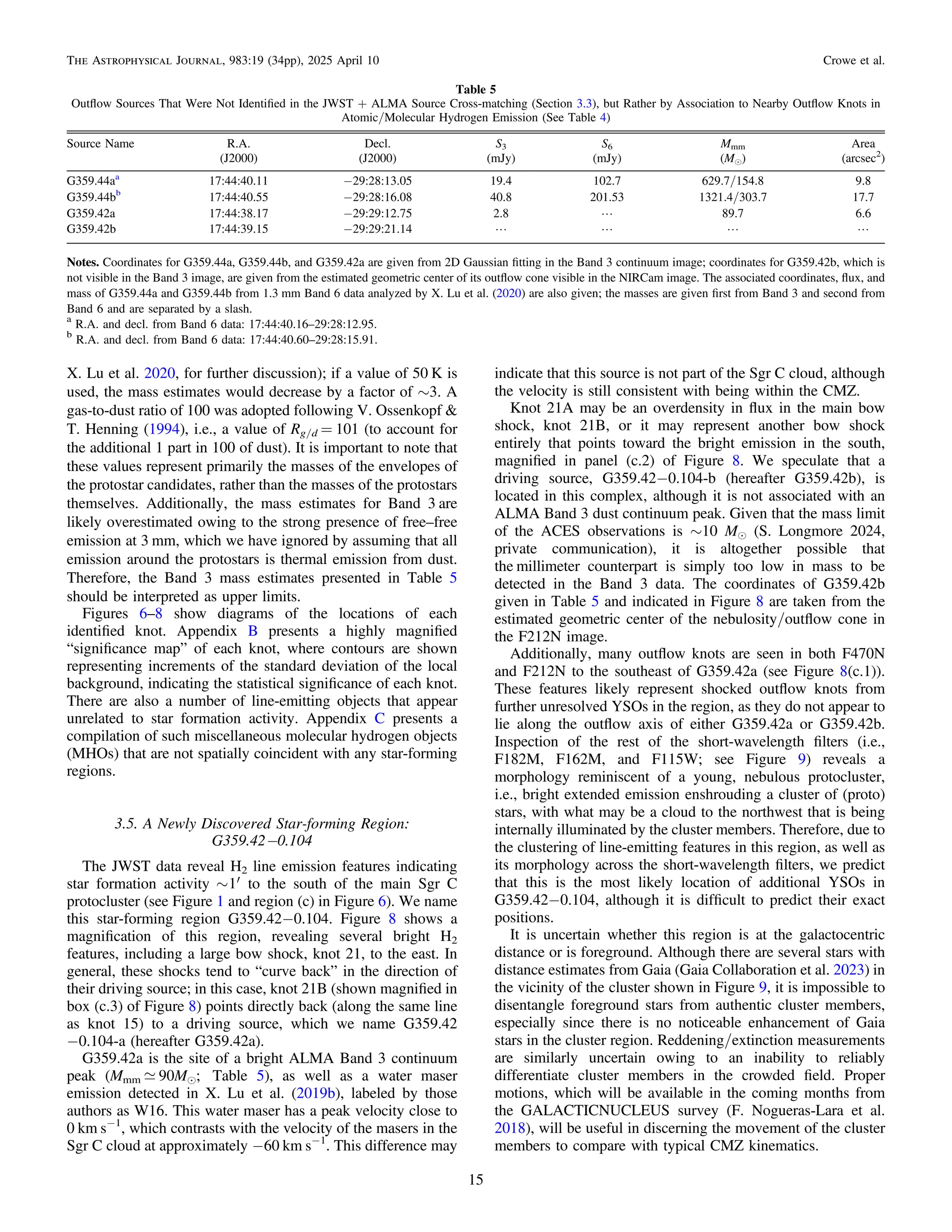
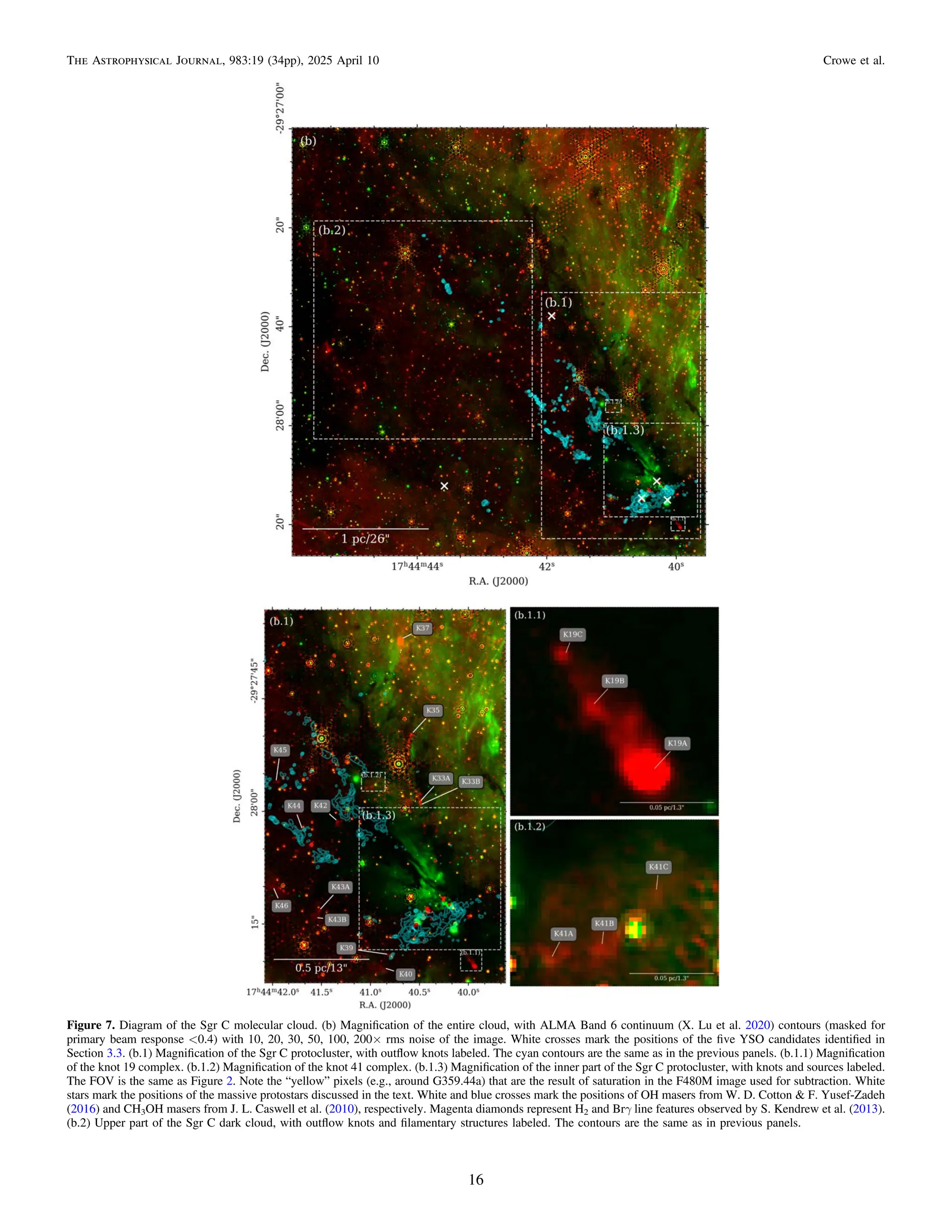
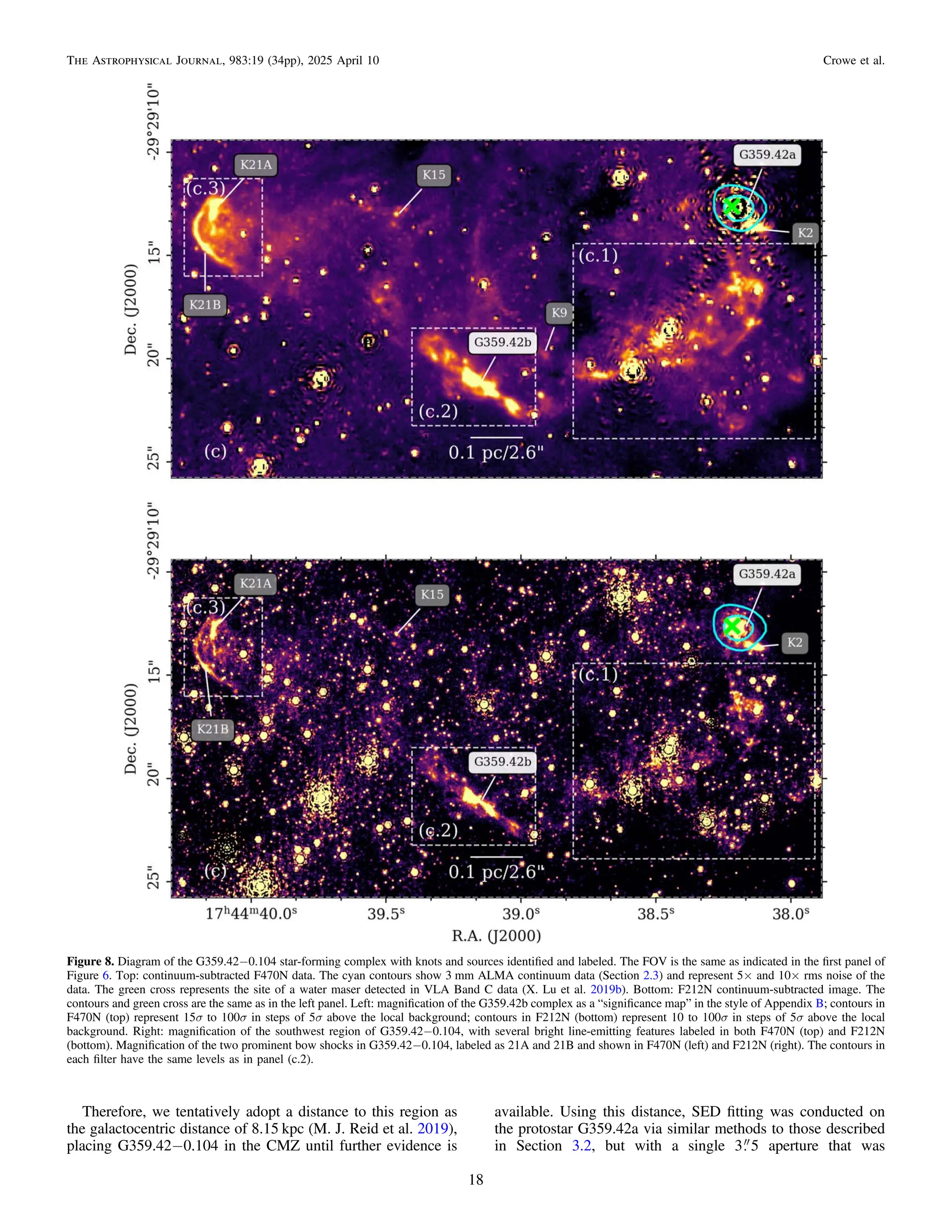
4.1.3. Outflows in G359.42−0.104
Another promising result of analysis of the F470N
continuum-subtracted emission near Sgr C is the discovery
and tentative placement at the galactocentric distance of a new
star-forming region, G359.42−0.104 (Section 3.5). The source
G359.42a, the brightest infrared source in the region, may be a
massive (m* > 8 Me) protostar, with a current stellar mass
predicted by SED fitting of m* ; 9 Me (Table 2). This claim is
supported by its massive associated millimeter core (Mmm ∼
90 Me) and the relatively large luminosity of its associated
water maser, ∼1 × 10⁻⁵
Le (X. Lu et al. 2019b), which implies
massive star formation activity as suggested by the relationship
between H2O maser luminosity and host source luminosity
observed by J. S. Urquhart et al. (2011). It is worth noting,
however, that the trend observed by J. S. Urquhart et al. (2011)
experiences quite a substantial spread and that water masers are
known to vary by orders of magnitude over relatively short
timescales (X. Lu et al. 2019b). The lower bound on the current
stellar mass of G359.42a, m* ; 3.5 Me, is also outside of the
normal mass range for massive protostars (m* > 8 Me) and
would instead be indicative of an intermediate-mass protostar.
Additionally, the SED-fitting derived parameters and
measured millimeter core mass depend heavily on the adopted
distance to the region, which we take to be at the galactocentric
distance of 8.15 kpc, but which may be lower if the region is
foreground to the CMZ. For example, if the distance to
G359.42−0.104 is instead 4 kpc, the SED-fitting derived mass
and millimeter core mass estimate would be m* ; 5 Me and
Mmm ∼ 22 Me, respectively.
A dynamical age estimate can be derived for G359.42a, as
for G359.44a. Assuming a knot velocity of 50–100 km s−1
, and
with an angular separation between the bright bow shock K21B
and G359.42a of ∼26″ and with our adopted distance
to the source of 8.15 kpc, we estimate a dynamical age of
10,000–20,000 yr, placing a lower limit on the age of G359.42a
of ∼104
yr old, depending on its distance.
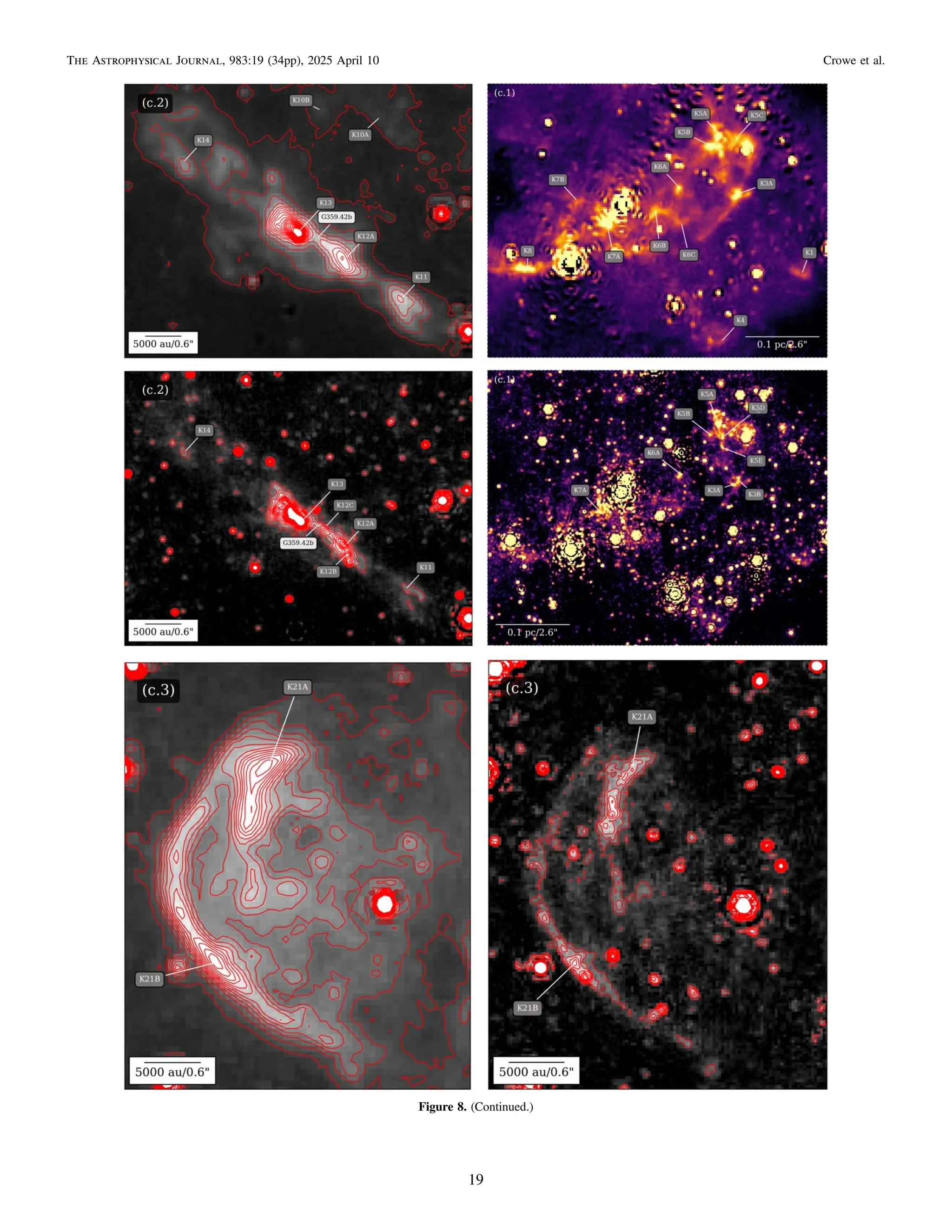
Although G359.42a is the only protostar in G359.42−0.104
associated with both a millimeter core and water maser, there is
evidence for other protostars in the region. We call the most
promising candidate G359.42b, which was identified based on
the distinctive morphology of its surrounding emission (see
Figure 8(c.2)). One of its associated emission-line objects, knot
13, has a morphology reminiscent of an outflow cone
emanating from G359.42b; in this case, we estimate this
outflow cone to have an opening angle of ∼40°. We also note
that some of the outflow knots originating from G359.42b
come in pairs on opposing sides of the source, e.g., knots 14
and 11 (2 31 and 1 97 from G359.42b, respectively). This
may provide an indication of episodic accretion resulting in the
ejection of outflow knots from the source, a phenomenon that
has been previously observed in massive star-forming regions
(e.g., A. Caratti o Garatti et al. 2017; R. Cesaroni et al. 2018;
R. Fedriani et al. 2023a). From end to end, the outflow from
G359.44b appears to be ∼18″ (∼0.7 pc at a distance of
8.15 kpc), including knot 21A.
Ultimately, higher-sensitivity and higher-resolution observa-
tions of G359.42−0.104, especially in the millimeter and
submillimeter, where individual protostellar cores can be
identified and traced back to potential outflow knots, will be
needed to disentangle the full picture of star formation in this
region. Potential relationships with the Sgr C cloud, and
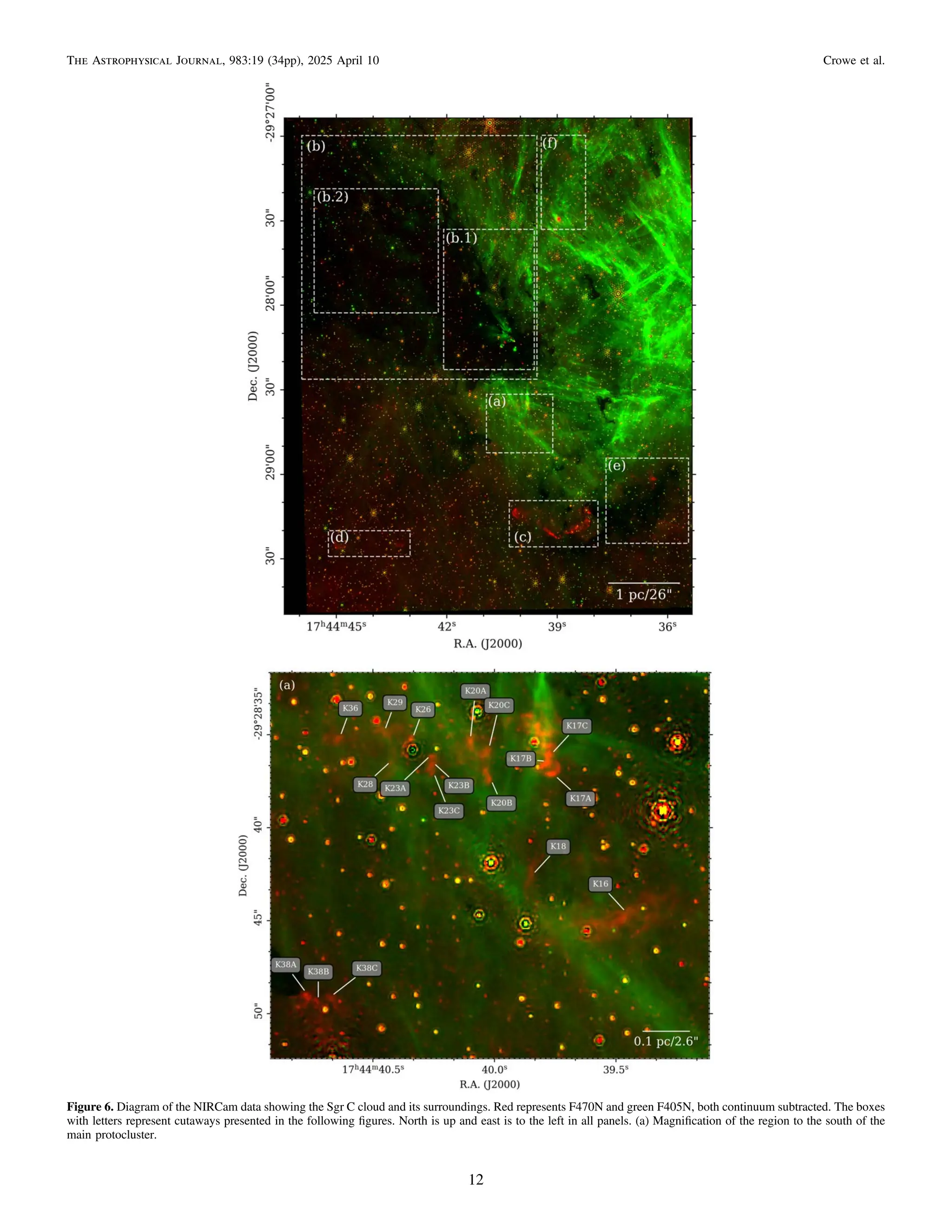
especially with the Sgr C H II region, which is directly adjacent
in projection to G359.42−0.104 (see Figure 6), may also be
revealed with further observations and study of this star-
forming region and its definitive placement at the CMZ
distance (or not) with further data.
4.1.4. Outflows in the CMZ
The first unambiguous detection of protostellar outflows in
the CMZ in the Sgr C cloud and their corroboration directly
with ALMA, presented in this study, have significant
implications for future infrared studies of the CMZ, especially
in the infrared. Infrared observations of the CMZ, particularly
those with the aim of resolving individual protostars and their
associated outflow features, have been historically difficult for
a number of reasons, most notably a lack of resolving power
and the effects of extinction and crowding (F. Nogueras-Lara
et al. 2018, 2019). Studies that attempt to provide comprehen-
sive identification and characterization of CMZ massive
protostars (see, e.g., F. Yusef-Zadeh et al. 2009) have
significant limitations in confirming protostellar detections
and, in turn, constructing a robust catalog. For example,
follow-up studies on the global sample of CMZ massive YSOs
from F. Yusef-Zadeh et al. (2009) prove, using spectroscopic
24
The Astrophysical Journal, 983:19 (34pp), 2025 April 10 Crowe et al.](https://image.slidesharecdn.com/crowe2025apj98319-250407070811-bd3a6242/75/The-JWST-NIRCam-View-of-Sagittarius-C-I-Massive-Star-Formation-and-Protostellar-Outflows-24-2048.jpg)


![and molecular lines (H2, [Fe II], [Ne II]). These structures are
corroborated by emission seen in 3.5 mm SiO 2–1 data taken
with the IRAM NOrthern Extended Millimeter Array
(NOEMA). Unlike IRAS 23385+6053, which displays at least
three separate outflow axes centered at its main massive
protostar in MIR 5.511 μm H2(0–0)S(7) emission (see Figure 5
of H. Beuther et al. 2023), Sgr C does not show evidence of
multiple outflow axes for either of its main massive protostars,
G359.44a and G359.44b, particularly in the MIR H2 line filter
F470N. Rather, single outflow axes for both G359.44a and
G359.44b are well-defined in both IR and millimeter lines (see
Figure 11), implying that they are forming relatively unper-
turbed by nearby YSOs, although G359.44a does demonstrate
some indication of precession in its outflow that may have
been caused by dynamical interactions with nearby sources
(Section 4.1.1). This finding is somewhat counterintuitive,
given the extremity of CMZ conditions compared to the
Galactic disk; however, it may indicate that massive star
formation can occur in the CMZ in a largely similar manner to
that in the Galactic disk.
However, as the results of H. Beuther et al. (2023) indicate,
multiple infrared tracers of jet/outflow emission, such as [Fe II]
and [Ne II], which are not included in the present study, are
needed to obtain a full picture of the different components of
outflows in these regions. Additionally, measurements of
accretion/ejection rates, the former of which H. Beuther
et al. (2023) make with the Humphreys α H I(7–6) line at
12.37 μm, and probes of the warm/hot gas content
(∼200–2000 K) in the wider environment can place further
constraint on massive star formation (C. Gieser et al. 2023).
Therefore, high-resolution MIR spectroscopy measurements
with JWST, on G359.44a/b and other CMZ massive protostars
in other clouds (e.g., Sgr B, 50 km s−1
, 20 km s−1
, and the
Brick; see A. Ginsburg et al. 2023, for more information about
the Brick in particular), along with further studies on Galactic
disk massive protostars (from, e.g., the IPA survey; T. Megeath
et al. 2021; S. Federman et al. 2024), will be needed to
construct a proper comparison between massive star formation
in the CMZ and the Galactic disk.
4.1.3. Outflows in G359.42−0.104
Another promising result of analysis of the F470N
continuum-subtracted emission near Sgr C is the discovery
and tentative placement at the galactocentric distance of a new
star-forming region, G359.42−0.104 (Section 3.5). The source
G359.42a, the brightest infrared source in the region, may be a
massive (m* > 8 Me) protostar, with a current stellar mass
predicted by SED fitting of m* ; 9 Me (Table 2). This claim is
supported by its massive associated millimeter core (Mmm ∼
90 Me) and the relatively large luminosity of its associated
water maser, ∼1 × 10⁻⁵
Le (X. Lu et al. 2019b), which implies
massive star formation activity as suggested by the relationship
between H2O maser luminosity and host source luminosity
observed by J. S. Urquhart et al. (2011). It is worth noting,
however, that the trend observed by J. S. Urquhart et al. (2011)
experiences quite a substantial spread and that water masers are
known to vary by orders of magnitude over relatively short
timescales (X. Lu et al. 2019b). The lower bound on the current
stellar mass of G359.42a, m* ; 3.5 Me, is also outside of the
normal mass range for massive protostars (m* > 8 Me) and
would instead be indicative of an intermediate-mass protostar.
Additionally, the SED-fitting derived parameters and
measured millimeter core mass depend heavily on the adopted
distance to the region, which we take to be at the galactocentric
distance of 8.15 kpc, but which may be lower if the region is
foreground to the CMZ. For example, if the distance to
G359.42−0.104 is instead 4 kpc, the SED-fitting derived mass
and millimeter core mass estimate would be m* ; 5 Me and
Mmm ∼ 22 Me, respectively.
A dynamical age estimate can be derived for G359.42a, as
for G359.44a. Assuming a knot velocity of 50–100 km s−1
, and
with an angular separation between the bright bow shock K21B
and G359.42a of ∼26″ and with our adopted distance
to the source of 8.15 kpc, we estimate a dynamical age of
10,000–20,000 yr, placing a lower limit on the age of G359.42a
of ∼104
yr old, depending on its distance.
Although G359.42a is the only protostar in G359.42−0.104
associated with both a millimeter core and water maser, there is
evidence for other protostars in the region. We call the most
promising candidate G359.42b, which was identified based on
the distinctive morphology of its surrounding emission (see
Figure 8(c.2)). One of its associated emission-line objects, knot
13, has a morphology reminiscent of an outflow cone
emanating from G359.42b; in this case, we estimate this
outflow cone to have an opening angle of ∼40°. We also note
that some of the outflow knots originating from G359.42b
come in pairs on opposing sides of the source, e.g., knots 14
and 11 (2 31 and 1 97 from G359.42b, respectively). This
may provide an indication of episodic accretion resulting in the
ejection of outflow knots from the source, a phenomenon that
has been previously observed in massive star-forming regions
(e.g., A. Caratti o Garatti et al. 2017; R. Cesaroni et al. 2018;
R. Fedriani et al. 2023a). From end to end, the outflow from
G359.44b appears to be ∼18″ (∼0.7 pc at a distance of
8.15 kpc), including knot 21A.
Ultimately, higher-sensitivity and higher-resolution observa-
tions of G359.42−0.104, especially in the millimeter and
submillimeter, where individual protostellar cores can be
identified and traced back to potential outflow knots, will be
needed to disentangle the full picture of star formation in this
region. Potential relationships with the Sgr C cloud, and
especially with the Sgr C H II region, which is directly adjacent
in projection to G359.42−0.104 (see Figure 6), may also be
revealed with further observations and study of this star-
forming region and its definitive placement at the CMZ
distance (or not) with further data.
4.1.4. Outflows in the CMZ
The first unambiguous detection of protostellar outflows in
the CMZ in the Sgr C cloud and their corroboration directly
with ALMA, presented in this study, have significant
implications for future infrared studies of the CMZ, especially
in the infrared. Infrared observations of the CMZ, particularly
those with the aim of resolving individual protostars and their
associated outflow features, have been historically difficult for
a number of reasons, most notably a lack of resolving power
and the effects of extinction and crowding (F. Nogueras-Lara
et al. 2018, 2019). Studies that attempt to provide comprehen-
sive identification and characterization of CMZ massive
protostars (see, e.g., F. Yusef-Zadeh et al. 2009) have
significant limitations in confirming protostellar detections
and, in turn, constructing a robust catalog. For example,
follow-up studies on the global sample of CMZ massive YSOs
from F. Yusef-Zadeh et al. (2009) prove, using spectroscopic
24
The Astrophysical Journal, 983:19 (34pp), 2025 April 10 Crowe et al.](https://crownmelresort.com/image.slidesharecdn.com/crowe2025apj98319-250407070811-bd3a6242/75/The-JWST-NIRCam-View-of-Sagittarius-C-I-Massive-Star-Formation-and-Protostellar-Outflows-24-2048.jpg)


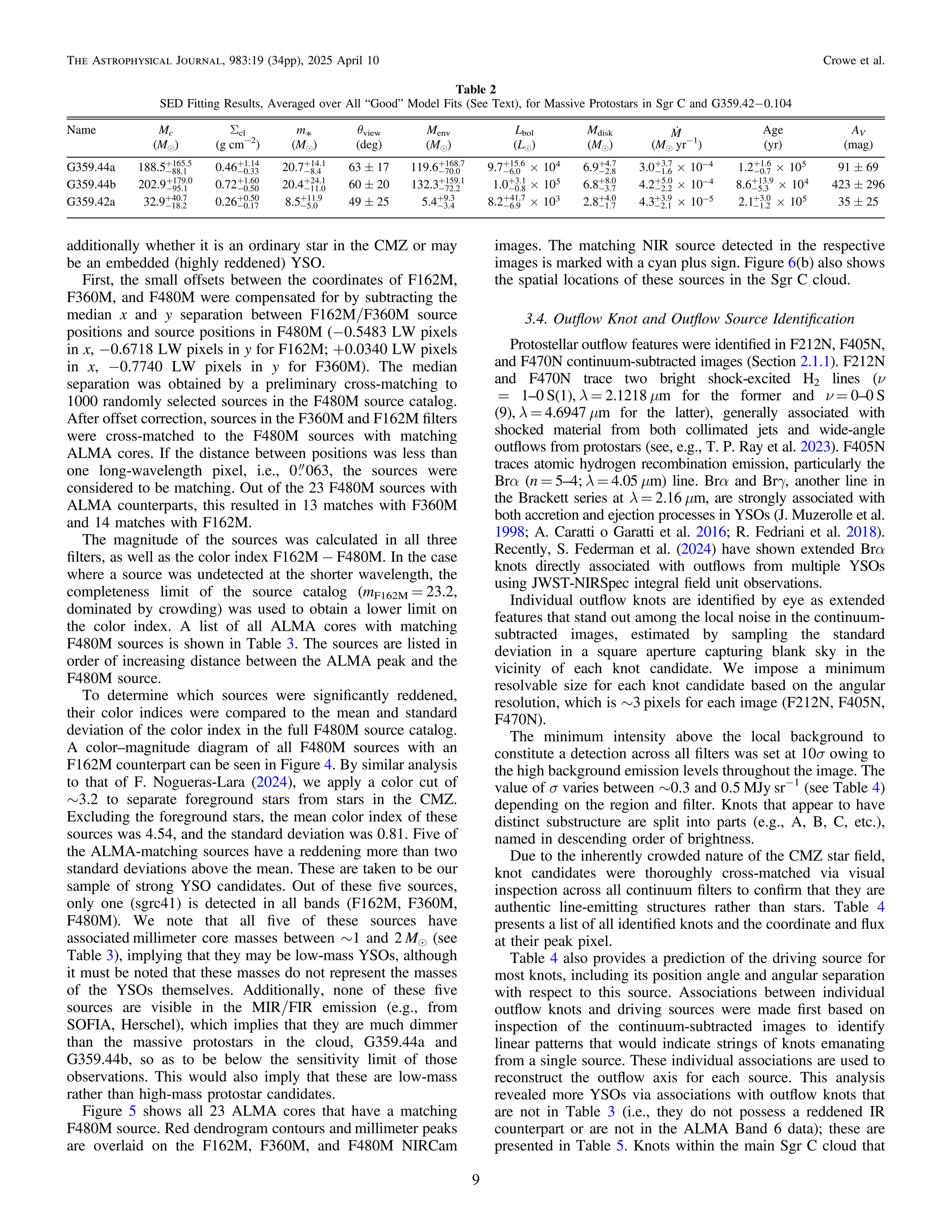
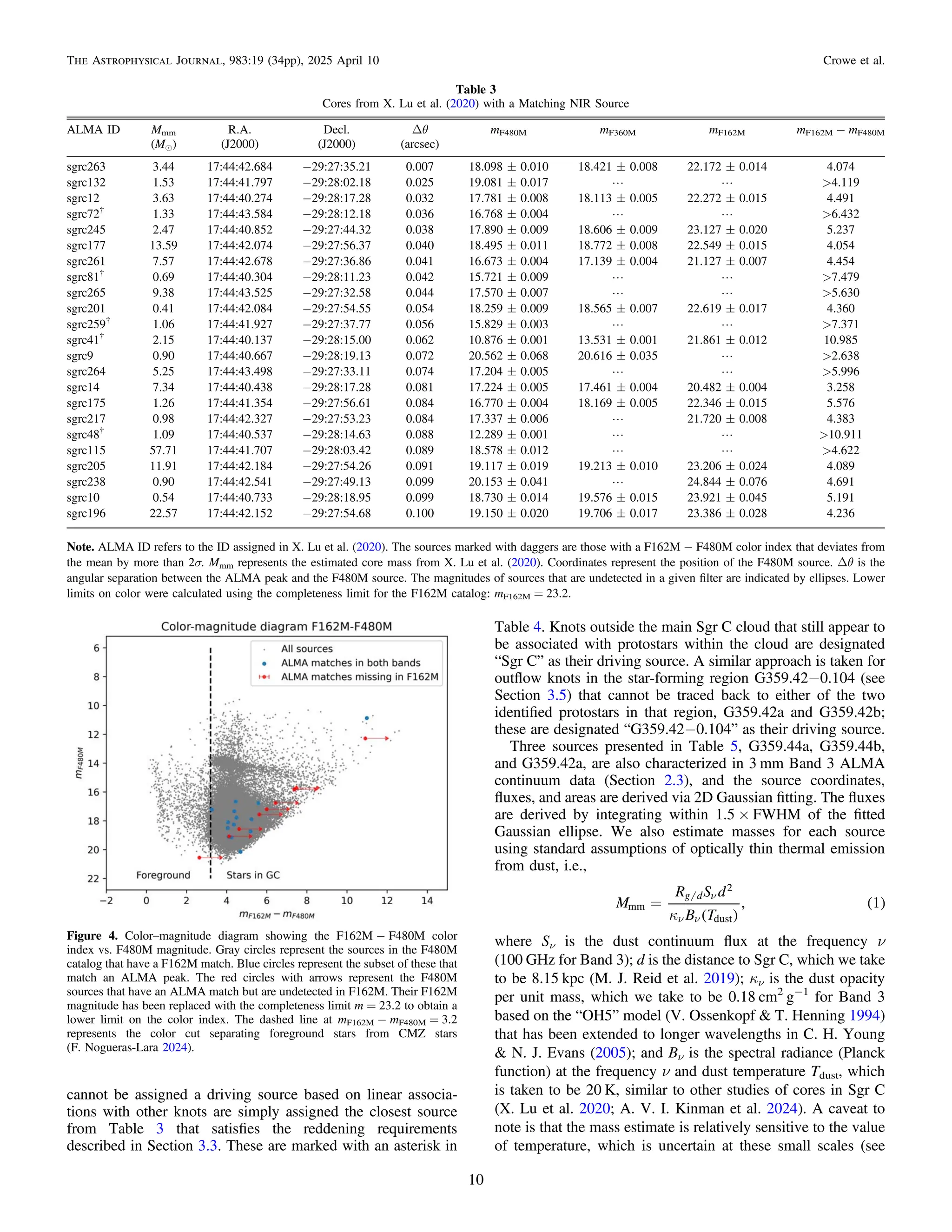
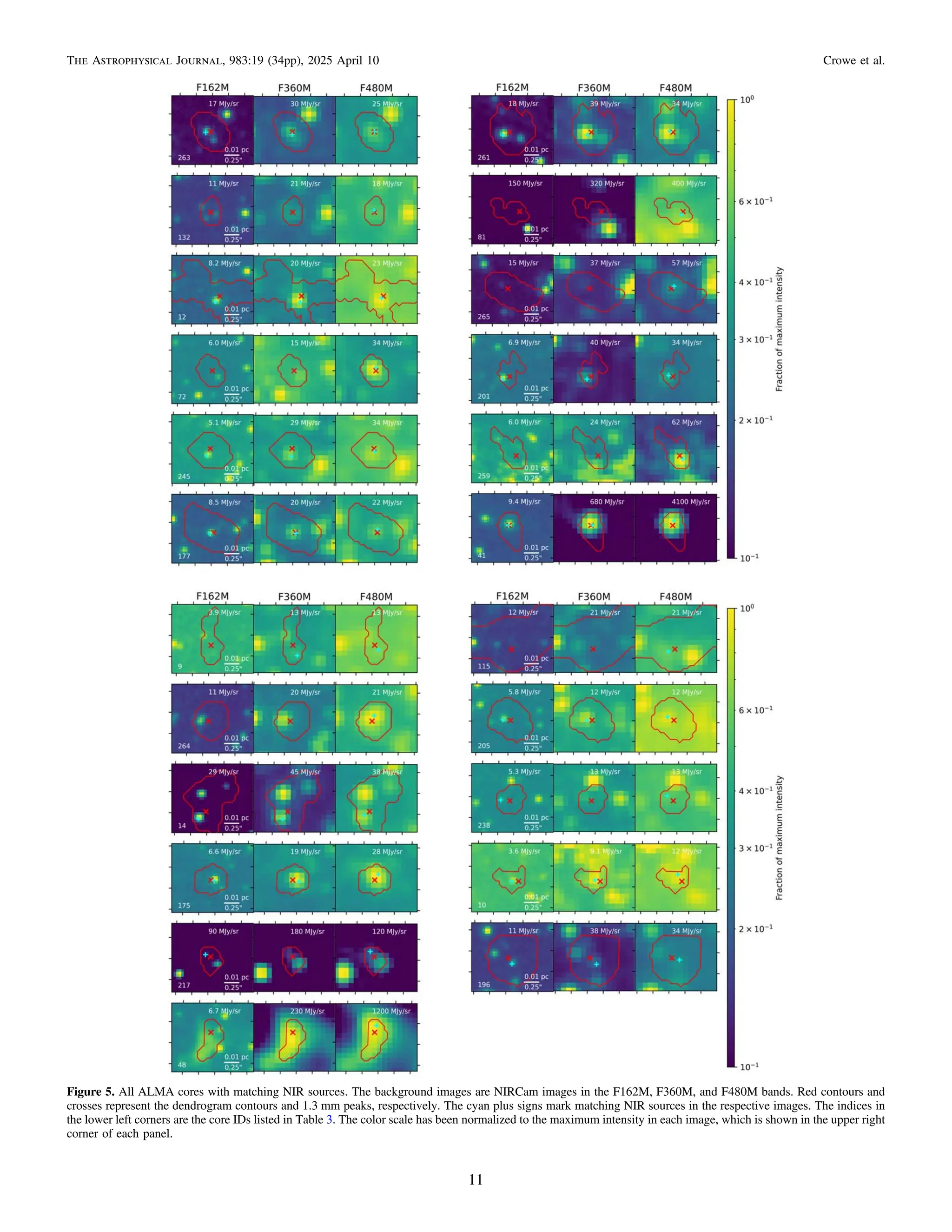
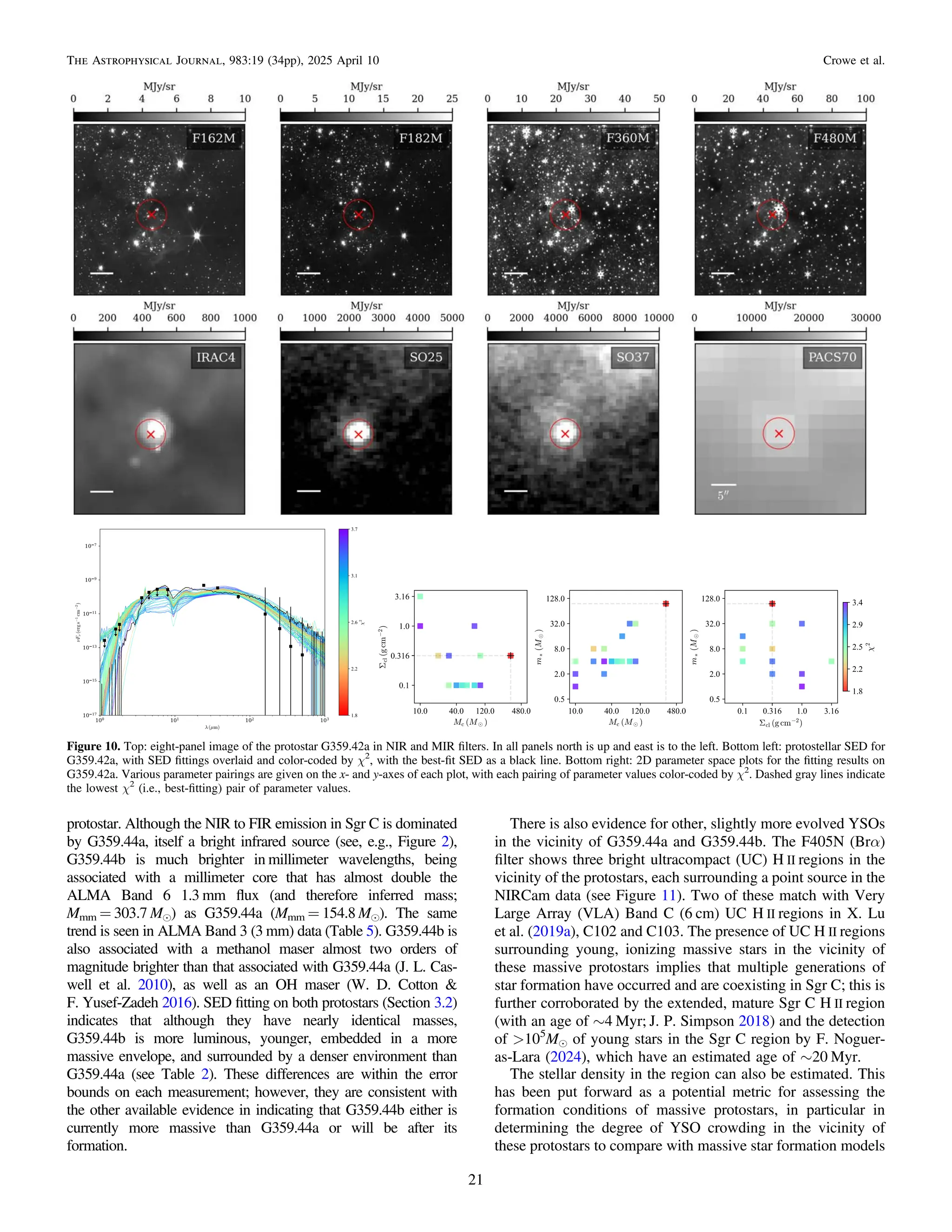
Wepresent James Webb Space Telescope (JWST) Near Infrared Camera observations of the massive star-forming molecular cloud Sagittarius C (Sgr C) in the Central Molecular Zone (CMZ). In conjunction with ancillary mid-IR and far-IR data, we characterize the two most massive protostars in Sgr C via spectral energy distribution (SED) f itting, estimating that they each have current masses of m*∼20Me and surrounding envelope masses of ∼100Me. Wereport a census of lower-mass protostars in Sgr C via a search for infrared counterparts to millimeter continuum dust cores found with the Atacama Large Millimeter/submillimeter Array (ALMA). We identify 88 molecular hydrogen outflow knot candidates originating from outflows from protostars in Sgr C, the first such unambiguous detections in the infrared in the CMZ. About a quarter of these are associated with flows from the two massive protostars in Sgr C; these extend for over 1pc and are associated with outflows detected in ALMA SiO line data. An additional ∼40 features likely trace shocks in outflows powered by lower-mass protostars throughout the cloud. We report the discovery of a new star-forming region hosting two prominent bow shocks and several other line-emitting features driven by at least two protostars. We infer that one of these is forming a highmass star given an SED-derived mass of m*∼9Me and associated massive (∼90Me)millimeter core and water maser. Finally, we identify a population of miscellaneous molecular hydrogen objects that do not appear to be associated with protostellar outflows. Unified Astronomy Thesaurus concepts: Galactic center (565); Massive stars (732); Stellar jets (1607); Star formation (1569); H II regions (694); Stellar bow shocks (1586); Near infrared astronomy (1093); Millimeter astronomy (1061); Spectral energy distribution (2129)


![ALMA Detection of [OIII] 88μmatz=12.33:Exploring the Nature and Evolution of ...](https://cdn.slidesharecdn.com/ss_thumbnails/zavala2024apjl977l9-250125143557-29e4ae2d-thumbnail.jpg?width=640&height=640&fit=bounds)


