Downloaded 51 times

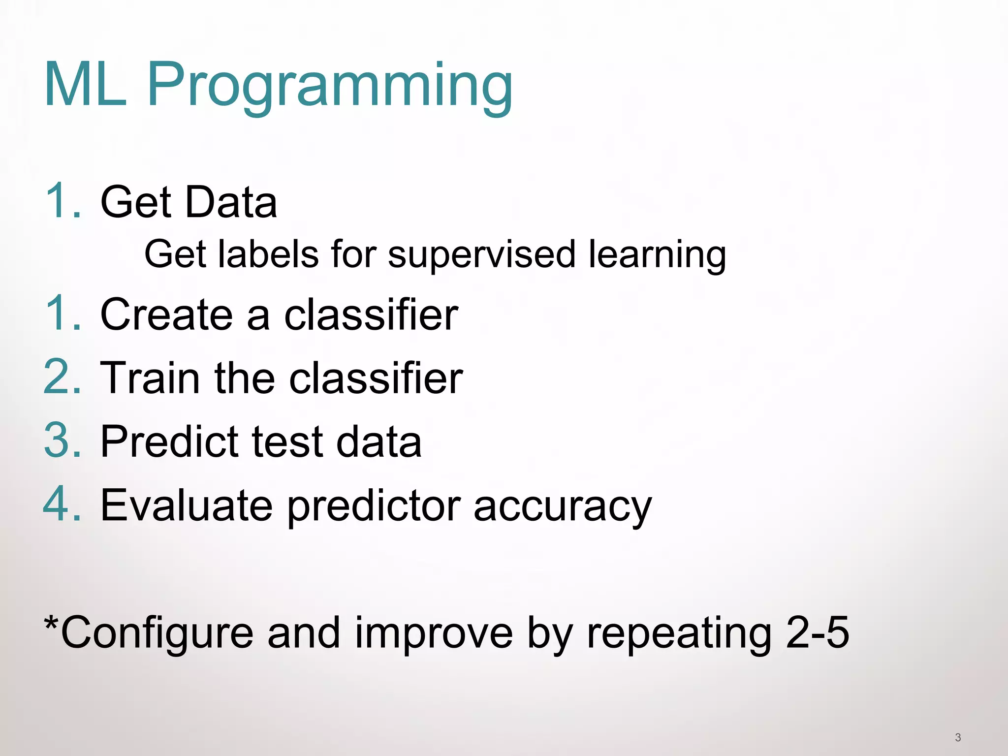
![7
Data Partitioning
• Data and labels
–{[data], [labels]}
–{[3,7, 76, 11, 22, 37, 56,2],[T, T, F, T, F, F, F, T]}
–Data: [Age, Do you love Nutella?]
• Partitioning will create
–{[train data], [train labels],[test data], [test labels]}
–We usually split the data on a ration of 9:1
–There is a tradeoff between the effectiveness of
the test and the learning we could provide to the
classifier
• We will look at a partitioning function later](https://image.slidesharecdn.com/introtomachinelearningwithscikit-learn-150623073429-lva1-app6891/75/Intro-to-machine-learning-with-scikit-learn-7-2048.jpg)


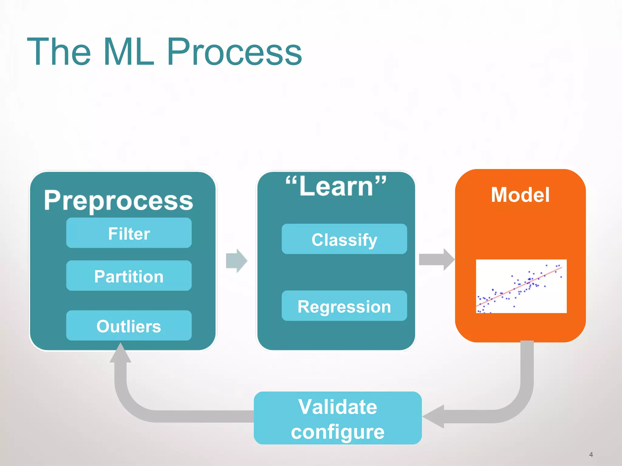
![20
Iris Data
import matplotlib.pyplot as plt
from mpl_toolkits.mplot3d import Axes3D
from sklearn import datasets
iris = datasets.load_iris()
X = iris.data[:, :2] # we only take the first two features.
Y = iris.target
x_min, x_max = X[:, 0].min() - .5, X[:, 0].max() + .5
y_min, y_max = X[:, 1].min() - .5, X[:, 1].max() + .5](https://image.slidesharecdn.com/introtomachinelearningwithscikit-learn-150623073429-lva1-app6891/75/Intro-to-machine-learning-with-scikit-learn-20-2048.jpg)
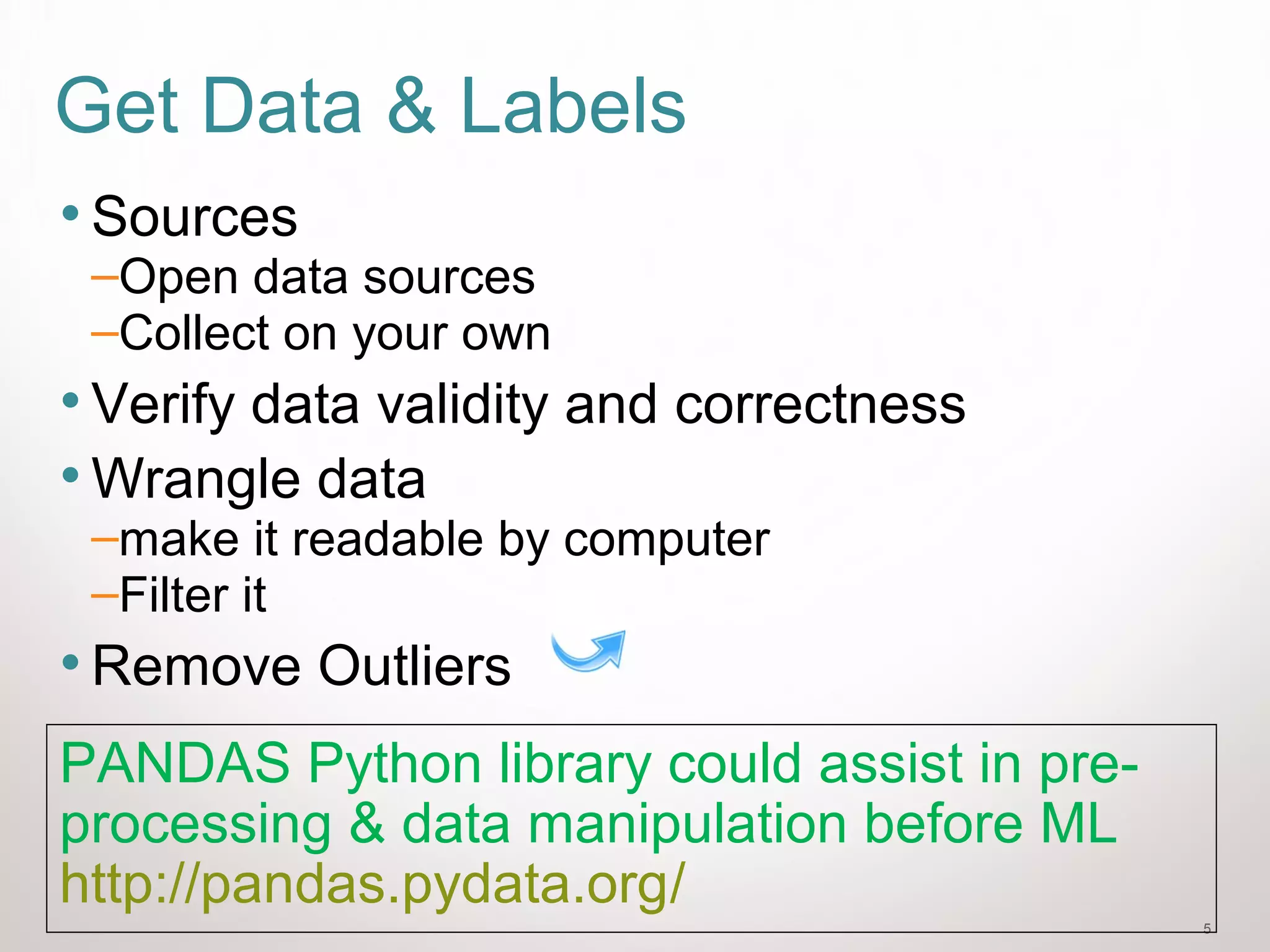
![21
Plot Iris Data
plt.figure(2, figsize=(8, 6))
plt.clf()
plt.scatter(X[:, 0], X[:, 1],
c=Y, cmap=plt.cm.Paired)
plt.xlabel('Sepal length')
plt.ylabel('Sepal width')
plt.xlim(x_min, x_max)
plt.ylim(y_min, y_max)
plt.xticks(())
plt.yticks(())](https://image.slidesharecdn.com/introtomachinelearningwithscikit-learn-150623073429-lva1-app6891/75/Intro-to-machine-learning-with-scikit-learn-21-2048.jpg)
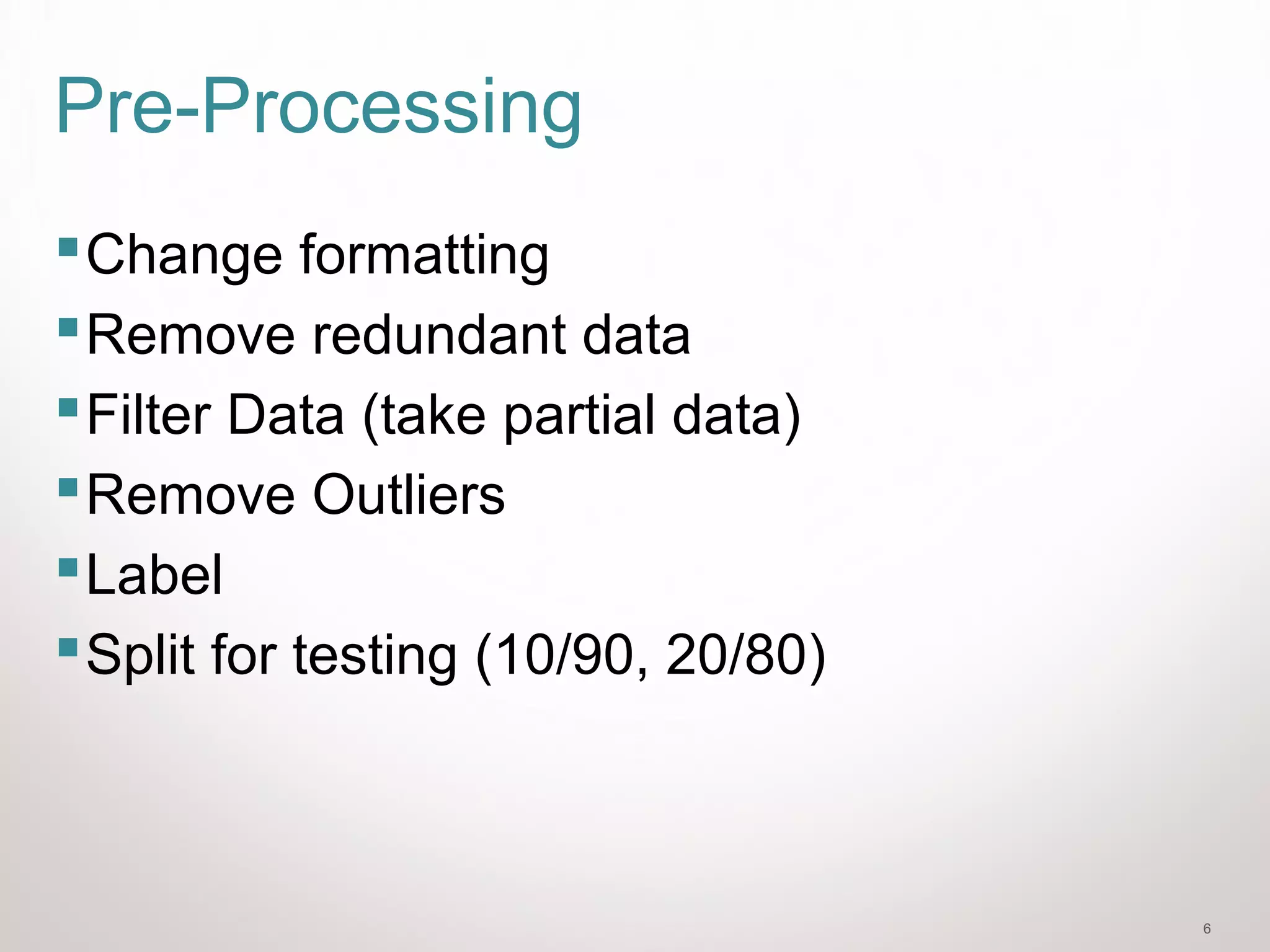
![22
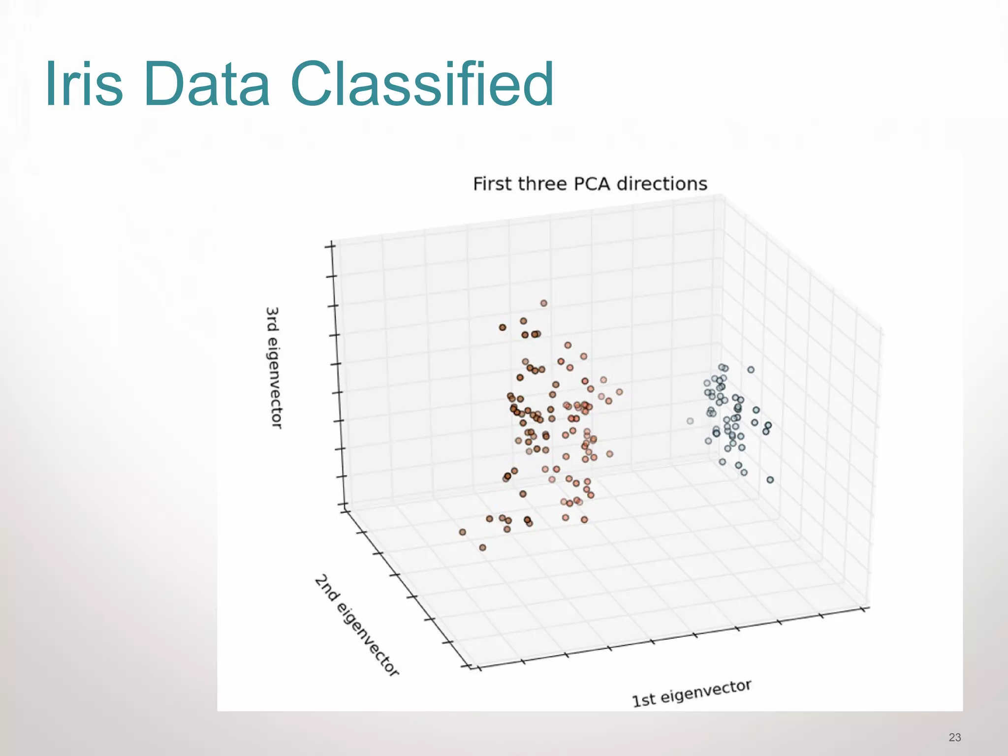
Add PCA for better classification
fig = plt.figure(1, figsize=(8, 6))
ax = Axes3D(fig, elev=-150, azim=110)
X_reduced = PCA(n_components=3).fit_transform(iris.data)
ax.scatter(X_reduced[:, 0], X_reduced[:, 1], X_reduced[:, 2], c=Y,
cmap=plt.cm.Paired)
ax.set_title("First three PCA directions")
ax.set_xlabel("1st eigenvector")
ax.w_xaxis.set_ticklabels([])
ax.set_ylabel("2nd eigenvector")
ax.w_yaxis.set_ticklabels([])
ax.set_zlabel("3rd eigenvector")
ax.w_zaxis.set_ticklabels([])
plt.show()](https://image.slidesharecdn.com/introtomachinelearningwithscikit-learn-150623073429-lva1-app6891/75/Intro-to-machine-learning-with-scikit-learn-22-2048.jpg)


![7
Data Partitioning
• Data and labels
–{[data], [labels]}
–{[3,7, 76, 11, 22, 37, 56,2],[T, T, F, T, F, F, F, T]}
–Data: [Age, Do you love Nutella?]
• Partitioning will create
–{[train data], [train labels],[test data], [test labels]}
–We usually split the data on a ration of 9:1
–There is a tradeoff between the effectiveness of
the test and the learning we could provide to the
classifier
• We will look at a partitioning function later](https://crownmelresort.com/image.slidesharecdn.com/introtomachinelearningwithscikit-learn-150623073429-lva1-app6891/75/Intro-to-machine-learning-with-scikit-learn-7-2048.jpg)


![20
Iris Data
import matplotlib.pyplot as plt
from mpl_toolkits.mplot3d import Axes3D
from sklearn import datasets
iris = datasets.load_iris()
X = iris.data[:, :2] # we only take the first two features.
Y = iris.target
x_min, x_max = X[:, 0].min() - .5, X[:, 0].max() + .5
y_min, y_max = X[:, 1].min() - .5, X[:, 1].max() + .5](https://crownmelresort.com/image.slidesharecdn.com/introtomachinelearningwithscikit-learn-150623073429-lva1-app6891/75/Intro-to-machine-learning-with-scikit-learn-20-2048.jpg)
![21
Plot Iris Data
plt.figure(2, figsize=(8, 6))
plt.clf()
plt.scatter(X[:, 0], X[:, 1],
c=Y, cmap=plt.cm.Paired)
plt.xlabel('Sepal length')
plt.ylabel('Sepal width')
plt.xlim(x_min, x_max)
plt.ylim(y_min, y_max)
plt.xticks(())
plt.yticks(())](https://crownmelresort.com/image.slidesharecdn.com/introtomachinelearningwithscikit-learn-150623073429-lva1-app6891/75/Intro-to-machine-learning-with-scikit-learn-21-2048.jpg)
![22
Add PCA for better classification
fig = plt.figure(1, figsize=(8, 6))
ax = Axes3D(fig, elev=-150, azim=110)
X_reduced = PCA(n_components=3).fit_transform(iris.data)
ax.scatter(X_reduced[:, 0], X_reduced[:, 1], X_reduced[:, 2], c=Y,
cmap=plt.cm.Paired)
ax.set_title("First three PCA directions")
ax.set_xlabel("1st eigenvector")
ax.w_xaxis.set_ticklabels([])
ax.set_ylabel("2nd eigenvector")
ax.w_yaxis.set_ticklabels([])
ax.set_zlabel("3rd eigenvector")
ax.w_zaxis.set_ticklabels([])
plt.show()](https://crownmelresort.com/image.slidesharecdn.com/introtomachinelearningwithscikit-learn-150623073429-lva1-app6891/75/Intro-to-machine-learning-with-scikit-learn-22-2048.jpg)


The document discusses machine learning concepts and programming with scikit-learn. It introduces the machine learning process of getting data, pre-processing, partitioning for training and testing, creating a classifier, training and evaluating the model. As an example, it loads the Iris dataset and plots sepal length vs width with labels. It also uses PCA for dimensionality reduction to better classify the Iris data in 3 dimensions.