Downloaded 49 times

![3
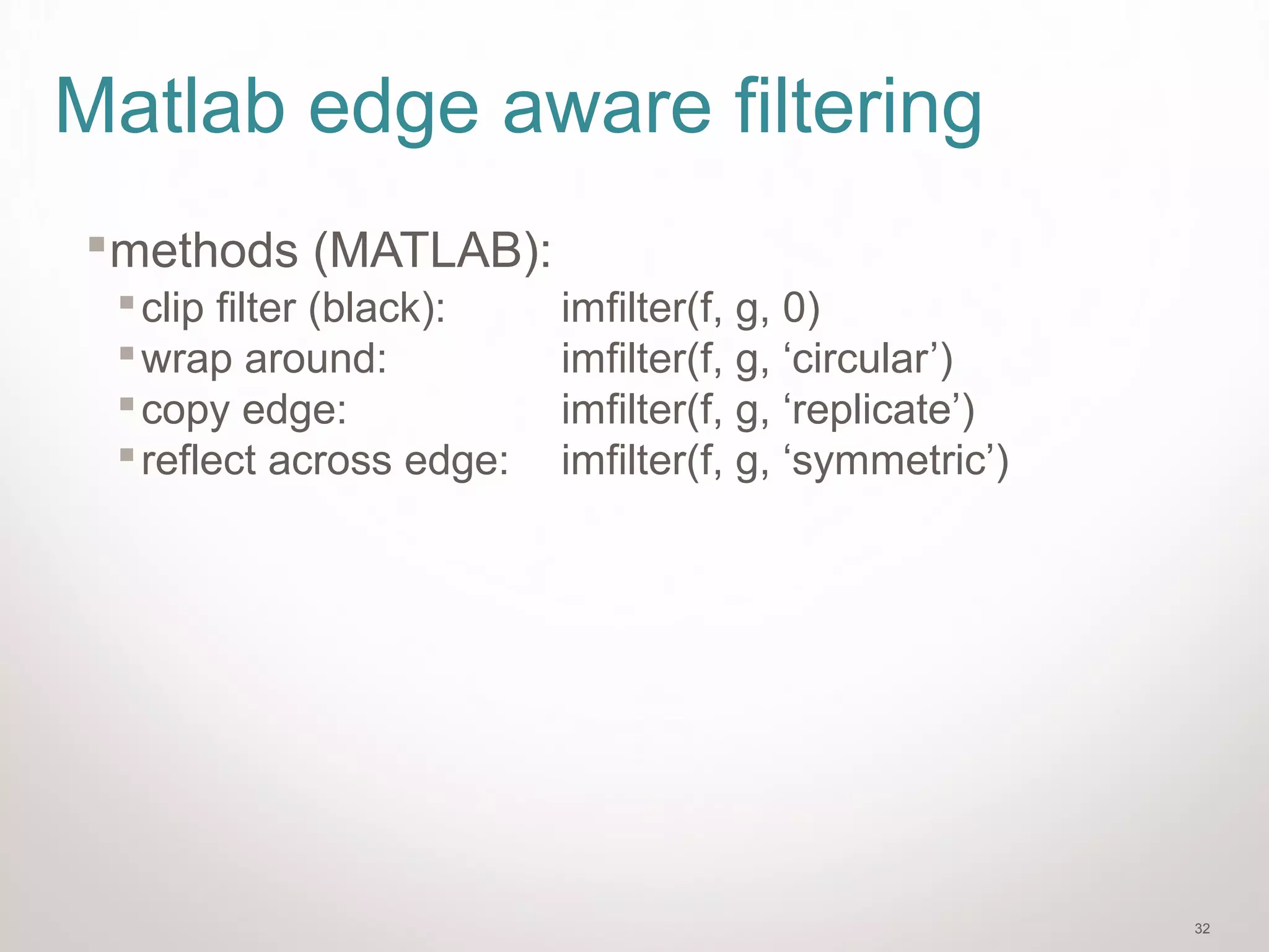
How to filter
2d Correlation
h=filter2(g,f); or h=imfilter(f,g);
2d Convolution
h=conv2(g,f);
],[],[],[
,
lnkmflkgnmh
lk
−−= ∑
f=image
g=filter
],[],[],[
,
lnkmflkgnmh
lk
++= ∑](https://image.slidesharecdn.com/2filters-170112120805/75/Computer-Vision-Image-Filters-3-2048.jpg)
![4
Correlation filtering
Say the averaging window size is 2k+1 x 2k+1:
Loop over all pixels in neighborhood around
image pixel F[i,j]
Attribute uniform
weight to each pixel
Now generalize to allow different weights depending on
neighboring pixel’s relative position:
Non-uniform weights](https://image.slidesharecdn.com/2filters-170112120805/75/Computer-Vision-Image-Filters-4-2048.jpg)
![5
Correlation filtering
Filtering an image: replace each pixel with a linear
combination of its neighbors.
The filter “kernel” or “mask” H[u,v] is the prescription for the
weights in the linear combination.
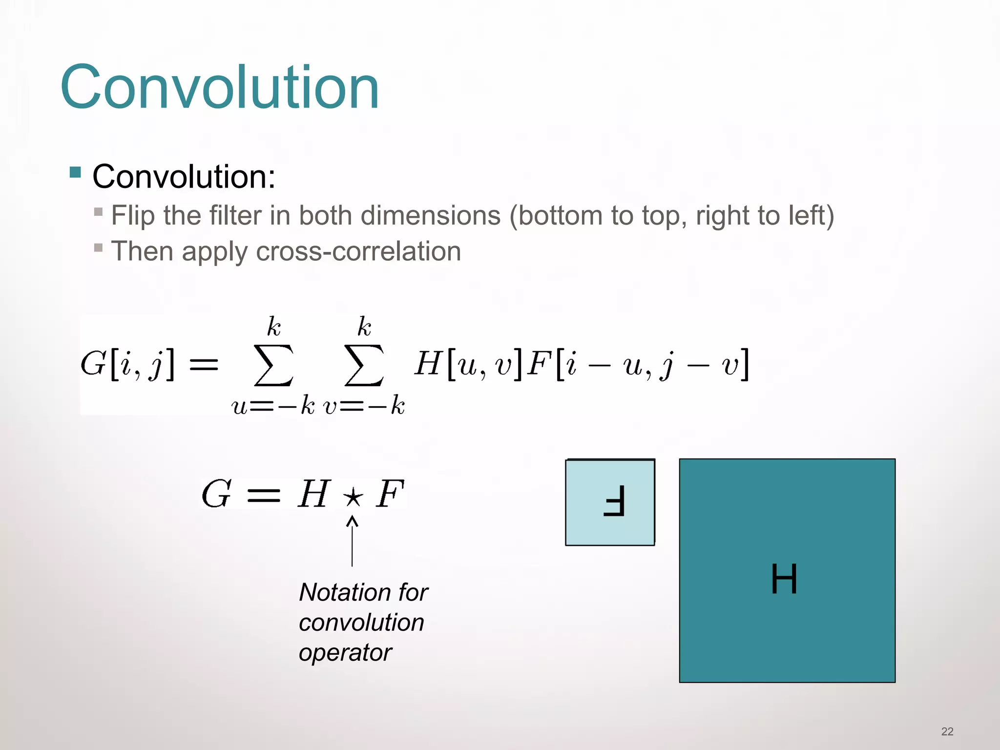
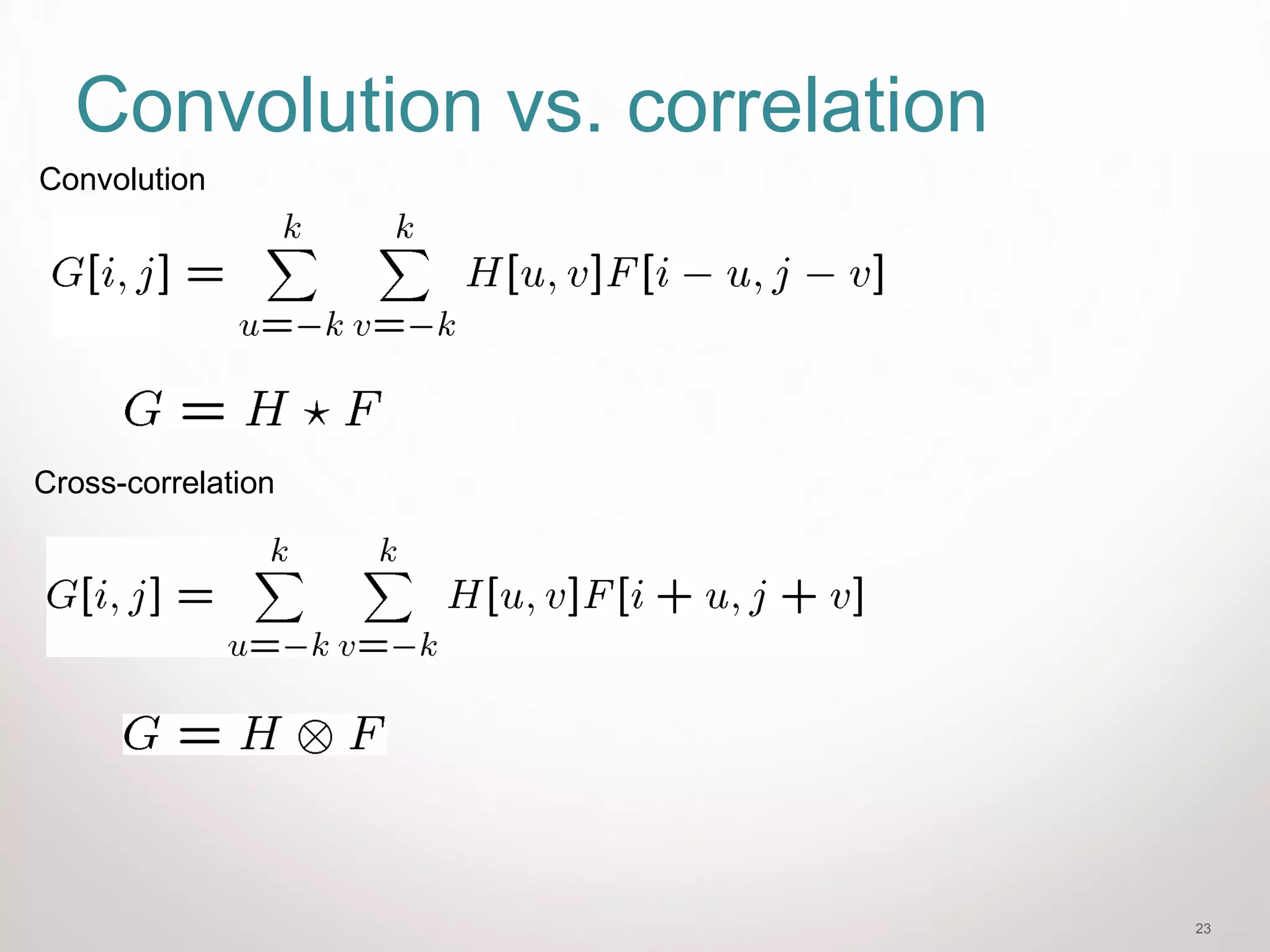
This is called cross-correlation, denoted](https://image.slidesharecdn.com/2filters-170112120805/75/Computer-Vision-Image-Filters-5-2048.jpg)
![25
More properties
• Commutative: a * b = b * a
Conceptually no difference between filter and signal
But particular filtering implementations might break this equality
• Associative: a * (b * c) = (a * b) * c
Often apply several filters one after another: (((a * b1) * b2) * b3)
This is equivalent to applying one filter: a * (b1 * b2 * b3)
• Distributes over addition: a * (b + c) = (a * b) + (a * c)
• Scalars factor out: ka * b = a * kb = k (a * b)
• Identity: unit impulse e = [0, 0, 1, 0, 0],
a * e = a Source: S. Lazebnik](https://image.slidesharecdn.com/2filters-170112120805/75/Computer-Vision-Image-Filters-25-2048.jpg)
![27
Lets try to blur filter
%%basic image filters
imrgb = imread('peppers.png');
imshow(imrgb);
a = [1 1 1; 1 1 1; 1 1 1]
Corroutimg = filter2(a, imgray);
Convoutimg = conv2(imgray,a);
figure;
imshow(Corroutimg)
figure
imshow(Convoutimg)](https://image.slidesharecdn.com/2filters-170112120805/75/Computer-Vision-Image-Filters-27-2048.jpg)
![30
Sharp
%%basic sharp filter
imrgb = imread('peppers.png');
imgray =
im2double(rgb2gray(imrgb));
imshow(imgray);
a = [ 0 0 0; 0 2 0; 0 0 0] -
1/9*ones(3)
Corroutimg = filter2(a,
imgray);
figure;
imshow(Corroutimg)](https://image.slidesharecdn.com/2filters-170112120805/75/Computer-Vision-Image-Filters-30-2048.jpg)


![3
How to filter
2d Correlation
h=filter2(g,f); or h=imfilter(f,g);
2d Convolution
h=conv2(g,f);
],[],[],[
,
lnkmflkgnmh
lk
−−= ∑
f=image
g=filter
],[],[],[
,
lnkmflkgnmh
lk
++= ∑](https://crownmelresort.com/image.slidesharecdn.com/2filters-170112120805/75/Computer-Vision-Image-Filters-3-2048.jpg)
![4
Correlation filtering
Say the averaging window size is 2k+1 x 2k+1:
Loop over all pixels in neighborhood around
image pixel F[i,j]
Attribute uniform
weight to each pixel
Now generalize to allow different weights depending on
neighboring pixel’s relative position:
Non-uniform weights](https://crownmelresort.com/image.slidesharecdn.com/2filters-170112120805/75/Computer-Vision-Image-Filters-4-2048.jpg)
![5
Correlation filtering
Filtering an image: replace each pixel with a linear
combination of its neighbors.
The filter “kernel” or “mask” H[u,v] is the prescription for the
weights in the linear combination.
This is called cross-correlation, denoted](https://crownmelresort.com/image.slidesharecdn.com/2filters-170112120805/75/Computer-Vision-Image-Filters-5-2048.jpg)


![25
More properties
• Commutative: a * b = b * a
Conceptually no difference between filter and signal
But particular filtering implementations might break this equality
• Associative: a * (b * c) = (a * b) * c
Often apply several filters one after another: (((a * b1) * b2) * b3)
This is equivalent to applying one filter: a * (b1 * b2 * b3)
• Distributes over addition: a * (b + c) = (a * b) + (a * c)
• Scalars factor out: ka * b = a * kb = k (a * b)
• Identity: unit impulse e = [0, 0, 1, 0, 0],
a * e = a Source: S. Lazebnik](https://crownmelresort.com/image.slidesharecdn.com/2filters-170112120805/75/Computer-Vision-Image-Filters-25-2048.jpg)

![27
Lets try to blur filter
%%basic image filters
imrgb = imread('peppers.png');
imshow(imrgb);
a = [1 1 1; 1 1 1; 1 1 1]
Corroutimg = filter2(a, imgray);
Convoutimg = conv2(imgray,a);
figure;
imshow(Corroutimg)
figure
imshow(Convoutimg)](https://crownmelresort.com/image.slidesharecdn.com/2filters-170112120805/75/Computer-Vision-Image-Filters-27-2048.jpg)


![30
Sharp
%%basic sharp filter
imrgb = imread('peppers.png');
imgray =
im2double(rgb2gray(imrgb));
imshow(imgray);
a = [ 0 0 0; 0 2 0; 0 0 0] -
1/9*ones(3)
Corroutimg = filter2(a,
imgray);
figure;
imshow(Corroutimg)](https://crownmelresort.com/image.slidesharecdn.com/2filters-170112120805/75/Computer-Vision-Image-Filters-30-2048.jpg)


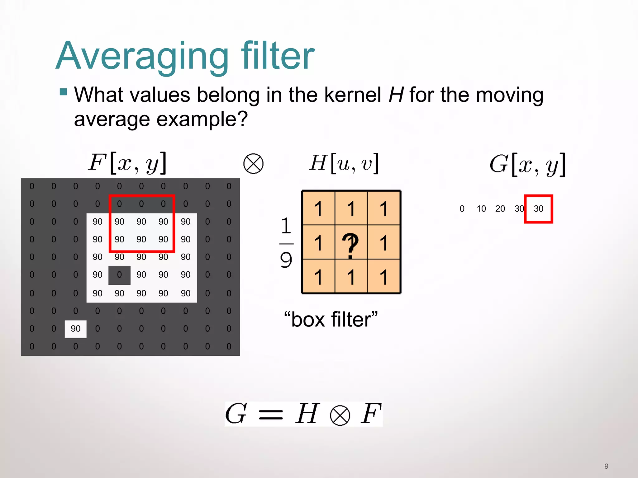
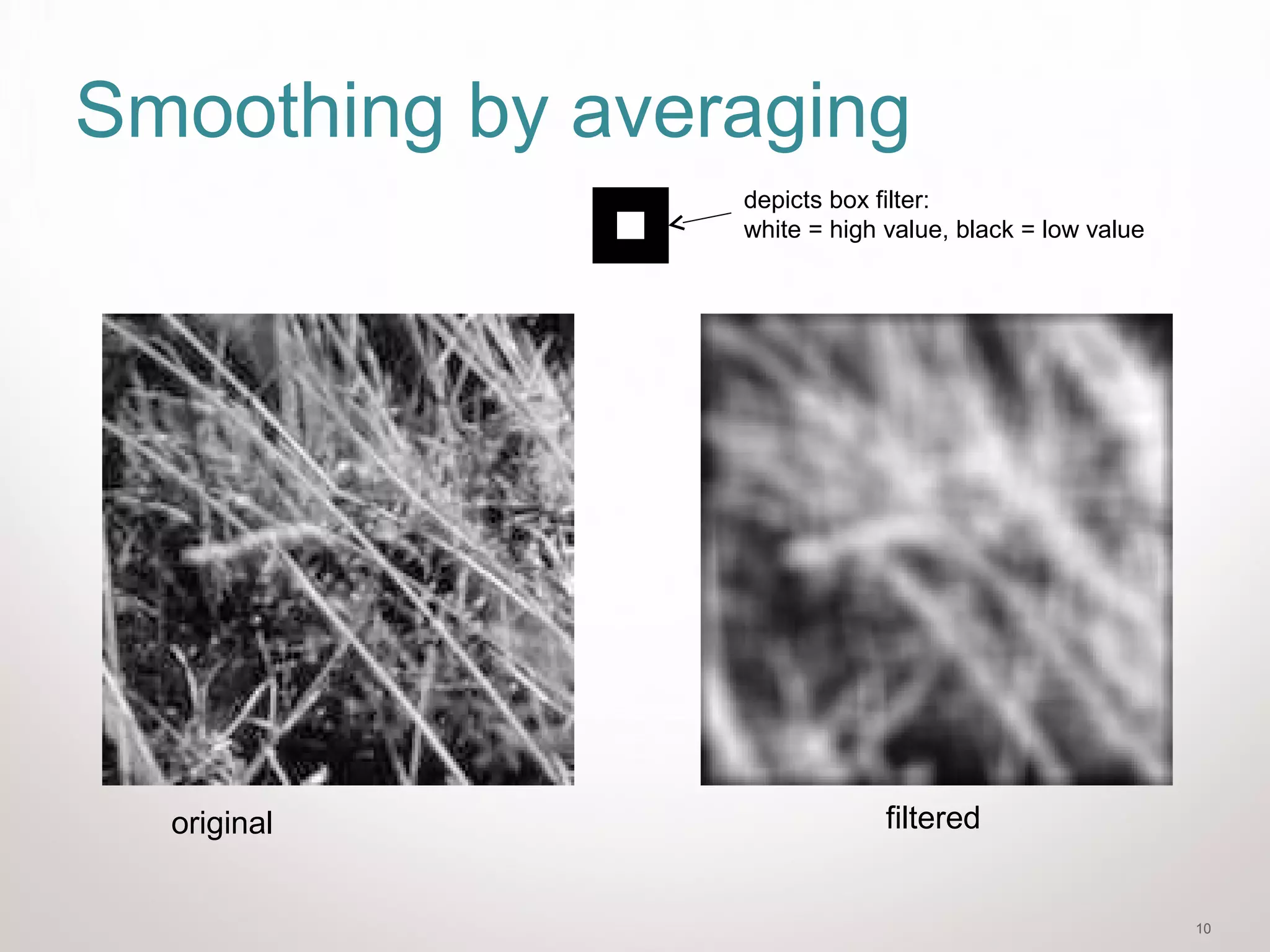
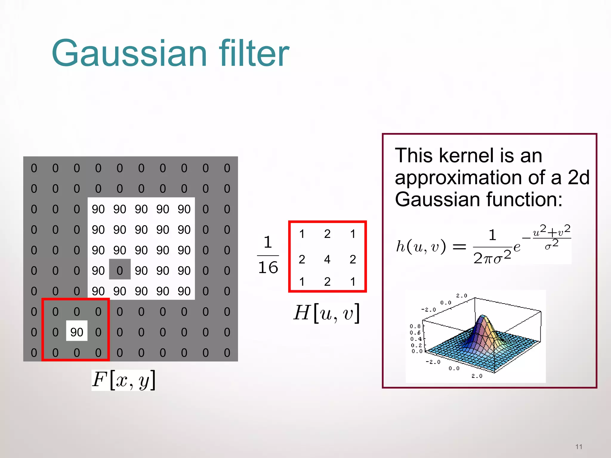
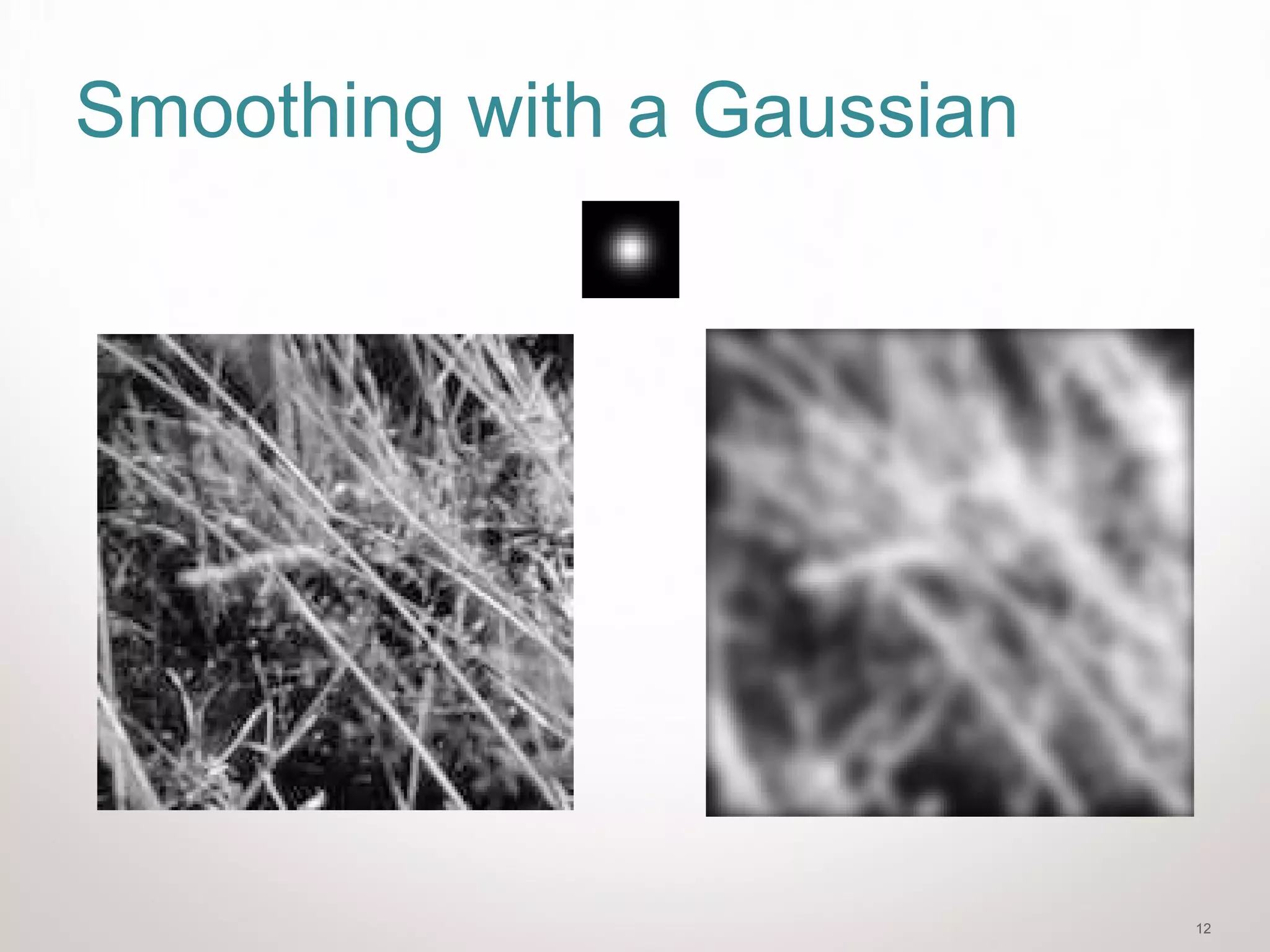
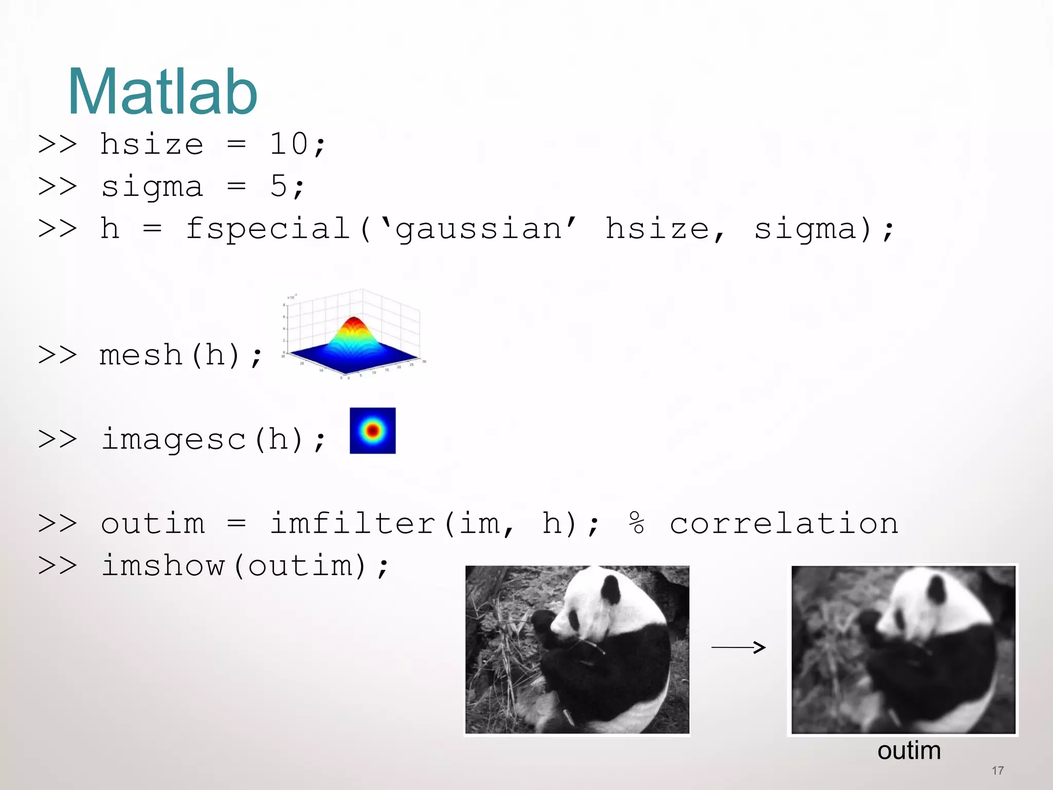
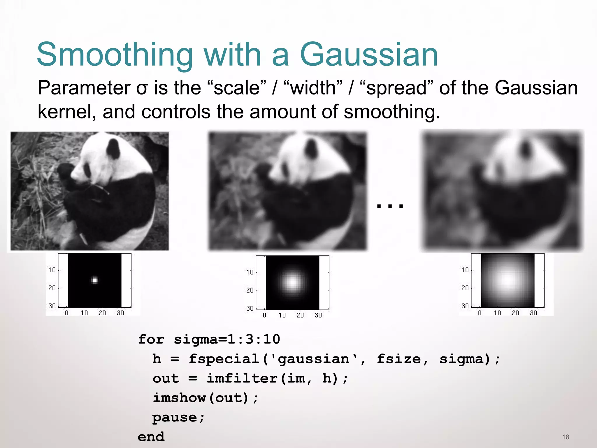
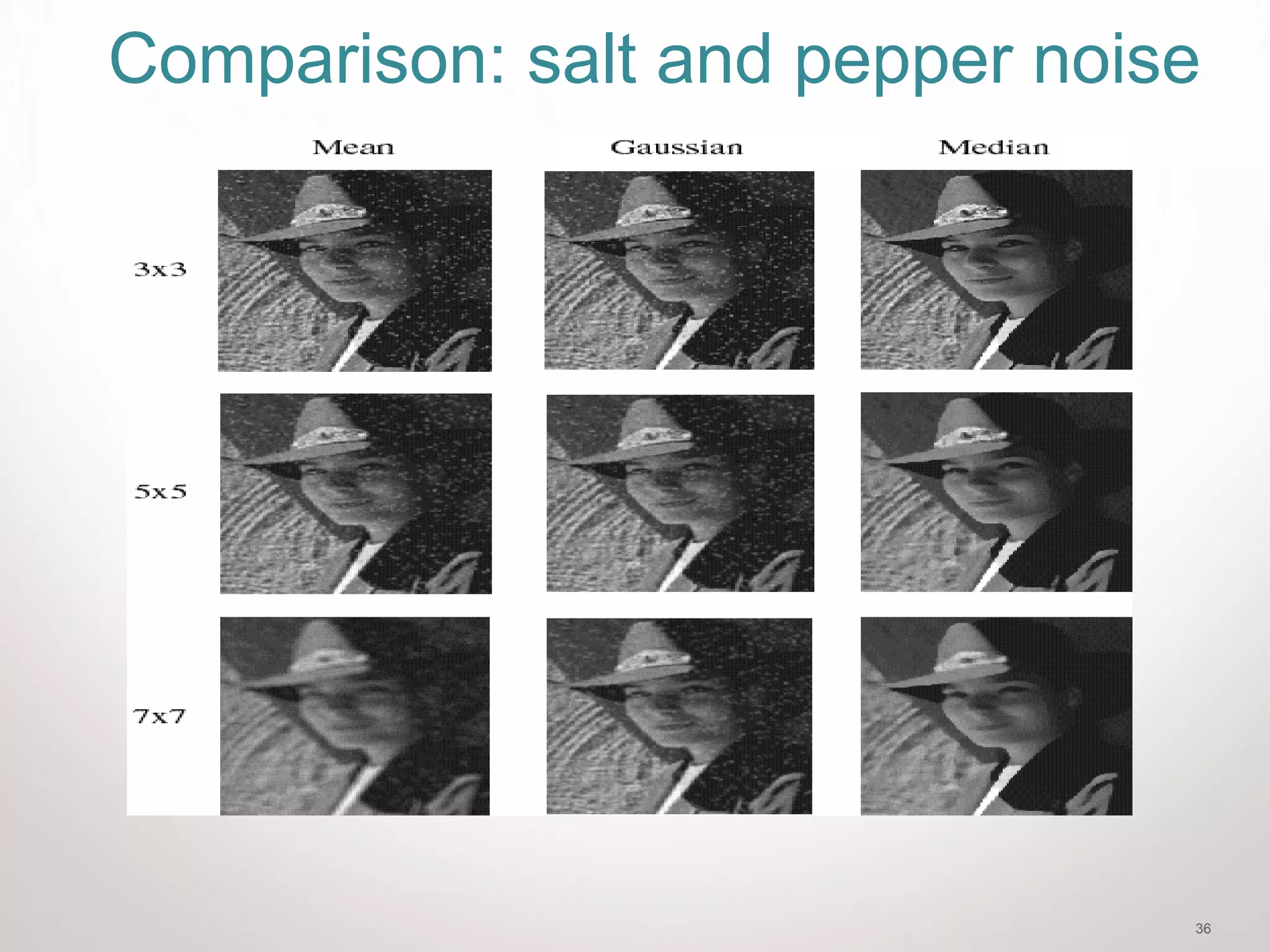
1. The document discusses various image filtering techniques, including correlation filtering, convolution, averaging filters, and Gaussian filters. 2. Gaussian filters are commonly used for smoothing images as they remove high-frequency components while maintaining edges. The scale parameter σ controls the amount of smoothing. 3. Median filters can reduce noise in images by selecting the median value in a local neighborhood, unlike mean filters which are susceptible to outliers.
Introduction to the domain of computer vision, setting the context for subsequent discussions.
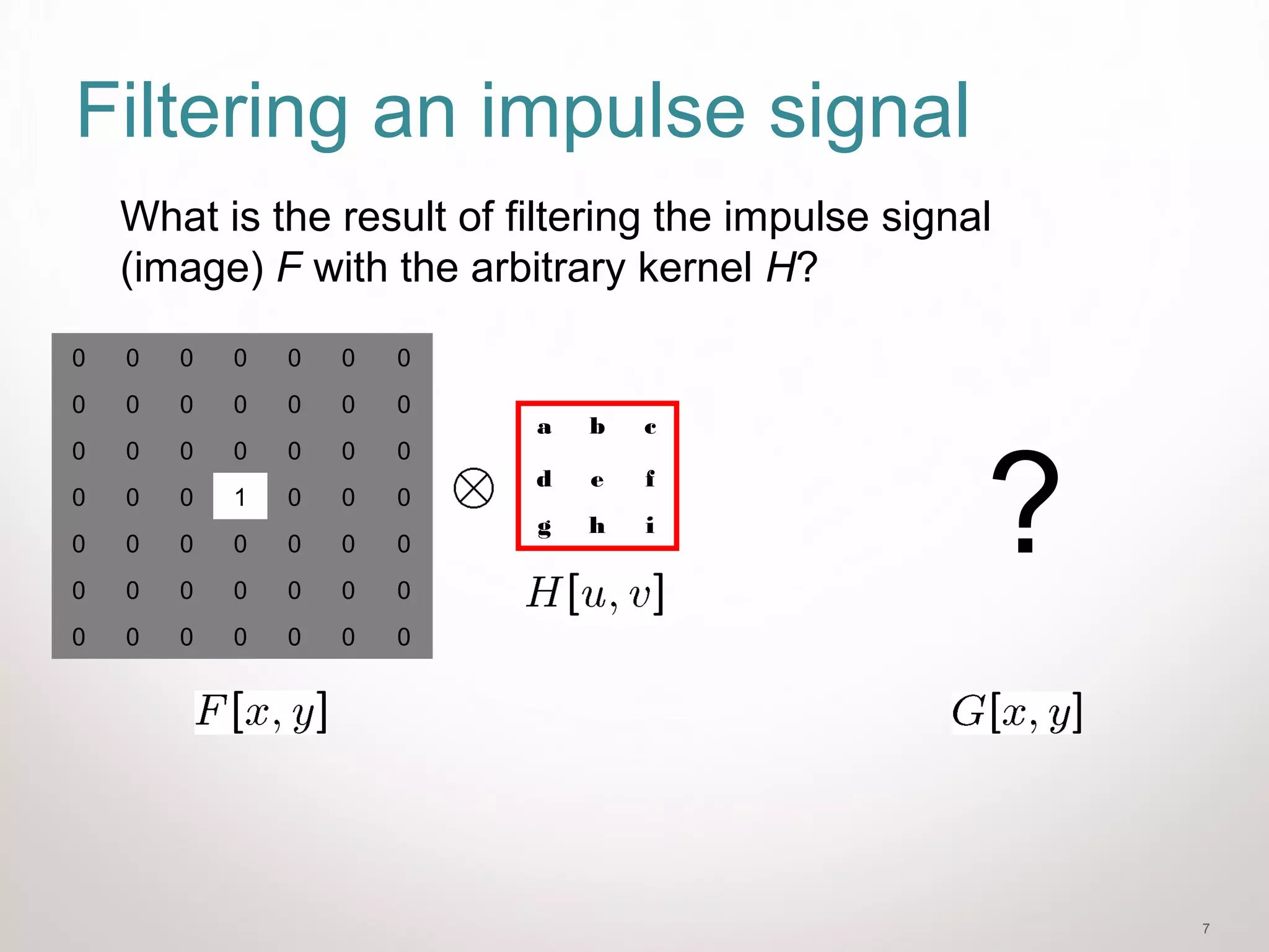
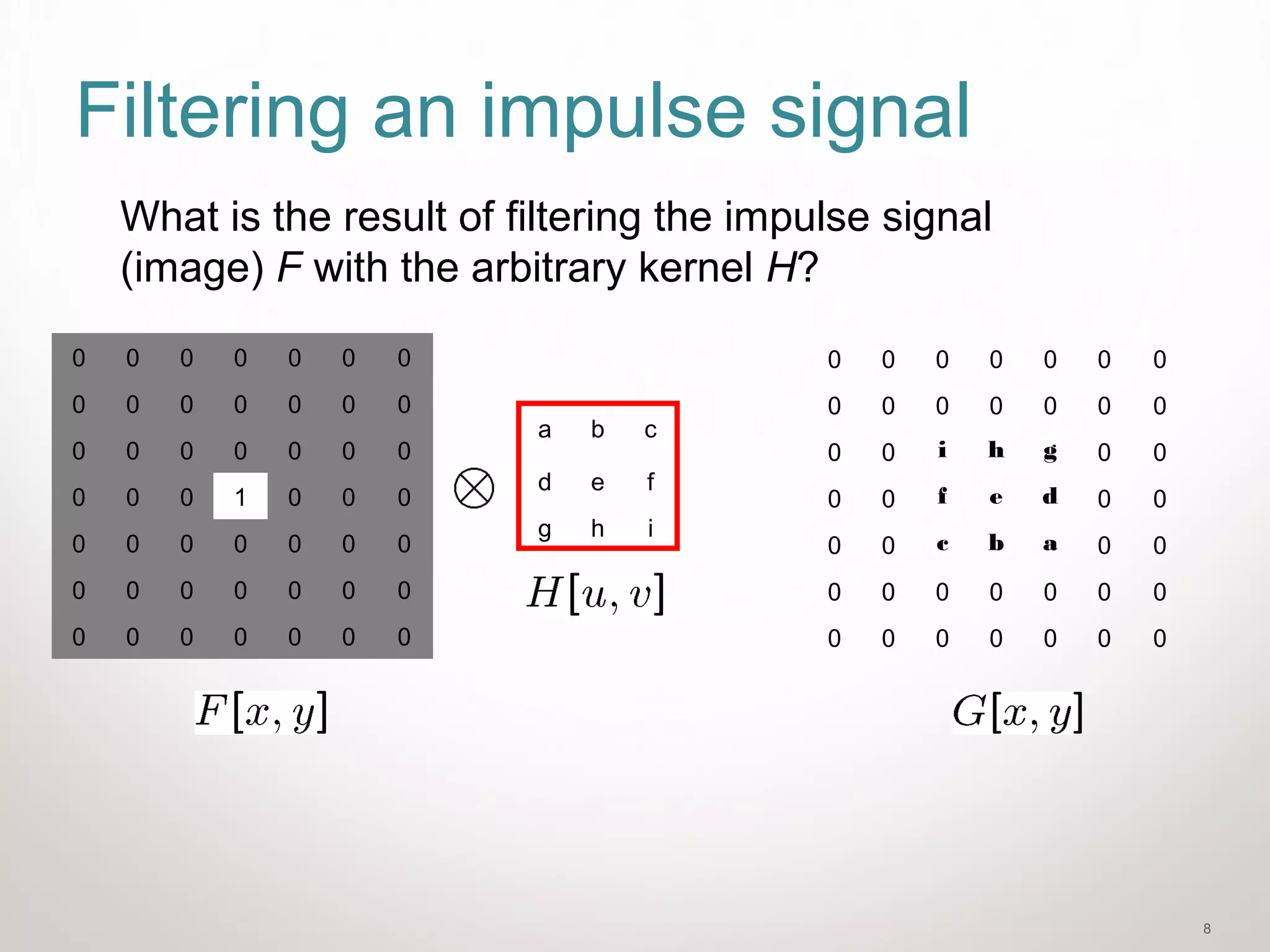
Overview of filtering in image processing, including 2D correlation, convolution, and averaging filters.
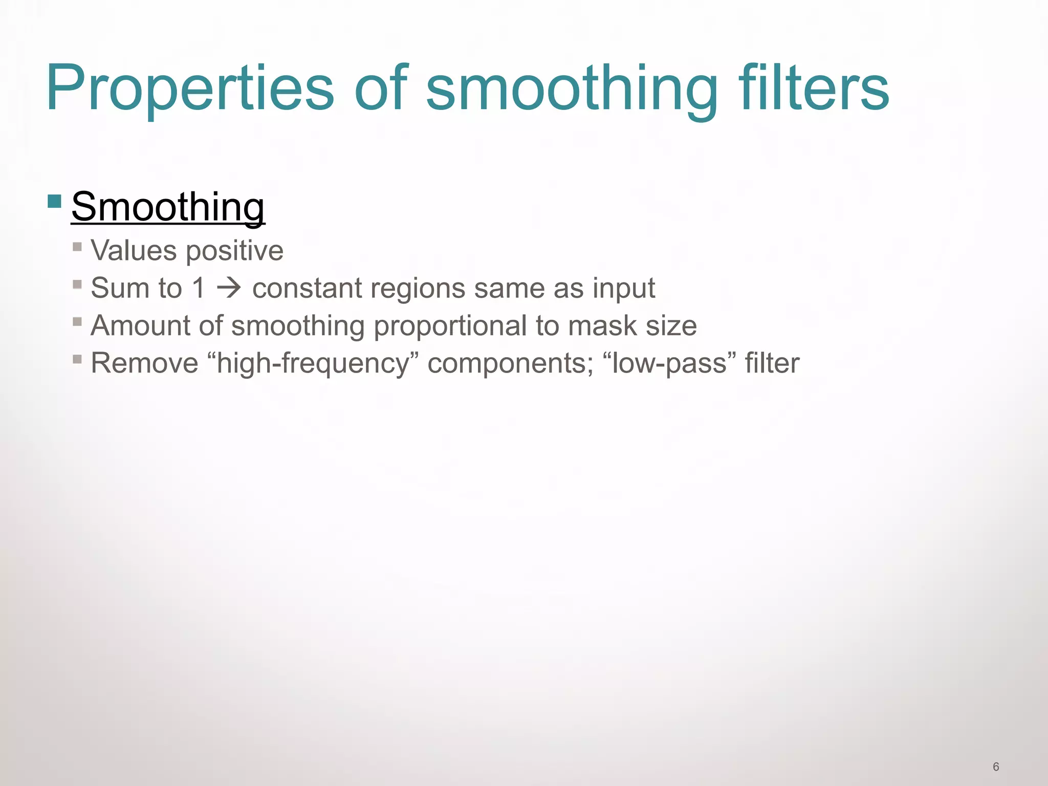
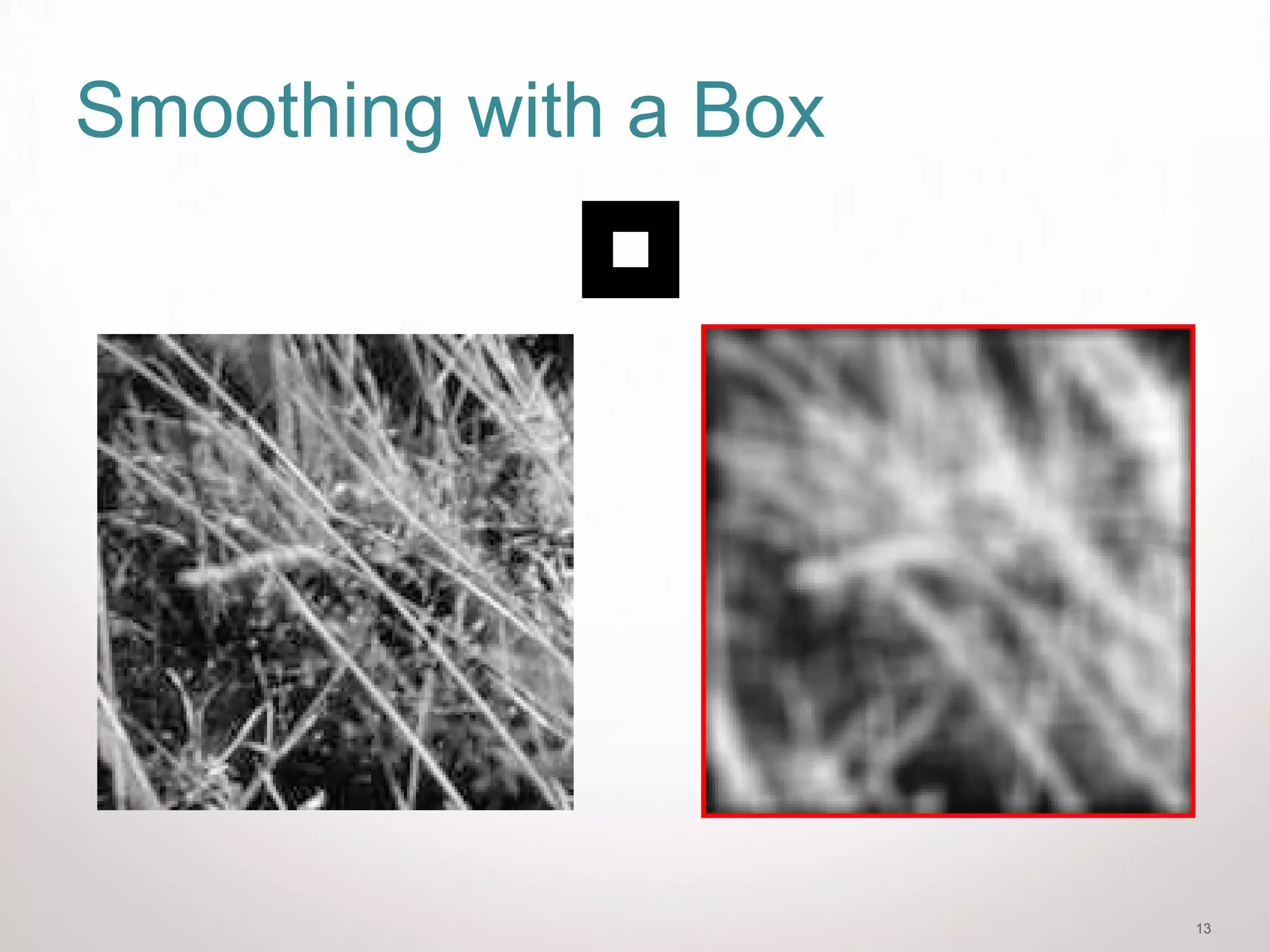
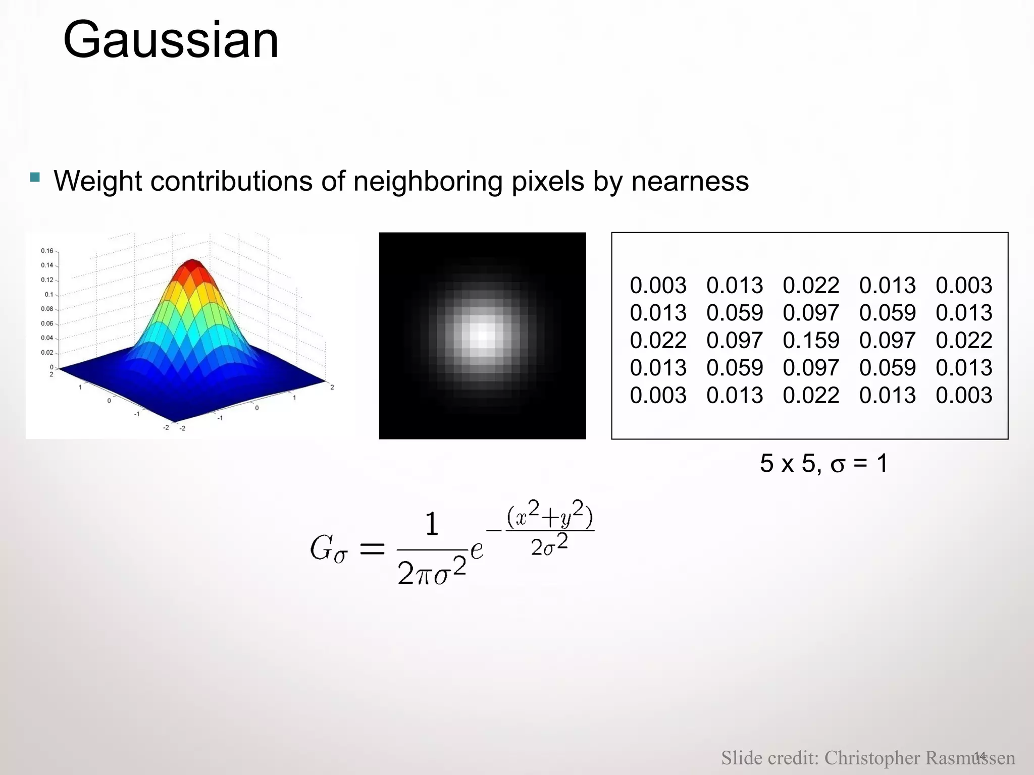
Discussion of averaging and Gaussian filters for smoothing images and reducing noise.
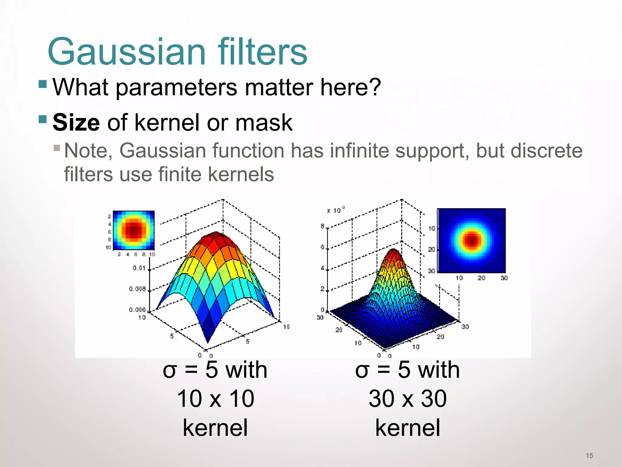
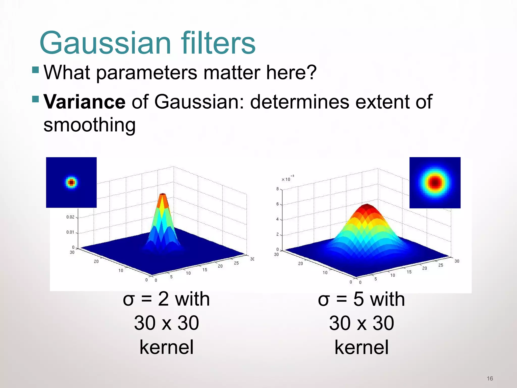
Examination of Gaussian filter parameters, their effects on smoothing, and kernel sizes.
MATLAB code examples for creating and applying Gaussian filters, illustrating practical usage.
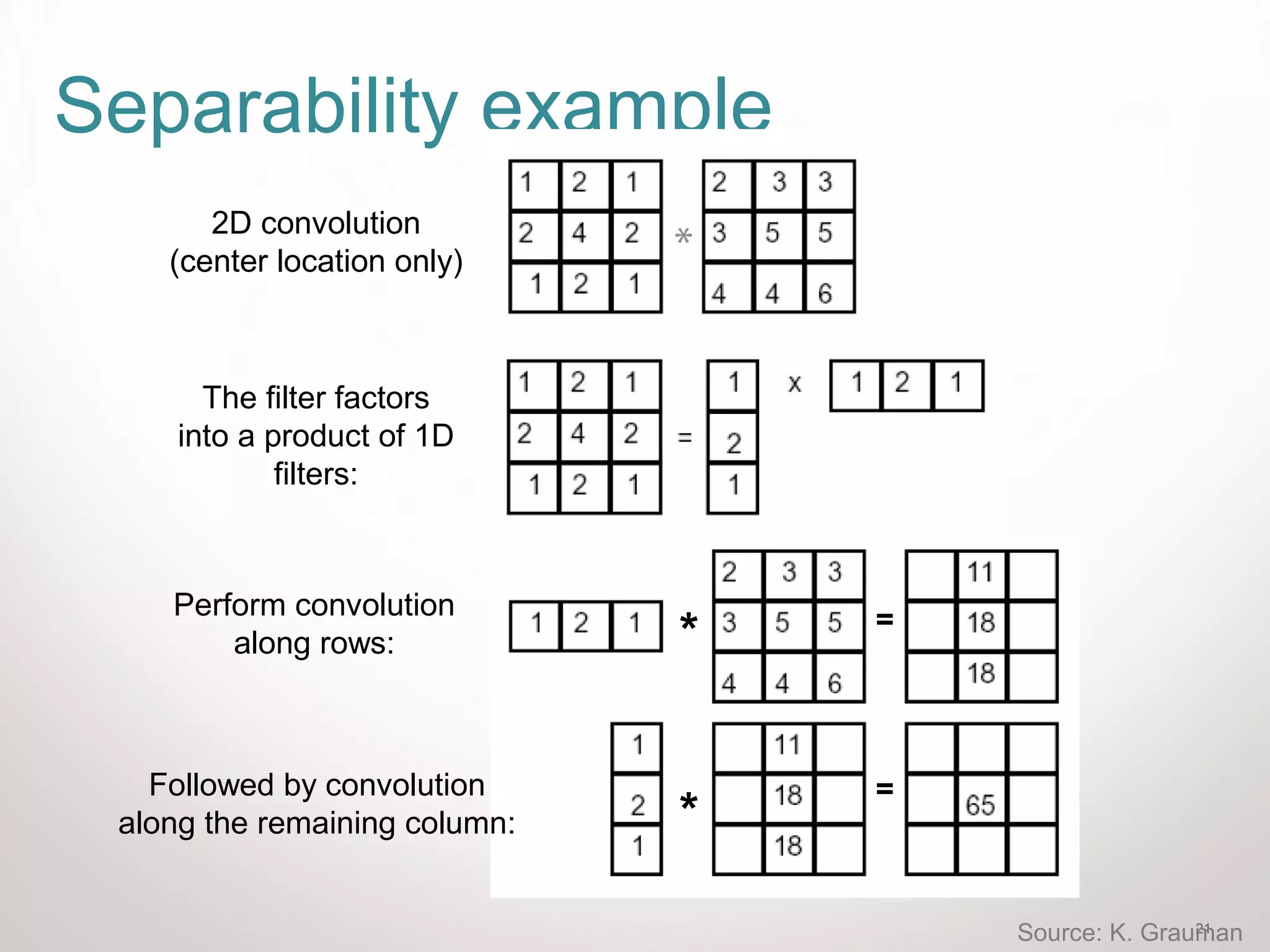
Characteristics of Gaussian filters, including separability and convolution definitions.
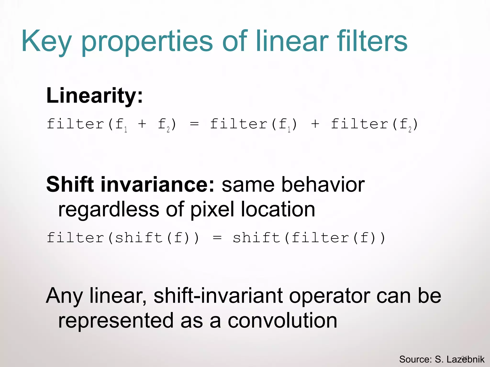
Fundamental properties of linear filters, such as linearity and shift invariance.
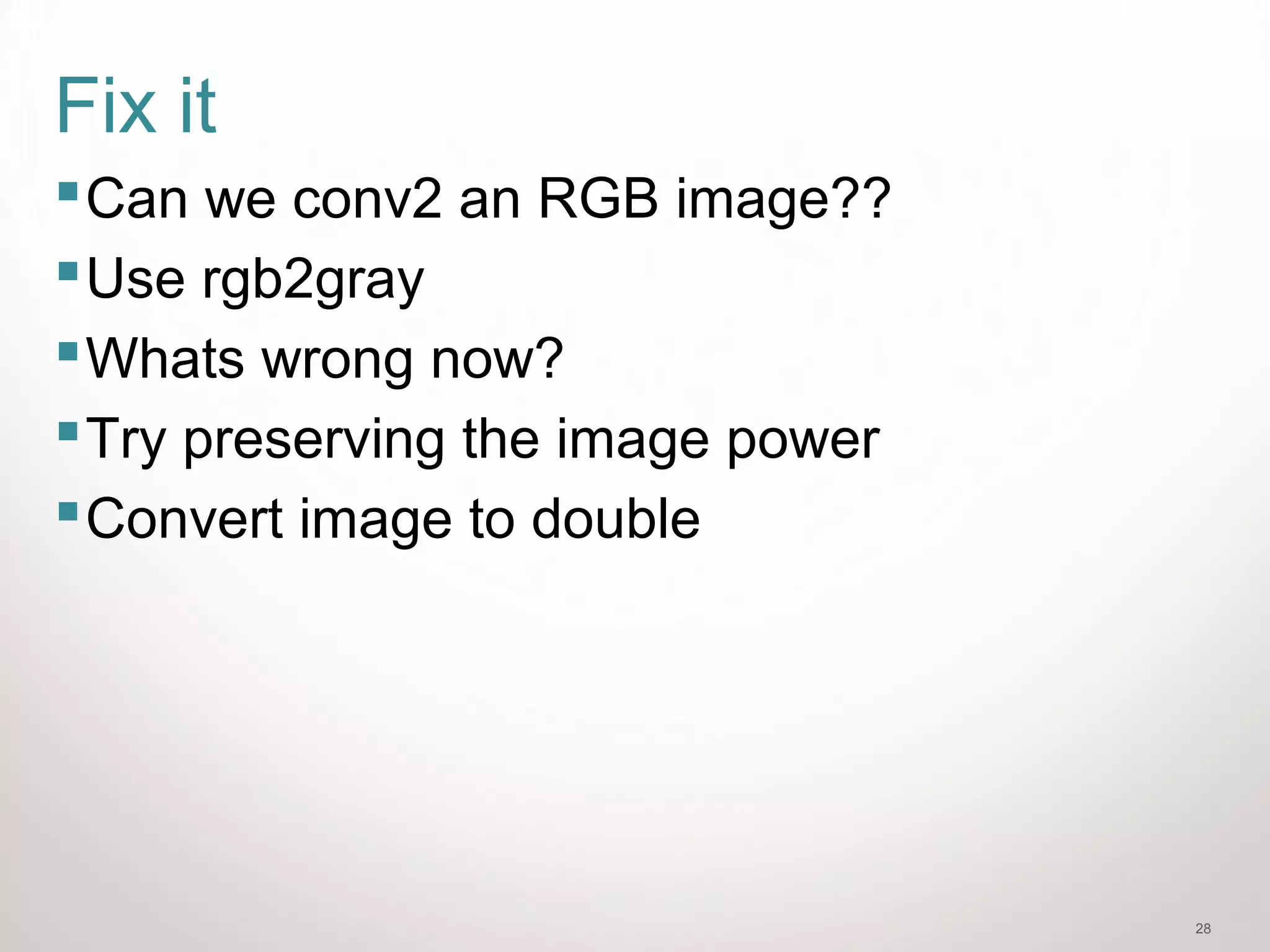
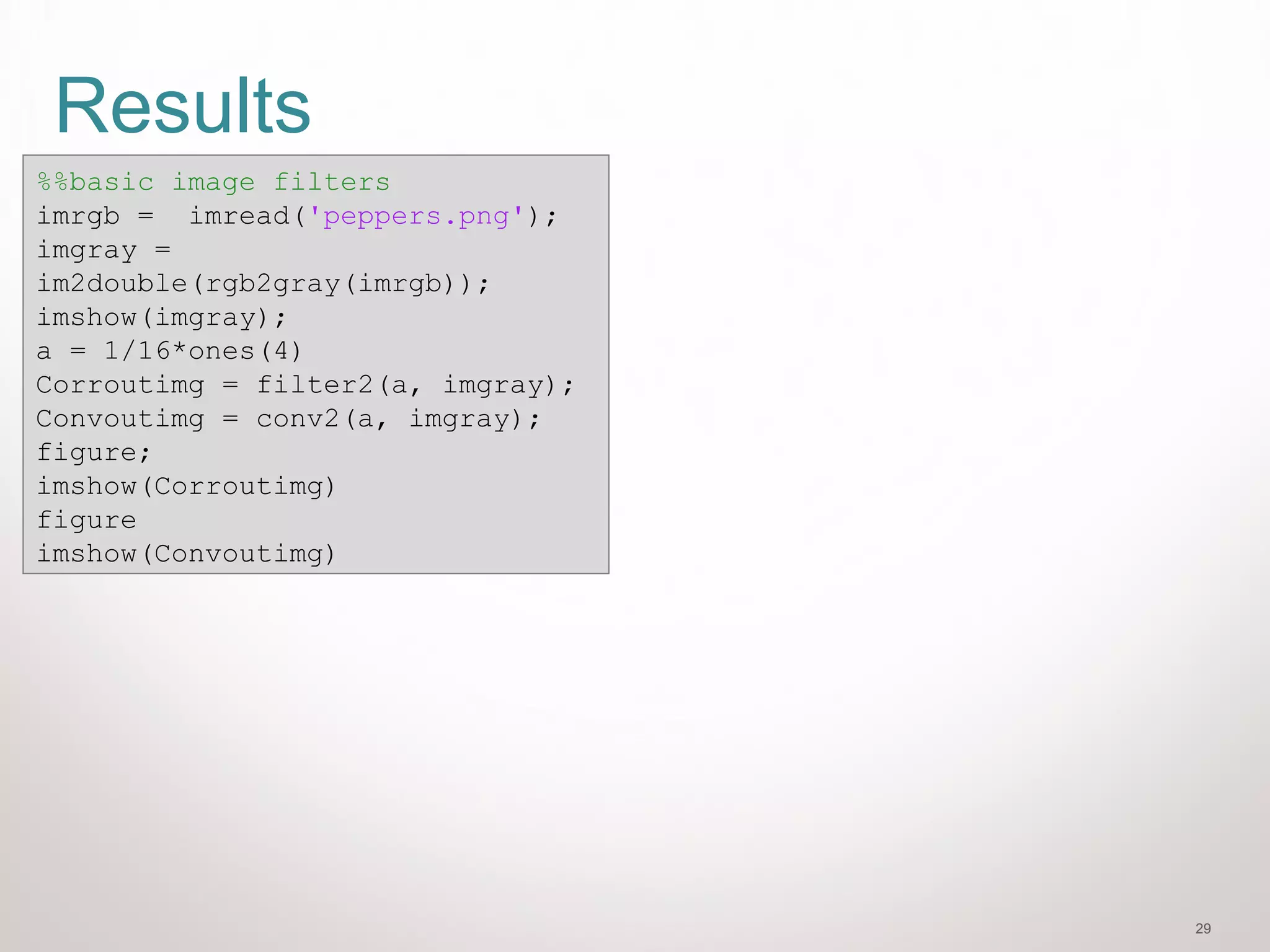
Practical application of basic image filters in MATLAB, focusing on RGB to grayscale conversions.
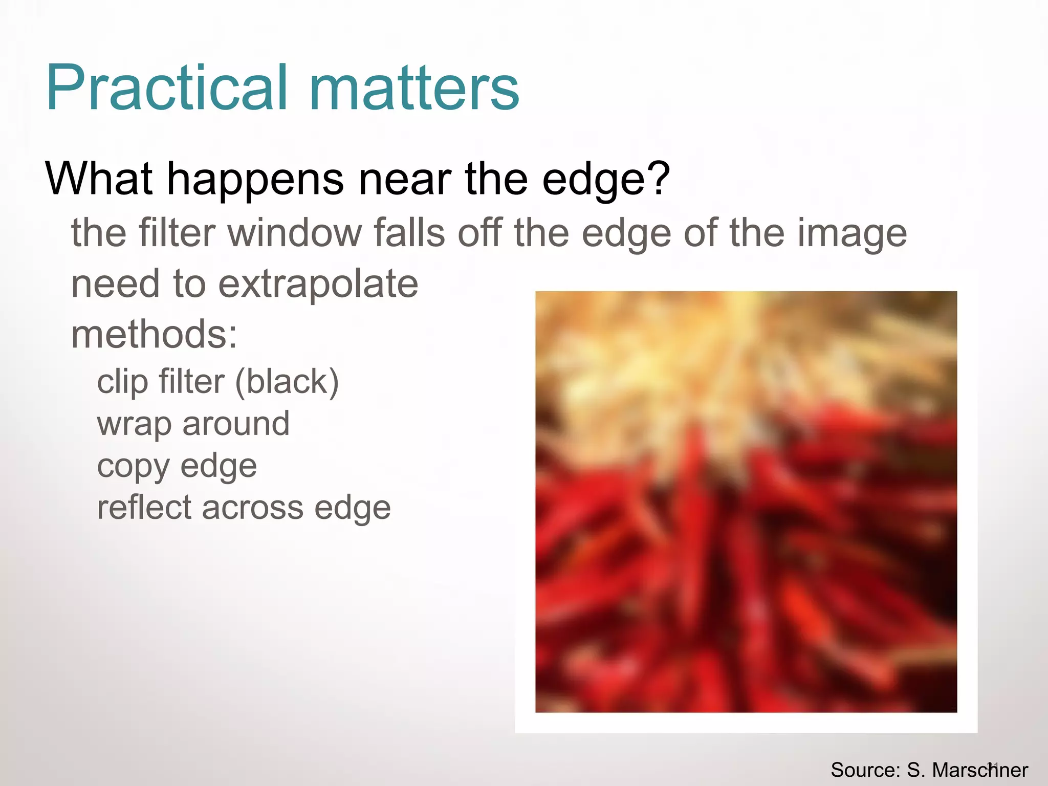
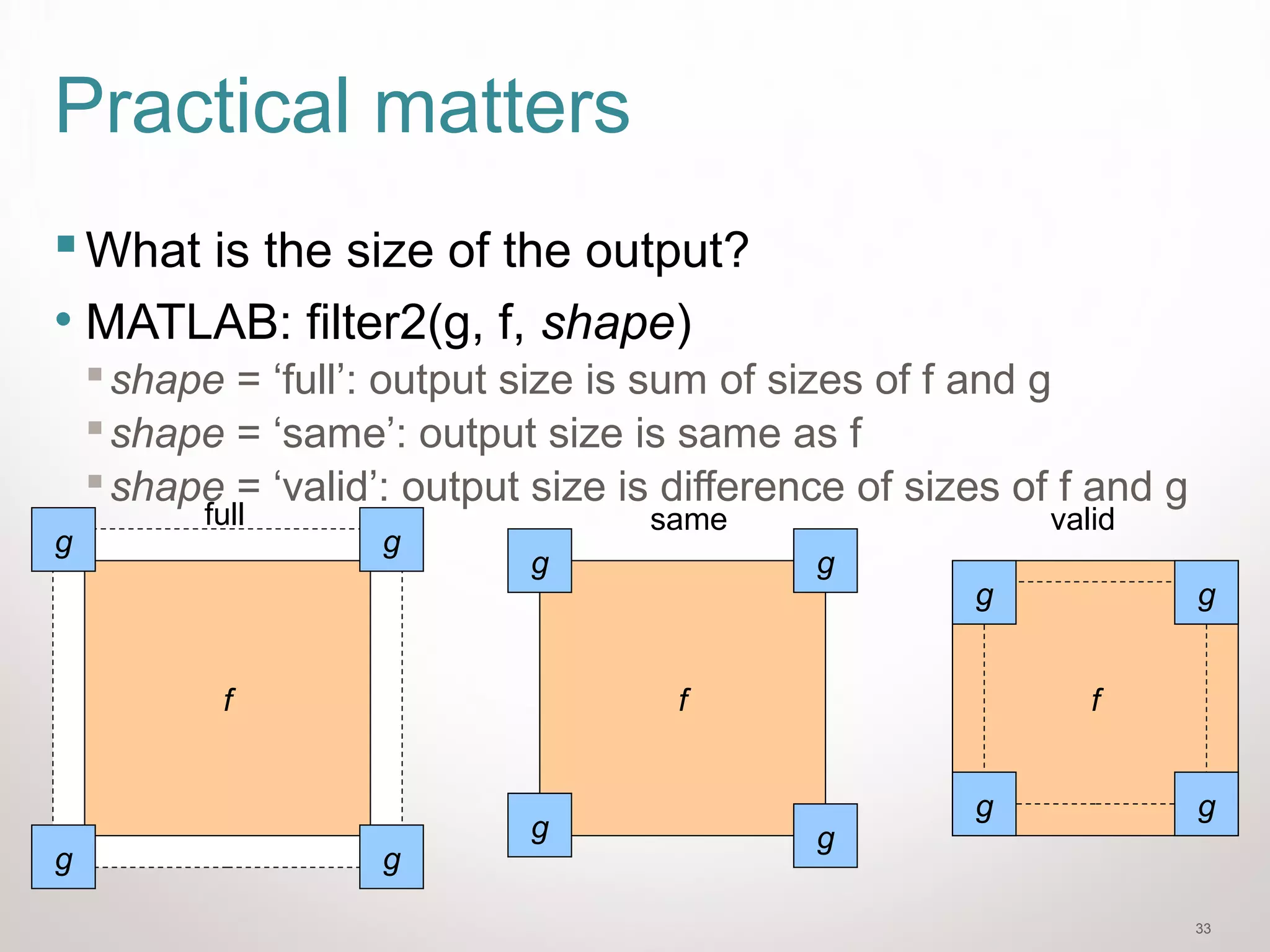
Discussion on handling image edges during filtering and methods available in MATLAB.
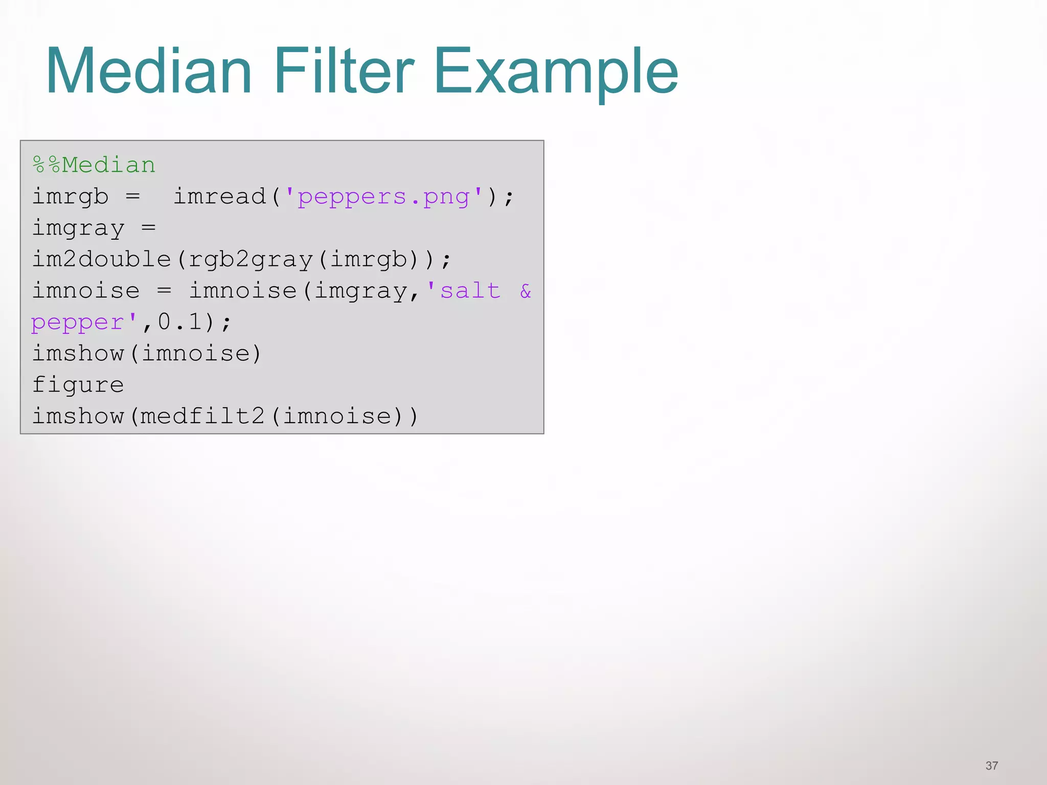
Description of median filters, their advantages over mean filters, and comparison with salt and pepper noise.