This document provides an overview of image processing using MATLAB. It discusses how images are represented as matrices in MATLAB and demonstrates various image processing functions and techniques.
Key points covered include:
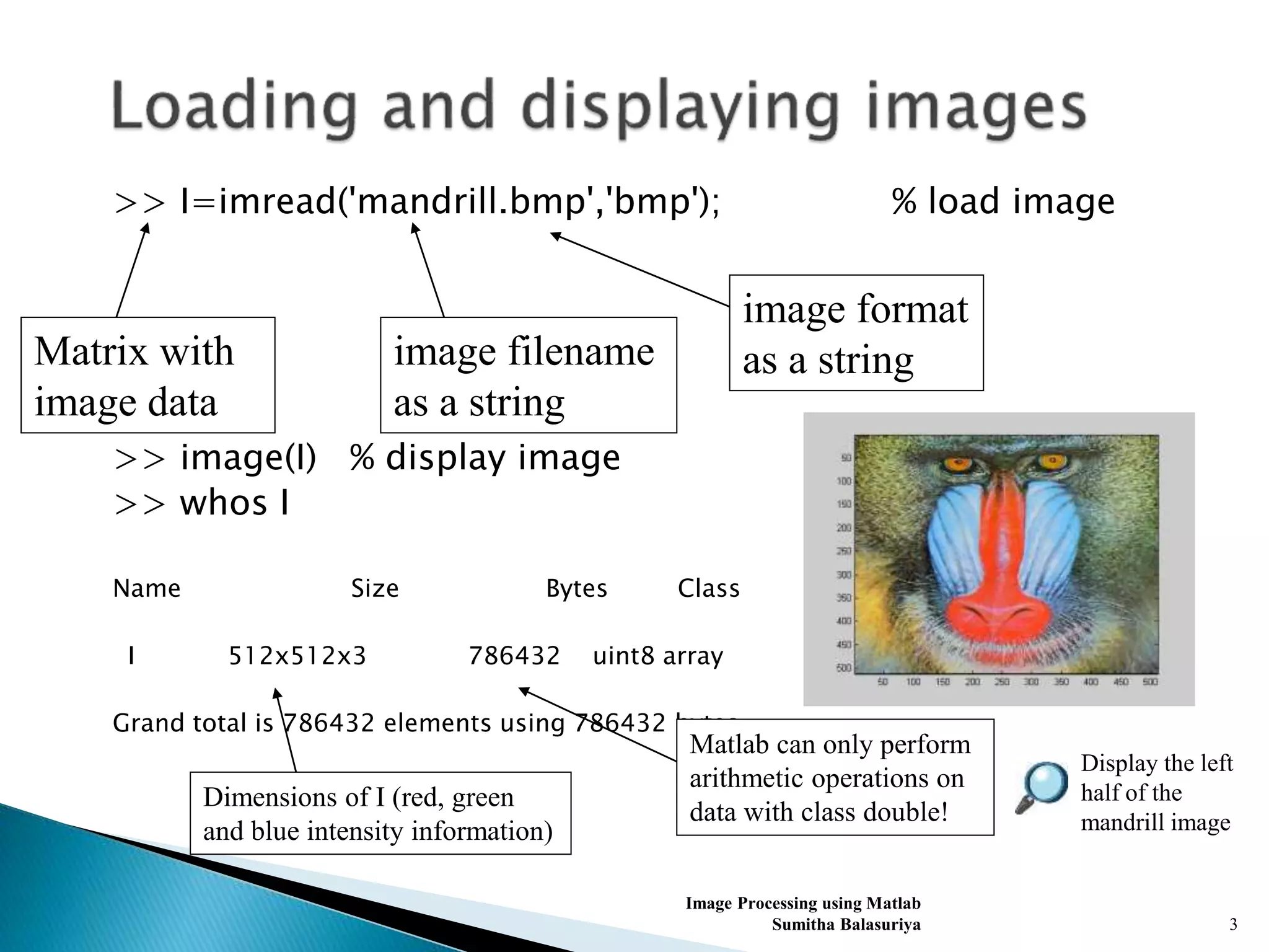
- Loading and displaying an image using imread and image commands
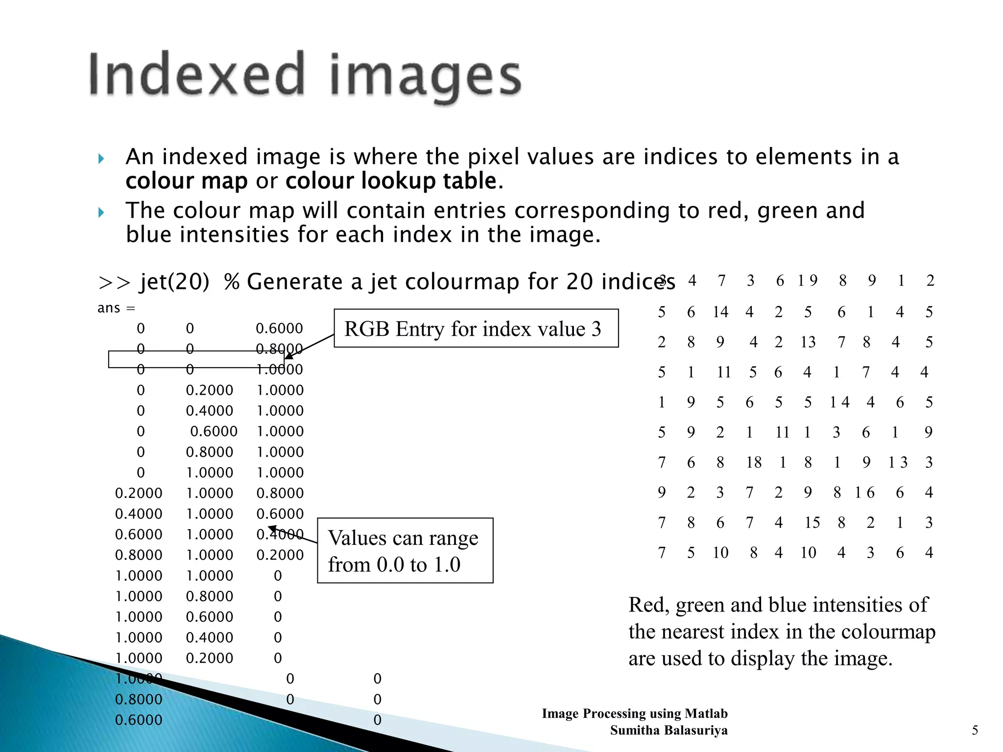
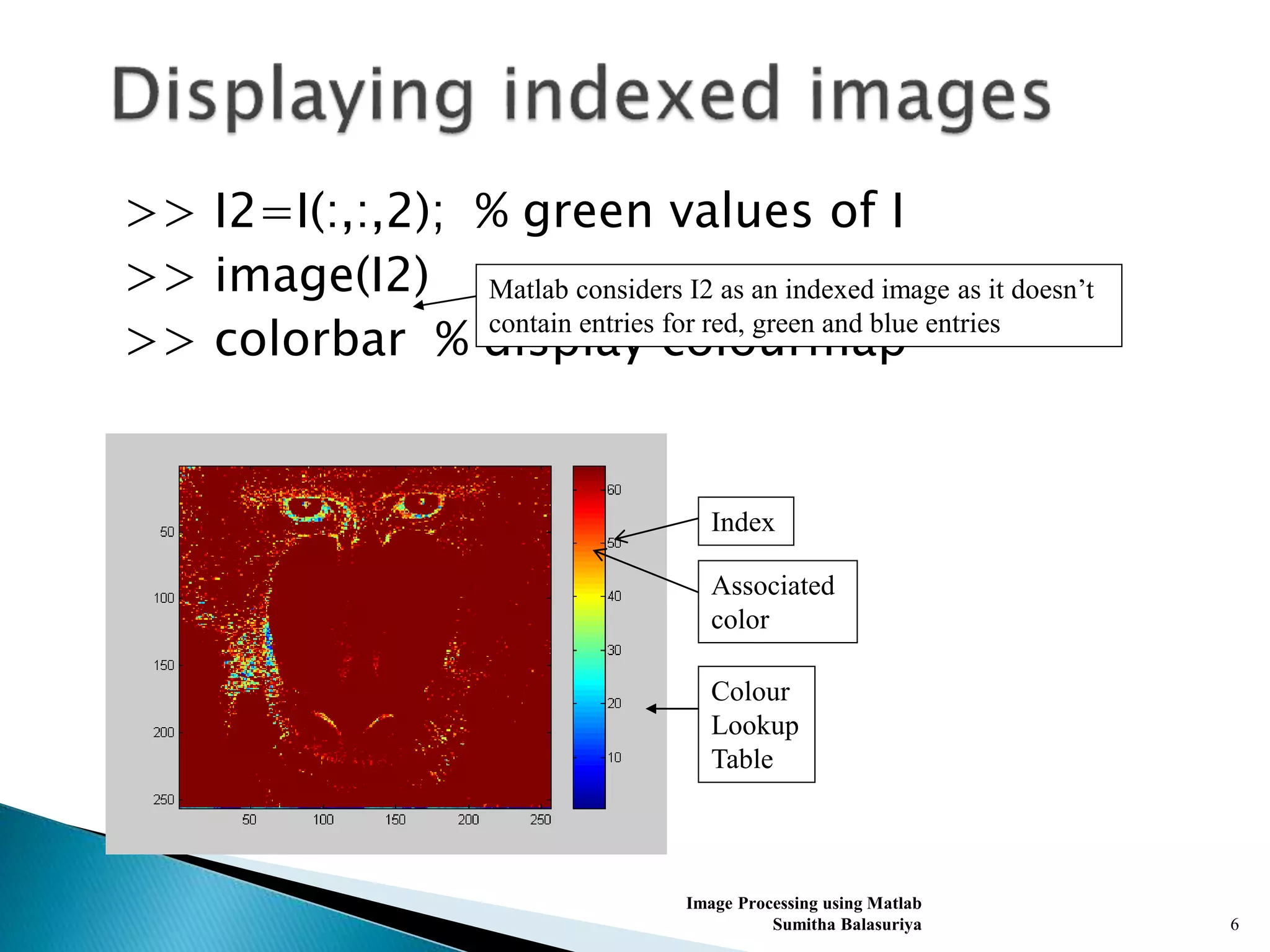
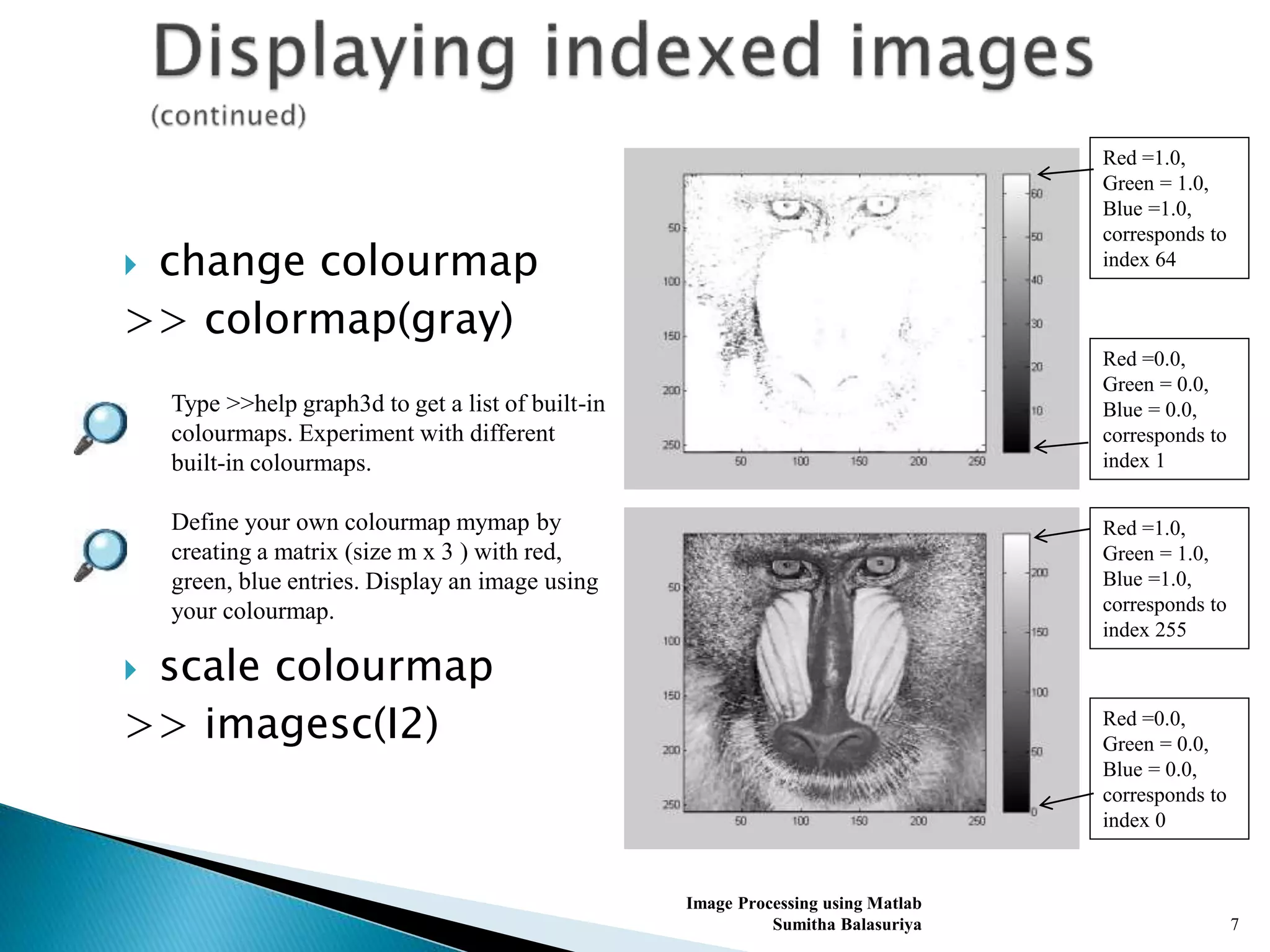
- Converting between intensity, indexed, and RGB image representations
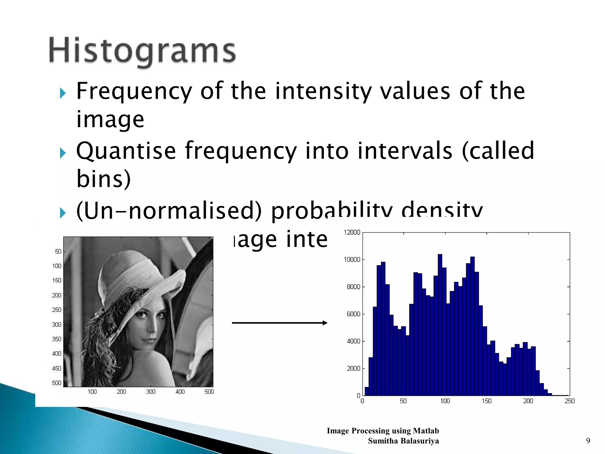
- Exploring image histograms and equalization
- Performing operations like resizing, rotation and filtering using functions like imresize, imrotate, and filters from fspecial
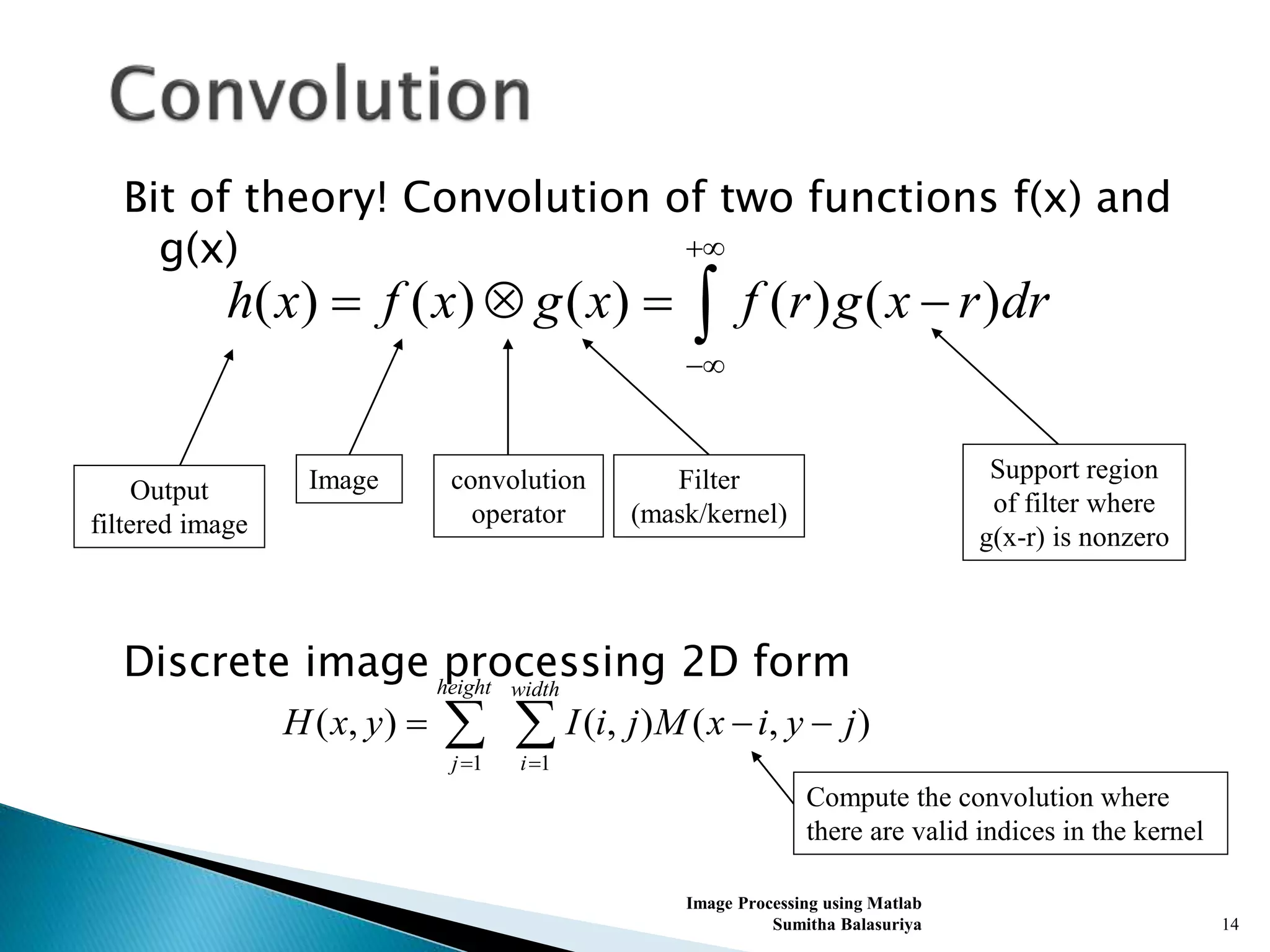
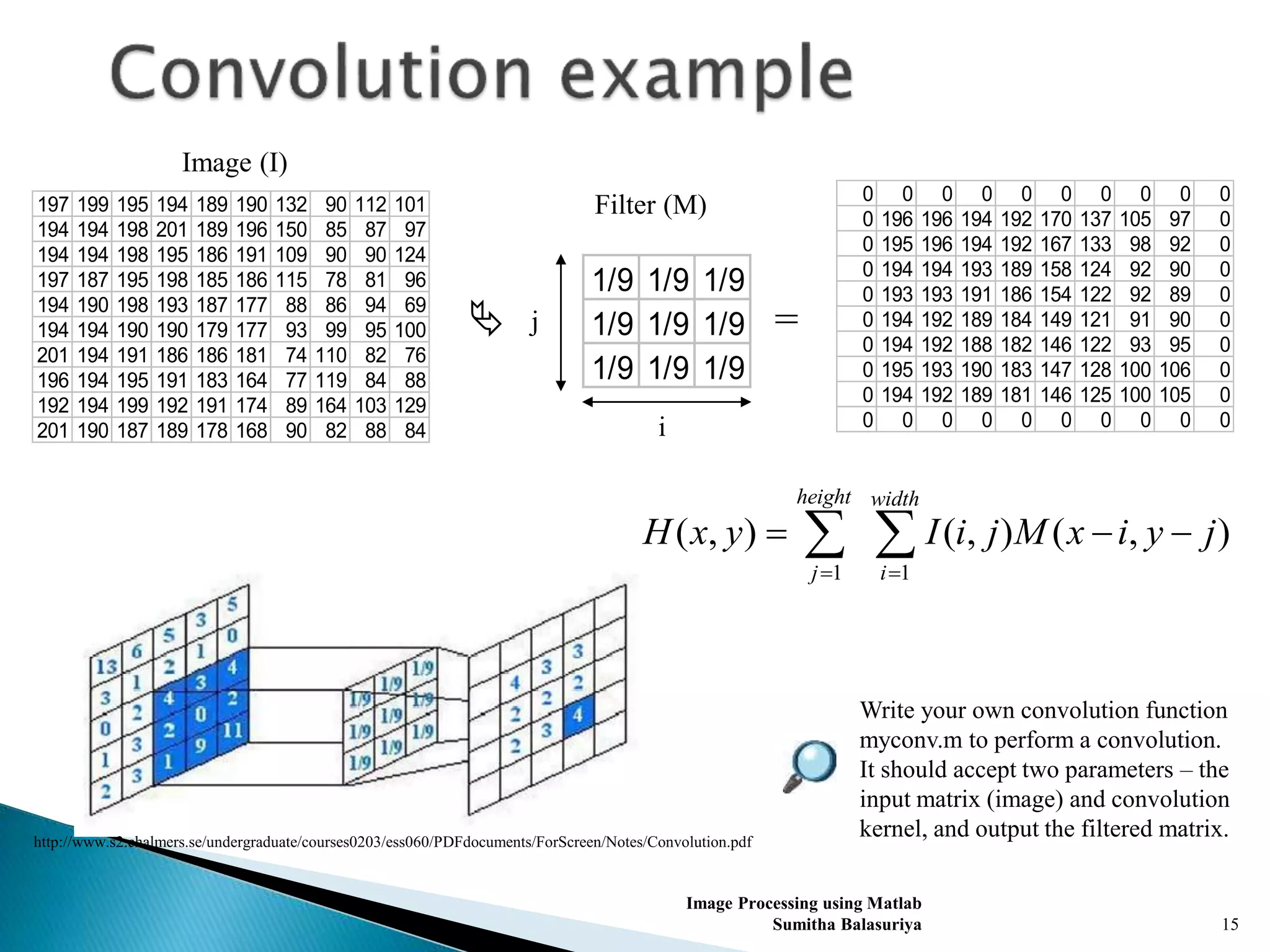
- Implementing convolution using custom kernels and built-in filters
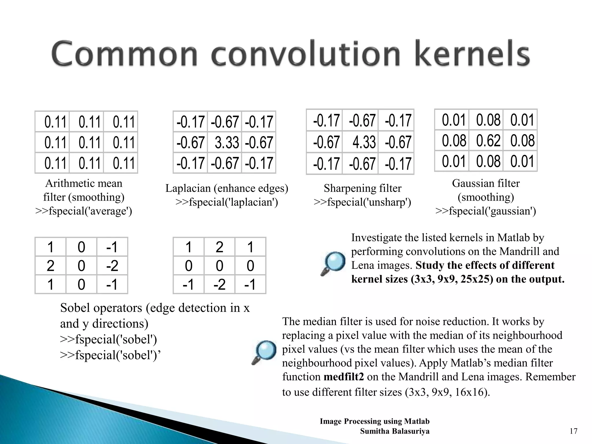
- Understanding effects of different kernels on images
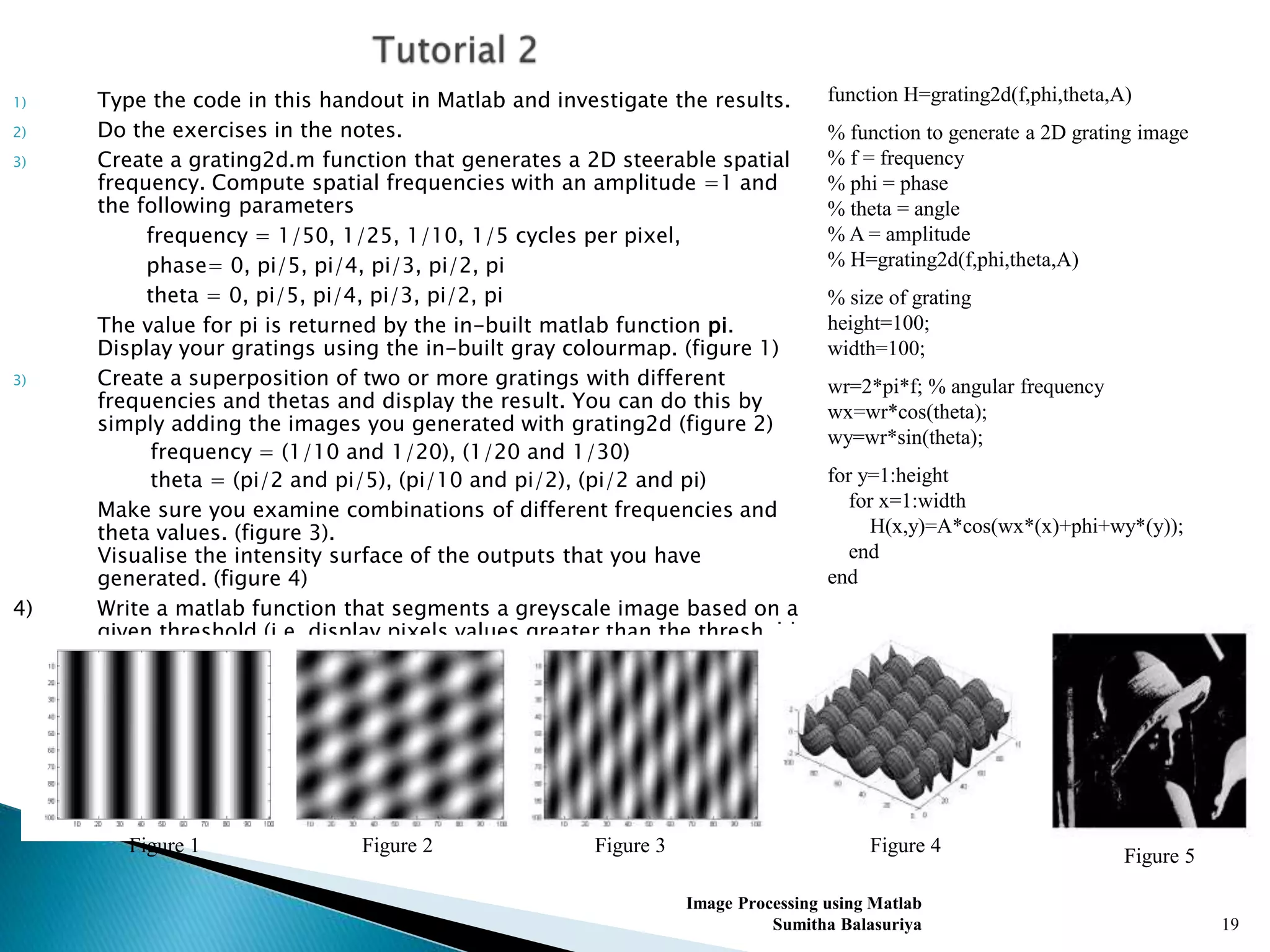
![>> axis image % plot fits to data
>> h=axes('position', [0 0 0.5 0.5]);
>> axes(h);
>> imagesc(I2)
Image Processing using Matlab
Sumitha Balasuriya 8
Investigate axis and axes
functions using Matlab’s help](https://image.slidesharecdn.com/imageprocessingusingmatlab-191220055348/75/Image-processing-using-matlab-8-2048.jpg)
![>>hist(reshape(double(Lena(:,:,2)),[512*512
1]),50)
Image Processing using Matlab
Sumitha Balasuriya 10
Convert image into a 262144 by
1 distribution of values
Histogram
function
Number of bins
Histogram equalisation works by equitably distributing the pixels among the
histogram bins. Histogram equalise the green channel of the Lena image
using Matlab’s histeq function. Compare the equalised image with the
original. Display the histogram of the equalised image. The number of pixels
in each bin should be approximately equal.
Generate the histograms of the green channel of the Lena image using the
following number of bins : 10, 20, 50, 100, 200, 500, 1000](https://image.slidesharecdn.com/imageprocessingusingmatlab-191220055348/75/Image-processing-using-matlab-10-2048.jpg)
![>>surf(double(imresize(Lena(:,:,2),[50 50])))
Image Processing using Matlab
Sumitha Balasuriya 11
Remember to reduce
size of image!
Use Matlab’s built-in mesh and
shading surface visualisation
functions
Change type to
double precision](https://image.slidesharecdn.com/imageprocessingusingmatlab-191220055348/75/Image-processing-using-matlab-11-2048.jpg)
![ Convert image to grayscale
>>Igray=rgb2gray(I);
Resize image
>>Ismall=imresize(I,[100 100], 'bilinear');
Rotate image
>>I90=imrotate(I,90);
Image Processing using Matlab
Sumitha Balasuriya 12](https://image.slidesharecdn.com/imageprocessingusingmatlab-191220055348/75/Image-processing-using-matlab-12-2048.jpg)
![Image Processing using Matlab
Sumitha Balasuriya 13
Convert polar coordinates to
cartesian coordinates
>>pol2cart(rho,theta)
Check if a variable is null
>>isempty(I)
Trigonometric functions
sin, cos, tan
Convert polar coordinates to
cartesian coordinates
>>cart2pol(x,y)
Find indices and elements in a
matrix
>>[X,Y]=find(I>100)
Fast Fourier Transform
Get size of matrix
>>size(I)
Change the dimensions of a
matrix
>>reshape(rand(10,10),[100 1])
Discrete Cosine Transform
Add elements of a Matrix
(columnwise addition in matrices)
>>sum(I)
Exponentials and Logarithms
exp
log
log10
fft2(I)
dct(I)](https://image.slidesharecdn.com/imageprocessingusingmatlab-191220055348/75/Image-processing-using-matlab-13-2048.jpg)
![ Generate useful filters for convolution
>>fspecial('gaussian',[kernel_height kernel_width],sigma)
1D convolution
>>conv(signal,filter)
2D convolution
>>conv2(double(I(:,:,2)),fspecial('gaussian‘,[kernel_height kernel_width]
,sigma),'valid')
Image Processing using Matlab
Sumitha Balasuriya 18
Perform the convolution of an image using Gaussian
kernels with different sizes and standard deviations
and display the output images.
Border padding optionskernelimage](https://image.slidesharecdn.com/imageprocessingusingmatlab-191220055348/75/Image-processing-using-matlab-18-2048.jpg)


![>> axis image % plot fits to data
>> h=axes('position', [0 0 0.5 0.5]);
>> axes(h);
>> imagesc(I2)
Image Processing using Matlab
Sumitha Balasuriya 8
Investigate axis and axes
functions using Matlab’s help](https://crownmelresort.com/image.slidesharecdn.com/imageprocessingusingmatlab-191220055348/75/Image-processing-using-matlab-8-2048.jpg)

![>>hist(reshape(double(Lena(:,:,2)),[512*512
1]),50)
Image Processing using Matlab
Sumitha Balasuriya 10
Convert image into a 262144 by
1 distribution of values
Histogram
function
Number of bins
Histogram equalisation works by equitably distributing the pixels among the
histogram bins. Histogram equalise the green channel of the Lena image
using Matlab’s histeq function. Compare the equalised image with the
original. Display the histogram of the equalised image. The number of pixels
in each bin should be approximately equal.
Generate the histograms of the green channel of the Lena image using the
following number of bins : 10, 20, 50, 100, 200, 500, 1000](https://crownmelresort.com/image.slidesharecdn.com/imageprocessingusingmatlab-191220055348/75/Image-processing-using-matlab-10-2048.jpg)
![>>surf(double(imresize(Lena(:,:,2),[50 50])))
Image Processing using Matlab
Sumitha Balasuriya 11
Remember to reduce
size of image!
Use Matlab’s built-in mesh and
shading surface visualisation
functions
Change type to
double precision](https://crownmelresort.com/image.slidesharecdn.com/imageprocessingusingmatlab-191220055348/75/Image-processing-using-matlab-11-2048.jpg)
![ Convert image to grayscale
>>Igray=rgb2gray(I);
Resize image
>>Ismall=imresize(I,[100 100], 'bilinear');
Rotate image
>>I90=imrotate(I,90);
Image Processing using Matlab
Sumitha Balasuriya 12](https://crownmelresort.com/image.slidesharecdn.com/imageprocessingusingmatlab-191220055348/75/Image-processing-using-matlab-12-2048.jpg)
![Image Processing using Matlab
Sumitha Balasuriya 13
Convert polar coordinates to
cartesian coordinates
>>pol2cart(rho,theta)
Check if a variable is null
>>isempty(I)
Trigonometric functions
sin, cos, tan
Convert polar coordinates to
cartesian coordinates
>>cart2pol(x,y)
Find indices and elements in a
matrix
>>[X,Y]=find(I>100)
Fast Fourier Transform
Get size of matrix
>>size(I)
Change the dimensions of a
matrix
>>reshape(rand(10,10),[100 1])
Discrete Cosine Transform
Add elements of a Matrix
(columnwise addition in matrices)
>>sum(I)
Exponentials and Logarithms
exp
log
log10
fft2(I)
dct(I)](https://crownmelresort.com/image.slidesharecdn.com/imageprocessingusingmatlab-191220055348/75/Image-processing-using-matlab-13-2048.jpg)


![ Generate useful filters for convolution
>>fspecial('gaussian',[kernel_height kernel_width],sigma)
1D convolution
>>conv(signal,filter)
2D convolution
>>conv2(double(I(:,:,2)),fspecial('gaussian‘,[kernel_height kernel_width]
,sigma),'valid')
Image Processing using Matlab
Sumitha Balasuriya 18
Perform the convolution of an image using Gaussian
kernels with different sizes and standard deviations
and display the output images.
Border padding optionskernelimage](https://crownmelresort.com/image.slidesharecdn.com/imageprocessingusingmatlab-191220055348/75/Image-processing-using-matlab-18-2048.jpg)


![SHS_Core_CAE_Q3_LE1 FOR THIRD [FINAL].pdf](https://cdn.slidesharecdn.com/ss_thumbnails/shscorecaeq3le1final-251116055110-e3081055-thumbnail.jpg?width=640&height=640&fit=bounds)


