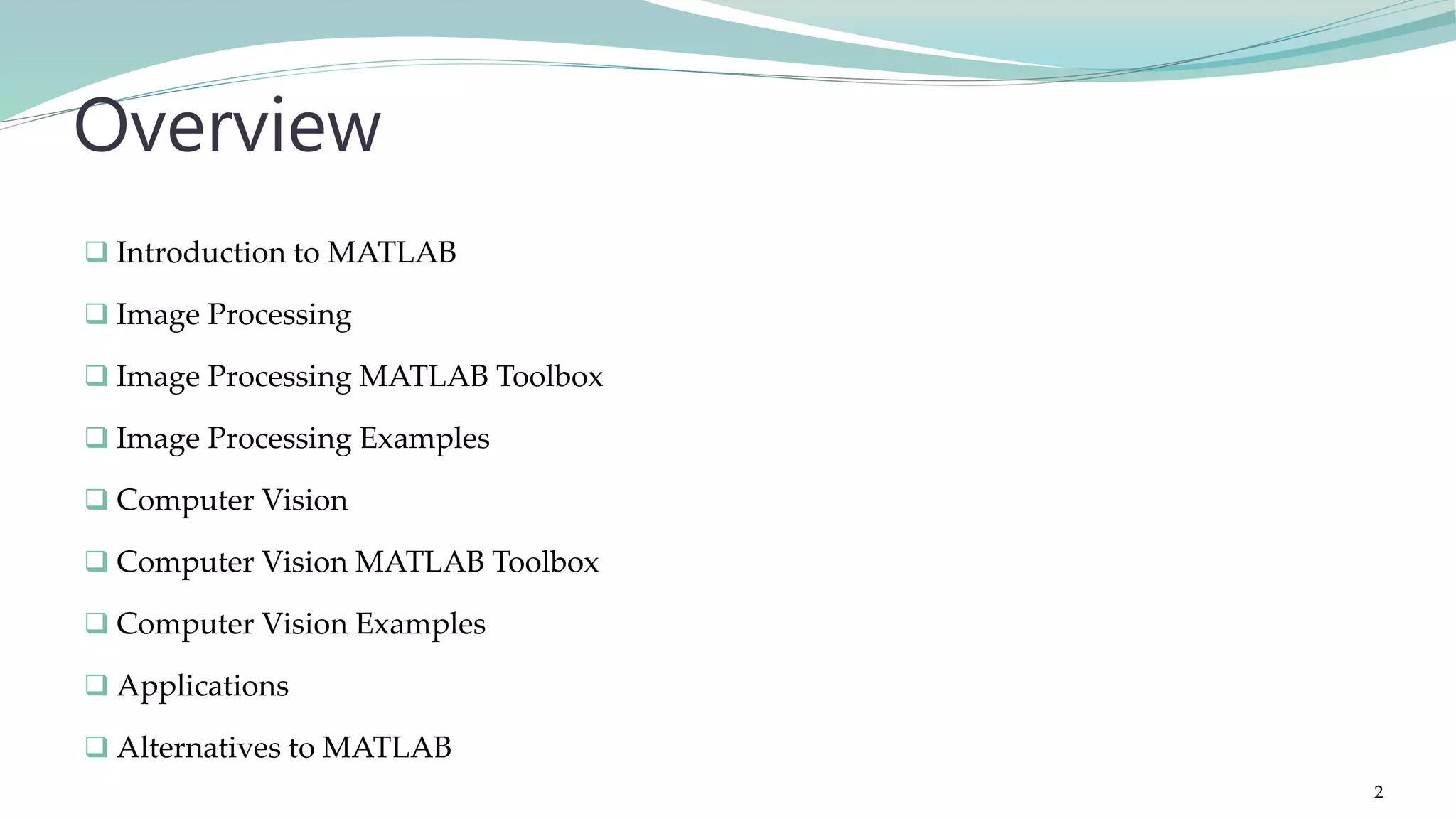
The document provides a comprehensive introduction to MATLAB including its user interface and basic functionalities such as matrix manipulations, plotting, and algorithm implementation. It covers various topics such as image processing and computer vision, explaining the use of MATLAB toolboxes for image analysis, enhancement, and segmentation techniques. Additionally, it discusses advanced topics like calculus, functions, and filtering processes in image processing, along with practical examples and code snippets.

![>> m(3)
ans =
3
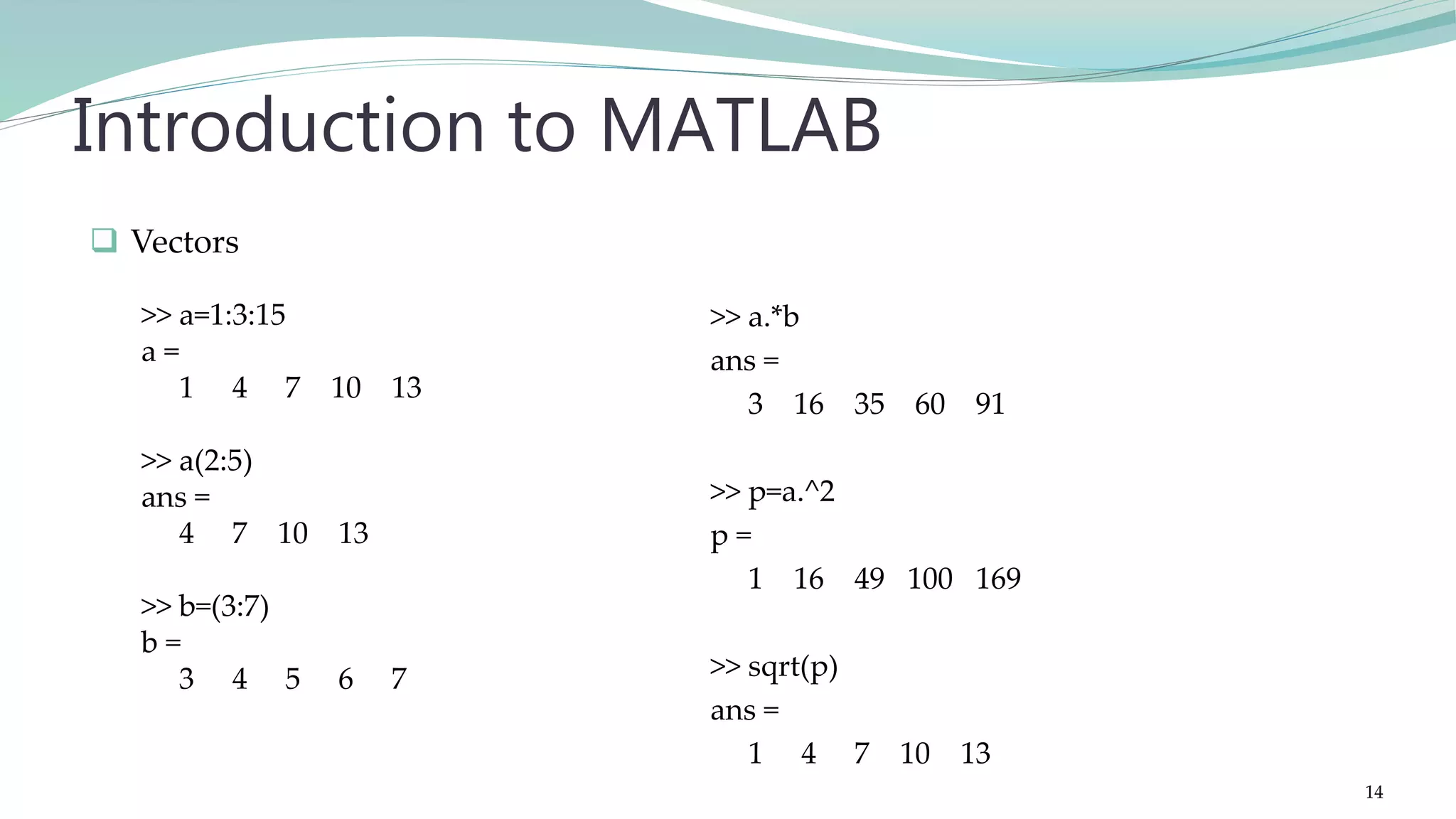
>> length(m)
ans =
5
>> sum(m)
ans =
15
Introduction to MATLAB
>> m=[1 2 3 4 5]
m =
1 2 3 4 5
>> m'
ans =
1
2
3
4
5
>> min(m)
ans =
1
>> max(m)
ans =
5
>> mean(m)
ans =
3
Vectors
13](https://image.slidesharecdn.com/imageprocessingcomputervisionwithmatlab-170402164022/75/Fundamentals-of-Image-Processing-Computer-Vision-with-MATLAB-13-2048.jpg)
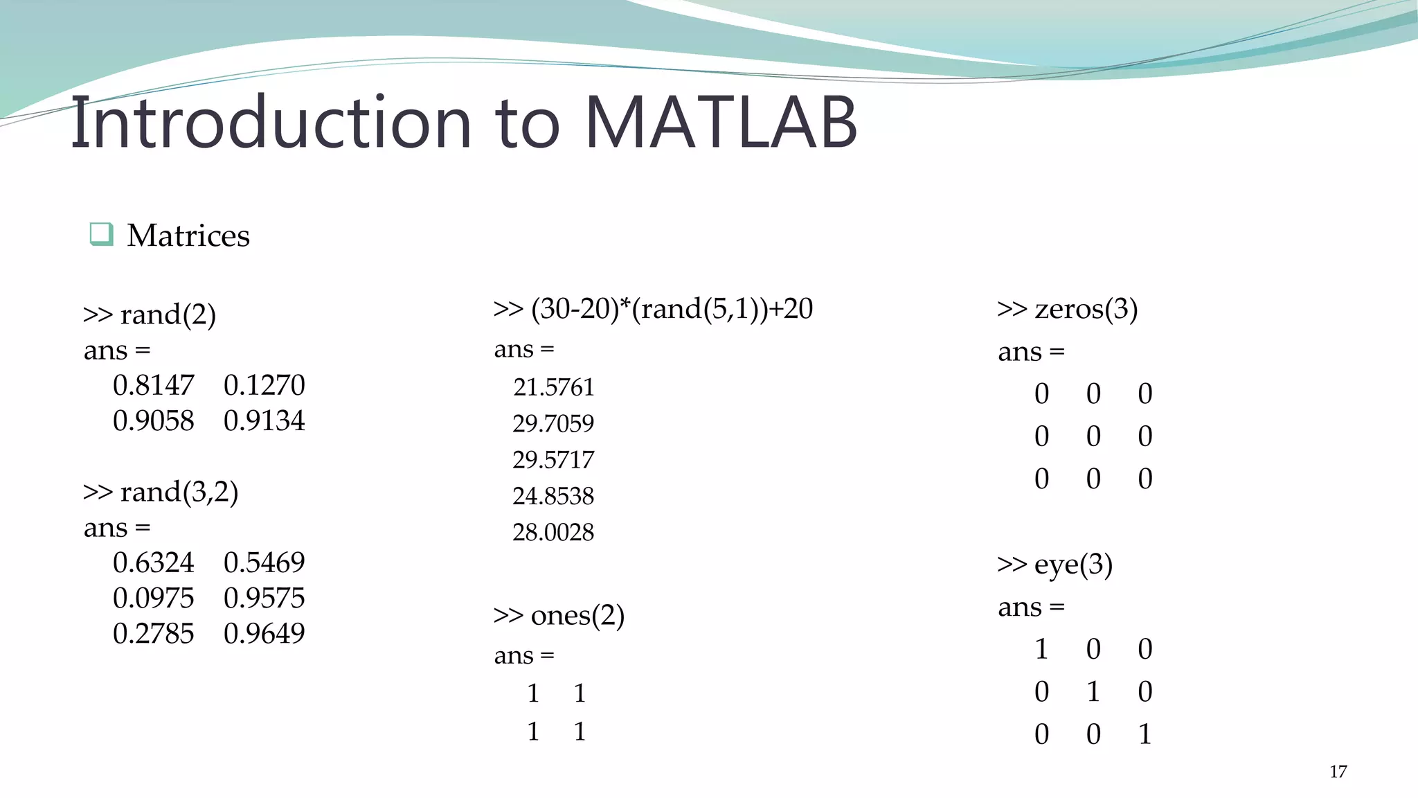
![>> n(2,3)
ans =
4
>> n(3,:)
ans =
7 8 6
>> max(n)
ans =
7 9 6
Introduction to MATLAB
>> min(n)
ans =
2 5 1
>> sum(n)
ans =
12 22 11
>> sum(sum(n))
ans =
45
Matrices
>> n=[3 5 1;2 9 4;7 8 6]
n =
3 5 1
2 9 4
7 8 6
>> n(1:3,2:3)
ans =
5 1
9 4
8 6
15](https://image.slidesharecdn.com/imageprocessingcomputervisionwithmatlab-170402164022/75/Fundamentals-of-Image-Processing-Computer-Vision-with-MATLAB-15-2048.jpg)

![>> std(data)
ans =
26.0109
>> var(data)
ans =
676.5667
Introduction to MATLAB
Statistics
>> data=[12,54,23,69,31,76]
data =
12 54 23 69 31 76
>> sort(data)
ans =
12 23 31 54 69 76
>> median(ans)
ans =
42.5000
18](https://image.slidesharecdn.com/imageprocessingcomputervisionwithmatlab-170402164022/75/Fundamentals-of-Image-Processing-Computer-Vision-with-MATLAB-18-2048.jpg)
![Plotting
>> x=[4 6 8 11 12];
>> y=[1 3 3 5 7];
>> plot(x,y)
>> bar(y)
>> pie(x)
Introduction to MATLAB
24](https://image.slidesharecdn.com/imageprocessingcomputervisionwithmatlab-170402164022/75/Fundamentals-of-Image-Processing-Computer-Vision-with-MATLAB-24-2048.jpg)
![input
>> a=input('enter value for array: ')
enter value for array: [3 4 9 0 2]
a =
3 4 9 0 2
Introduction to MATLAB
>> name=input('enter your name: ','s')
enter your name: Ali
name =
Ali
>> whos
Name Size Bytes Class
name 1x19 38 char
25](https://image.slidesharecdn.com/imageprocessingcomputervisionwithmatlab-170402164022/75/Fundamentals-of-Image-Processing-Computer-Vision-with-MATLAB-25-2048.jpg)
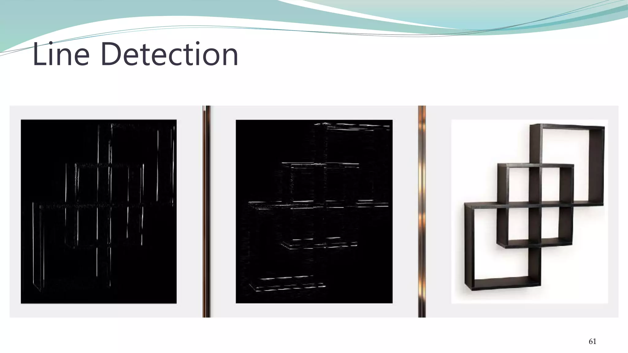
![clc; clear;
a=imread('shelf.png');
b=rgb2gray(a);
figure; imshow(a);
h=[-1 -1 -1;2 2 2; -1 -1 -1]; %filter for horizontal lines
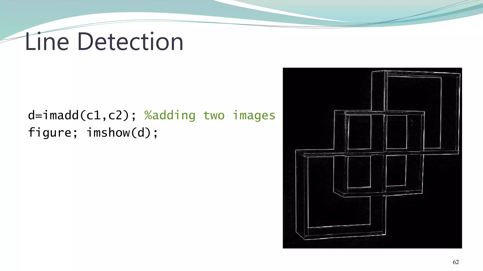
c1=imfilter(b,h);
figure; imshow(c1);
h=[-1 2 -1;-1 2 -1; -1 2 -1]; %filter for vertical lines
c2=imfilter(b,h);
figure; imshow(c2);
Line Detection
60](https://image.slidesharecdn.com/imageprocessingcomputervisionwithmatlab-170402164022/75/Fundamentals-of-Image-Processing-Computer-Vision-with-MATLAB-60-2048.jpg)
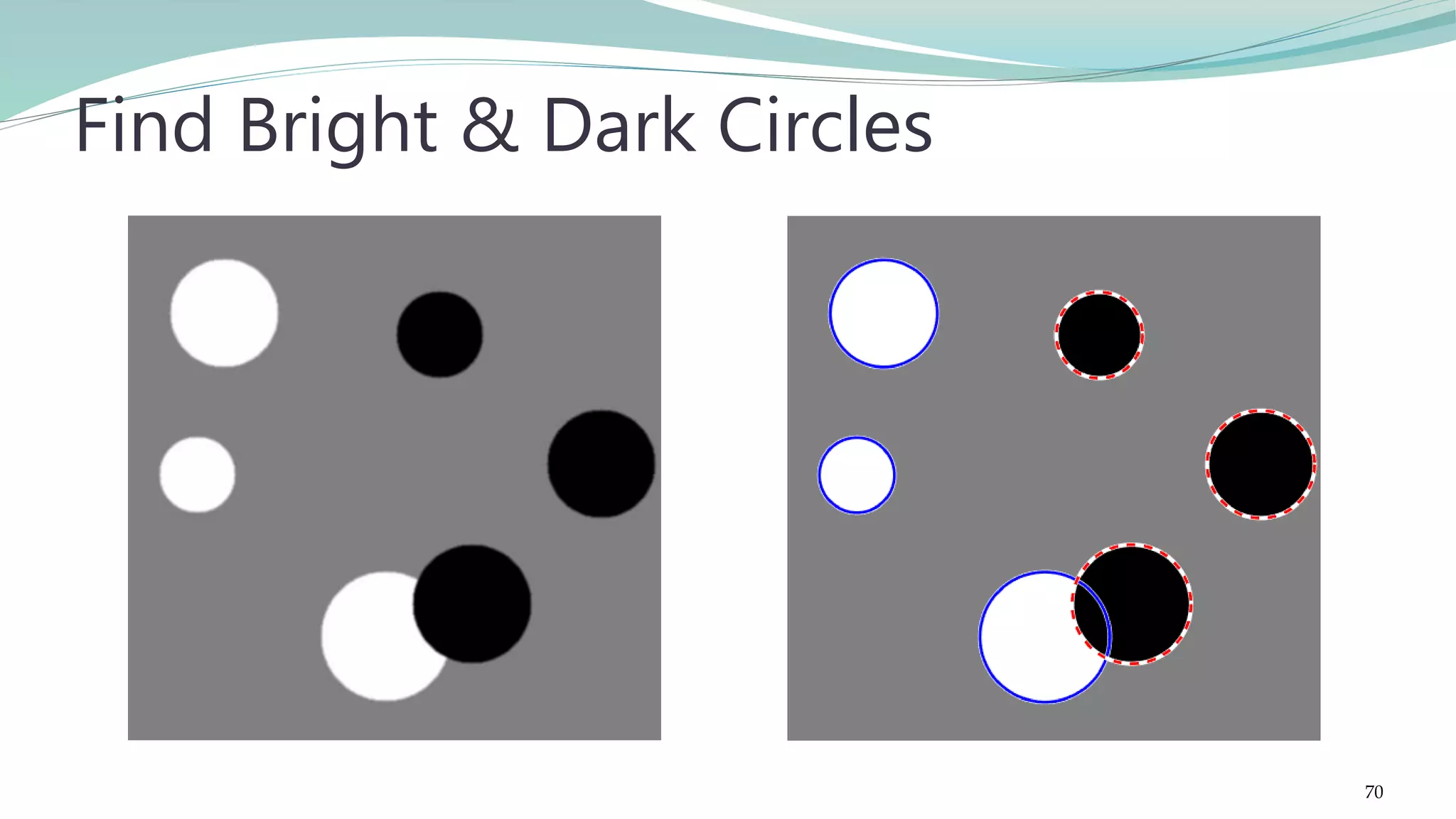
![clc; clear;
A = imread('circlesBrightDark.png');
figure;imshow(A);
Rmin = 30;
Rmax = 65;
[centersBright, radiiBright] = imfindcircles(A,[Rmin …
Rmax],'ObjectPolarity','bright');
[centersDark, radiiDark] = imfindcircles(A,[Rmin …
Rmax],'ObjectPolarity','dark');
figure;imshow(A);
viscircles(centersBright, radiiBright,'EdgeColor','b');
viscircles(centersDark, radiiDark,'LineStyle','--');
Find Bright & Dark Circles
69](https://image.slidesharecdn.com/imageprocessingcomputervisionwithmatlab-170402164022/75/Fundamentals-of-Image-Processing-Computer-Vision-with-MATLAB-69-2048.jpg)

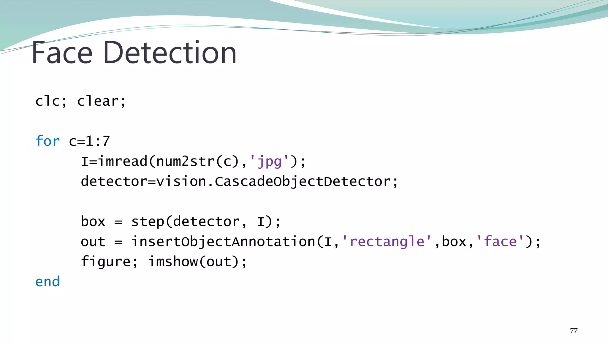
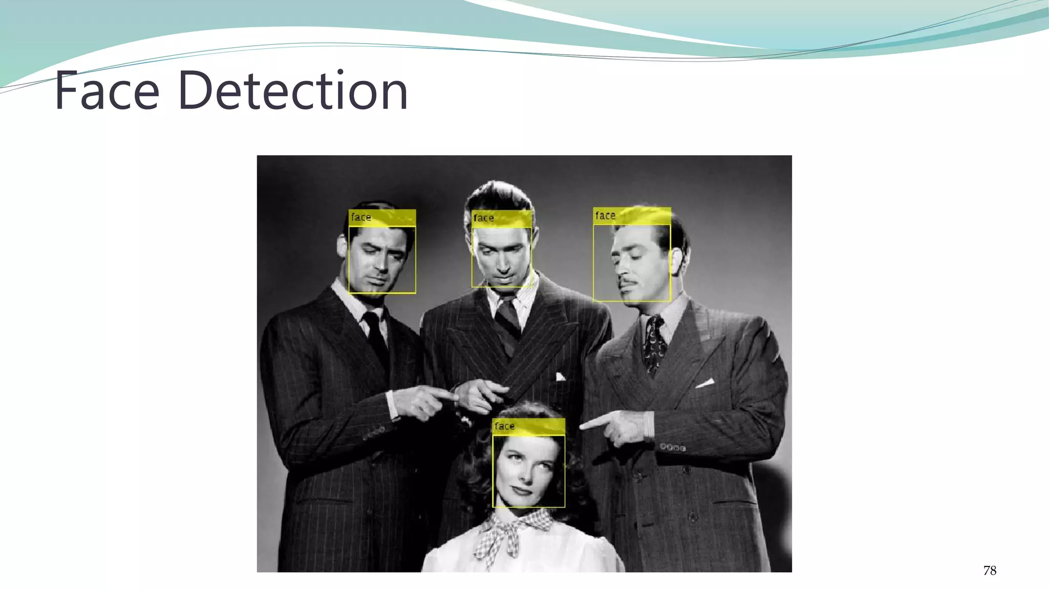
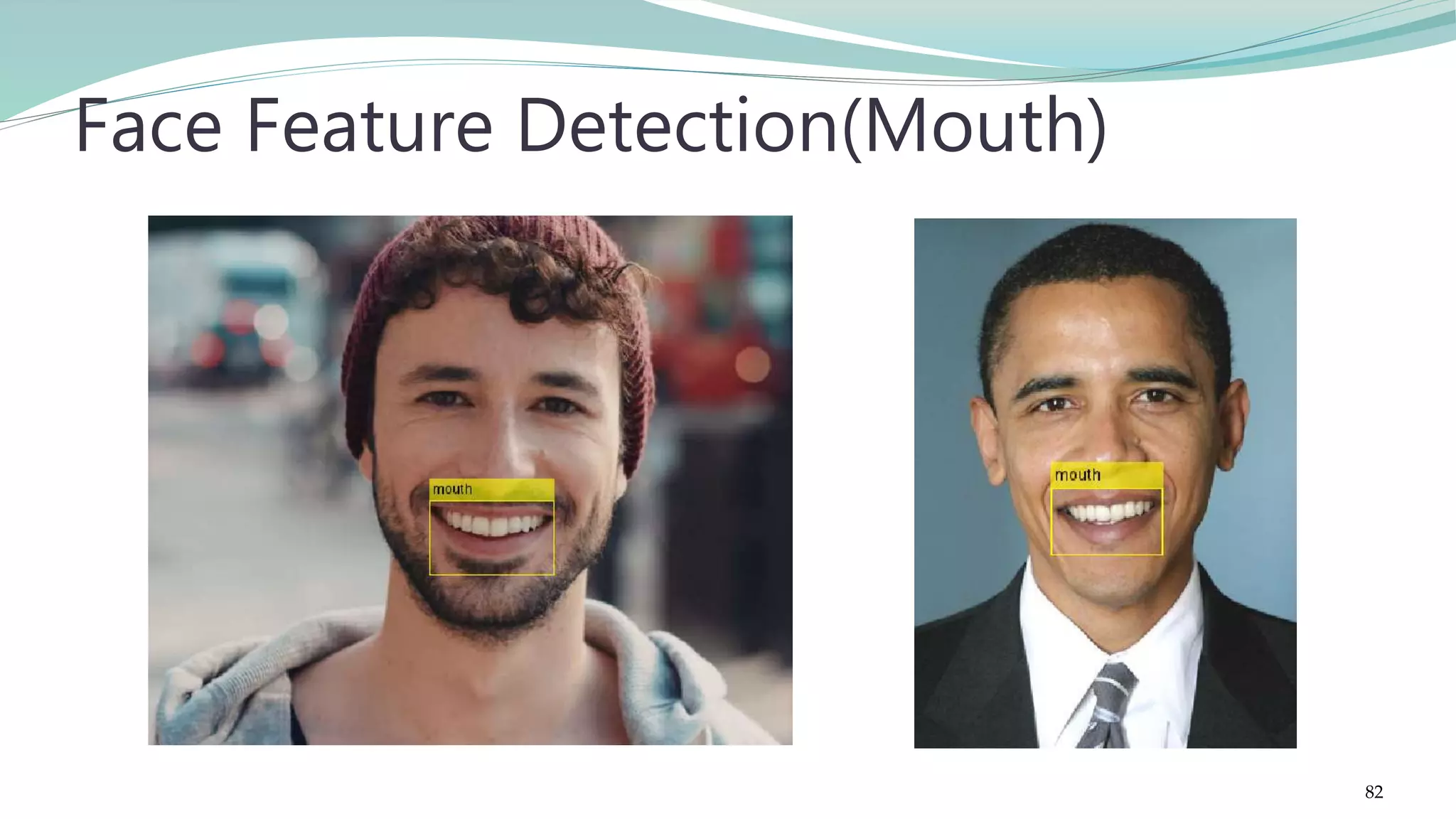
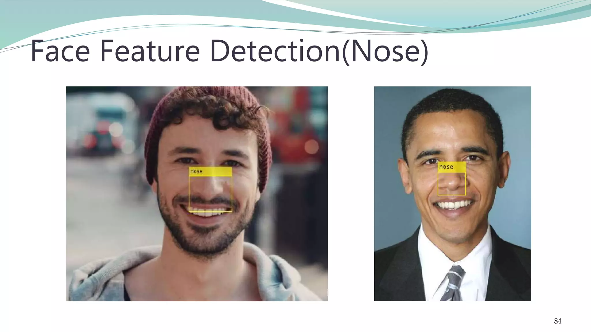
![The cascade object detector uses the Viola-Jones algorithm to detect people's faces,
noses, eyes, mouth, or upper body.
detector = vision.CascadeObjectDetector creates a System object, detector, that
detects objects using the Viola-Jones algorithm. The ClassificationModel property
controls the type of object to detect. By default, the detector is configured to detect
faces.
BBOX = step(detector,I) returns BBOX, an M-by-4 matrix defining M bounding boxes
containing the detected objects. This method performs multiscale object detection on
the input image, I. Each row of the output matrix, BBOX, contains a four-element
vector, [x y width height], that specifies in pixels, the upper-left corner and size of a
bounding box. The input image I, must be a grayscale or truecolor (RGB) image.
Cascade Object Detection
76](https://image.slidesharecdn.com/imageprocessingcomputervisionwithmatlab-170402164022/75/Fundamentals-of-Image-Processing-Computer-Vision-with-MATLAB-76-2048.jpg)
![clc; clear;
faceDetector = vision.CascadeObjectDetector();
obj =imaq.VideoDevice('winvideo', 1, 'YUY2_640x480','ROI', …
[1 1 640 480]);
set(obj,'ReturnedColorSpace', 'rgb');
figure('menubar','none','tag','webcam');
Face Detection from live video stream
86](https://image.slidesharecdn.com/imageprocessingcomputervisionwithmatlab-170402164022/75/Fundamentals-of-Image-Processing-Computer-Vision-with-MATLAB-86-2048.jpg)
![while (true)
frame=step(obj);
bbox=step(faceDetector,frame);
boxInserter =
vision.ShapeInserter('BorderColor','Custom',...
'CustomBorderColor',[255 255 0]);
videoOut = step(boxInserter, frame,bbox);
imshow(videoOut,'border','tight');
f=findobj('tag','webcam');
Face Detection from live video stream
87](https://image.slidesharecdn.com/imageprocessingcomputervisionwithmatlab-170402164022/75/Fundamentals-of-Image-Processing-Computer-Vision-with-MATLAB-87-2048.jpg)
![if (isempty(f));
[hueChannel,~,~] = rgb2hsv(frame);
hold off
noseDetector = vision.CascadeObjectDetector('Nose');
faceImage = imcrop(frame,bbox);
noseBBox = step(noseDetector,faceImage);
videoInfo = info(obj);
ROI=get(obj,'ROI');
VideoSize = [ROI(3) ROI(4)];
tracker = vision.HistogramBasedTracker;
initializeObject(tracker, hueChannel, bbox);
release(obj);
close(gcf)
break
end % End of if
pause(0.05)
end % End of While
Face Detection from live video stream
88](https://image.slidesharecdn.com/imageprocessingcomputervisionwithmatlab-170402164022/75/Fundamentals-of-Image-Processing-Computer-Vision-with-MATLAB-88-2048.jpg)


![>> m(3)
ans =
3
>> length(m)
ans =
5
>> sum(m)
ans =
15
Introduction to MATLAB
>> m=[1 2 3 4 5]
m =
1 2 3 4 5
>> m'
ans =
1
2
3
4
5
>> min(m)
ans =
1
>> max(m)
ans =
5
>> mean(m)
ans =
3
Vectors
13](https://crownmelresort.com/image.slidesharecdn.com/imageprocessingcomputervisionwithmatlab-170402164022/75/Fundamentals-of-Image-Processing-Computer-Vision-with-MATLAB-13-2048.jpg)

![>> n(2,3)
ans =
4
>> n(3,:)
ans =
7 8 6
>> max(n)
ans =
7 9 6
Introduction to MATLAB
>> min(n)
ans =
2 5 1
>> sum(n)
ans =
12 22 11
>> sum(sum(n))
ans =
45
Matrices
>> n=[3 5 1;2 9 4;7 8 6]
n =
3 5 1
2 9 4
7 8 6
>> n(1:3,2:3)
ans =
5 1
9 4
8 6
15](https://crownmelresort.com/image.slidesharecdn.com/imageprocessingcomputervisionwithmatlab-170402164022/75/Fundamentals-of-Image-Processing-Computer-Vision-with-MATLAB-15-2048.jpg)


![>> std(data)
ans =
26.0109
>> var(data)
ans =
676.5667
Introduction to MATLAB
Statistics
>> data=[12,54,23,69,31,76]
data =
12 54 23 69 31 76
>> sort(data)
ans =
12 23 31 54 69 76
>> median(ans)
ans =
42.5000
18](https://crownmelresort.com/image.slidesharecdn.com/imageprocessingcomputervisionwithmatlab-170402164022/75/Fundamentals-of-Image-Processing-Computer-Vision-with-MATLAB-18-2048.jpg)


![Plotting
>> x=[4 6 8 11 12];
>> y=[1 3 3 5 7];
>> plot(x,y)
>> bar(y)
>> pie(x)
Introduction to MATLAB
24](https://crownmelresort.com/image.slidesharecdn.com/imageprocessingcomputervisionwithmatlab-170402164022/75/Fundamentals-of-Image-Processing-Computer-Vision-with-MATLAB-24-2048.jpg)
![input
>> a=input('enter value for array: ')
enter value for array: [3 4 9 0 2]
a =
3 4 9 0 2
Introduction to MATLAB
>> name=input('enter your name: ','s')
enter your name: Ali
name =
Ali
>> whos
Name Size Bytes Class
name 1x19 38 char
25](https://crownmelresort.com/image.slidesharecdn.com/imageprocessingcomputervisionwithmatlab-170402164022/75/Fundamentals-of-Image-Processing-Computer-Vision-with-MATLAB-25-2048.jpg)


![clc; clear;
a=imread('shelf.png');
b=rgb2gray(a);
figure; imshow(a);
h=[-1 -1 -1;2 2 2; -1 -1 -1]; %filter for horizontal lines
c1=imfilter(b,h);
figure; imshow(c1);
h=[-1 2 -1;-1 2 -1; -1 2 -1]; %filter for vertical lines
c2=imfilter(b,h);
figure; imshow(c2);
Line Detection
60](https://crownmelresort.com/image.slidesharecdn.com/imageprocessingcomputervisionwithmatlab-170402164022/75/Fundamentals-of-Image-Processing-Computer-Vision-with-MATLAB-60-2048.jpg)


![clc; clear;
A = imread('circlesBrightDark.png');
figure;imshow(A);
Rmin = 30;
Rmax = 65;
[centersBright, radiiBright] = imfindcircles(A,[Rmin …
Rmax],'ObjectPolarity','bright');
[centersDark, radiiDark] = imfindcircles(A,[Rmin …
Rmax],'ObjectPolarity','dark');
figure;imshow(A);
viscircles(centersBright, radiiBright,'EdgeColor','b');
viscircles(centersDark, radiiDark,'LineStyle','--');
Find Bright & Dark Circles
69](https://crownmelresort.com/image.slidesharecdn.com/imageprocessingcomputervisionwithmatlab-170402164022/75/Fundamentals-of-Image-Processing-Computer-Vision-with-MATLAB-69-2048.jpg)


![The cascade object detector uses the Viola-Jones algorithm to detect people's faces,
noses, eyes, mouth, or upper body.
detector = vision.CascadeObjectDetector creates a System object, detector, that
detects objects using the Viola-Jones algorithm. The ClassificationModel property
controls the type of object to detect. By default, the detector is configured to detect
faces.
BBOX = step(detector,I) returns BBOX, an M-by-4 matrix defining M bounding boxes
containing the detected objects. This method performs multiscale object detection on
the input image, I. Each row of the output matrix, BBOX, contains a four-element
vector, [x y width height], that specifies in pixels, the upper-left corner and size of a
bounding box. The input image I, must be a grayscale or truecolor (RGB) image.
Cascade Object Detection
76](https://crownmelresort.com/image.slidesharecdn.com/imageprocessingcomputervisionwithmatlab-170402164022/75/Fundamentals-of-Image-Processing-Computer-Vision-with-MATLAB-76-2048.jpg)


![clc; clear;
faceDetector = vision.CascadeObjectDetector();
obj =imaq.VideoDevice('winvideo', 1, 'YUY2_640x480','ROI', …
[1 1 640 480]);
set(obj,'ReturnedColorSpace', 'rgb');
figure('menubar','none','tag','webcam');
Face Detection from live video stream
86](https://crownmelresort.com/image.slidesharecdn.com/imageprocessingcomputervisionwithmatlab-170402164022/75/Fundamentals-of-Image-Processing-Computer-Vision-with-MATLAB-86-2048.jpg)
![while (true)
frame=step(obj);
bbox=step(faceDetector,frame);
boxInserter =
vision.ShapeInserter('BorderColor','Custom',...
'CustomBorderColor',[255 255 0]);
videoOut = step(boxInserter, frame,bbox);
imshow(videoOut,'border','tight');
f=findobj('tag','webcam');
Face Detection from live video stream
87](https://crownmelresort.com/image.slidesharecdn.com/imageprocessingcomputervisionwithmatlab-170402164022/75/Fundamentals-of-Image-Processing-Computer-Vision-with-MATLAB-87-2048.jpg)
![if (isempty(f));
[hueChannel,~,~] = rgb2hsv(frame);
hold off
noseDetector = vision.CascadeObjectDetector('Nose');
faceImage = imcrop(frame,bbox);
noseBBox = step(noseDetector,faceImage);
videoInfo = info(obj);
ROI=get(obj,'ROI');
VideoSize = [ROI(3) ROI(4)];
tracker = vision.HistogramBasedTracker;
initializeObject(tracker, hueChannel, bbox);
release(obj);
close(gcf)
break
end % End of if
pause(0.05)
end % End of While
Face Detection from live video stream
88](https://crownmelresort.com/image.slidesharecdn.com/imageprocessingcomputervisionwithmatlab-170402164022/75/Fundamentals-of-Image-Processing-Computer-Vision-with-MATLAB-88-2048.jpg)