Downloaded 85 times
![General Form of Newton’s Interpolating
Polynomials
)()(
],[
ji
ji
ji
xx
xfxf
xxf
Bracketed function
evaluations are finite
divided differences
],,,,[],,[],[)(
)())(())(()()(
011012201100
110102010
xxxxfbxxxfbxxfbxfb
xxxxxxbxxxxbxxbbxf
nnn
nnn
],[],[
],,[
ki
kjji
kji
xx
xxfxxf
xxxf
0
02111
011
xx
xxxfxxxf
xxxxf
n
nnnn
nn
],,,[],,,[
],,,,[
](https://image.slidesharecdn.com/interpolation-190605141327/75/Interpolation-8-2048.jpg)
![xi f(xi)
x0 f(x0)
x1 f(x1)
x2 f(x2)
x3 f(x3)
x4 f(x4)
xi f(xi)
x0=0 2
x1=2 14
x2=3 74
x3=4 242
x4=5 602
f1(x) = 2 + 6*(x-0) (based on x0 and x1)
f2(x) = 2 + 6*(x-0)+18(x-0)(x-2) (based on x0, x1 and x2)
f3(x) = 2 + 6*(x-0)+18(x-0)(x-2)+9(x-0)(x-2)(x-3) (based on x0, x1, x2, and x3)
f4(x) = 2 + 6x +18x(x-2) +9x(x-2)(x-3) +1x(x-2)(x-3)(x-4) (based on x0, x1, x2, x3, and x4)
= x4 – x2 + 2
EXAMPLEDIVIDED DIFFERENCE TABLE
f[xi,xj]
6
60
168
360
f[xi,xj,xk]
18
54
96
f[x,x,x,x]
9
14
f[x...x]
1
f[xi,xj]
f[x1,x0]
f[x2,x1]
f[x3,x2]
f[x4,x3]
f[xi,xj,xk]
f[x2,x1,x0]
f[x3,x2,x1]
f[x4,x3,x2]
f[x,x,x,x]
f[x3,x2,x1,x0]
f[x4,x3,x2,x1]](https://image.slidesharecdn.com/interpolation-190605141327/75/Interpolation-9-2048.jpg)
![Given:
x0=1 f(x0)=ln(1) = 0
x1=e f(x1)=ln(2.72) = 1
x2=e2 f(x2)=ln(7.39) = 2
Estimate ln(2) = ?
using interpolation
Find f(x) first
xi f(xi)
x0=1 0
x1=2.72 1
x2=7.39 2
f[xi,xj]
.58
.214
f[xi,xj xk]
-.057
f(x) = 0.58(x-1)
-0.057(x-1)(x-
2.72)
Then calculate
f(2)=0.58(2-1)-0.057(2-1)(2-
2.72)
= 0.621
[ TRUE ln(2) = 0.6931 ]
Example](https://image.slidesharecdn.com/interpolation-190605141327/75/Interpolation-10-2048.jpg)
![Image Interpolation - Theory
[IDEA]
In order to provide a richer environment we are thinking of using
interpolation methods that will generate “artificial images” thus revealing
hidden information.
[RADON RECONSTRUCTION]
Radon reconstruction is the technique in which the object is reconstructed
from its projections. This reconstruction method is based on approximating
the inverse Radon Transform.
[RADON Transform]
The 2-D Radon transform is the mathematical relationship which maps the
spatial domain (x,y) to the Radon domain (p,phi). The Radon transform
consists of taking a line integral along a line (ray) which passes through the
object space. The radon transform is expressed mathematically as:
dxdypyxyxpR )sincos(),(),}({ ](https://image.slidesharecdn.com/interpolation-190605141327/75/Interpolation-13-2048.jpg)


![General Form of Newton’s Interpolating
Polynomials
)()(
],[
ji
ji
ji
xx
xfxf
xxf
Bracketed function
evaluations are finite
divided differences
],,,,[],,[],[)(
)())(())(()()(
011012201100
110102010
xxxxfbxxxfbxxfbxfb
xxxxxxbxxxxbxxbbxf
nnn
nnn
],[],[
],,[
ki
kjji
kji
xx
xxfxxf
xxxf
0
02111
011
xx
xxxfxxxf
xxxxf
n
nnnn
nn
],,,[],,,[
],,,,[
](https://crownmelresort.com/image.slidesharecdn.com/interpolation-190605141327/75/Interpolation-8-2048.jpg)
![xi f(xi)
x0 f(x0)
x1 f(x1)
x2 f(x2)
x3 f(x3)
x4 f(x4)
xi f(xi)
x0=0 2
x1=2 14
x2=3 74
x3=4 242
x4=5 602
f1(x) = 2 + 6*(x-0) (based on x0 and x1)
f2(x) = 2 + 6*(x-0)+18(x-0)(x-2) (based on x0, x1 and x2)
f3(x) = 2 + 6*(x-0)+18(x-0)(x-2)+9(x-0)(x-2)(x-3) (based on x0, x1, x2, and x3)
f4(x) = 2 + 6x +18x(x-2) +9x(x-2)(x-3) +1x(x-2)(x-3)(x-4) (based on x0, x1, x2, x3, and x4)
= x4 – x2 + 2
EXAMPLEDIVIDED DIFFERENCE TABLE
f[xi,xj]
6
60
168
360
f[xi,xj,xk]
18
54
96
f[x,x,x,x]
9
14
f[x...x]
1
f[xi,xj]
f[x1,x0]
f[x2,x1]
f[x3,x2]
f[x4,x3]
f[xi,xj,xk]
f[x2,x1,x0]
f[x3,x2,x1]
f[x4,x3,x2]
f[x,x,x,x]
f[x3,x2,x1,x0]
f[x4,x3,x2,x1]](https://crownmelresort.com/image.slidesharecdn.com/interpolation-190605141327/75/Interpolation-9-2048.jpg)
![Given:
x0=1 f(x0)=ln(1) = 0
x1=e f(x1)=ln(2.72) = 1
x2=e2 f(x2)=ln(7.39) = 2
Estimate ln(2) = ?
using interpolation
Find f(x) first
xi f(xi)
x0=1 0
x1=2.72 1
x2=7.39 2
f[xi,xj]
.58
.214
f[xi,xj xk]
-.057
f(x) = 0.58(x-1)
-0.057(x-1)(x-
2.72)
Then calculate
f(2)=0.58(2-1)-0.057(2-1)(2-
2.72)
= 0.621
[ TRUE ln(2) = 0.6931 ]
Example](https://crownmelresort.com/image.slidesharecdn.com/interpolation-190605141327/75/Interpolation-10-2048.jpg)


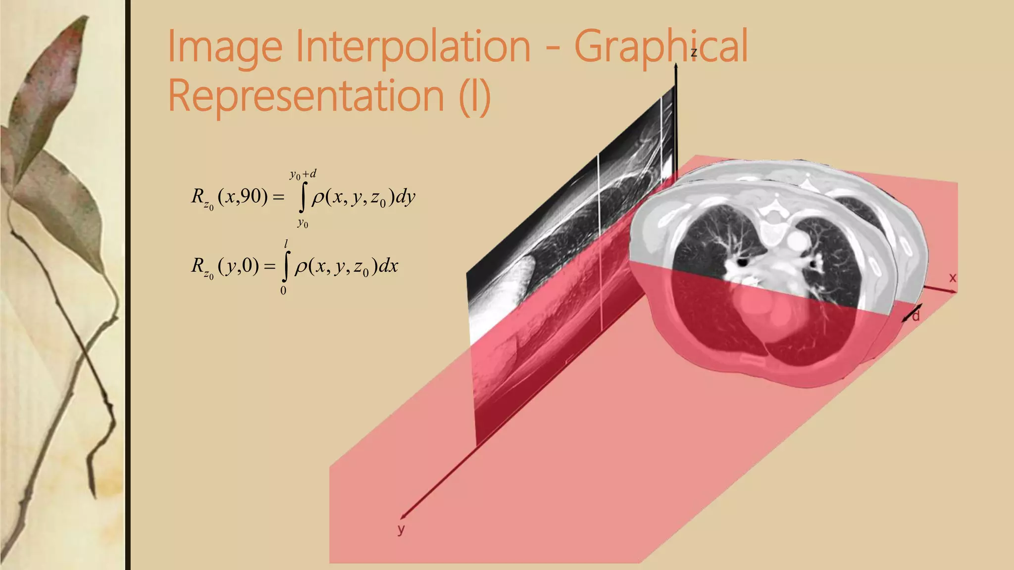
![Image Interpolation - Theory
[IDEA]
In order to provide a richer environment we are thinking of using
interpolation methods that will generate “artificial images” thus revealing
hidden information.
[RADON RECONSTRUCTION]
Radon reconstruction is the technique in which the object is reconstructed
from its projections. This reconstruction method is based on approximating
the inverse Radon Transform.
[RADON Transform]
The 2-D Radon transform is the mathematical relationship which maps the
spatial domain (x,y) to the Radon domain (p,phi). The Radon transform
consists of taking a line integral along a line (ray) which passes through the
object space. The radon transform is expressed mathematically as:
dxdypyxyxpR )sincos(),(),}({ ](https://crownmelresort.com/image.slidesharecdn.com/interpolation-190605141327/75/Interpolation-13-2048.jpg)


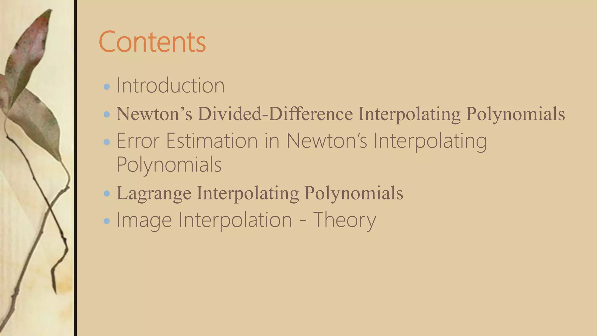
This document discusses various interpolation methods used in numerical analysis and civil engineering. It describes Newton's divided difference interpolation polynomials which use higher order polynomials to fit additional data points. Lagrange interpolation polynomials are also covered, which avoid divided differences by reformulating Newton's method. The document provides examples of applying these techniques. It concludes with an overview of image interpolation theory, describing how the Radon transform maps spatial data to projections that can be reconstructed.
Overview of the presentation on Interpolation as part of Numerical and Statistical Methods for Civil Engineering.
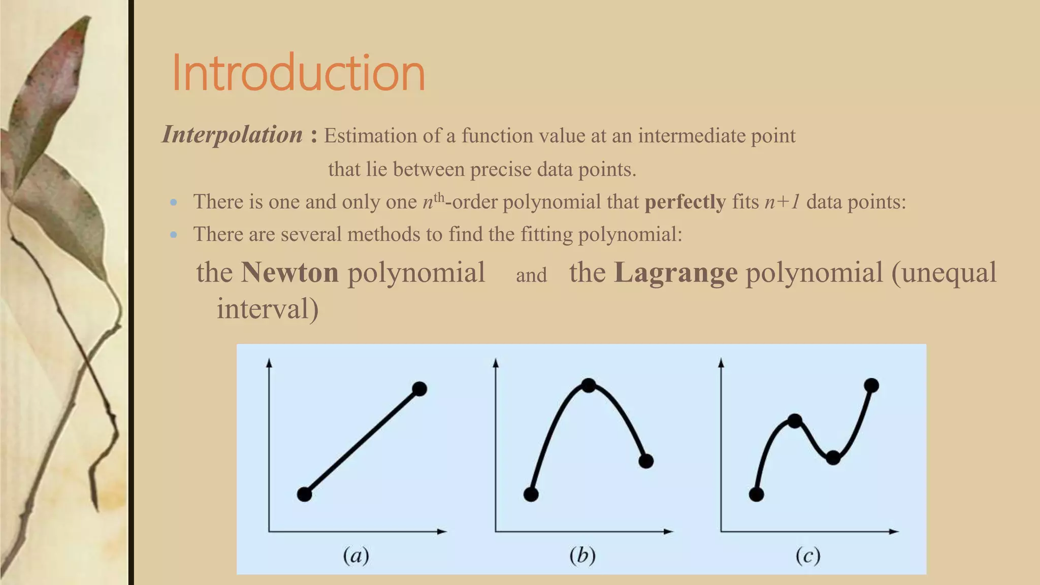
Defines interpolation as estimation of function values between data points, introducing Newton and Lagrange polynomials.
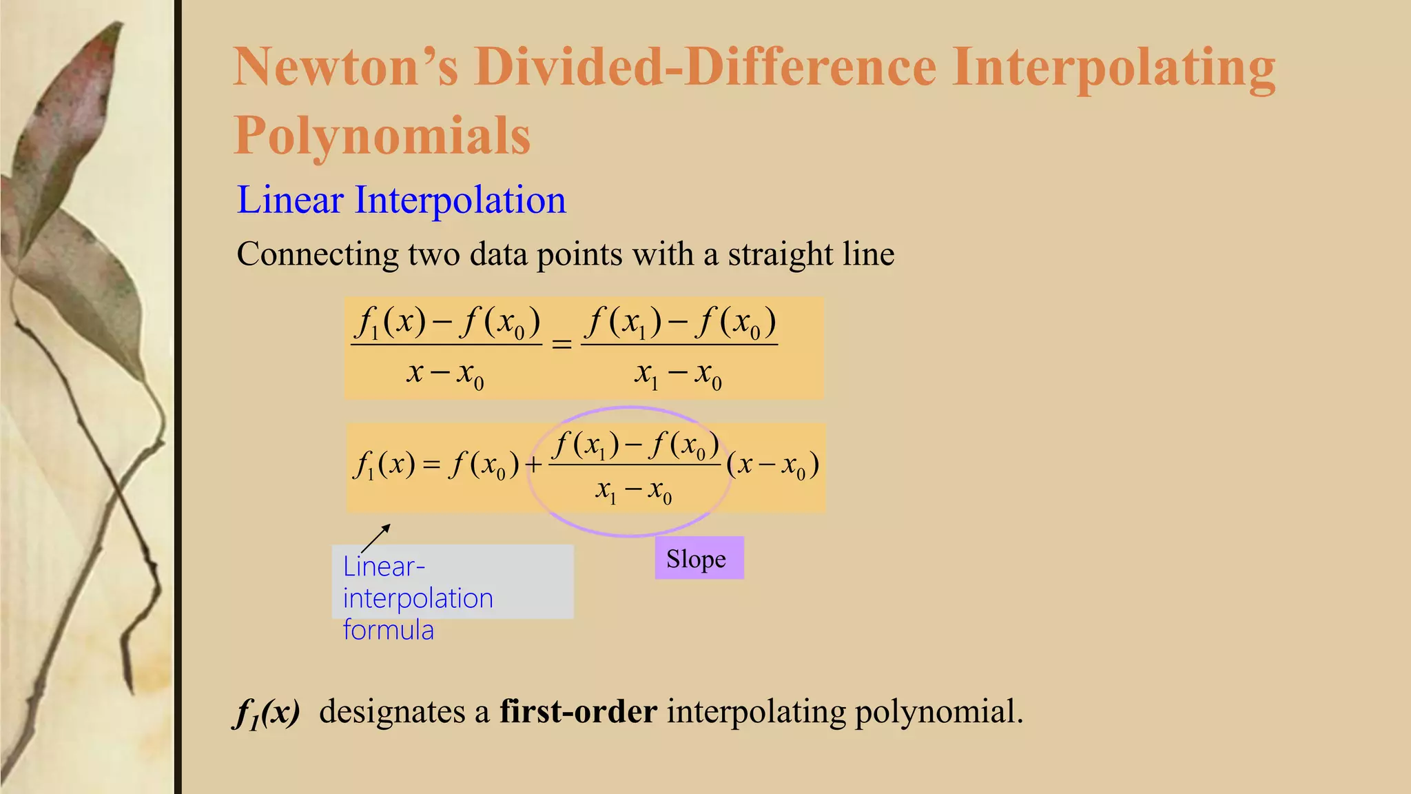
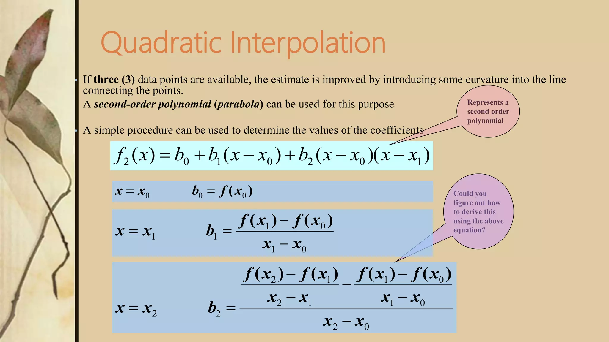
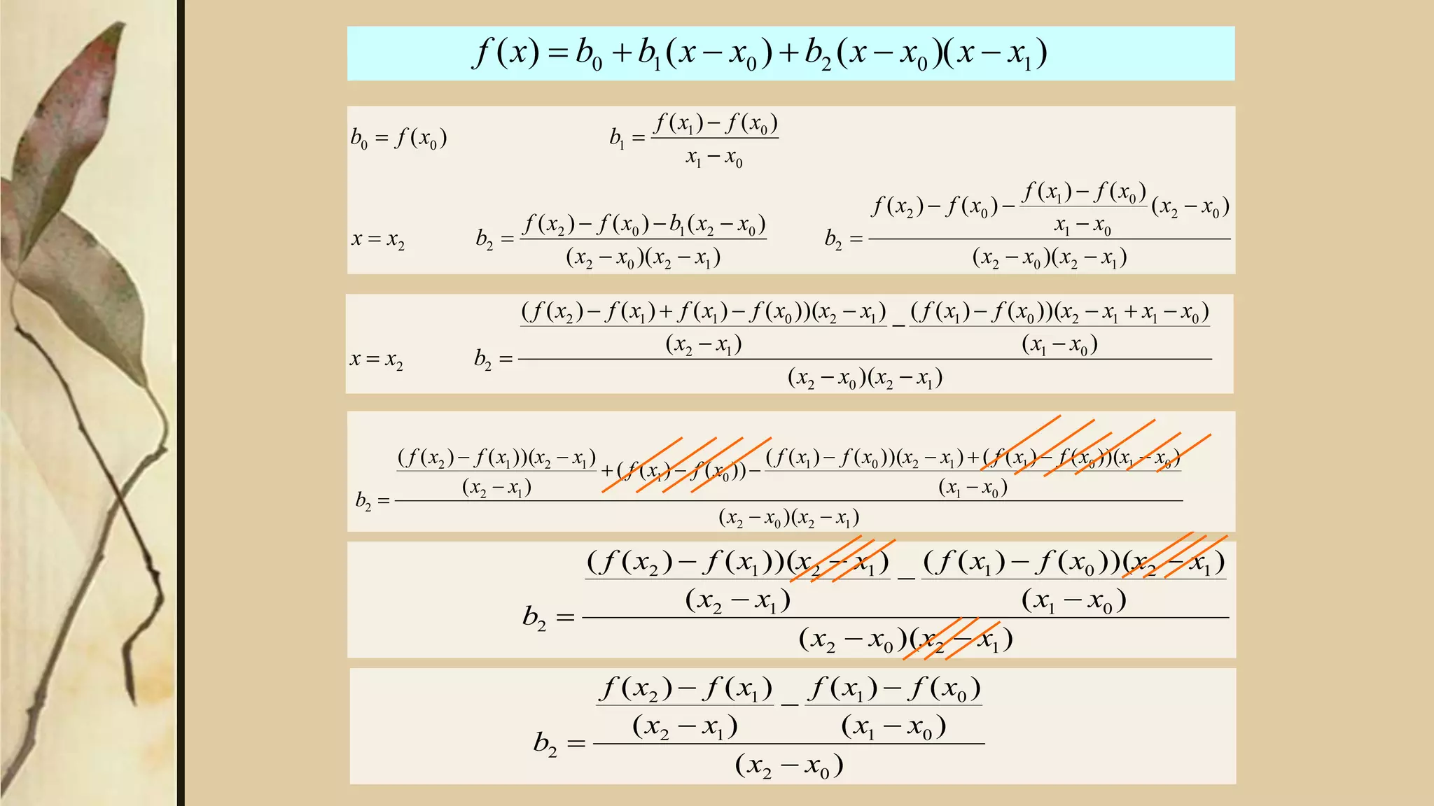
Details on Newton's divided-difference polynomials with linear and quadratic interpolation formulas.
Numerical examples and calculations using Newton's divided difference for estimating function values.
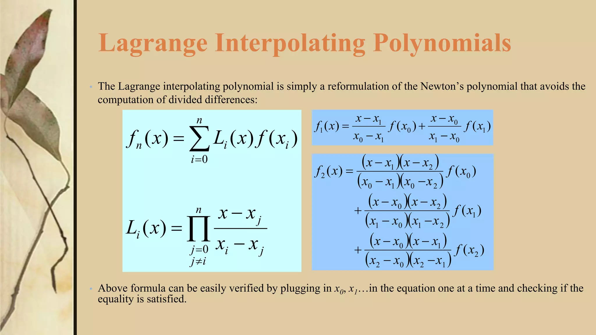
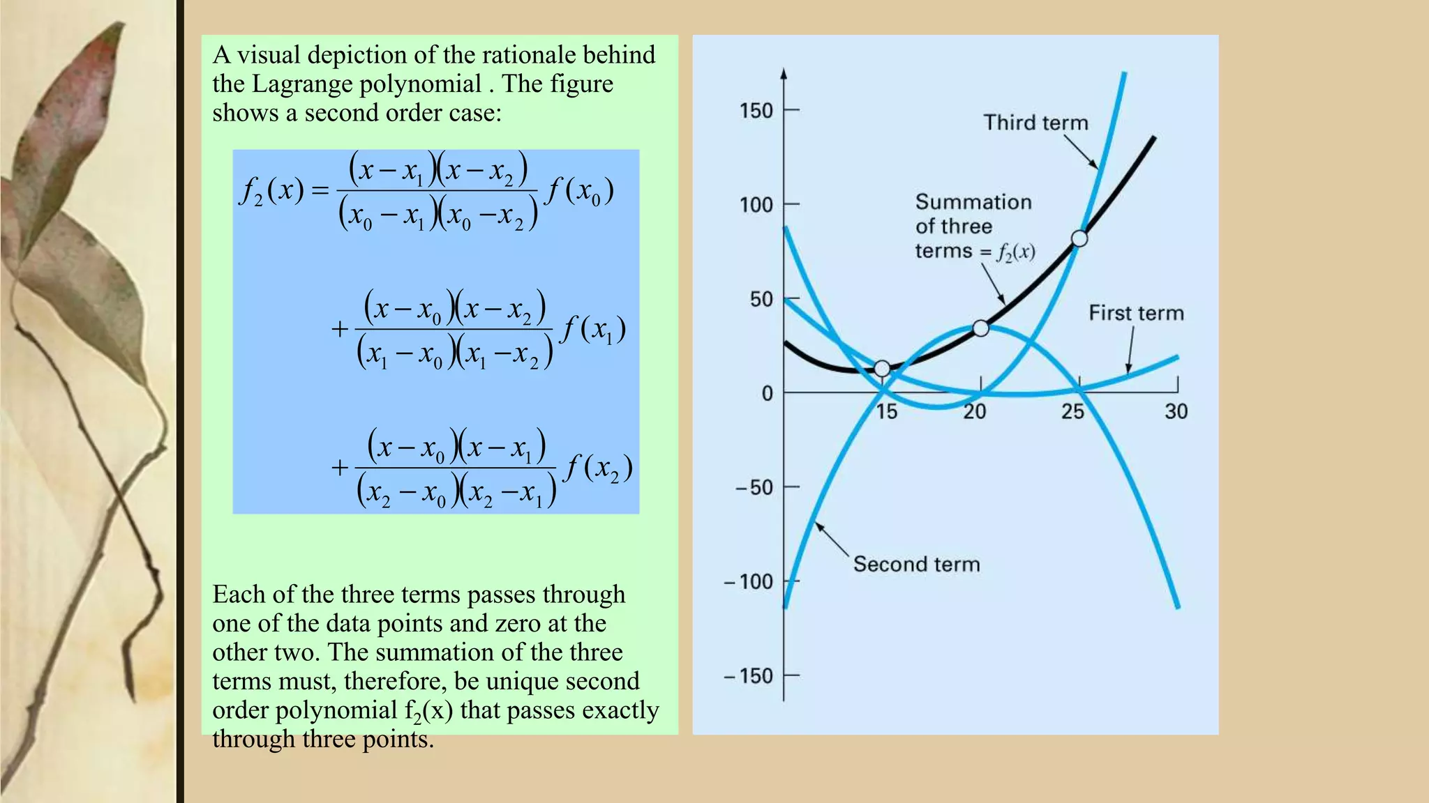
Introduction and visual representation of Lagrange polynomial, emphasizing its relation to Newton's method.
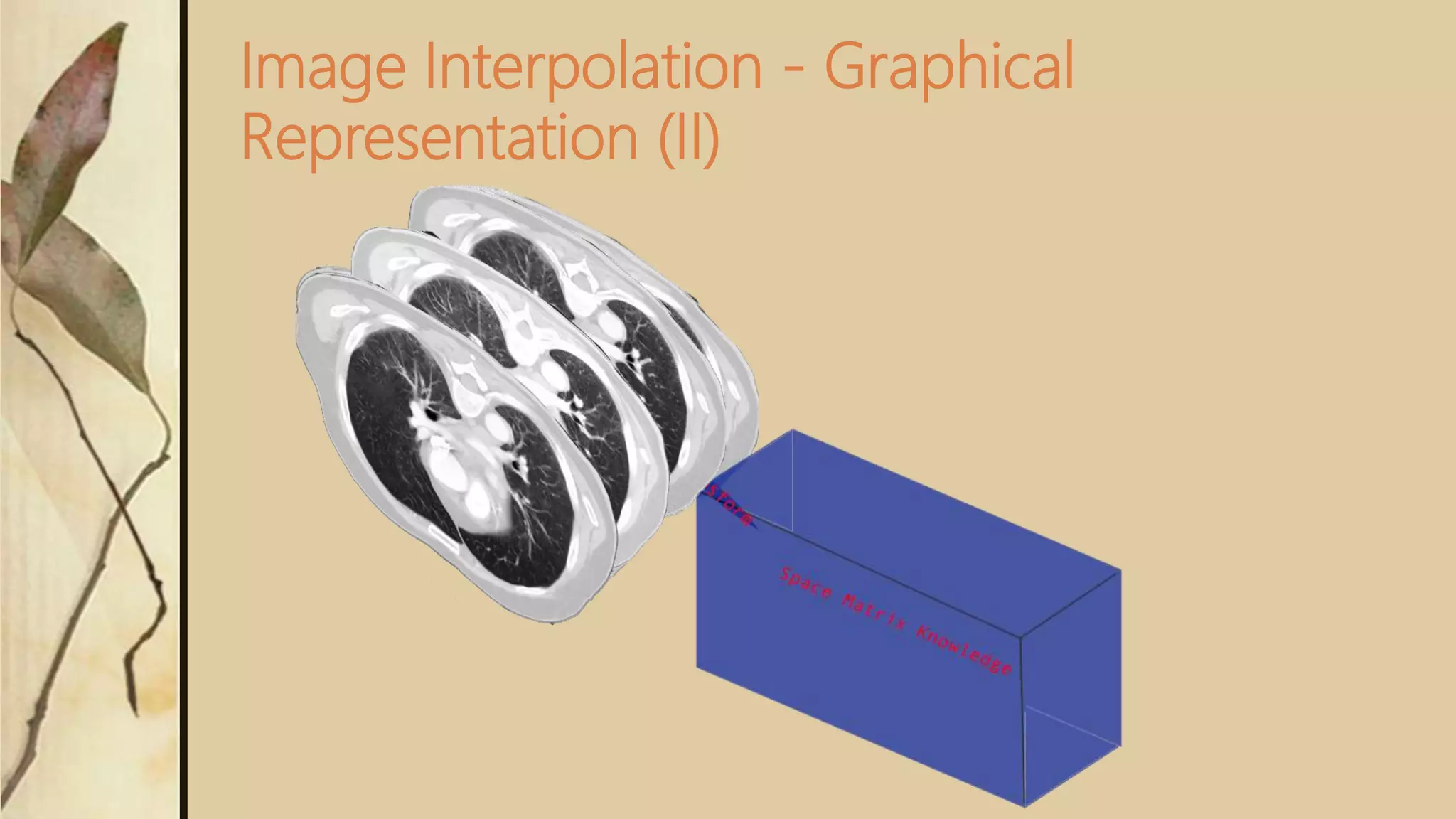
Explores theoretical and graphical aspects of image interpolation, including Radon transform and reconstruction.
Acknowledgment slide listing contributors involved in the presentation.


![ANPARA THERMAL POWER STATION[1] sangam.pdf](https://cdn.slidesharecdn.com/ss_thumbnails/anparathermalpowerstation1sangam-251121115219-9261cde4-thumbnail.jpg?width=640&height=640&fit=bounds)


