Interpolation
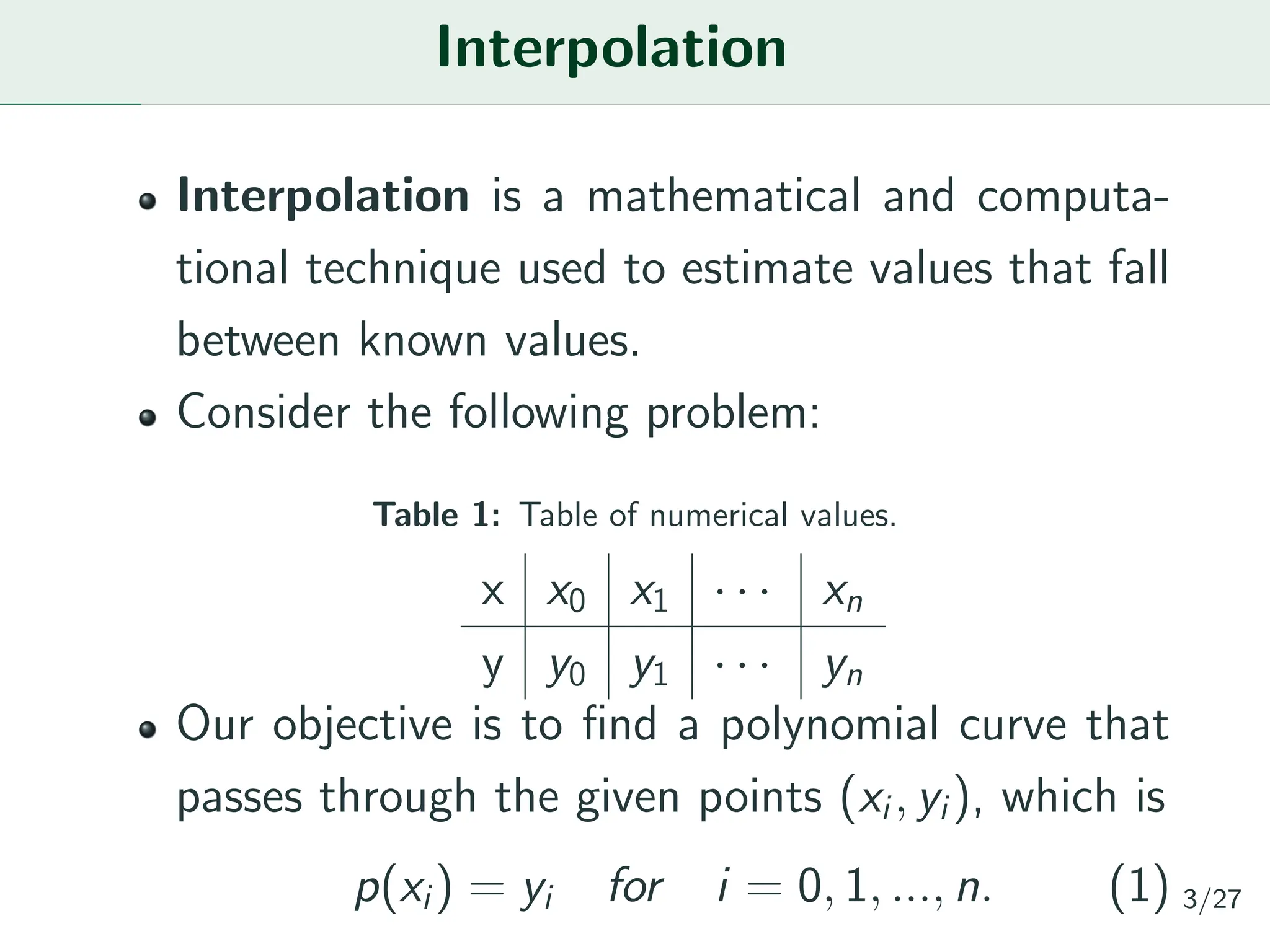
Interpolation is amathematical and computa-
tional technique used to estimate values that fall
between known values.
Consider the following problem:
Table 1: Table of numerical values.
x x0 x1 · · · xn
y y0 y1 · · · yn
Our objective is to find a polynomial curve that
passes through the given points (xi, yi), which is
p(xi) = yi for i = 0, 1, ..., n. (1) 3/27
4.
Polynomial Interpolation Theory
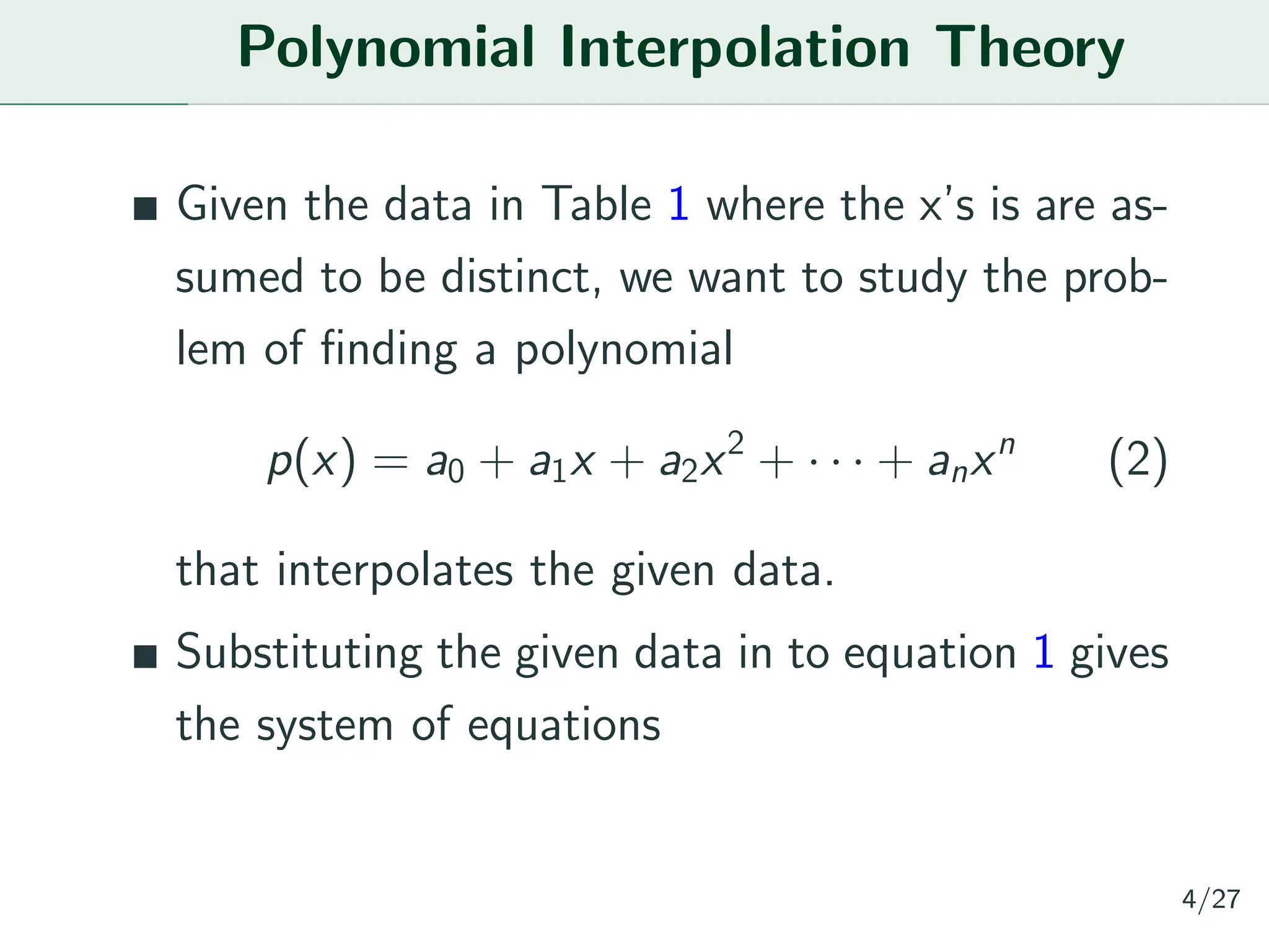
Giventhe data in Table 1 where the x’s is are as-
sumed to be distinct, we want to study the prob-
lem of finding a polynomial
p(x) = a0 + a1x + a2x2
+ · · · + anxn
(2)
that interpolates the given data.
Substituting the given data in to equation 1 gives
the system of equations
4/27
5.
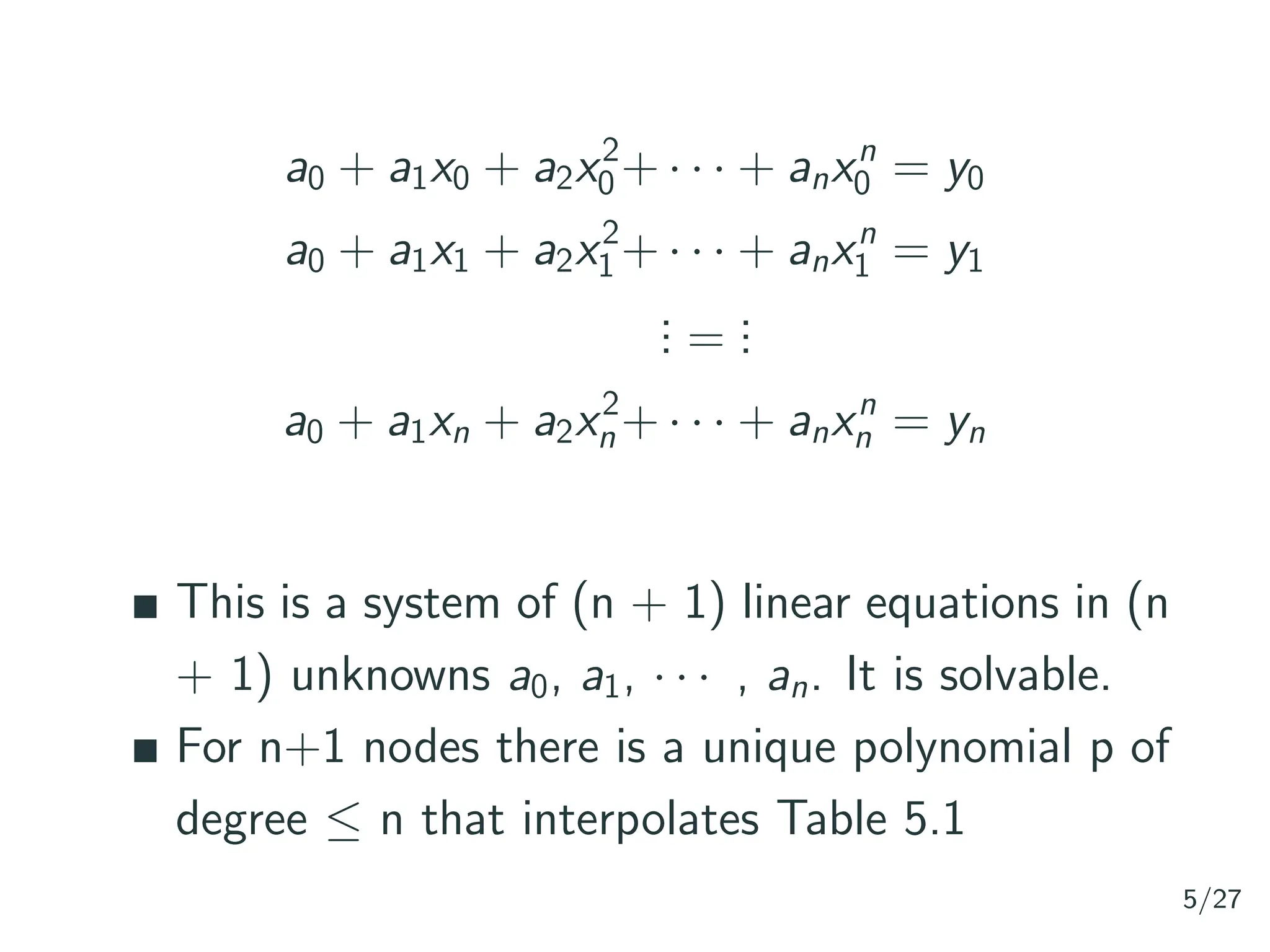
a0 + a1x0+ a2x2
0 + · · · + anxn
0 = y0
a0 + a1x1 + a2x2
1 + · · · + anxn
1 = y1
.
.
. =
.
.
.
a0 + a1xn + a2x2
n + · · · + anxn
n = yn
This is a system of (n + 1) linear equations in (n
+ 1) unknowns a0, a1, · · · , an. It is solvable.
For n+1 nodes there is a unique polynomial p of
degree ≤ n that interpolates Table 5.1
5/27
6.
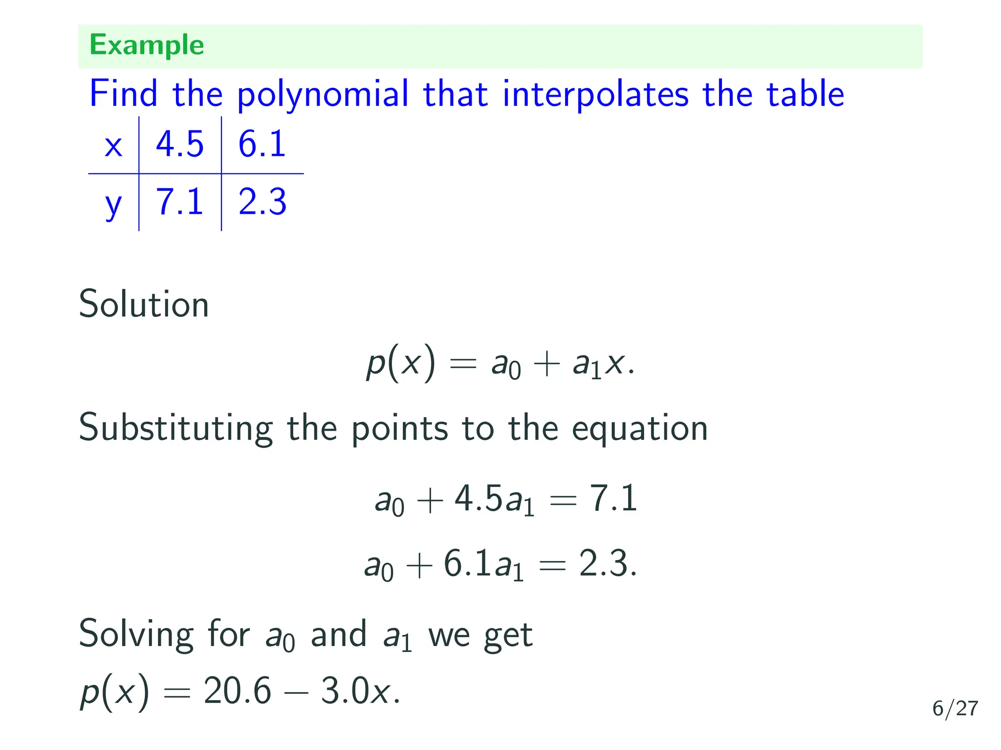
Example
Find the polynomialthat interpolates the table
x 4.5 6.1
y 7.1 2.3
Solution
p(x) = a0 + a1x.
Substituting the points to the equation
a0 + 4.5a1 = 7.1
a0 + 6.1a1 = 2.3.
Solving for a0 and a1 we get
p(x) = 20.6 − 3.0x. 6/27
7.
Newton’s Divided-Difference InterpolatingPolynomial
In this section we want to develop an interpolat-
ing formula that will be more efficient and conve-
nient to use than the one shown in the previous
section
This will avoid the problem of finding the solution
to a system of simultaneous equations.
Pn(x) = f [x0] + f [x0, x1](x − x0)
+f [x0, x1, x2](x − x0)(x − x1)
+ · · · f [x0, x1, x2 · · · , xn](x − x0)(x − x1) · · · (x − xn−1)
7/27
8.
Newton’s Divided-Difference InterpolatingPolynomial
The above equation is know as n-order
newron-divided deference polynomial and where
the notation
f [x0, x1, · · · , xn] =
f [x1, x2, · · · xn] − f [x0, x2, · · · xn−1]
xn − x0
is know as divided-difference
ˆ The first four divided differences denoted as ff
f [x0] = f (x0)
f [x0, x1] =
f [x1] − f [x0]
x1 − x0
8/27
9.
Newton’s Divided-Difference InterpolatingPolynomial
f [x0, x1, x2] =
f [x1, x2] − f [x0, x1]
x2 − x0
f [x0, x1, x2, x3] =
f [x1, x2, x3] − f [x0, x1, x2]
x3 − x0
ˆ The divided difference canbe illustrated best in
table form as shown in table 2
9/27
Newton’s Divided-Difference InterpolatingPolynomial
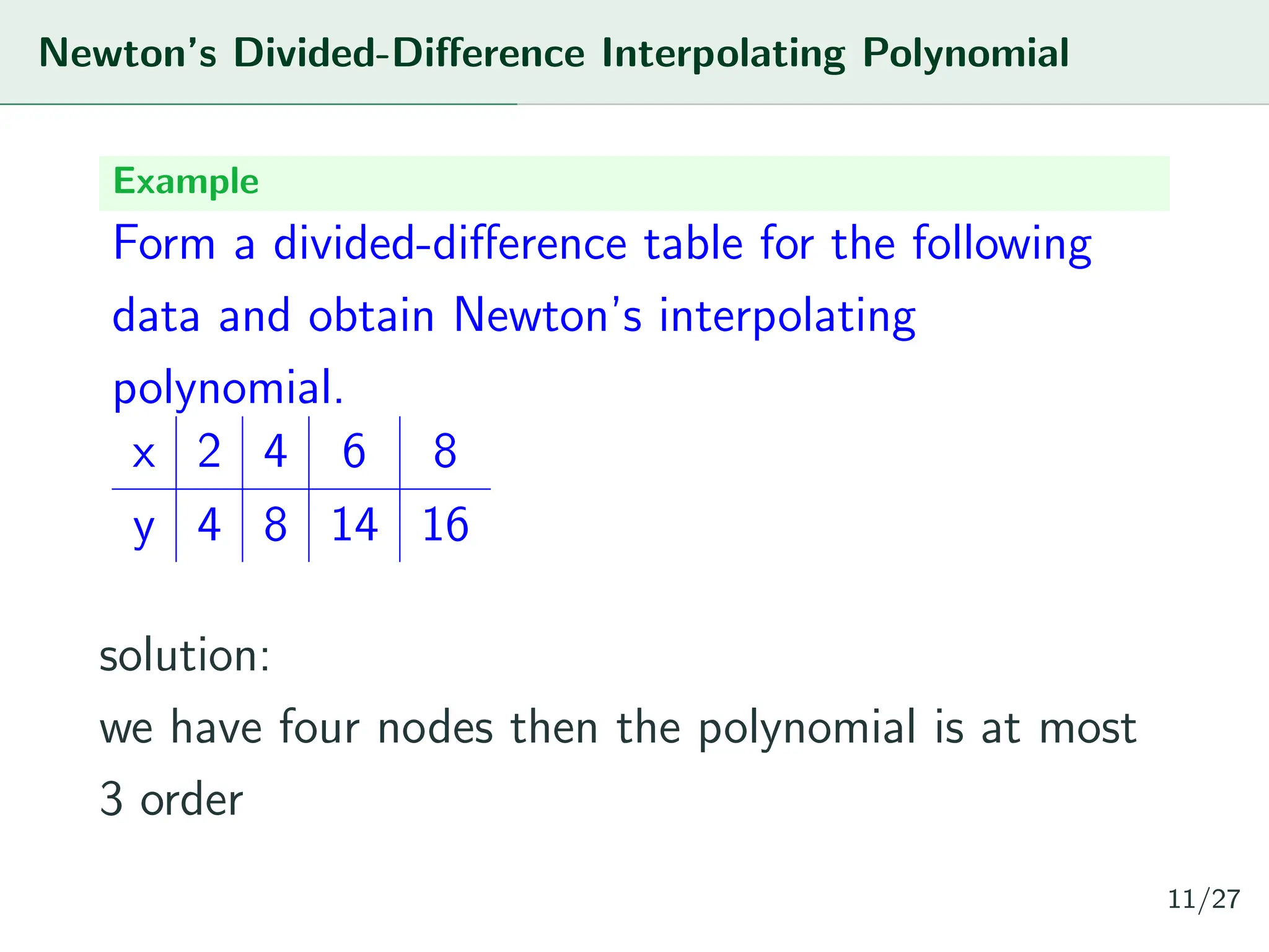
Example
Form a divided-difference table for the following
data and obtain Newton’s interpolating
polynomial.
x 2 4 6 8
y 4 8 14 16
solution:
we have four nodes then the polynomial is at most
3 order
11/27
12.
Newton’s Divided-Difference InterpolatingPolynomial
P3(x) = f [x0] + f [x0, x1](x − x0) + f [x0, x1, x2](x − x0)(x − x1)
+f [x0, x1, x2, x3](x − x0)(x − x1)(x − x2)
Now form the divided difference table by solving
each divided difference.
12/27
Lagrange Interpolating Polynomial
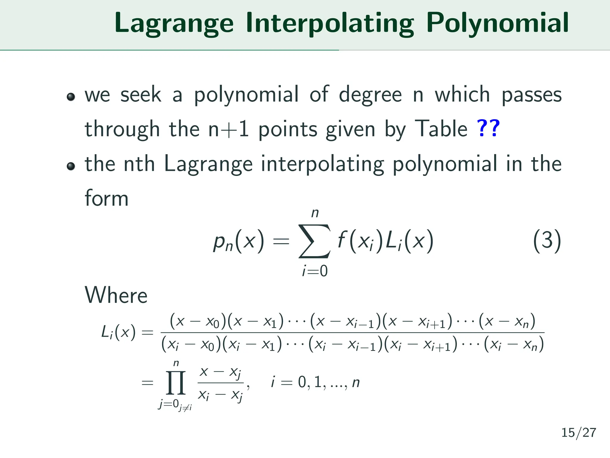
weseek a polynomial of degree n which passes
through the n+1 points given by Table ??
the nth Lagrange interpolating polynomial in the
form
pn(x) =
n
X
i=0
f (xi)Li(x) (3)
Where
Li (x) =
(x − x0)(x − x1) · · · (x − xi−1)(x − xi+1) · · · (x − xn)
(xi − x0)(xi − x1) · · · (xi − xi−1)(xi − xi+1) · · · (xi − xn)
=
n
Y
j=0j̸=i
x − xj
xi − xj
, i = 0, 1, ..., n
15/27
16.
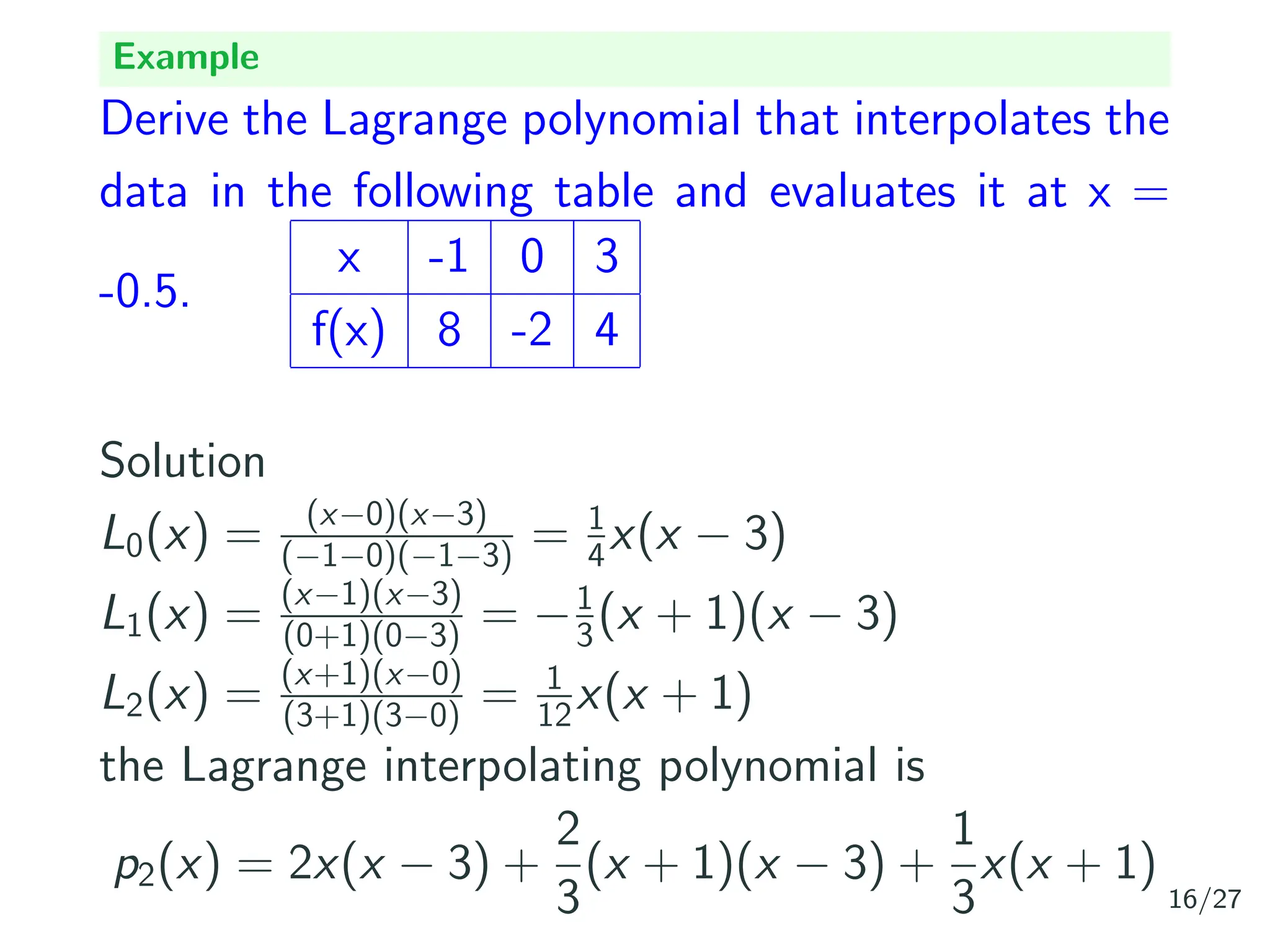
Example
Derive the Lagrangepolynomial that interpolates the
data in the following table and evaluates it at x =
-0.5.
x -1 0 3
f(x) 8 -2 4
Solution
L0(x) = (x−0)(x−3)
(−1−0)(−1−3) = 1
4x(x − 3)
L1(x) = (x−1)(x−3)
(0+1)(0−3) = −1
3(x + 1)(x − 3)
L2(x) = (x+1)(x−0)
(3+1)(3−0) = 1
12x(x + 1)
the Lagrange interpolating polynomial is
p2(x) = 2x(x − 3) +
2
3
(x + 1)(x − 3) +
1
3
x(x + 1)
16/27
17.
Spline interpolation
Many scientificand engineering phenomena being
measured undergo a transition from one physical
domain to another.
Data obtained from these measurements are bet-
ter represented by a set of piecewise continuous
curves rather than by a single curve.
17/27
18.
Let f bea real-valued function defined on some
interval [a, b] and let the set of data points be
given below
x a = x1 x2 · · · xn = b
y f (x1) f (x2) · · · f (xn)
assume that a = x1<x2< · · · <xn = b.
Using the formula of the equation of the line, it
is easy to see that the function S(x) is defined by
Si (x) = f (xi ) +
f (xi+1) − f (xi )
xi+1 − xi
(x − xi )
= f (xi ) + f [xi+1, xi ](x − xi ) for i = 1, 2, ..., n − 1
18/27
19.
Outside the interval[a, b], S(x) is usually defined
by
S(x) =
(
S1(x) if x<a
Sn−1(x) if x>b
Because S(x) is continuous on [a, b], it is called
a spline of degree 1.
Example
Find a first degree spline interpolating the following table:
x 1 2 3 4 5
f(x) 3 4 3 9 1
Use the resulting spline to approximate f(2.3).
19/27
20.
Solution
S1(x) = f(x1) +
f (x2) − f (x1)
x2 − x1
(x − x1) = x + 2
S2(x) = f (x2) +
f (x3) − f (x2)
x3 − x2
(x − x2 = −x + 6
S3(x) = f (x3) +
f (x4) − f (x3)
x4 − x3
(x − x3) = 6x − 16
S4(x) = f (x4) +
f (x5) − f (x4)
x5 − x4
(x − x4) = −8x + 41
S(x) =
x + 2 if x ∈ [1, 2]
−x + 6 if x ∈ [2, 3]
6x − 16 if x ∈ [3, 4]
−8x + 41 if x ∈ [4, 5]
The value x = 2.3 lies in [2, 3] and so f(2.3) ≈ -(2.3) + 6 =
3.7 20/27
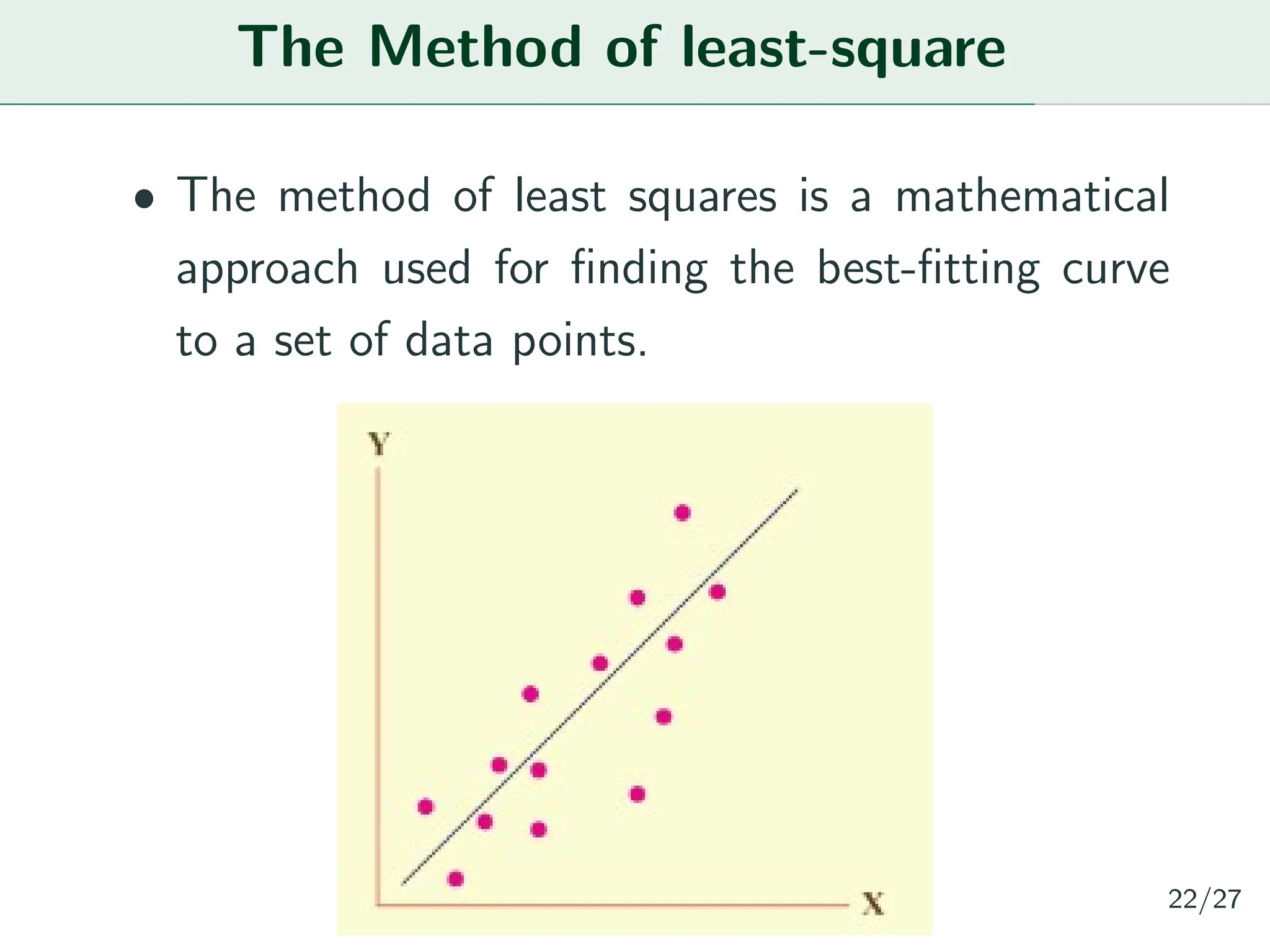
The Method ofleast-square
ˆ The method of least squares is a mathematical
approach used for finding the best-fitting curve
to a set of data points.
22/27
23.
Linear least-square
ˆ Therefore,a reasonable guess function to the data
in Figure 7.2 might be a linear one, that is.
f (x) = ax + b.
ˆ The problem becomes that of finding the values
of the parameters a and b that make f(x) the
“best” function to fit the data.
ˆ The objective of ”least squares” is to minimize
the sum of the squares of the error
23/27
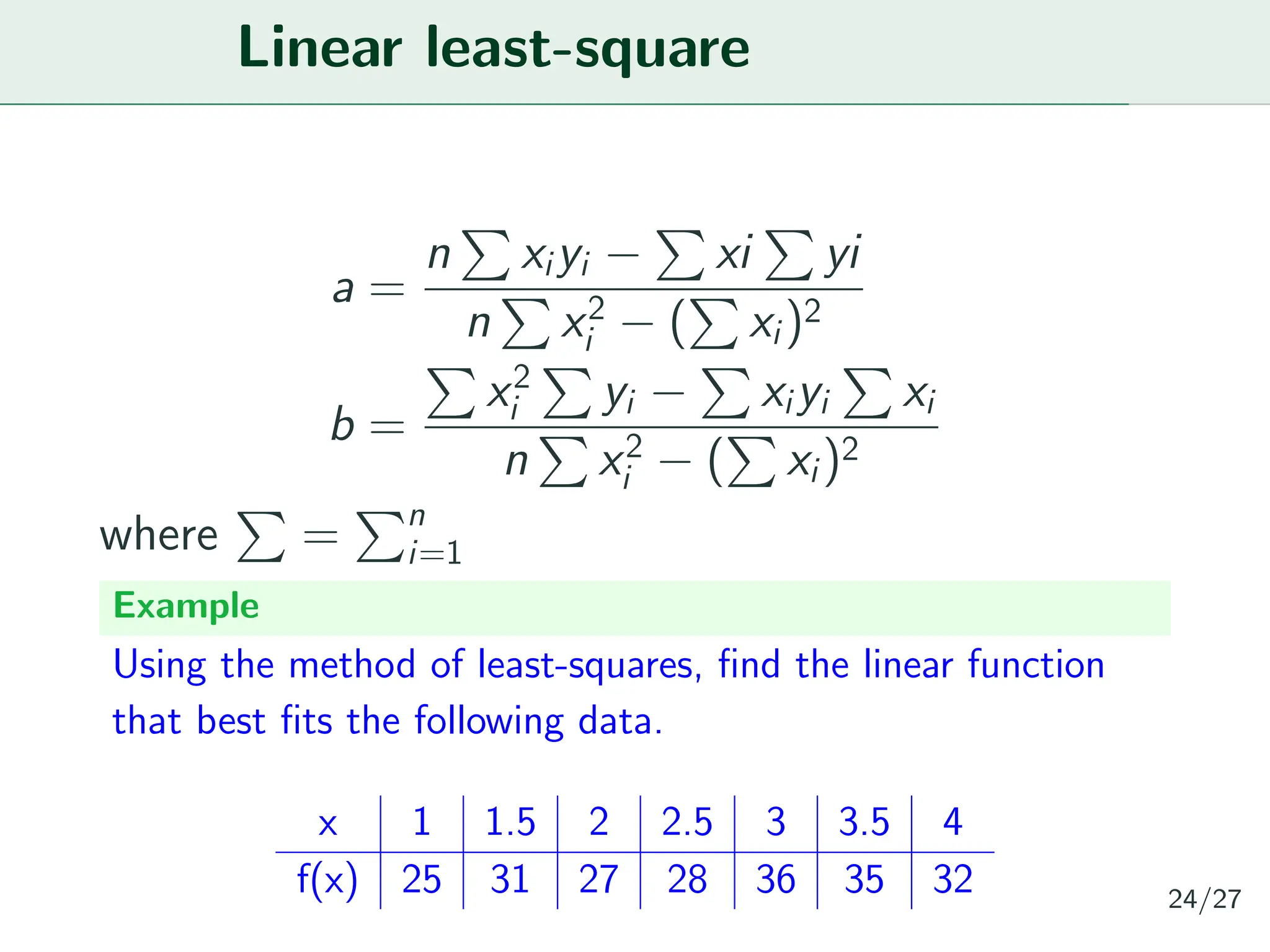
24.
Linear least-square
a =
n
P
xiyi−
P
xi
P
yi
n
P
x2
i − (
P
xi)2
b =
P
x2
i
P
yi −
P
xiyi
P
xi
n
P
x2
i − (
P
xi)2
where
P
=
Pn
i=1
Example
Using the method of least-squares, find the linear function
that best fits the following data.
x 1 1.5 2 2.5 3 3.5 4
f(x) 25 31 27 28 36 35 32 24/27

![Newton’s Divided-Difference Interpolating Polynomial
In this section we want to develop an interpolat-
ing formula that will be more efficient and conve-
nient to use than the one shown in the previous
section
This will avoid the problem of finding the solution
to a system of simultaneous equations.
Pn(x) = f [x0] + f [x0, x1](x − x0)
+f [x0, x1, x2](x − x0)(x − x1)
+ · · · f [x0, x1, x2 · · · , xn](x − x0)(x − x1) · · · (x − xn−1)
7/27](https://image.slidesharecdn.com/chapterfive1-250524062952-4f047c09/75/Computational-methods-for-engineering-7-2048.jpg)
![Newton’s Divided-Difference Interpolating Polynomial
The above equation is know as n-order
newron-divided deference polynomial and where
the notation
f [x0, x1, · · · , xn] =
f [x1, x2, · · · xn] − f [x0, x2, · · · xn−1]
xn − x0
is know as divided-difference
ˆ The first four divided differences denoted as ff
f [x0] = f (x0)
f [x0, x1] =
f [x1] − f [x0]
x1 − x0
8/27](https://image.slidesharecdn.com/chapterfive1-250524062952-4f047c09/75/Computational-methods-for-engineering-8-2048.jpg)
![Newton’s Divided-Difference Interpolating Polynomial
f [x0, x1, x2] =
f [x1, x2] − f [x0, x1]
x2 − x0
f [x0, x1, x2, x3] =
f [x1, x2, x3] − f [x0, x1, x2]
x3 − x0
ˆ The divided difference canbe illustrated best in
table form as shown in table 2
9/27](https://image.slidesharecdn.com/chapterfive1-250524062952-4f047c09/75/Computational-methods-for-engineering-9-2048.jpg)
![Newton’s Divided-Difference Interpolating Polynomial
Table 2: divided differences.
xi f[xi] f[xi,xi+1] f[xi,xi+1,xi+2] · · ·
x0 f[x0]
f[x0,x1]
x1 f[x1] f[x0,x1,x2]
f[x1,x2] · · ·
x2 f[x2] f[x1,x2,x3]
f[x2,x3] · · ·
x3 f[x3] f[x2,x3,x4]
f[x3,x4] 10/27](https://image.slidesharecdn.com/chapterfive1-250524062952-4f047c09/75/Computational-methods-for-engineering-10-2048.jpg)
![Newton’s Divided-Difference Interpolating Polynomial
P3(x) = f [x0] + f [x0, x1](x − x0) + f [x0, x1, x2](x − x0)(x − x1)
+f [x0, x1, x2, x3](x − x0)(x − x1)(x − x2)
Now form the divided difference table by solving
each divided difference.
12/27](https://image.slidesharecdn.com/chapterfive1-250524062952-4f047c09/75/Computational-methods-for-engineering-12-2048.jpg)
![Newton’s Divided-Difference Interpolating Polynomial
xi f[xi] f[xi,xi+1] f[xi,xi+1,xi+2] f[xi,xi+1,xi+2,xi+3]
2 4
2
4 8 0.25
3 -0.125
6 14 -0.5
1
8 16
13/27](https://image.slidesharecdn.com/chapterfive1-250524062952-4f047c09/75/Computational-methods-for-engineering-13-2048.jpg)
![Let f be a real-valued function defined on some
interval [a, b] and let the set of data points be
given below
x a = x1 x2 · · · xn = b
y f (x1) f (x2) · · · f (xn)
assume that a = x1<x2< · · · <xn = b.
Using the formula of the equation of the line, it
is easy to see that the function S(x) is defined by
Si (x) = f (xi ) +
f (xi+1) − f (xi )
xi+1 − xi
(x − xi )
= f (xi ) + f [xi+1, xi ](x − xi ) for i = 1, 2, ..., n − 1
18/27](https://image.slidesharecdn.com/chapterfive1-250524062952-4f047c09/75/Computational-methods-for-engineering-18-2048.jpg)
![Outside the interval [a, b], S(x) is usually defined
by
S(x) =
(
S1(x) if x<a
Sn−1(x) if x>b
Because S(x) is continuous on [a, b], it is called
a spline of degree 1.
Example
Find a first degree spline interpolating the following table:
x 1 2 3 4 5
f(x) 3 4 3 9 1
Use the resulting spline to approximate f(2.3).
19/27](https://image.slidesharecdn.com/chapterfive1-250524062952-4f047c09/75/Computational-methods-for-engineering-19-2048.jpg)
![Solution
S1(x) = f (x1) +
f (x2) − f (x1)
x2 − x1
(x − x1) = x + 2
S2(x) = f (x2) +
f (x3) − f (x2)
x3 − x2
(x − x2 = −x + 6
S3(x) = f (x3) +
f (x4) − f (x3)
x4 − x3
(x − x3) = 6x − 16
S4(x) = f (x4) +
f (x5) − f (x4)
x5 − x4
(x − x4) = −8x + 41
S(x) =
x + 2 if x ∈ [1, 2]
−x + 6 if x ∈ [2, 3]
6x − 16 if x ∈ [3, 4]
−8x + 41 if x ∈ [4, 5]
The value x = 2.3 lies in [2, 3] and so f(2.3) ≈ -(2.3) + 6 =
3.7 20/27](https://image.slidesharecdn.com/chapterfive1-250524062952-4f047c09/75/Computational-methods-for-engineering-20-2048.jpg)


![Newton’s Divided-Difference Interpolating Polynomial
In this section we want to develop an interpolat-
ing formula that will be more efficient and conve-
nient to use than the one shown in the previous
section
This will avoid the problem of finding the solution
to a system of simultaneous equations.
Pn(x) = f [x0] + f [x0, x1](x − x0)
+f [x0, x1, x2](x − x0)(x − x1)
+ · · · f [x0, x1, x2 · · · , xn](x − x0)(x − x1) · · · (x − xn−1)
7/27](https://crownmelresort.com/image.slidesharecdn.com/chapterfive1-250524062952-4f047c09/75/Computational-methods-for-engineering-7-2048.jpg)
![Newton’s Divided-Difference Interpolating Polynomial
The above equation is know as n-order
newron-divided deference polynomial and where
the notation
f [x0, x1, · · · , xn] =
f [x1, x2, · · · xn] − f [x0, x2, · · · xn−1]
xn − x0
is know as divided-difference
ˆ The first four divided differences denoted as ff
f [x0] = f (x0)
f [x0, x1] =
f [x1] − f [x0]
x1 − x0
8/27](https://crownmelresort.com/image.slidesharecdn.com/chapterfive1-250524062952-4f047c09/75/Computational-methods-for-engineering-8-2048.jpg)
![Newton’s Divided-Difference Interpolating Polynomial
f [x0, x1, x2] =
f [x1, x2] − f [x0, x1]
x2 − x0
f [x0, x1, x2, x3] =
f [x1, x2, x3] − f [x0, x1, x2]
x3 − x0
ˆ The divided difference canbe illustrated best in
table form as shown in table 2
9/27](https://crownmelresort.com/image.slidesharecdn.com/chapterfive1-250524062952-4f047c09/75/Computational-methods-for-engineering-9-2048.jpg)
![Newton’s Divided-Difference Interpolating Polynomial
Table 2: divided differences.
xi f[xi] f[xi,xi+1] f[xi,xi+1,xi+2] · · ·
x0 f[x0]
f[x0,x1]
x1 f[x1] f[x0,x1,x2]
f[x1,x2] · · ·
x2 f[x2] f[x1,x2,x3]
f[x2,x3] · · ·
x3 f[x3] f[x2,x3,x4]
f[x3,x4] 10/27](https://crownmelresort.com/image.slidesharecdn.com/chapterfive1-250524062952-4f047c09/75/Computational-methods-for-engineering-10-2048.jpg)

![Newton’s Divided-Difference Interpolating Polynomial
P3(x) = f [x0] + f [x0, x1](x − x0) + f [x0, x1, x2](x − x0)(x − x1)
+f [x0, x1, x2, x3](x − x0)(x − x1)(x − x2)
Now form the divided difference table by solving
each divided difference.
12/27](https://crownmelresort.com/image.slidesharecdn.com/chapterfive1-250524062952-4f047c09/75/Computational-methods-for-engineering-12-2048.jpg)
![Newton’s Divided-Difference Interpolating Polynomial
xi f[xi] f[xi,xi+1] f[xi,xi+1,xi+2] f[xi,xi+1,xi+2,xi+3]
2 4
2
4 8 0.25
3 -0.125
6 14 -0.5
1
8 16
13/27](https://crownmelresort.com/image.slidesharecdn.com/chapterfive1-250524062952-4f047c09/75/Computational-methods-for-engineering-13-2048.jpg)


![Let f be a real-valued function defined on some
interval [a, b] and let the set of data points be
given below
x a = x1 x2 · · · xn = b
y f (x1) f (x2) · · · f (xn)
assume that a = x1<x2< · · · <xn = b.
Using the formula of the equation of the line, it
is easy to see that the function S(x) is defined by
Si (x) = f (xi ) +
f (xi+1) − f (xi )
xi+1 − xi
(x − xi )
= f (xi ) + f [xi+1, xi ](x − xi ) for i = 1, 2, ..., n − 1
18/27](https://crownmelresort.com/image.slidesharecdn.com/chapterfive1-250524062952-4f047c09/75/Computational-methods-for-engineering-18-2048.jpg)
![Outside the interval [a, b], S(x) is usually defined
by
S(x) =
(
S1(x) if x<a
Sn−1(x) if x>b
Because S(x) is continuous on [a, b], it is called
a spline of degree 1.
Example
Find a first degree spline interpolating the following table:
x 1 2 3 4 5
f(x) 3 4 3 9 1
Use the resulting spline to approximate f(2.3).
19/27](https://crownmelresort.com/image.slidesharecdn.com/chapterfive1-250524062952-4f047c09/75/Computational-methods-for-engineering-19-2048.jpg)
![Solution
S1(x) = f (x1) +
f (x2) − f (x1)
x2 − x1
(x − x1) = x + 2
S2(x) = f (x2) +
f (x3) − f (x2)
x3 − x2
(x − x2 = −x + 6
S3(x) = f (x3) +
f (x4) − f (x3)
x4 − x3
(x − x3) = 6x − 16
S4(x) = f (x4) +
f (x5) − f (x4)
x5 − x4
(x − x4) = −8x + 41
S(x) =
x + 2 if x ∈ [1, 2]
−x + 6 if x ∈ [2, 3]
6x − 16 if x ∈ [3, 4]
−8x + 41 if x ∈ [4, 5]
The value x = 2.3 lies in [2, 3] and so f(2.3) ≈ -(2.3) + 6 =
3.7 20/27](https://crownmelresort.com/image.slidesharecdn.com/chapterfive1-250524062952-4f047c09/75/Computational-methods-for-engineering-20-2048.jpg)


![ANPARA THERMAL POWER STATION[1] sangam.pdf](https://cdn.slidesharecdn.com/ss_thumbnails/anparathermalpowerstation1sangam-251121115219-9261cde4-thumbnail.jpg?width=640&height=640&fit=bounds)


