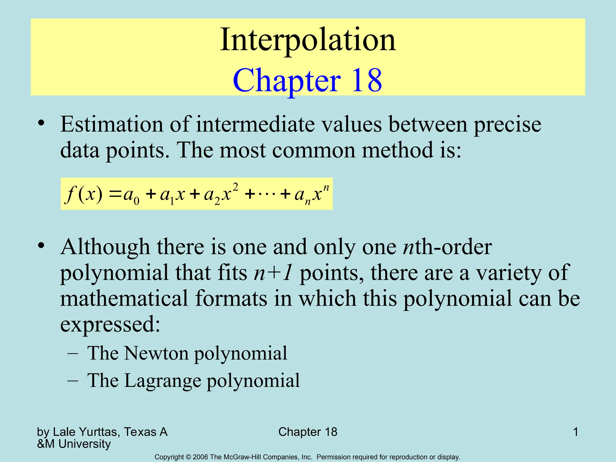
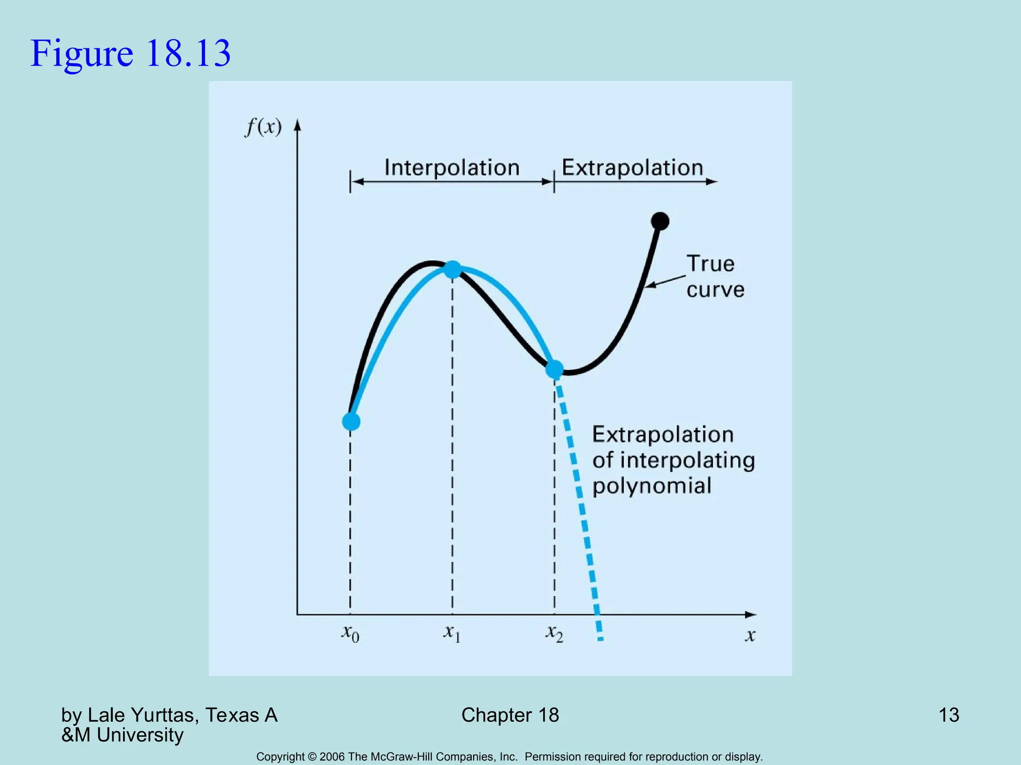
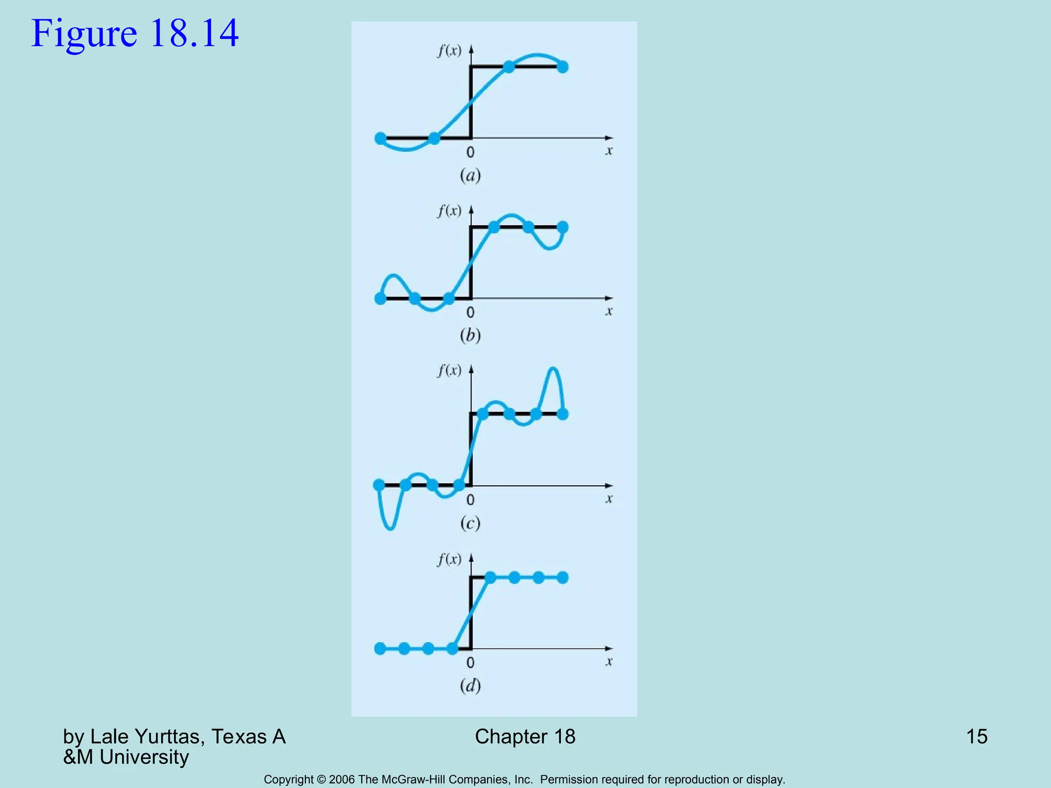
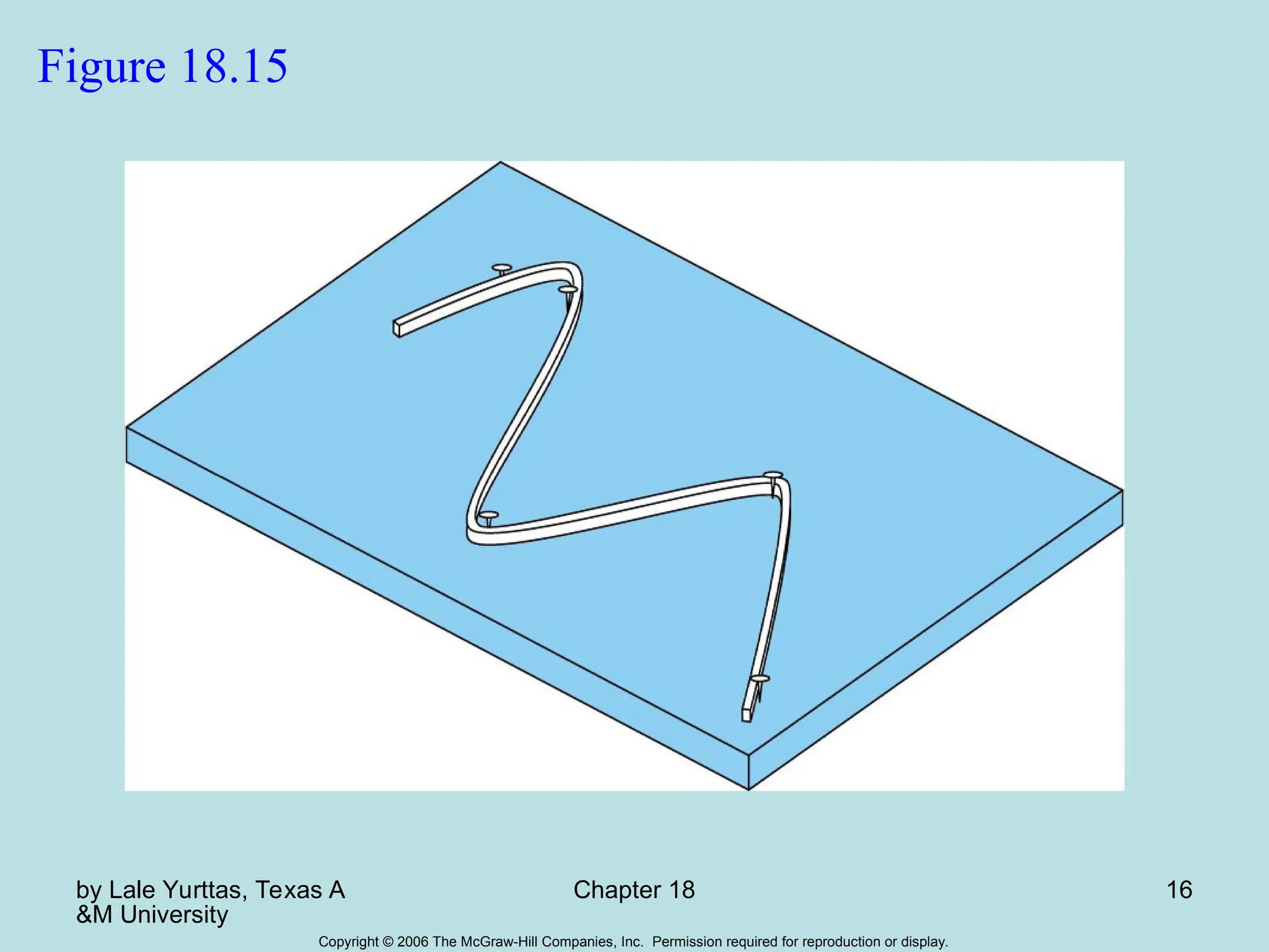
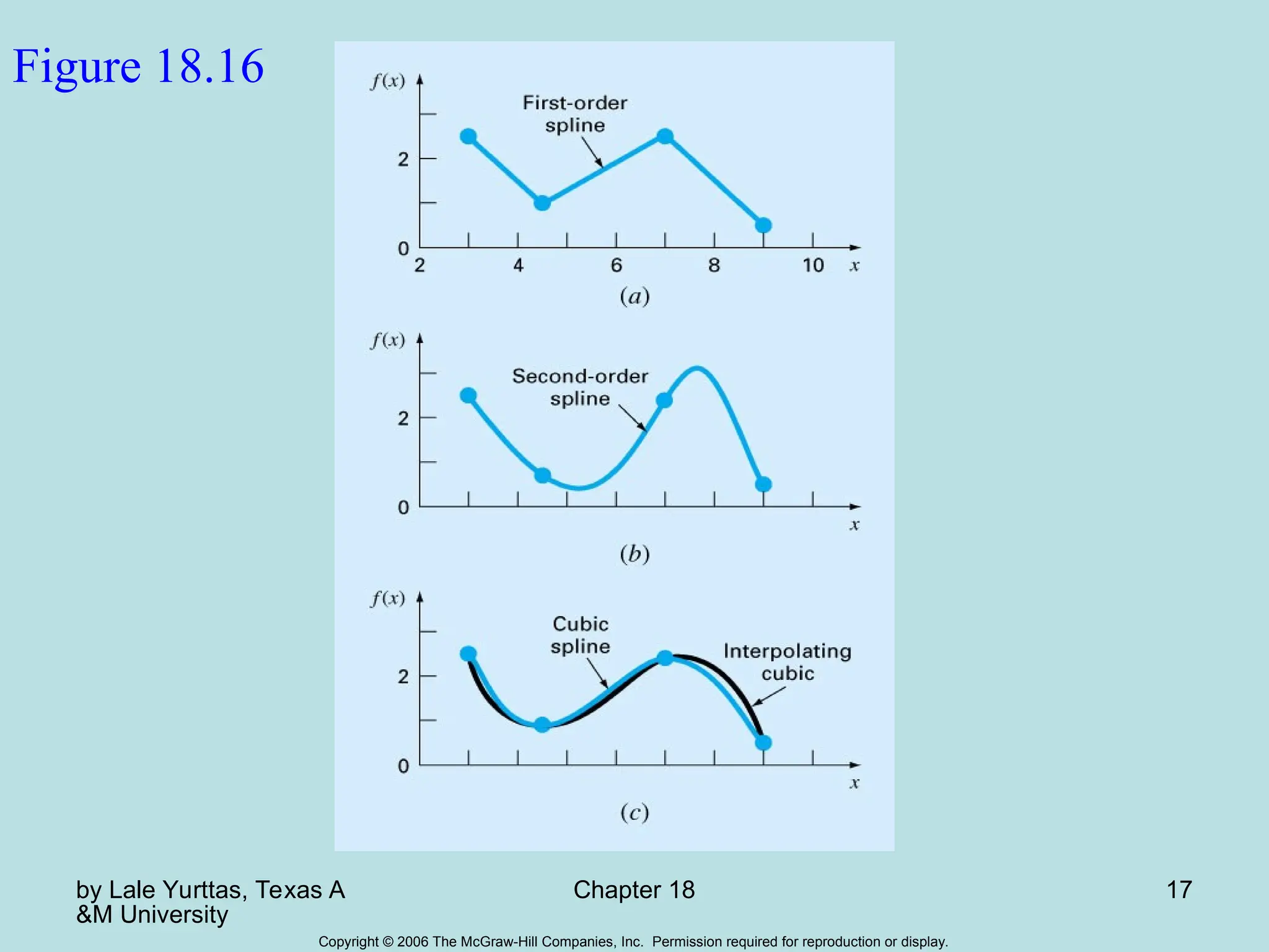
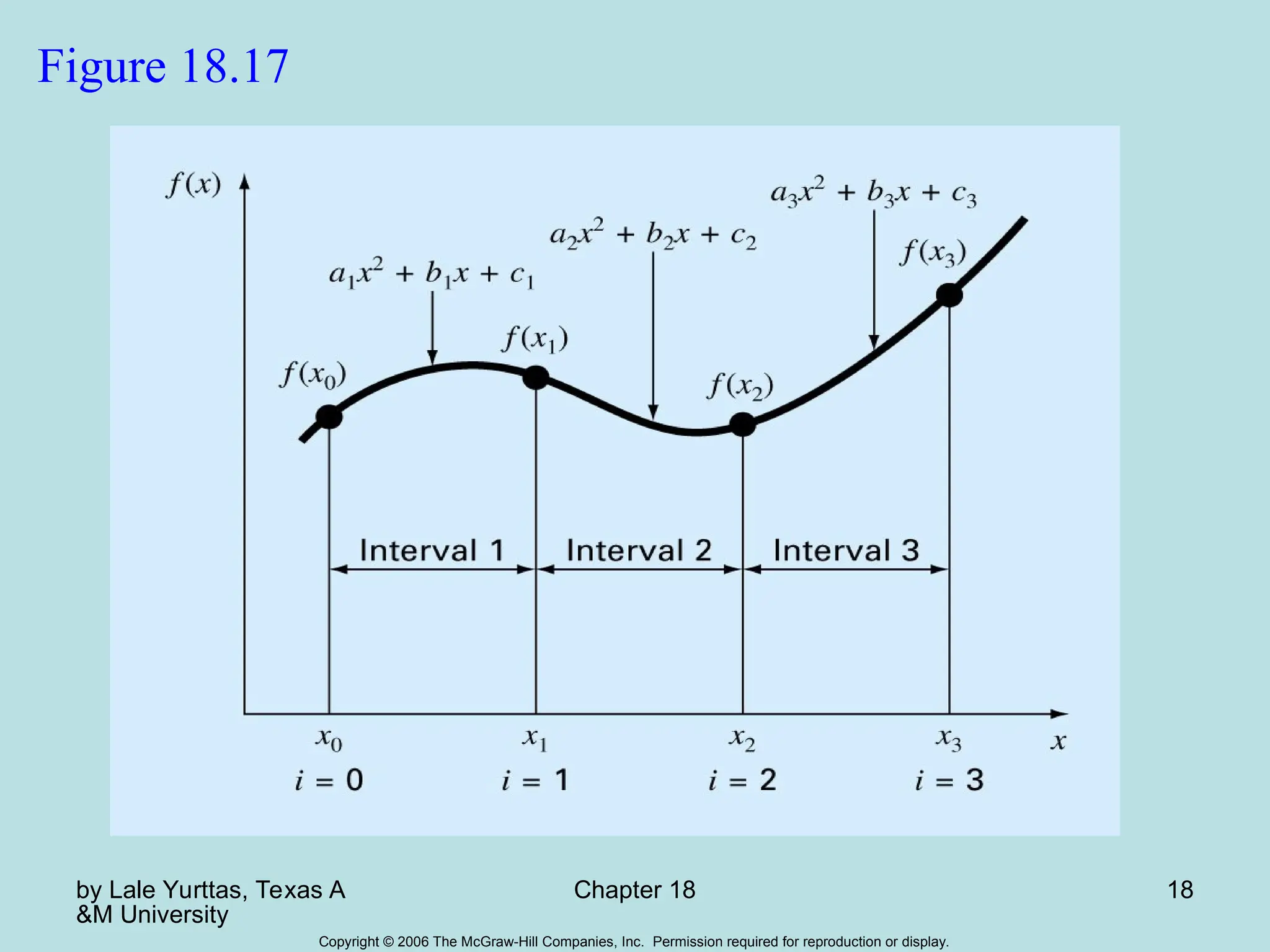
Chapter 18 discusses interpolation methods for estimating values between data points, primarily focusing on Newton's and Lagrange's polynomials. Newton's method includes polynomial forms and error analysis, while Lagrange's reformulates the polynomial to avoid divided differences. Additionally, the chapter introduces spline interpolation as an alternative to polynomials to mitigate issues with round-off error and overshoot.
![by Lale Yurttas, Texas A
&M University
Chapter 18 6
Copyright © 2006 The McGraw-Hill Companies, Inc. Permission required for reproduction or display.
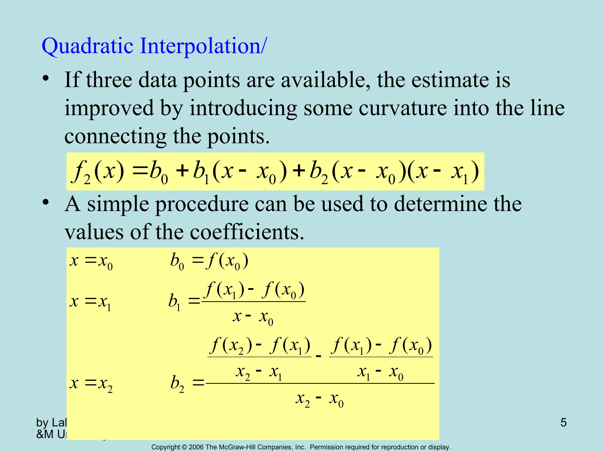
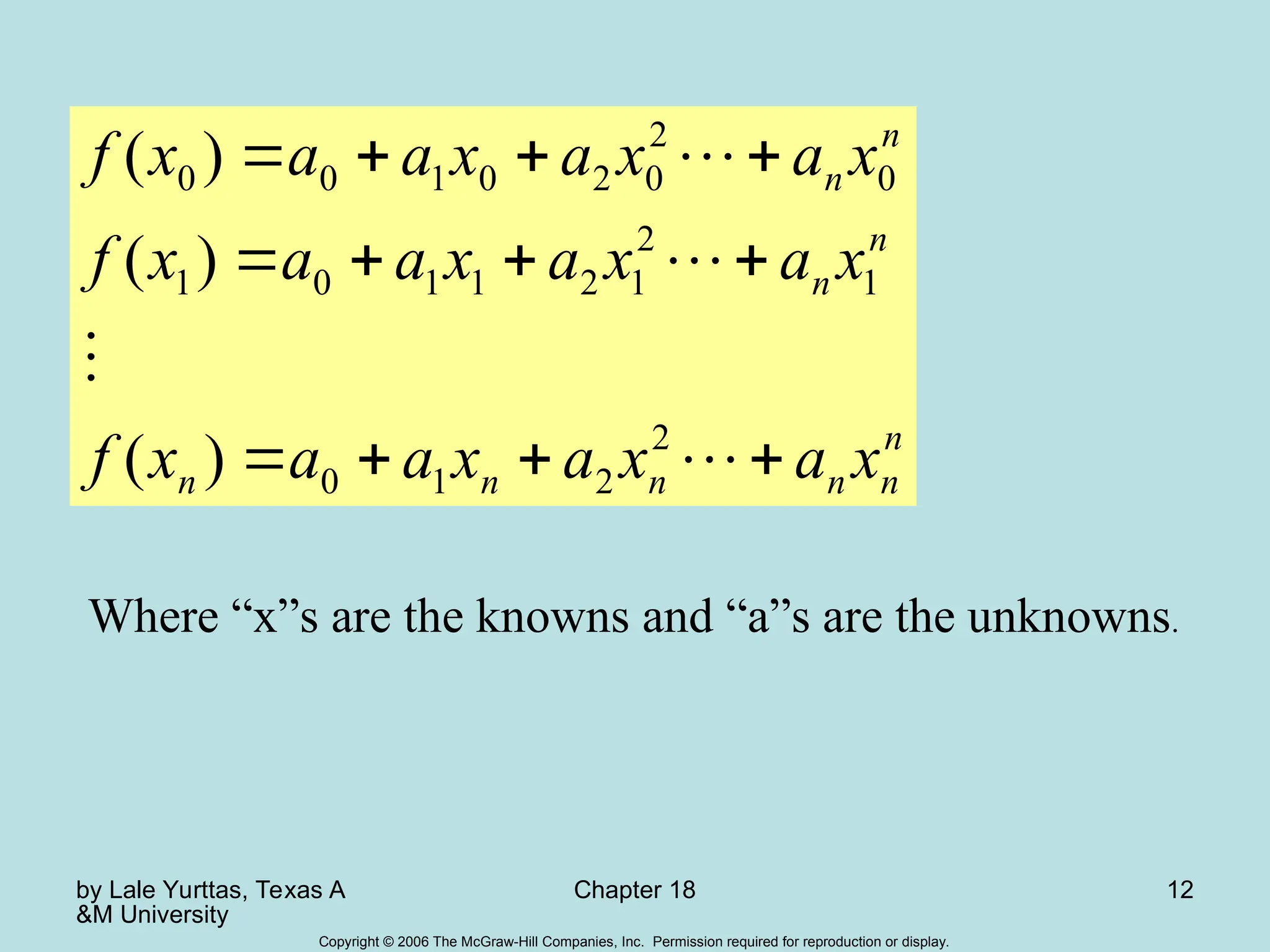
General Form of Newton’s Interpolating Polynomials/
0
0
2
1
1
1
0
1
1
0
1
1
0
1
2
2
0
1
1
0
0
0
1
1
1
0
0
1
2
1
0
0
1
0
0
]
,
,
,
[
]
,
,
,
[
]
,
,
,
,
[
]
,
[
]
,
[
]
,
,
[
)
(
)
(
]
,
[
]
,
,
,
,
[
]
,
,
[
]
,
[
)
(
]
,
,
,
[
)
(
)
)(
(
]
,
,
[
)
)(
(
]
,
[
)
(
)
(
)
(
x
x
x
x
x
f
x
x
x
f
x
x
x
x
f
x
x
x
x
f
x
x
f
x
x
x
f
x
x
x
f
x
f
x
x
f
x
x
x
x
f
b
x
x
x
f
b
x
x
f
b
x
f
b
x
x
x
f
x
x
x
x
x
x
x
x
x
f
x
x
x
x
x
x
f
x
x
x
f
x
f
n
n
n
n
n
n
n
k
i
k
j
j
i
k
j
i
j
i
j
i
j
i
n
n
n
n
n
n
n
Bracketed function
evaluations are finite
divided differences](https://image.slidesharecdn.com/chap18-250122111444-b3d9187a/75/Chap_18-ppt-on-interpolation-basics-undersatanding-6-2048.jpg)

![by Lale Yurttas, Texas A
&M University
Chapter 18 9
Copyright © 2006 The McGraw-Hill Companies, Inc. Permission required for reproduction or display.
)
(
)
(
)
(
)
(
)
(
)
(
)
(
2
1
2
0
2
1
0
1
2
1
0
1
2
0
0
2
0
1
0
2
1
2
1
0
1
0
0
1
0
1
1
x
f
x
x
x
x
x
x
x
x
x
f
x
x
x
x
x
x
x
x
x
f
x
x
x
x
x
x
x
x
x
f
x
f
x
x
x
x
x
f
x
x
x
x
x
f
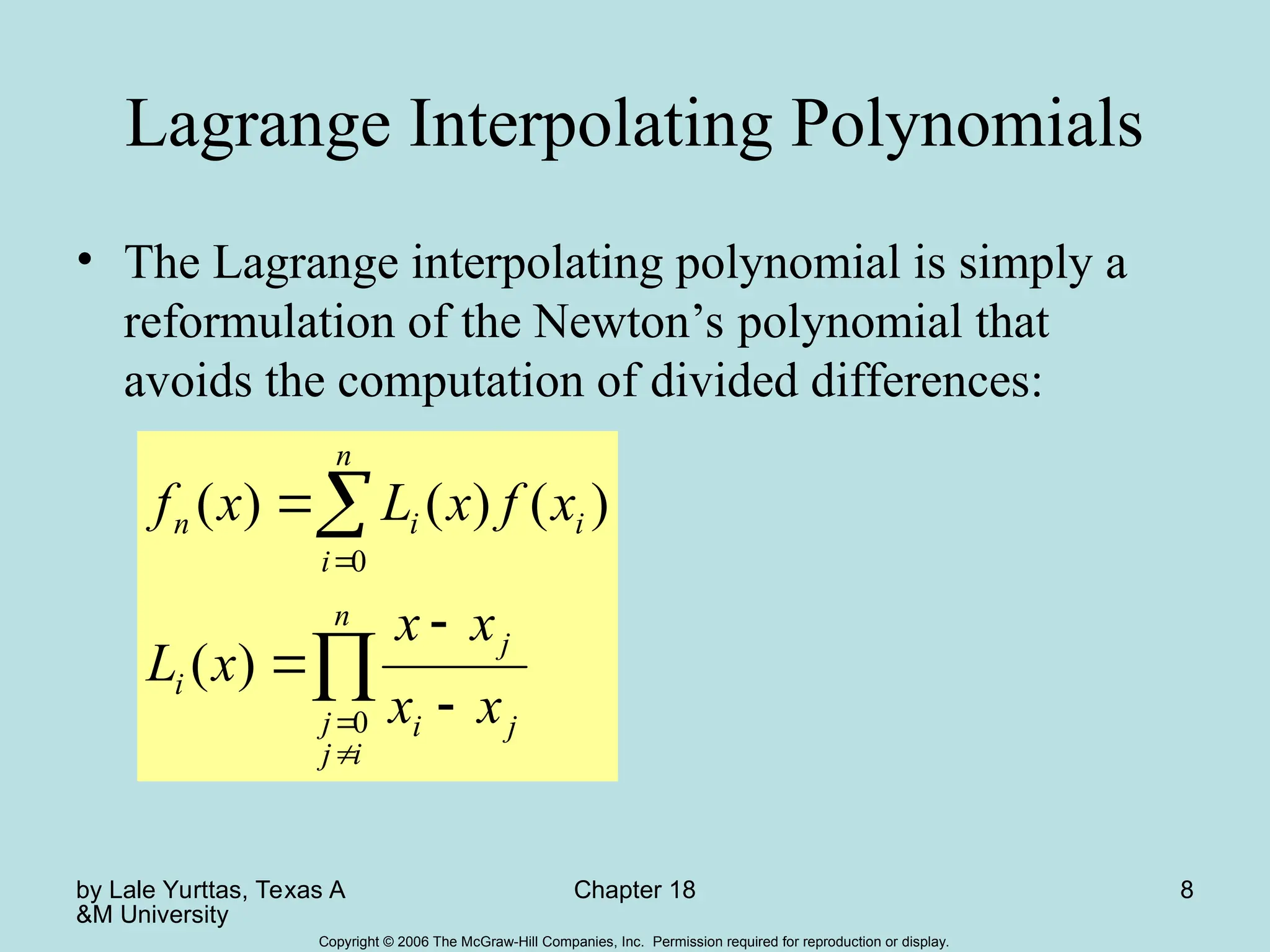
•As with Newton’s method, the Lagrange version has an
estimated error of:
n
i
i
n
n
n x
x
x
x
x
x
f
R
0
0
1 )
(
]
,
,
,
,
[ ](https://image.slidesharecdn.com/chap18-250122111444-b3d9187a/75/Chap_18-ppt-on-interpolation-basics-undersatanding-9-2048.jpg)


![by Lale Yurttas, Texas A
&M University
Chapter 18 6
Copyright © 2006 The McGraw-Hill Companies, Inc. Permission required for reproduction or display.
General Form of Newton’s Interpolating Polynomials/
0
0
2
1
1
1
0
1
1
0
1
1
0
1
2
2
0
1
1
0
0
0
1
1
1
0
0
1
2
1
0
0
1
0
0
]
,
,
,
[
]
,
,
,
[
]
,
,
,
,
[
]
,
[
]
,
[
]
,
,
[
)
(
)
(
]
,
[
]
,
,
,
,
[
]
,
,
[
]
,
[
)
(
]
,
,
,
[
)
(
)
)(
(
]
,
,
[
)
)(
(
]
,
[
)
(
)
(
)
(
x
x
x
x
x
f
x
x
x
f
x
x
x
x
f
x
x
x
x
f
x
x
f
x
x
x
f
x
x
x
f
x
f
x
x
f
x
x
x
x
f
b
x
x
x
f
b
x
x
f
b
x
f
b
x
x
x
f
x
x
x
x
x
x
x
x
x
f
x
x
x
x
x
x
f
x
x
x
f
x
f
n
n
n
n
n
n
n
k
i
k
j
j
i
k
j
i
j
i
j
i
j
i
n
n
n
n
n
n
n
Bracketed function
evaluations are finite
divided differences](https://crownmelresort.com/image.slidesharecdn.com/chap18-250122111444-b3d9187a/75/Chap_18-ppt-on-interpolation-basics-undersatanding-6-2048.jpg)


![by Lale Yurttas, Texas A
&M University
Chapter 18 9
Copyright © 2006 The McGraw-Hill Companies, Inc. Permission required for reproduction or display.
)
(
)
(
)
(
)
(
)
(
)
(
)
(
2
1
2
0
2
1
0
1
2
1
0
1
2
0
0
2
0
1
0
2
1
2
1
0
1
0
0
1
0
1
1
x
f
x
x
x
x
x
x
x
x
x
f
x
x
x
x
x
x
x
x
x
f
x
x
x
x
x
x
x
x
x
f
x
f
x
x
x
x
x
f
x
x
x
x
x
f
•As with Newton’s method, the Lagrange version has an
estimated error of:
n
i
i
n
n
n x
x
x
x
x
x
f
R
0
0
1 )
(
]
,
,
,
,
[ ](https://crownmelresort.com/image.slidesharecdn.com/chap18-250122111444-b3d9187a/75/Chap_18-ppt-on-interpolation-basics-undersatanding-9-2048.jpg)


![ANPARA THERMAL POWER STATION[1] sangam.pdf](https://cdn.slidesharecdn.com/ss_thumbnails/anparathermalpowerstation1sangam-251121115219-9261cde4-thumbnail.jpg?width=640&height=640&fit=bounds)


