Download to read offline

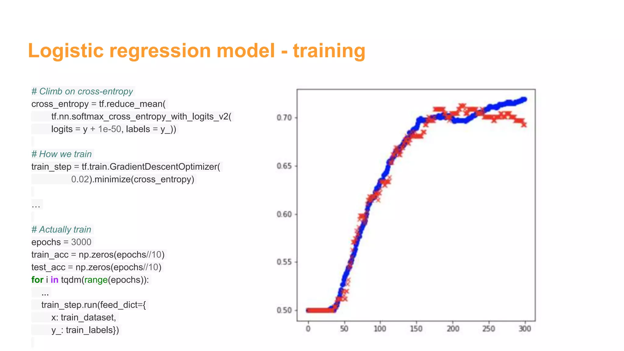
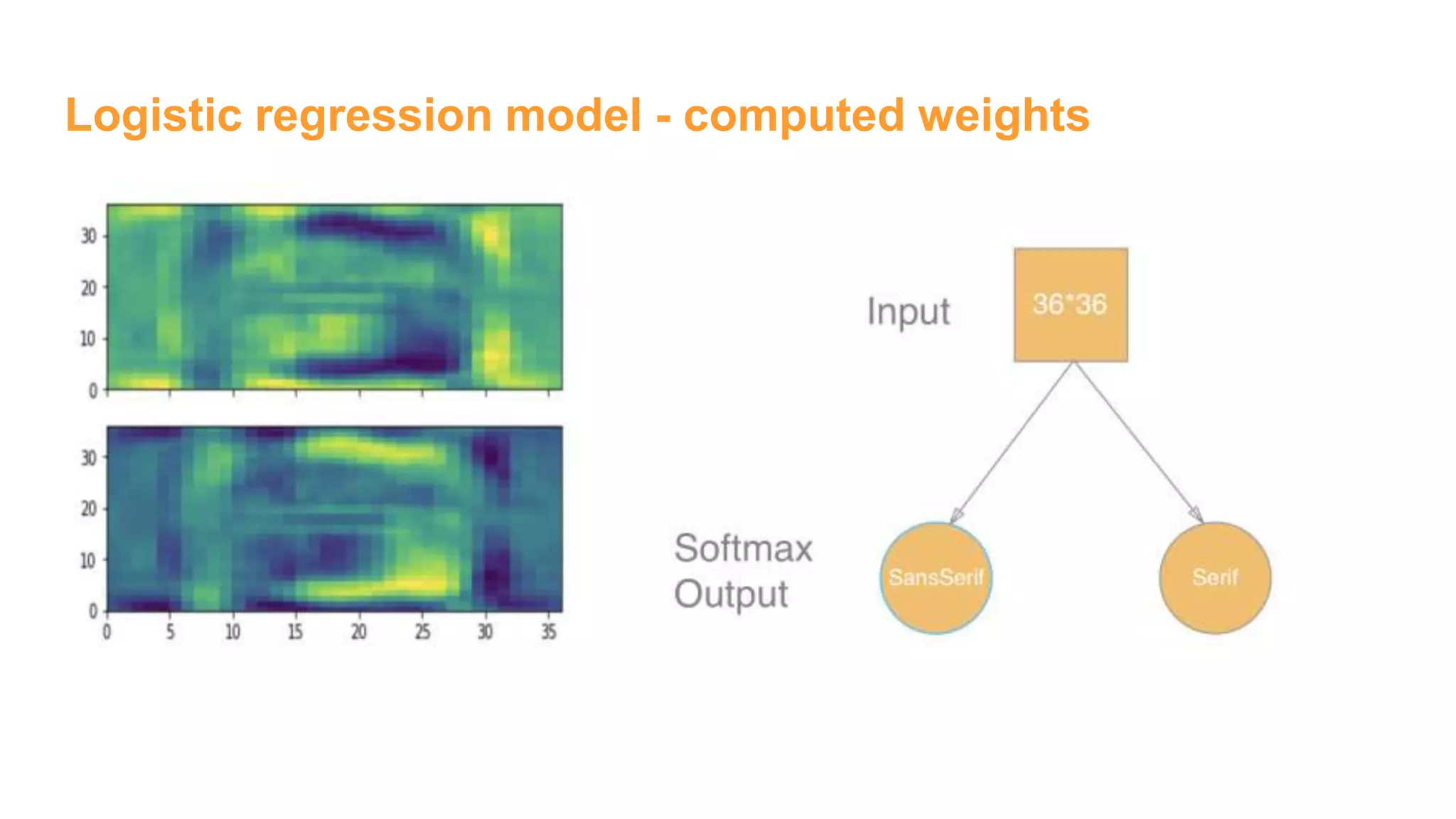
![Logistic regression model - build model
sess = tf.InteractiveSession()
# These will be inputs
## Input pixels, flattened
x = tf.placeholder("float", [None, 1296])
## Known labels
y_ = tf.placeholder("float", [None,2])
# Variables
W = tf.Variable(tf.zeros([1296,2]))
b = tf.Variable(tf.zeros([2]))
# Just initialize
sess.run(tf.global_variables_initializer())
# Define model
y = tf.nn.softmax(tf.matmul(x,W) + b)
### End model specification, begin training code](https://image.slidesharecdn.com/womeninai-fontclassificationwith5deeplearningmodelsusingtensorflow-190331022227/75/Font-classification-with-5-deep-learning-models-using-tensor-flow-7-2048.jpg)
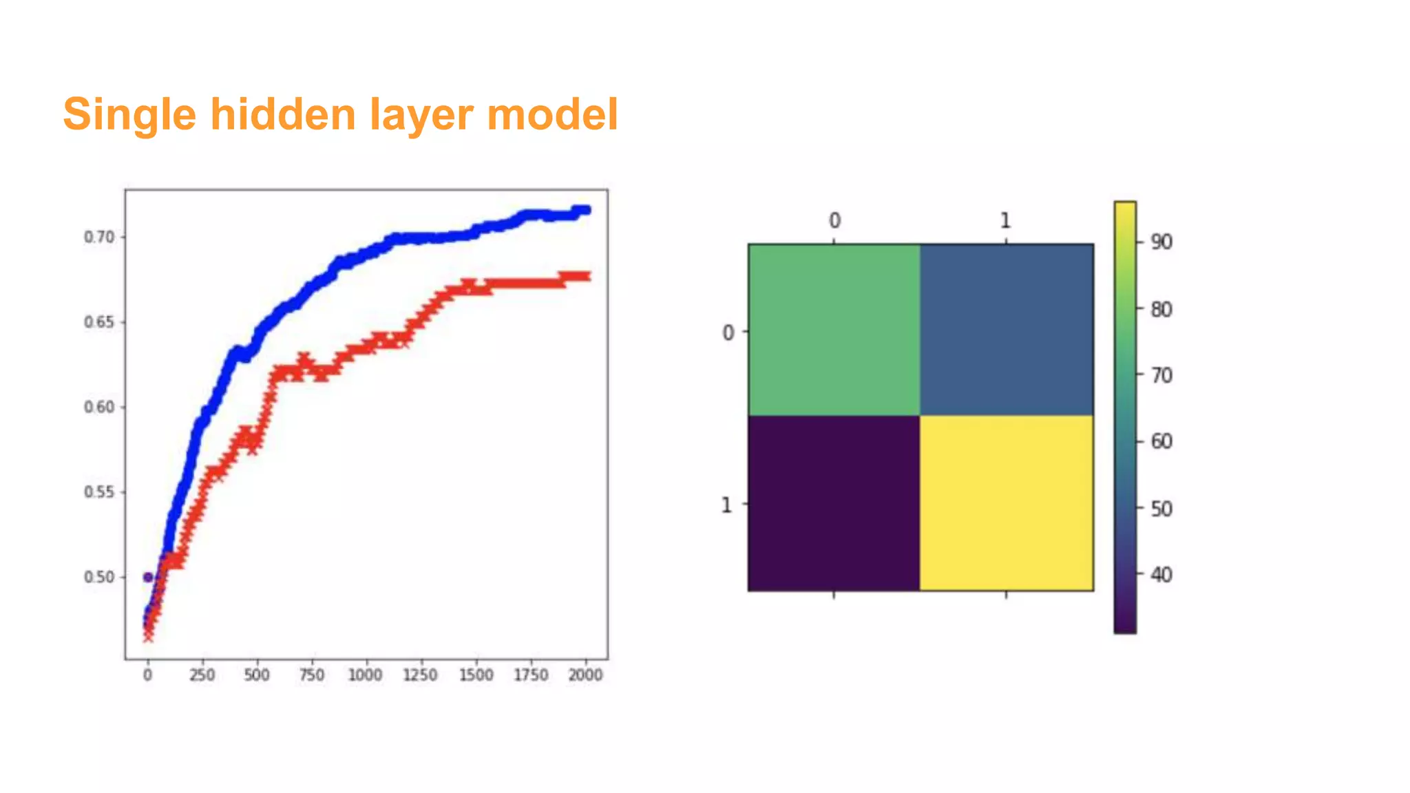
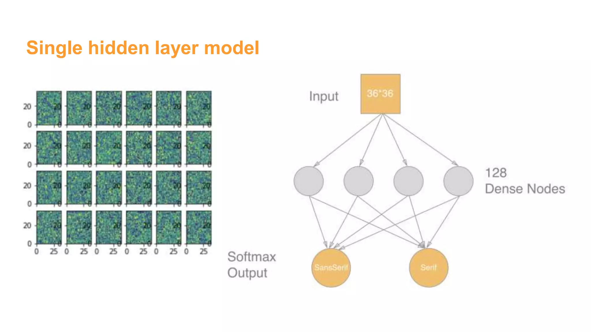
![Single hidden layer model
# Hidden layer
num_hidden = 128
W1 = tf.Variable(tf.truncated_normal([1296, num_hidden],
stddev=1./math.sqrt(1296)))
b1 = tf.Variable(tf.constant(0.1,shape=[num_hidden]))
h1 = tf.sigmoid(tf.matmul(x,W1) + b1)
# Output Layer
W2 = tf.Variable(tf.truncated_normal([num_hidden, 2],
stddev=1./math.sqrt(2)))
b2 = tf.Variable(tf.constant(0.1,shape=[2]))
# Just initialize
sess.run(tf.global_variables_initializer())
# Define model
y = tf.nn.softmax(tf.matmul(h1,W2) + b2)
### End model specification, begin training code
# Actually train
epochs = 20000
train_acc = np.zeros(epochs//10)
test_acc = np.zeros(epochs//10)
for i in tqdm(range(epochs), ascii=True):
if i % 10 == 0:
# Check accuracy on train set
A = accuracy.eval(feed_dict={
x: train_dataset,
y_: train_labels})
train_acc[i//10] = A
# And now the validation set
A = accuracy.eval(feed_dict={
x: valid_dataset,
y_: valid_labels})
test_acc[i//10] = A
train_step.run(feed_dict={
x: train_dataset,
y_: train_labels})](https://image.slidesharecdn.com/womeninai-fontclassificationwith5deeplearningmodelsusingtensorflow-190331022227/75/Font-classification-with-5-deep-learning-models-using-tensor-flow-10-2048.jpg)
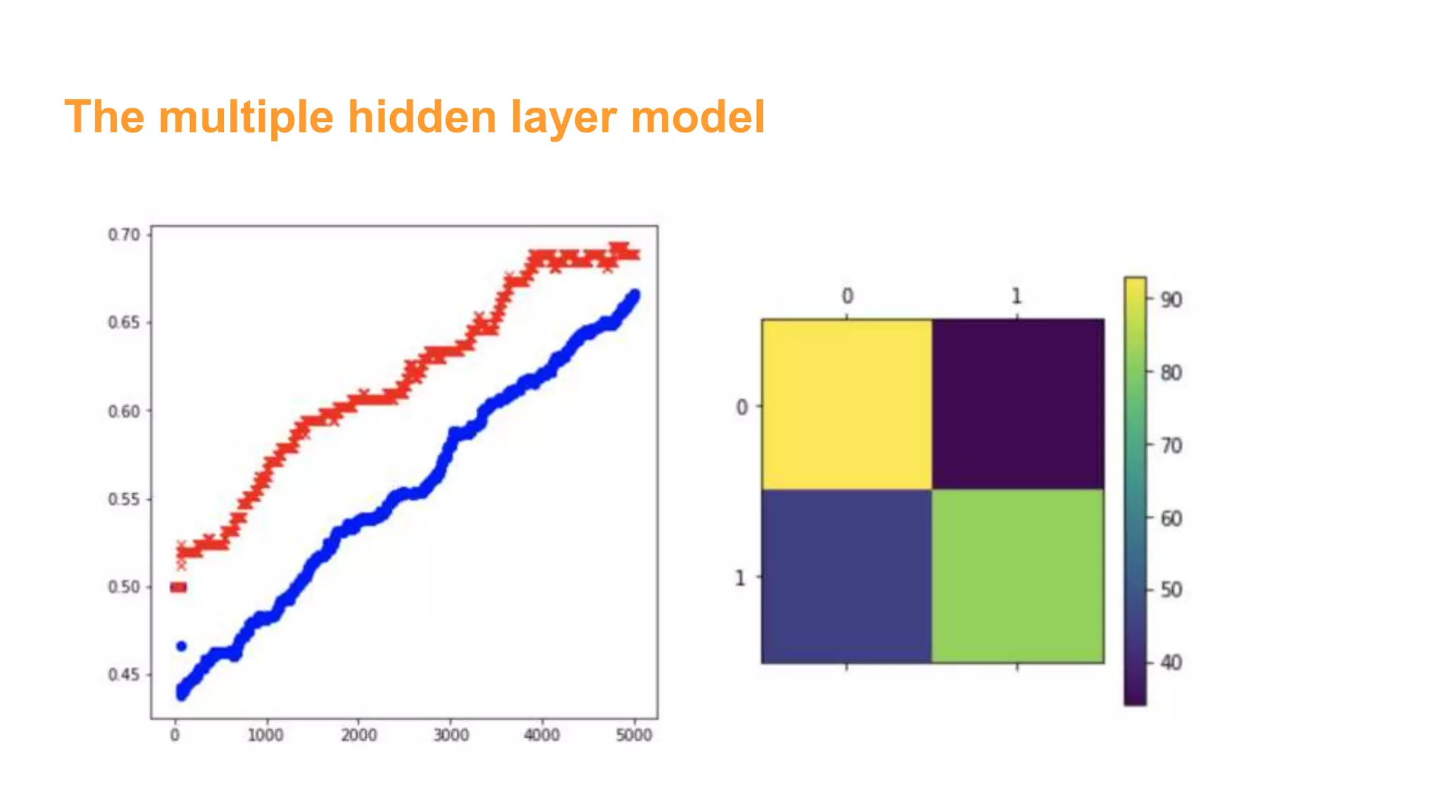
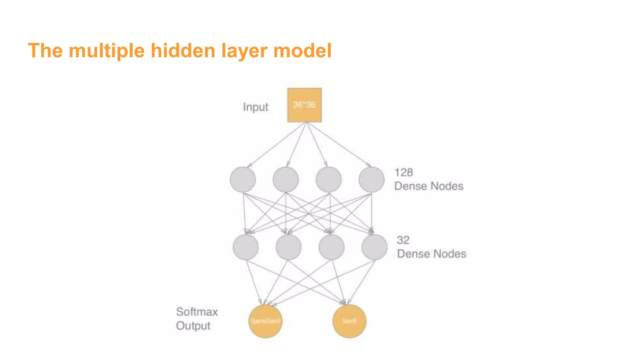
![The multiple hidden layer model
# Hidden layer 1
num_hidden1 = 256
W1 = tf.Variable(tf.truncated_normal([1296,num_hidden1],
stddev=1./math.sqrt(1296)))
b1 = tf.Variable(tf.constant(0.1,shape=[num_hidden1]))
h1 = tf.sigmoid(tf.matmul(x,W1) + b1)
# Hidden Layer 2
num_hidden2 = 64
W2 = tf.Variable(tf.truncated_normal([num_hidden1,
num_hidden2],stddev=2./math.sqrt(num_hidden1)))
b2 = tf.Variable(tf.constant(0.2,shape=[num_hidden2]))
h2 = tf.sigmoid(tf.matmul(h1,W2) + b2)
# Output Layer
W3 = tf.Variable(tf.truncated_normal([num_hidden2, 2],
stddev=1./math.sqrt(2)))
b3 = tf.Variable(tf.constant(0.1,shape=[2]))
# Just initialize
sess.run(tf.global_variables_initializer())
# Define model
y = tf.nn.softmax(tf.matmul(h2,W3) + b3)
### End model specification, begin training code](https://image.slidesharecdn.com/womeninai-fontclassificationwith5deeplearningmodelsusingtensorflow-190331022227/75/Font-classification-with-5-deep-learning-models-using-tensor-flow-13-2048.jpg)
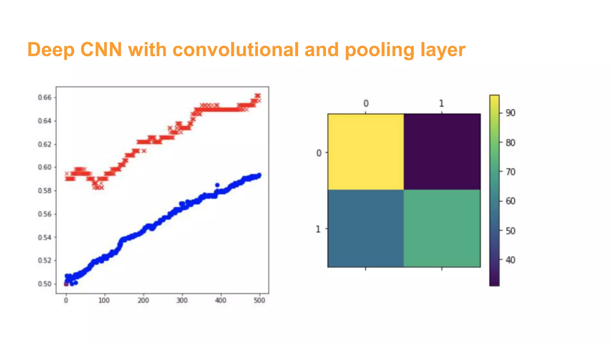
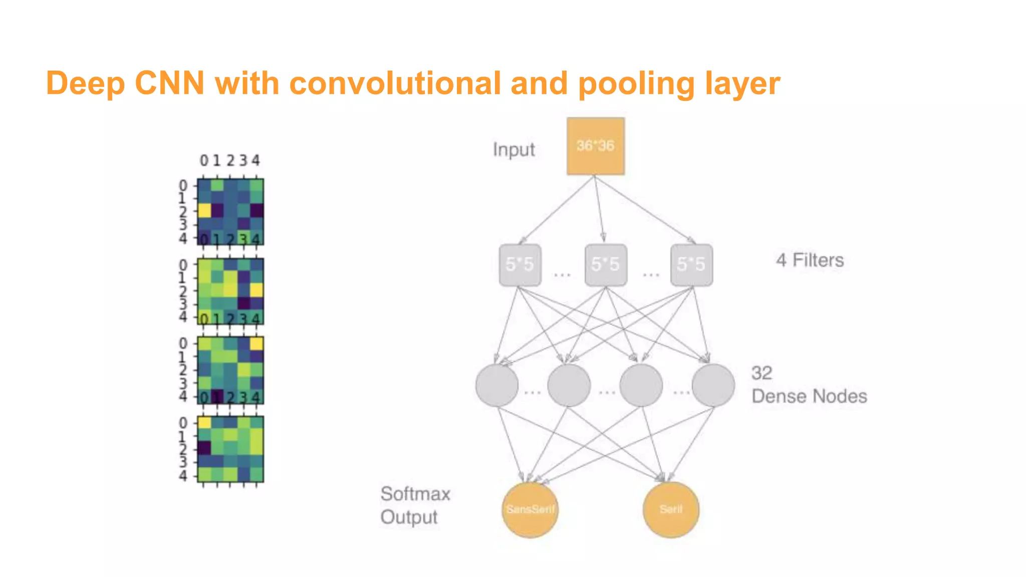
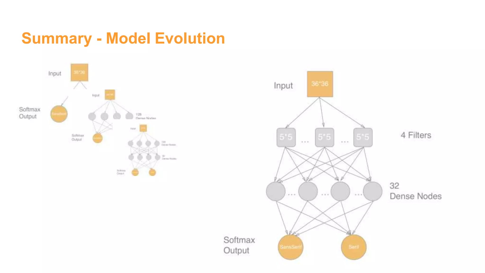
![Deep CNN with convolutional and pooling layer
# Conv layer 1
num_filters = 4
winx = 5
winy = 5
W1 = tf.Variable(tf.truncated_normal(
[winx, winy, 1 , num_filters],
stddev=1./math.sqrt(winx*winy)))
b1 = tf.Variable(tf.constant(0.1,
shape=[num_filters]))
# 5x5 convolution, pad with zeros on edges
xw = tf.nn.conv2d(x_im, W1,
strides=[1, 1, 1, 1],
padding='SAME')
h1 = tf.nn.relu(xw + b1)
# 2x2 Max pooling, no padding on edges
p1 = tf.nn.max_pool(h1, ksize=[1, 2, 2, 1],
strides=[1, 2, 2, 1], padding='VALID')
# Need to flatten convolutional output for use in dense layer
p1_size = np.product(
[s.value for s in p1.get_shape()[1:]])
p1f = tf.reshape(p1, [-1, p1_size ])
# Dense layer
num_hidden = 32
W2 = tf.Variable(tf.truncated_normal(
[p1_size, num_hidden],
stddev=2./math.sqrt(p1_size)))
b2 = tf.Variable(tf.constant(0.2,
shape=[num_hidden]))
h2 = tf.nn.relu(tf.matmul(p1f,W2) + b2)
# Output Layer
W3 = tf.Variable(tf.truncated_normal(
[num_hidden, 2],
stddev=1./math.sqrt(num_hidden)))
b3 = tf.Variable(tf.constant(0.1,shape=[2]))](https://image.slidesharecdn.com/womeninai-fontclassificationwith5deeplearningmodelsusingtensorflow-190331022227/75/Font-classification-with-5-deep-learning-models-using-tensor-flow-16-2048.jpg)
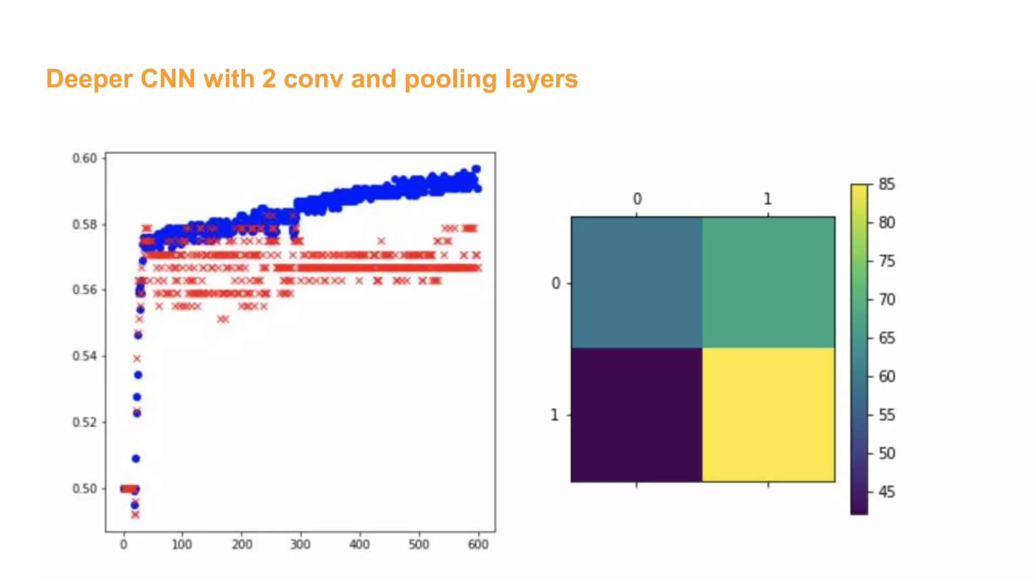
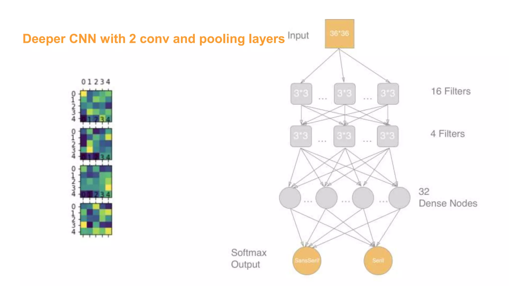
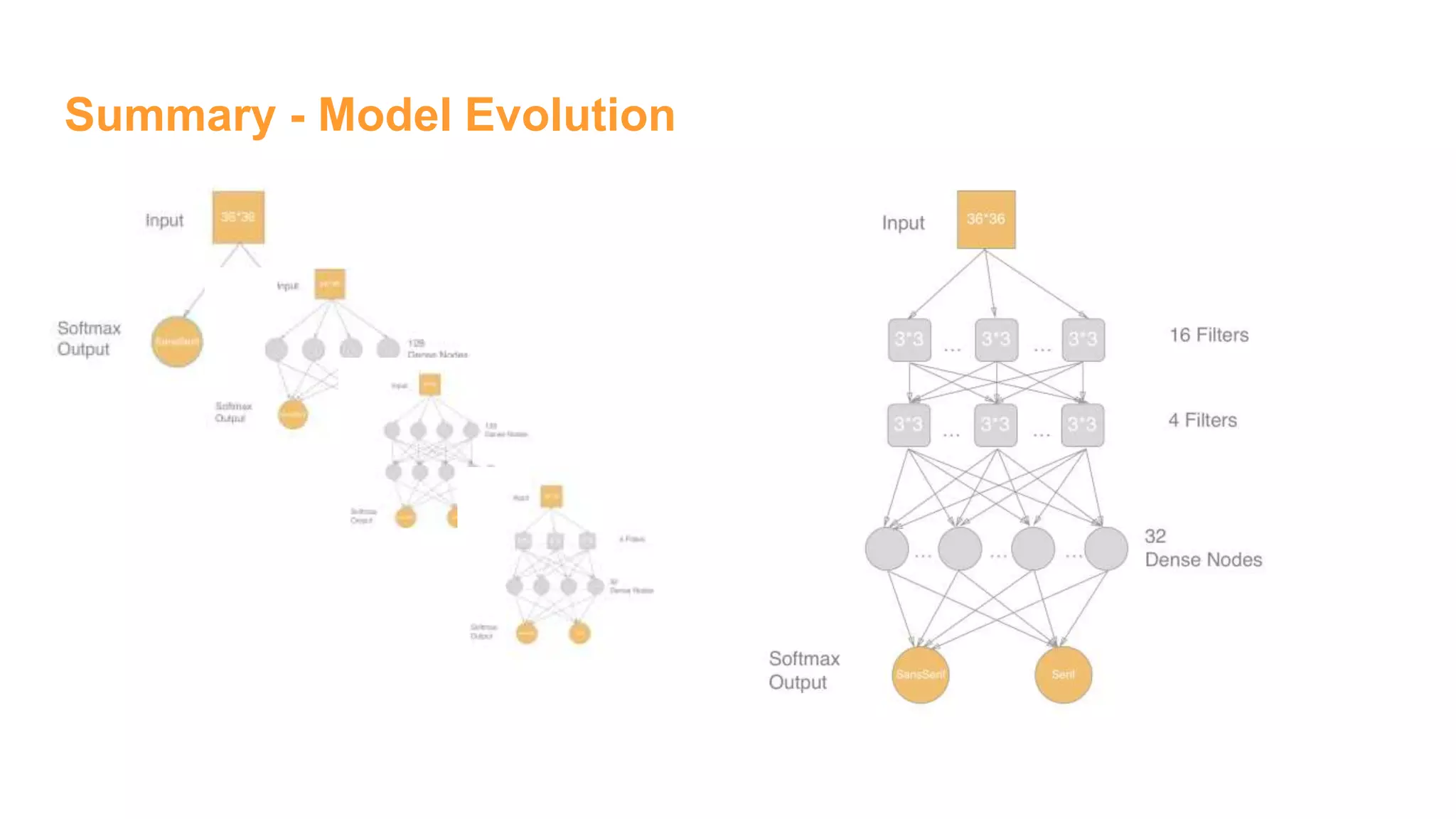
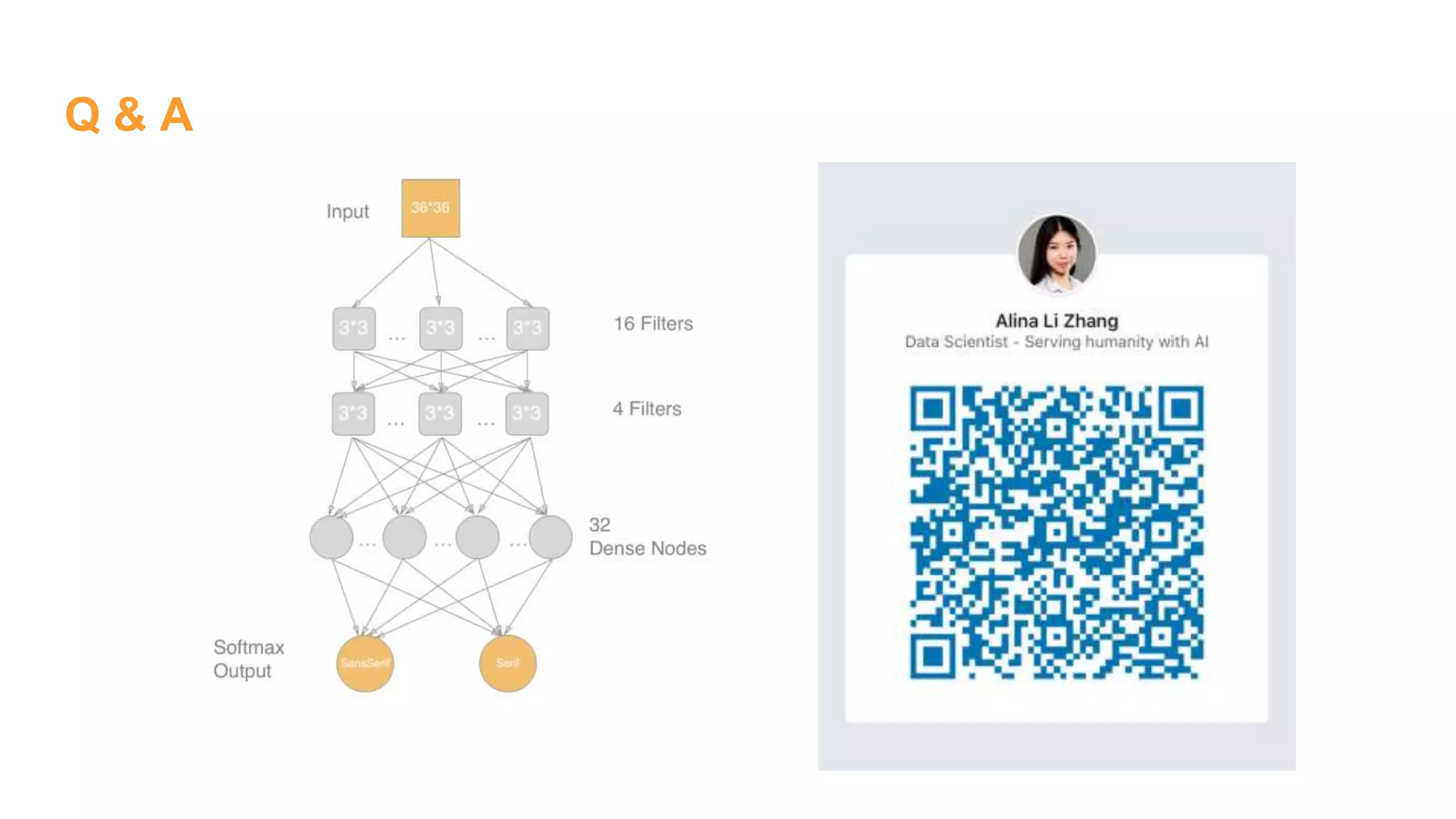
![Deeper CNN with 2 conv and pooling layers
# Conv layer 1
num_filters1 = 16
winx1 = 5
winy1 = 5
W1 = tf.Variable(tf.truncated_normal(
[winx1, winy1, 1 , num_filters1],
stddev=1./math.sqrt(winx1*winy1)))
b1 = tf.Variable(tf.constant(0.1,
shape=[num_filters1]))
# 5x5 convolution, pad with zeros on edges
xw = tf.nn.conv2d(x_im, W1,
strides=[1, 1, 1, 1],
padding='SAME')
h1 = tf.nn.relu(xw + b1)
# 2x2 Max pooling, no padding on edges
p1 = tf.nn.max_pool(h1, ksize=[1, 2, 2, 1],
strides=[1, 2, 2, 1], padding='VALID')
Conv layer 2
num_filters2 = 4
winx2 = 3
winy2 = 3
W2 = tf.Variable(tf.truncated_normal(
[winx2, winy2, num_filters1, num_filters2],
stddev=1./math.sqrt(winx2*winy2)))
b2 = tf.Variable(tf.constant(0.1,
shape=[num_filters2]))
# 3x3 convolution, pad with zeros on edges
p1w2 = tf.nn.conv2d(p1, W2,
strides=[1, 1, 1, 1], padding='SAME')
h1 = tf.nn.relu(p1w2 + b2)
# 2x2 Max pooling, no padding on edges
p2 = tf.nn.max_pool(h1, ksize=[1, 2, 2, 1],
strides=[1, 2, 2, 1], padding='VALID')](https://image.slidesharecdn.com/womeninai-fontclassificationwith5deeplearningmodelsusingtensorflow-190331022227/75/Font-classification-with-5-deep-learning-models-using-tensor-flow-19-2048.jpg)
![Deeper CNN with 2 conv and pooling layers
# Need to flatten convolutional output
p2_size = np.product(
[s.value for s in p2.get_shape()[1:]])
p2f = tf.reshape(p2, [-1, p2_size ])
# Dense layer
num_hidden = 32
W3 = tf.Variable(tf.truncated_normal(
[p2_size, num_hidden],
stddev=2./math.sqrt(p2_size)))
b3 = tf.Variable(tf.constant(0.2,
shape=[num_hidden]))
h3 = tf.nn.relu(tf.matmul(p2f,W3) + b3)
# Output Layer
W4 = tf.Variable(tf.truncated_normal(
[num_hidden, 2],
stddev=1./math.sqrt(num_hidden)))
b4 = tf.Variable(tf.constant(0.1,shape=[2]))
# Just initialize
sess.run(tf.global_variables_initializer())
# Define model
y = tf.nn.softmax(tf.matmul(h3,W4) + b4)](https://image.slidesharecdn.com/womeninai-fontclassificationwith5deeplearningmodelsusingtensorflow-190331022227/75/Font-classification-with-5-deep-learning-models-using-tensor-flow-20-2048.jpg)
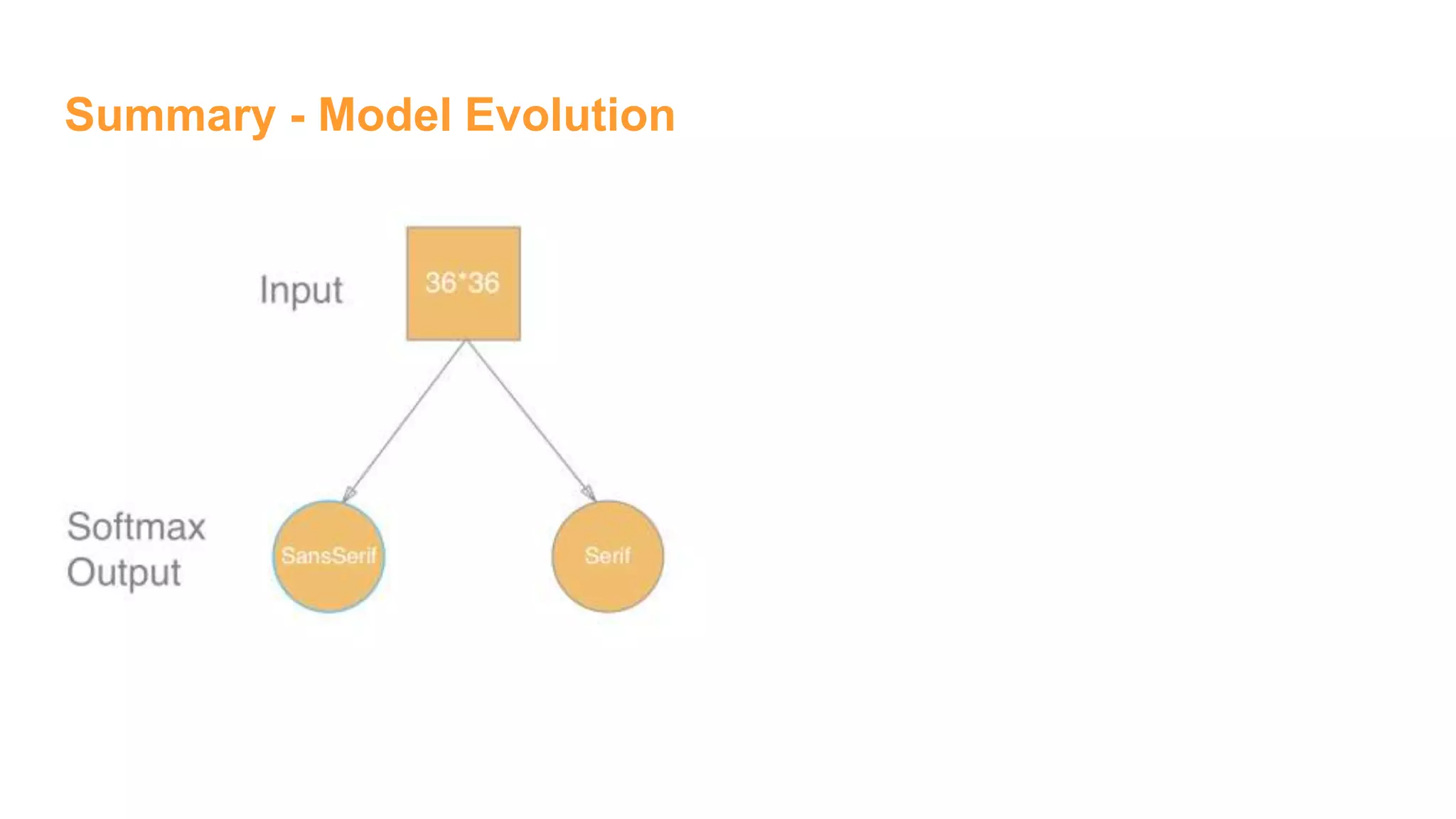


![Logistic regression model - build model
sess = tf.InteractiveSession()
# These will be inputs
## Input pixels, flattened
x = tf.placeholder("float", [None, 1296])
## Known labels
y_ = tf.placeholder("float", [None,2])
# Variables
W = tf.Variable(tf.zeros([1296,2]))
b = tf.Variable(tf.zeros([2]))
# Just initialize
sess.run(tf.global_variables_initializer())
# Define model
y = tf.nn.softmax(tf.matmul(x,W) + b)
### End model specification, begin training code](https://crownmelresort.com/image.slidesharecdn.com/womeninai-fontclassificationwith5deeplearningmodelsusingtensorflow-190331022227/75/Font-classification-with-5-deep-learning-models-using-tensor-flow-7-2048.jpg)


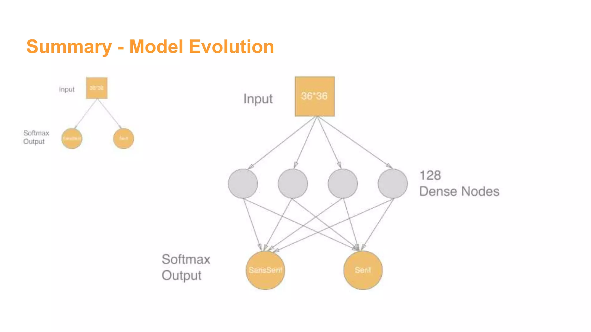
![Single hidden layer model
# Hidden layer
num_hidden = 128
W1 = tf.Variable(tf.truncated_normal([1296, num_hidden],
stddev=1./math.sqrt(1296)))
b1 = tf.Variable(tf.constant(0.1,shape=[num_hidden]))
h1 = tf.sigmoid(tf.matmul(x,W1) + b1)
# Output Layer
W2 = tf.Variable(tf.truncated_normal([num_hidden, 2],
stddev=1./math.sqrt(2)))
b2 = tf.Variable(tf.constant(0.1,shape=[2]))
# Just initialize
sess.run(tf.global_variables_initializer())
# Define model
y = tf.nn.softmax(tf.matmul(h1,W2) + b2)
### End model specification, begin training code
# Actually train
epochs = 20000
train_acc = np.zeros(epochs//10)
test_acc = np.zeros(epochs//10)
for i in tqdm(range(epochs), ascii=True):
if i % 10 == 0:
# Check accuracy on train set
A = accuracy.eval(feed_dict={
x: train_dataset,
y_: train_labels})
train_acc[i//10] = A
# And now the validation set
A = accuracy.eval(feed_dict={
x: valid_dataset,
y_: valid_labels})
test_acc[i//10] = A
train_step.run(feed_dict={
x: train_dataset,
y_: train_labels})](https://crownmelresort.com/image.slidesharecdn.com/womeninai-fontclassificationwith5deeplearningmodelsusingtensorflow-190331022227/75/Font-classification-with-5-deep-learning-models-using-tensor-flow-10-2048.jpg)


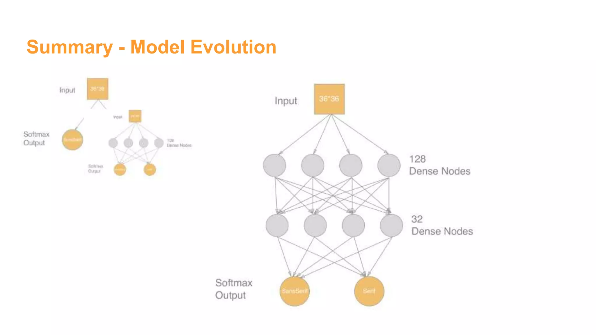
![The multiple hidden layer model
# Hidden layer 1
num_hidden1 = 256
W1 = tf.Variable(tf.truncated_normal([1296,num_hidden1],
stddev=1./math.sqrt(1296)))
b1 = tf.Variable(tf.constant(0.1,shape=[num_hidden1]))
h1 = tf.sigmoid(tf.matmul(x,W1) + b1)
# Hidden Layer 2
num_hidden2 = 64
W2 = tf.Variable(tf.truncated_normal([num_hidden1,
num_hidden2],stddev=2./math.sqrt(num_hidden1)))
b2 = tf.Variable(tf.constant(0.2,shape=[num_hidden2]))
h2 = tf.sigmoid(tf.matmul(h1,W2) + b2)
# Output Layer
W3 = tf.Variable(tf.truncated_normal([num_hidden2, 2],
stddev=1./math.sqrt(2)))
b3 = tf.Variable(tf.constant(0.1,shape=[2]))
# Just initialize
sess.run(tf.global_variables_initializer())
# Define model
y = tf.nn.softmax(tf.matmul(h2,W3) + b3)
### End model specification, begin training code](https://crownmelresort.com/image.slidesharecdn.com/womeninai-fontclassificationwith5deeplearningmodelsusingtensorflow-190331022227/75/Font-classification-with-5-deep-learning-models-using-tensor-flow-13-2048.jpg)


![Deep CNN with convolutional and pooling layer
# Conv layer 1
num_filters = 4
winx = 5
winy = 5
W1 = tf.Variable(tf.truncated_normal(
[winx, winy, 1 , num_filters],
stddev=1./math.sqrt(winx*winy)))
b1 = tf.Variable(tf.constant(0.1,
shape=[num_filters]))
# 5x5 convolution, pad with zeros on edges
xw = tf.nn.conv2d(x_im, W1,
strides=[1, 1, 1, 1],
padding='SAME')
h1 = tf.nn.relu(xw + b1)
# 2x2 Max pooling, no padding on edges
p1 = tf.nn.max_pool(h1, ksize=[1, 2, 2, 1],
strides=[1, 2, 2, 1], padding='VALID')
# Need to flatten convolutional output for use in dense layer
p1_size = np.product(
[s.value for s in p1.get_shape()[1:]])
p1f = tf.reshape(p1, [-1, p1_size ])
# Dense layer
num_hidden = 32
W2 = tf.Variable(tf.truncated_normal(
[p1_size, num_hidden],
stddev=2./math.sqrt(p1_size)))
b2 = tf.Variable(tf.constant(0.2,
shape=[num_hidden]))
h2 = tf.nn.relu(tf.matmul(p1f,W2) + b2)
# Output Layer
W3 = tf.Variable(tf.truncated_normal(
[num_hidden, 2],
stddev=1./math.sqrt(num_hidden)))
b3 = tf.Variable(tf.constant(0.1,shape=[2]))](https://crownmelresort.com/image.slidesharecdn.com/womeninai-fontclassificationwith5deeplearningmodelsusingtensorflow-190331022227/75/Font-classification-with-5-deep-learning-models-using-tensor-flow-16-2048.jpg)


![Deeper CNN with 2 conv and pooling layers
# Conv layer 1
num_filters1 = 16
winx1 = 5
winy1 = 5
W1 = tf.Variable(tf.truncated_normal(
[winx1, winy1, 1 , num_filters1],
stddev=1./math.sqrt(winx1*winy1)))
b1 = tf.Variable(tf.constant(0.1,
shape=[num_filters1]))
# 5x5 convolution, pad with zeros on edges
xw = tf.nn.conv2d(x_im, W1,
strides=[1, 1, 1, 1],
padding='SAME')
h1 = tf.nn.relu(xw + b1)
# 2x2 Max pooling, no padding on edges
p1 = tf.nn.max_pool(h1, ksize=[1, 2, 2, 1],
strides=[1, 2, 2, 1], padding='VALID')
Conv layer 2
num_filters2 = 4
winx2 = 3
winy2 = 3
W2 = tf.Variable(tf.truncated_normal(
[winx2, winy2, num_filters1, num_filters2],
stddev=1./math.sqrt(winx2*winy2)))
b2 = tf.Variable(tf.constant(0.1,
shape=[num_filters2]))
# 3x3 convolution, pad with zeros on edges
p1w2 = tf.nn.conv2d(p1, W2,
strides=[1, 1, 1, 1], padding='SAME')
h1 = tf.nn.relu(p1w2 + b2)
# 2x2 Max pooling, no padding on edges
p2 = tf.nn.max_pool(h1, ksize=[1, 2, 2, 1],
strides=[1, 2, 2, 1], padding='VALID')](https://crownmelresort.com/image.slidesharecdn.com/womeninai-fontclassificationwith5deeplearningmodelsusingtensorflow-190331022227/75/Font-classification-with-5-deep-learning-models-using-tensor-flow-19-2048.jpg)
![Deeper CNN with 2 conv and pooling layers
# Need to flatten convolutional output
p2_size = np.product(
[s.value for s in p2.get_shape()[1:]])
p2f = tf.reshape(p2, [-1, p2_size ])
# Dense layer
num_hidden = 32
W3 = tf.Variable(tf.truncated_normal(
[p2_size, num_hidden],
stddev=2./math.sqrt(p2_size)))
b3 = tf.Variable(tf.constant(0.2,
shape=[num_hidden]))
h3 = tf.nn.relu(tf.matmul(p2f,W3) + b3)
# Output Layer
W4 = tf.Variable(tf.truncated_normal(
[num_hidden, 2],
stddev=1./math.sqrt(num_hidden)))
b4 = tf.Variable(tf.constant(0.1,shape=[2]))
# Just initialize
sess.run(tf.global_variables_initializer())
# Define model
y = tf.nn.softmax(tf.matmul(h3,W4) + b4)](https://crownmelresort.com/image.slidesharecdn.com/womeninai-fontclassificationwith5deeplearningmodelsusingtensorflow-190331022227/75/Font-classification-with-5-deep-learning-models-using-tensor-flow-20-2048.jpg)


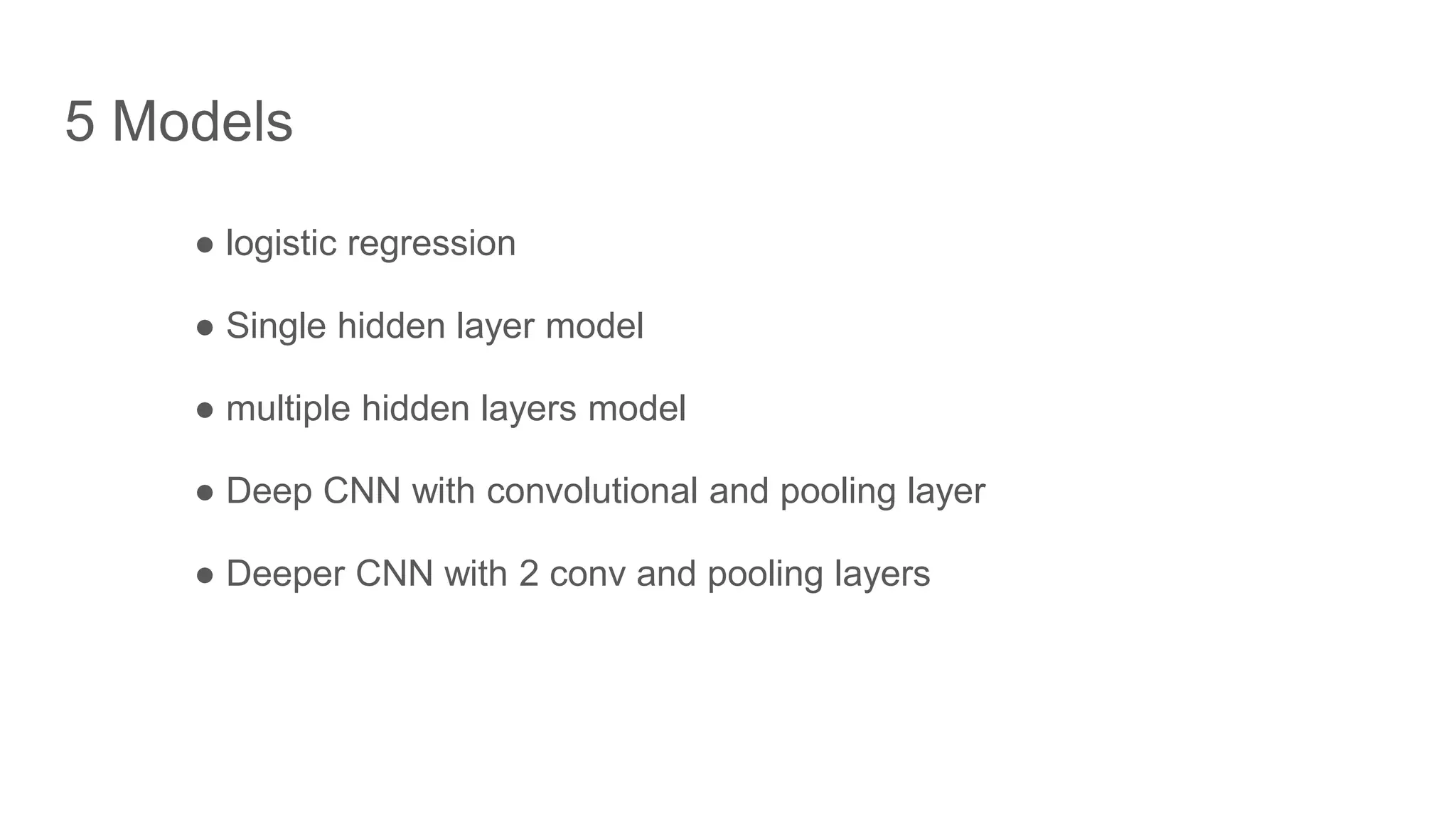
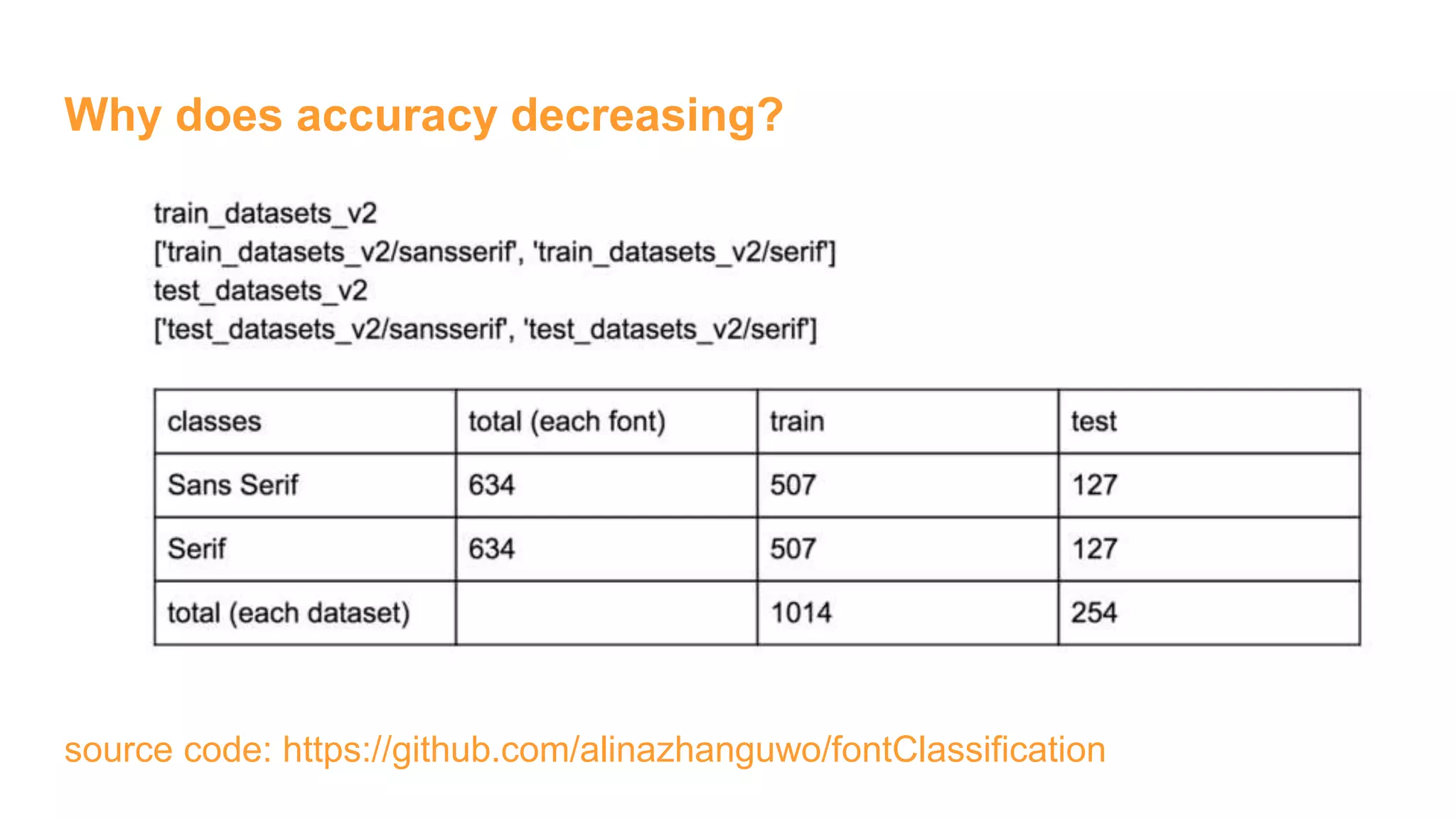
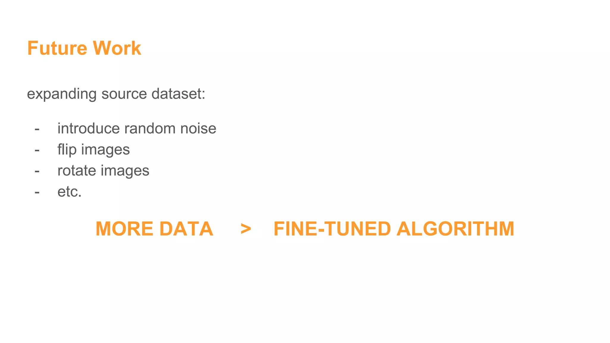
The document details the development of font classification models using five different deep learning architectures in TensorFlow. It covers the processes of data engineering, building, and training various models, including logistic regression, single and multiple hidden layer networks, and convolutional neural networks (CNNs). Additionally, it discusses future work to improve model accuracy through expanding the dataset with diverse transformations.

![[신경망기초] 합성곱신경망](https://cdn.slidesharecdn.com/ss_thumbnails/2-180604135842-thumbnail.jpg?width=640&height=640&fit=bounds)

![[신경망기초]오류역전파알고리즘구현](https://cdn.slidesharecdn.com/ss_thumbnails/nn-190319093725-thumbnail.jpg?width=640&height=640&fit=bounds)


![[Redis Released]- FalkorDB - Redis + Graph Agentic Memory’s Secret Sauce](https://cdn.slidesharecdn.com/ss_thumbnails/redisreleased-falkordbslidedeck-1125-251115194922-e1c0046b-thumbnail.jpg?width=640&height=640&fit=bounds)


