The document provides an overview of digital image processing, detailing its fundamentals, components, and methodologies. It covers key concepts such as image acquisition, enhancement, and recognition, as well as the importance of sampling and quantization in converting continuous images to digital form. Additionally, it discusses the relationships between image processing, image analysis, and computer vision, emphasizing their interconnectedness.

![Representing Digital Images
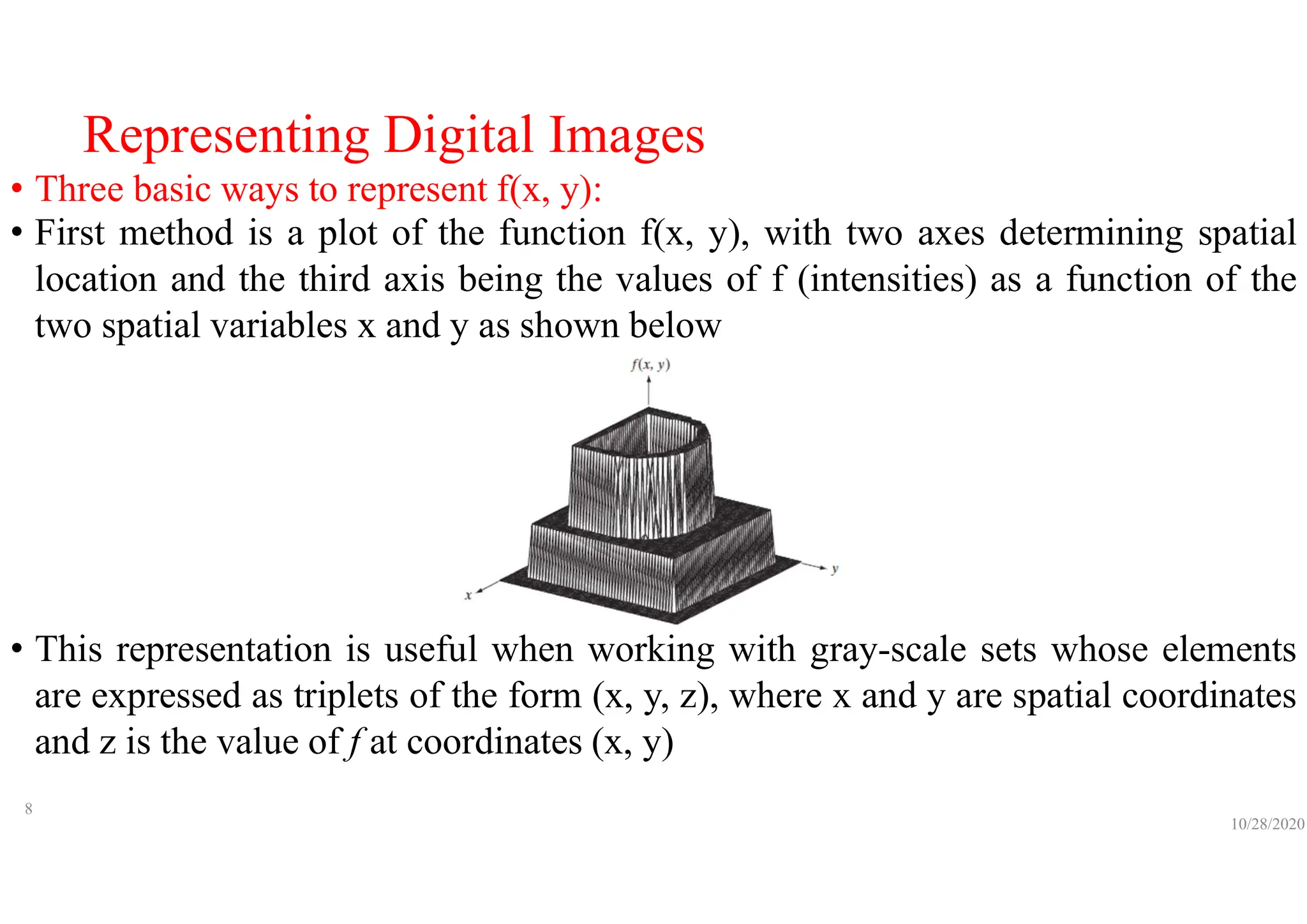
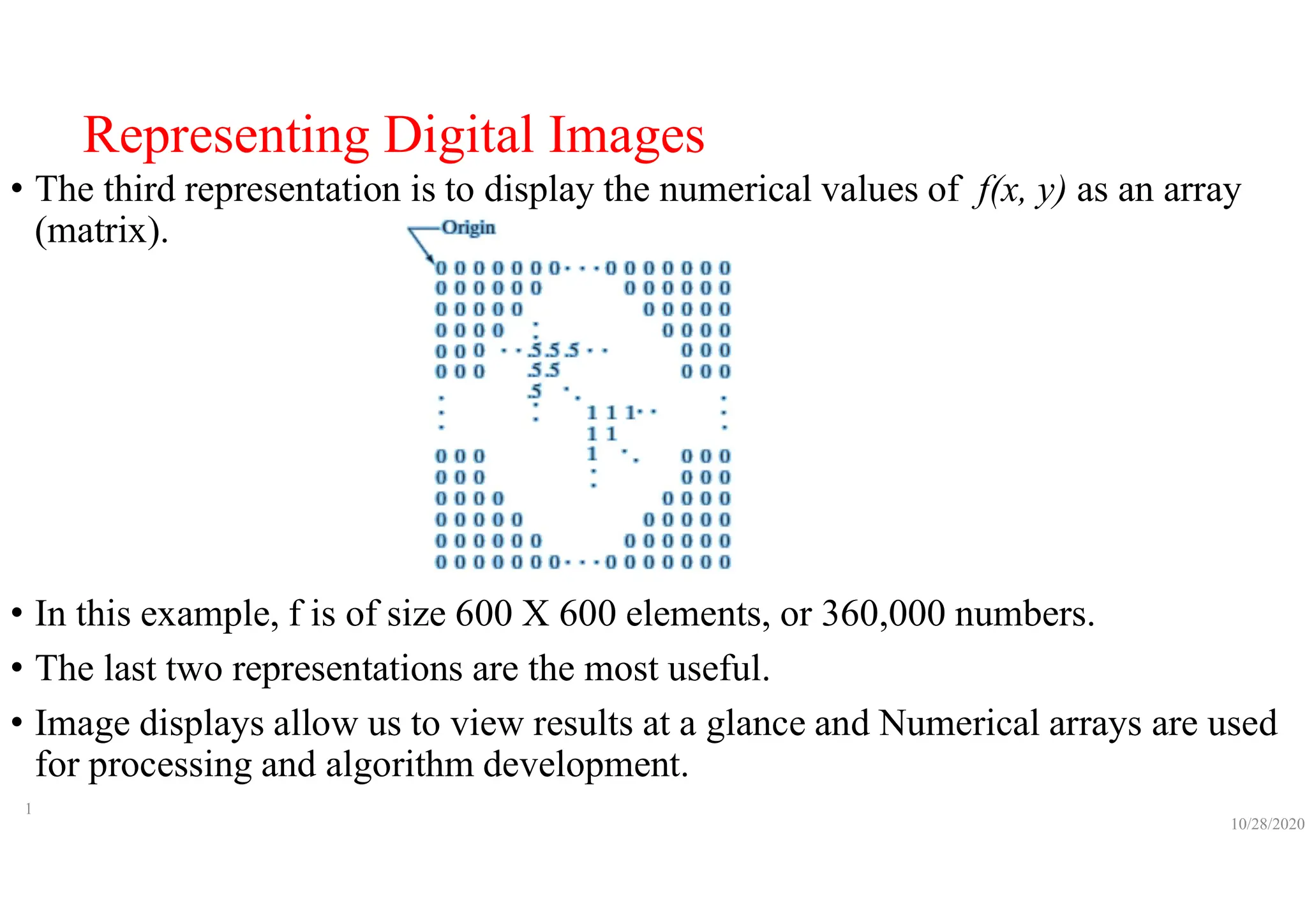
• Second method is as shown below
• This is much more common.
• Here, the intensity of each point is proportional to the value of f at that point.
• In this figure, there are only three equally spaced intensity values.
• If the intensity is normalized to the interval [0, 1], then each point in the image has
the value 0, 0.5, or 1.
• A monitor or printer simply converts these three values to black, gray, or white,
respectively
10/28/2020
9](https://image.slidesharecdn.com/imageprocessingppt-240726093651-137f8085/75/DIGITAL-image-processing-for-6th-sem-students-45-2048.jpg)

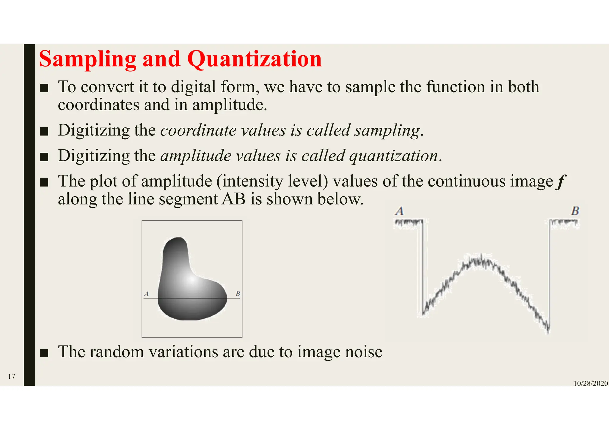
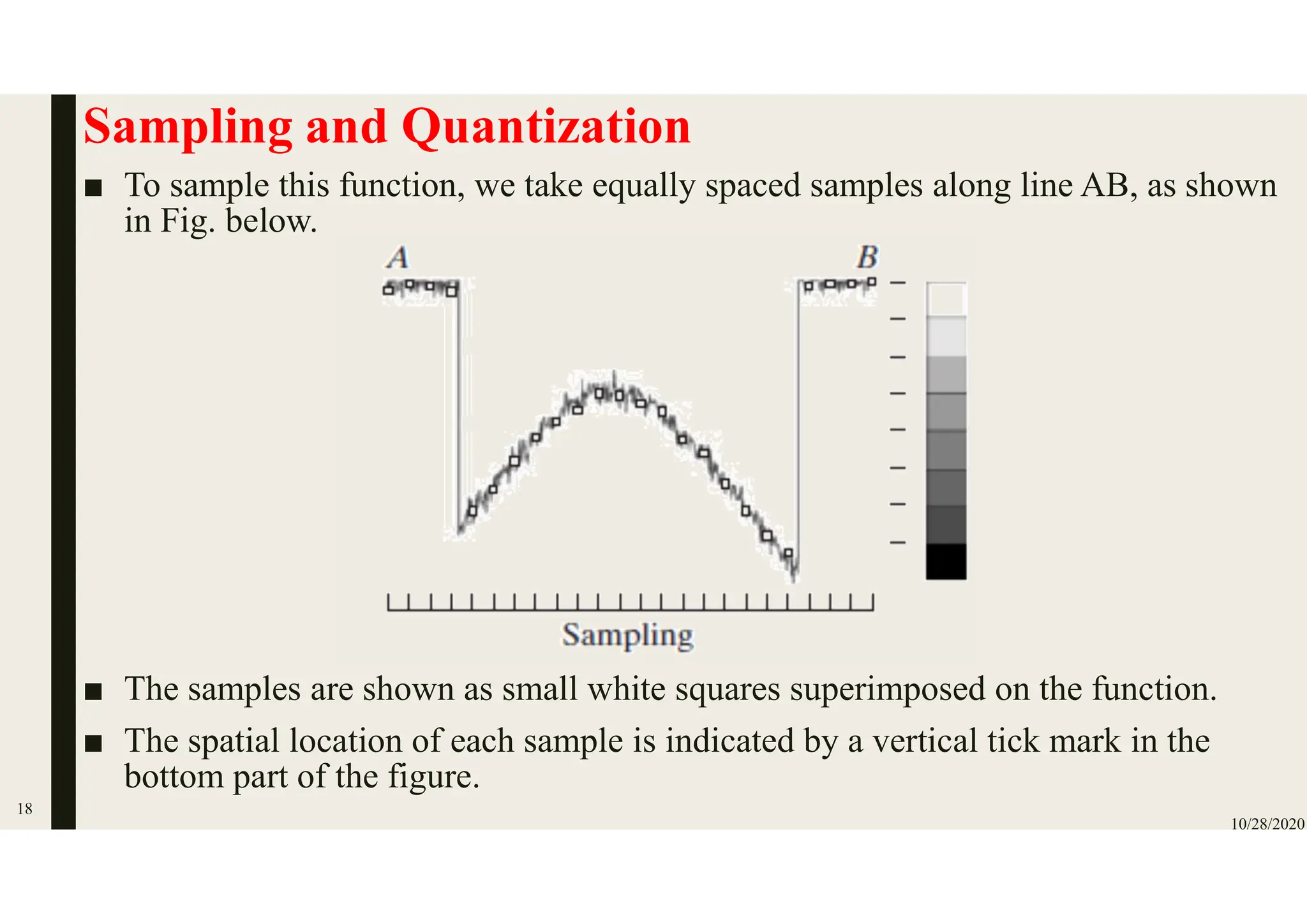
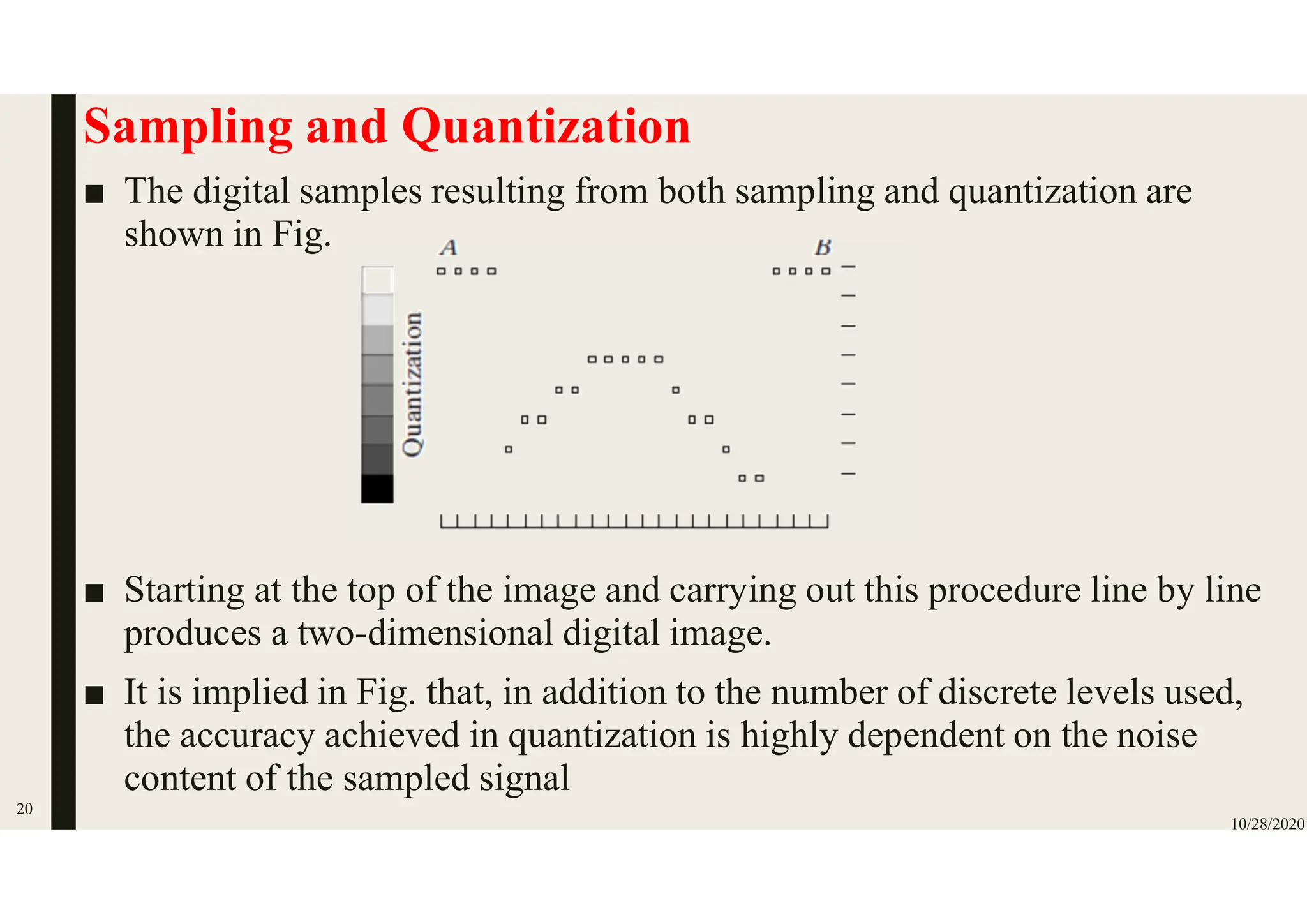
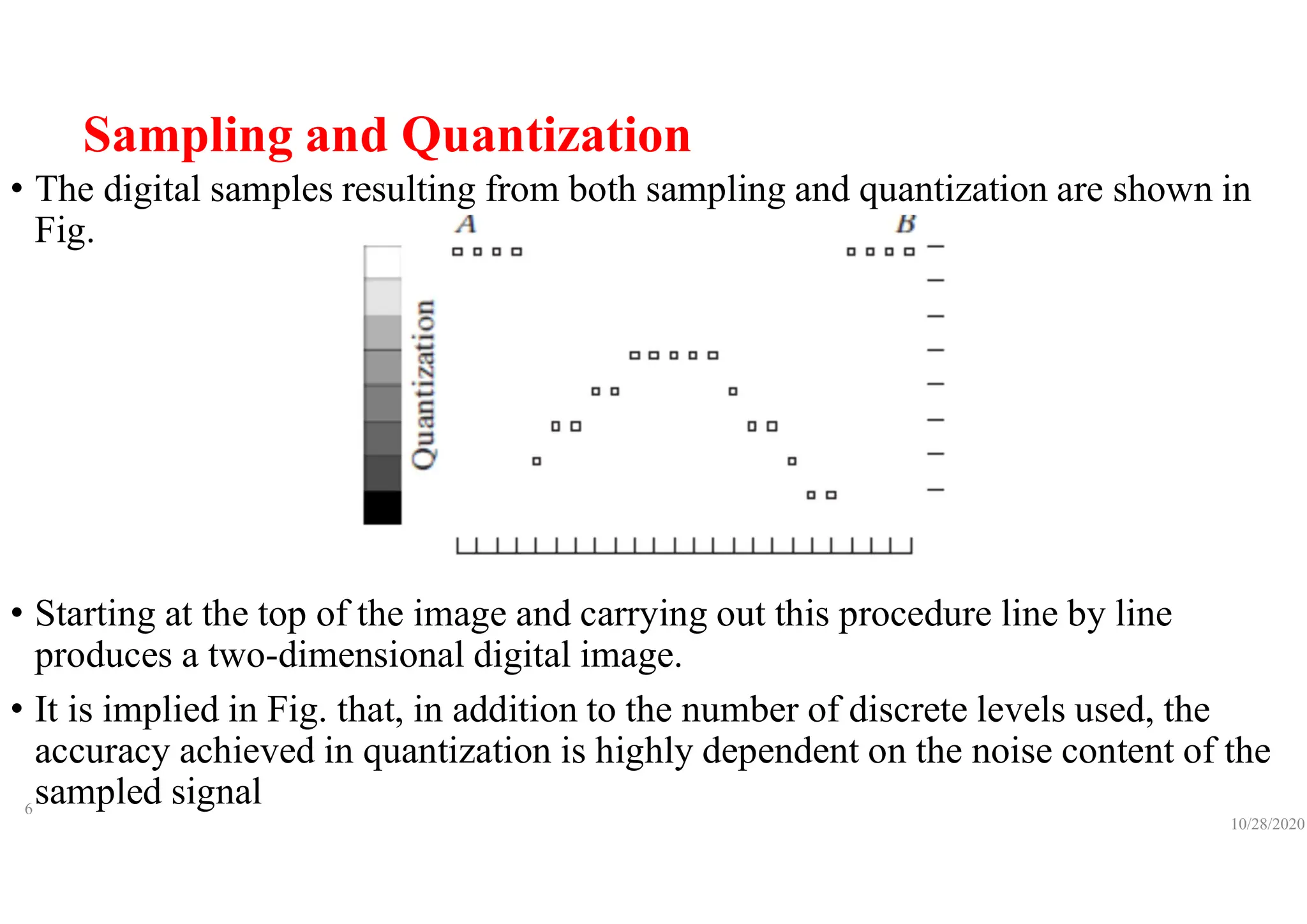
![Sampling and Quantization
• We assume that the discrete levels are equally spaced and that they are
integers in the interval [0,L-1]
• Sometimes, the range of values spanned by the gray scale is referred to
informally as the dynamic range.
• This is a term used in different ways in different fields.
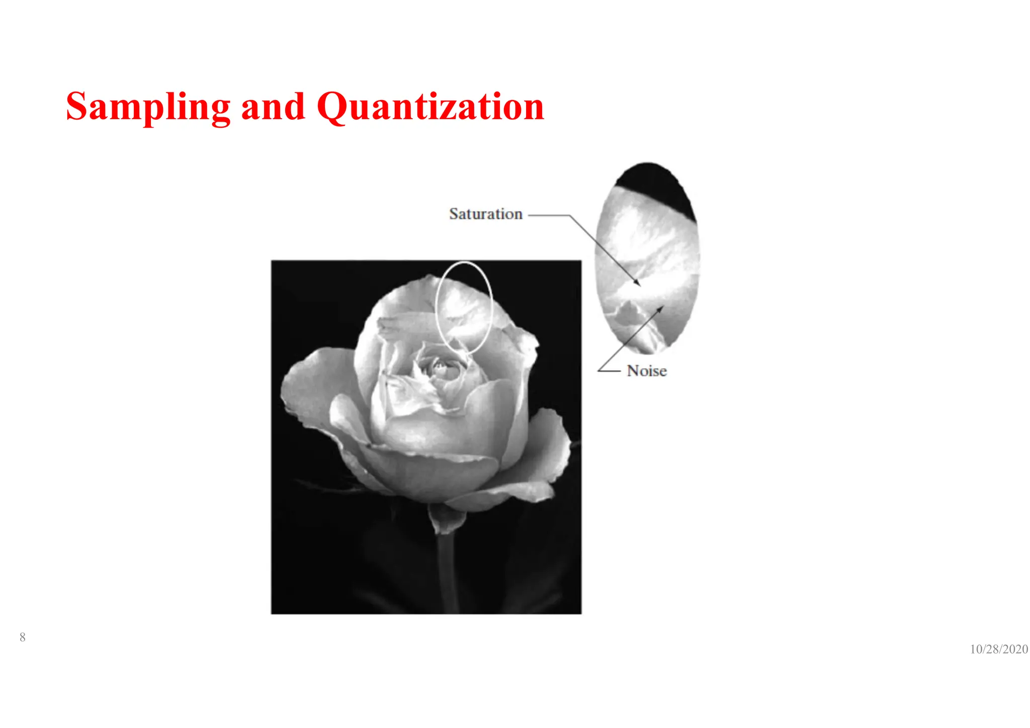
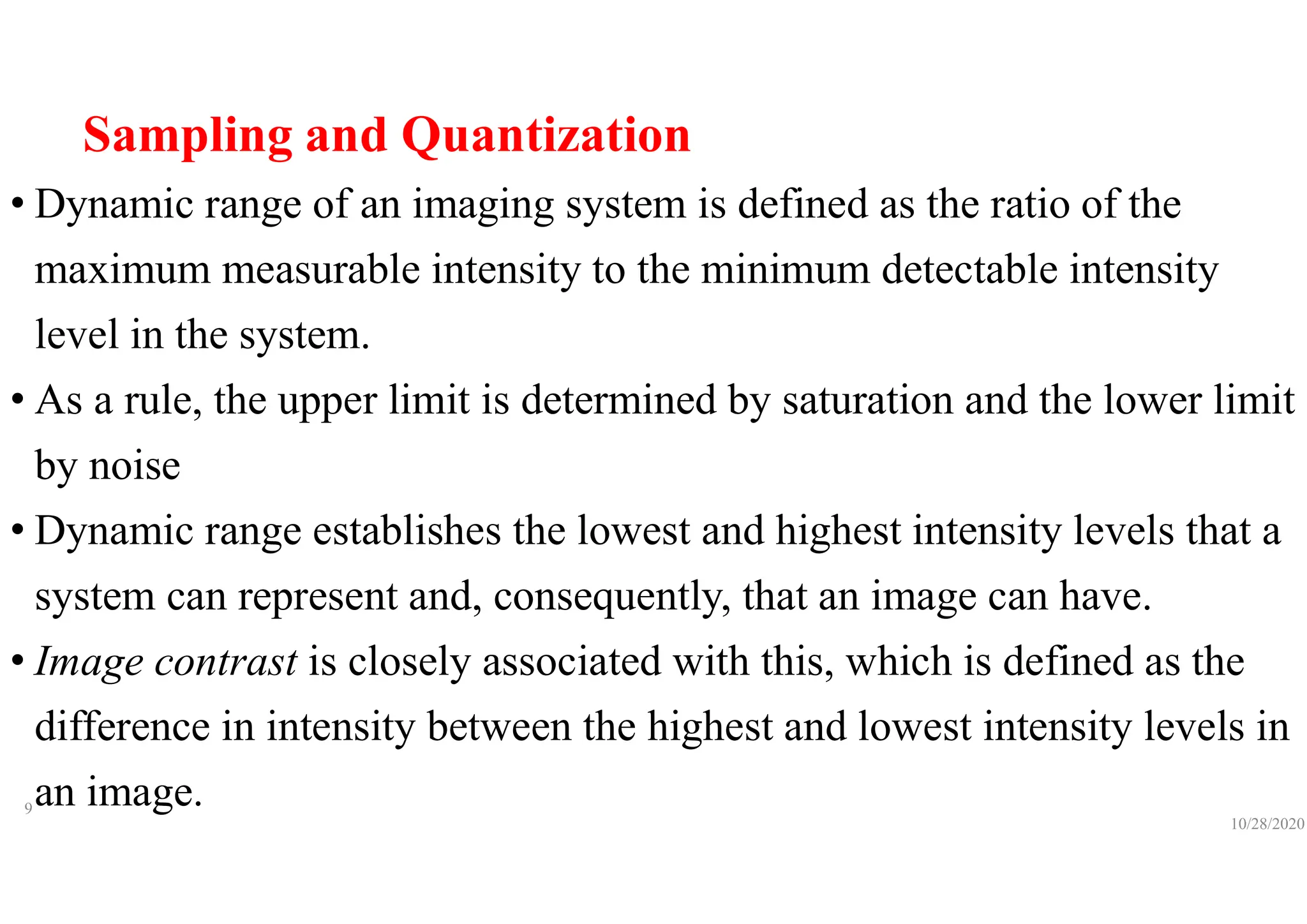
• We define the dynamic range of an imaging system to be the ratio of the
maximum measurable intensity to the minimum detectable intensity
level in the system.
• As a rule, the upper limit is determined by saturation and the lower limit
by noise
10/28/2020
6](https://image.slidesharecdn.com/imageprocessingppt-240726093651-137f8085/75/DIGITAL-image-processing-for-6th-sem-students-52-2048.jpg)
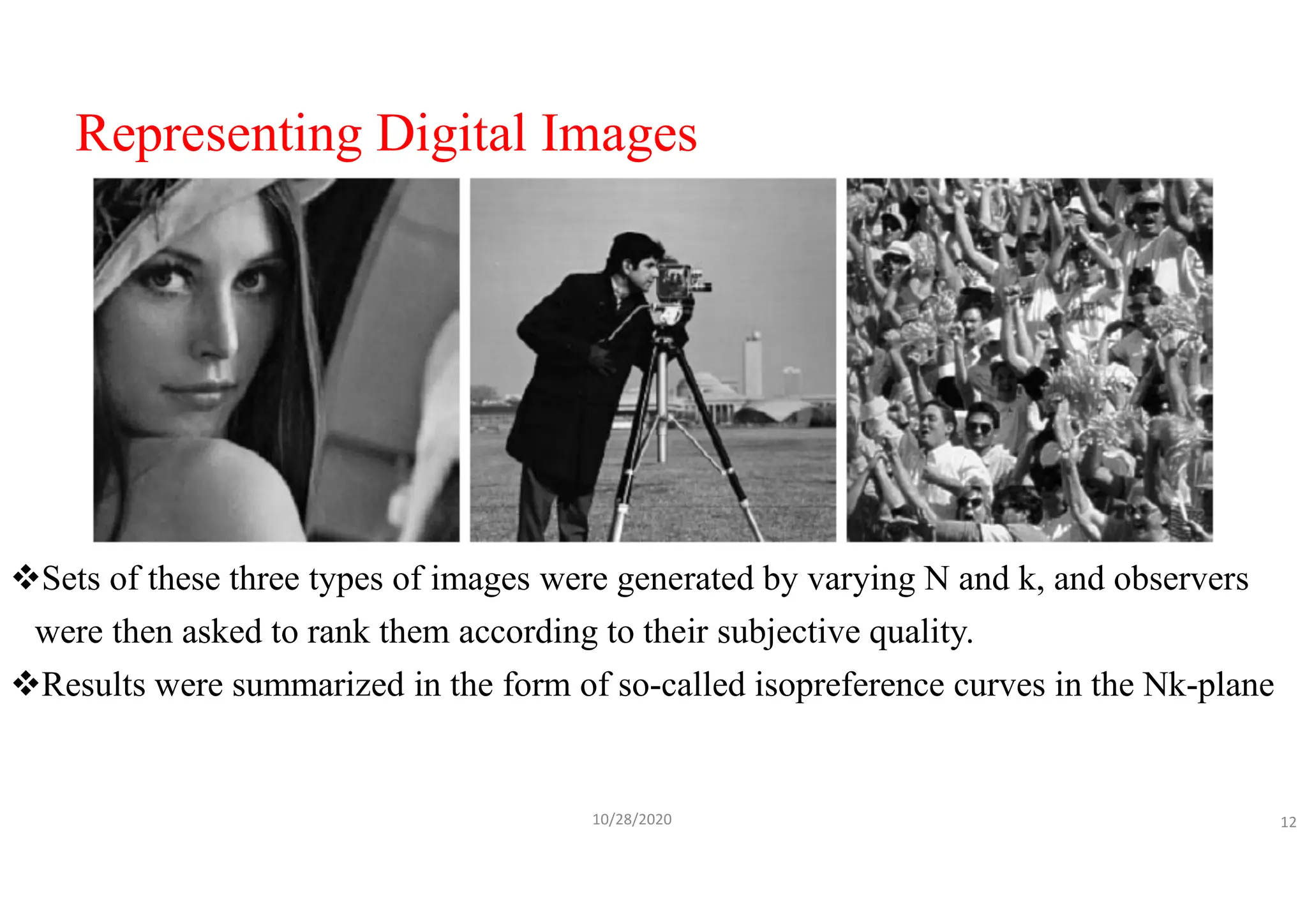
![Representing Digital Images
The results in previous two examples illustrate the effects produced on image
quality by varying N and k independently.
However, these results only partially answer the question of how varying N and k
affects images
Because we have not considered yet any relationships that might exist between
these two parameters.
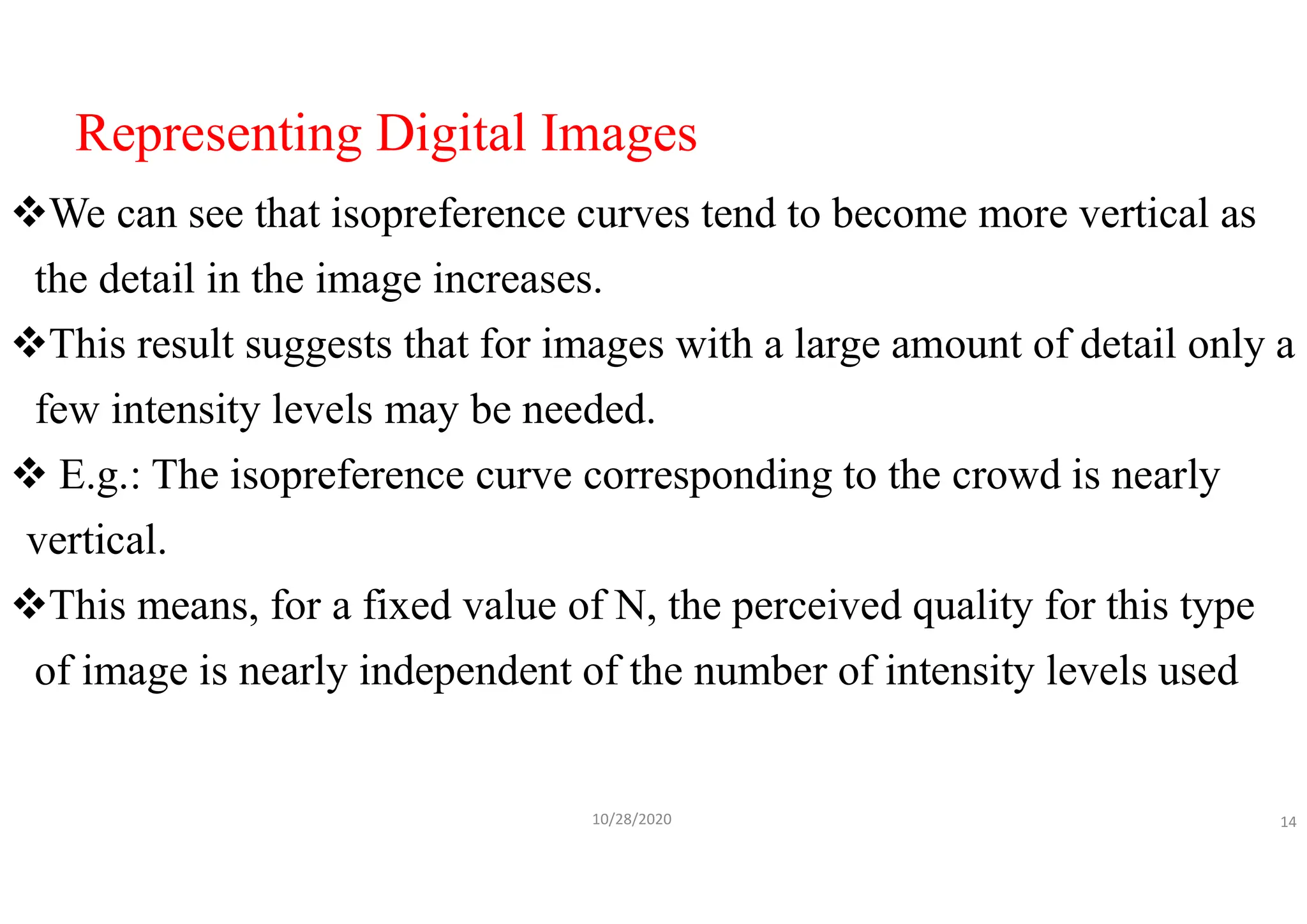
An early study by Huang [1965] attempted to quantify experimentally the effects
on image quality produced by varying N and k simultaneously.
The experiment consisted of a set of subjective tests on images which have very
little detail, moderate detail and large amount of details
10/28/2020 11](https://image.slidesharecdn.com/imageprocessingppt-240726093651-137f8085/75/DIGITAL-image-processing-for-6th-sem-students-70-2048.jpg)
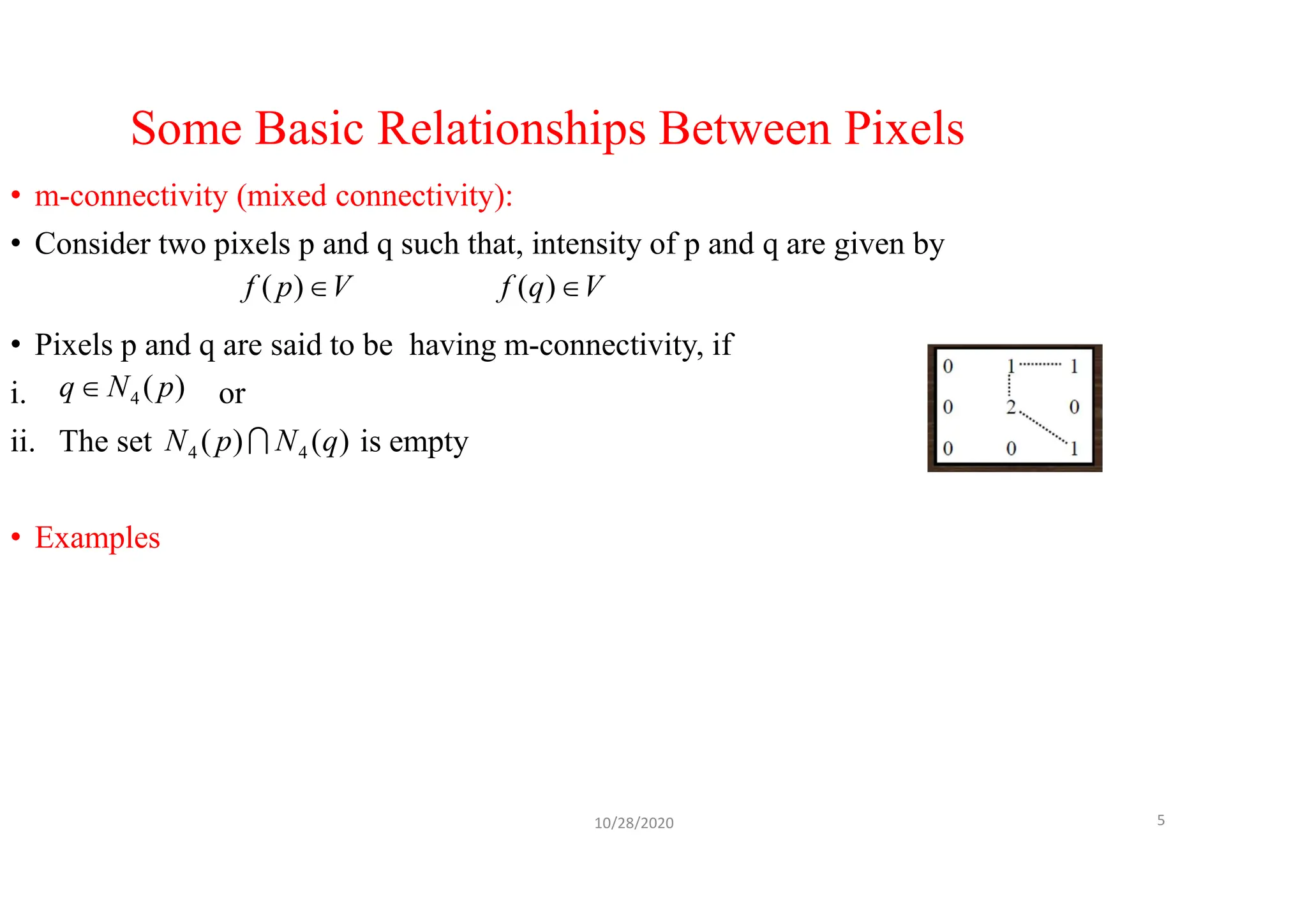

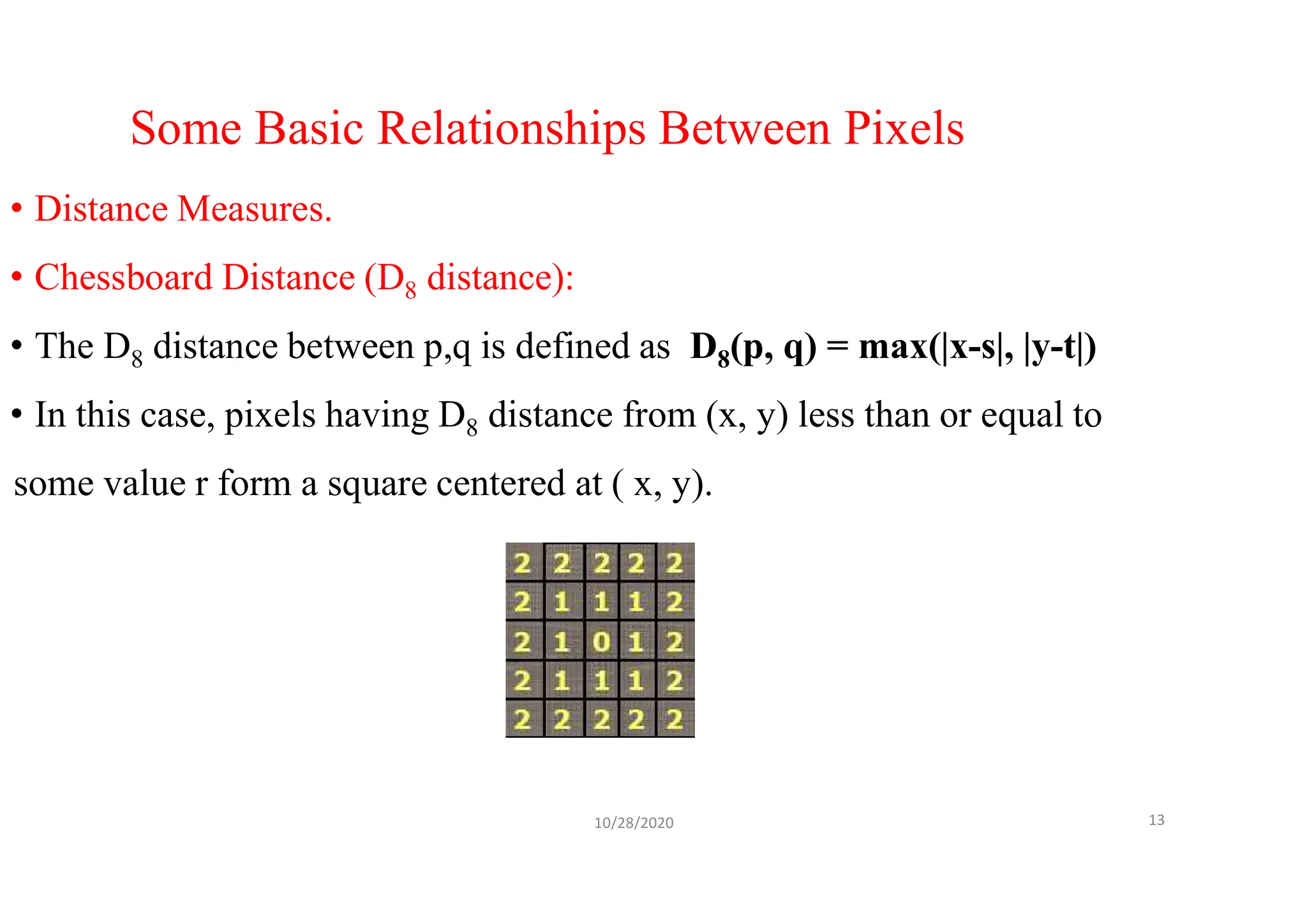
![Some Basic Relationships Between Pixels
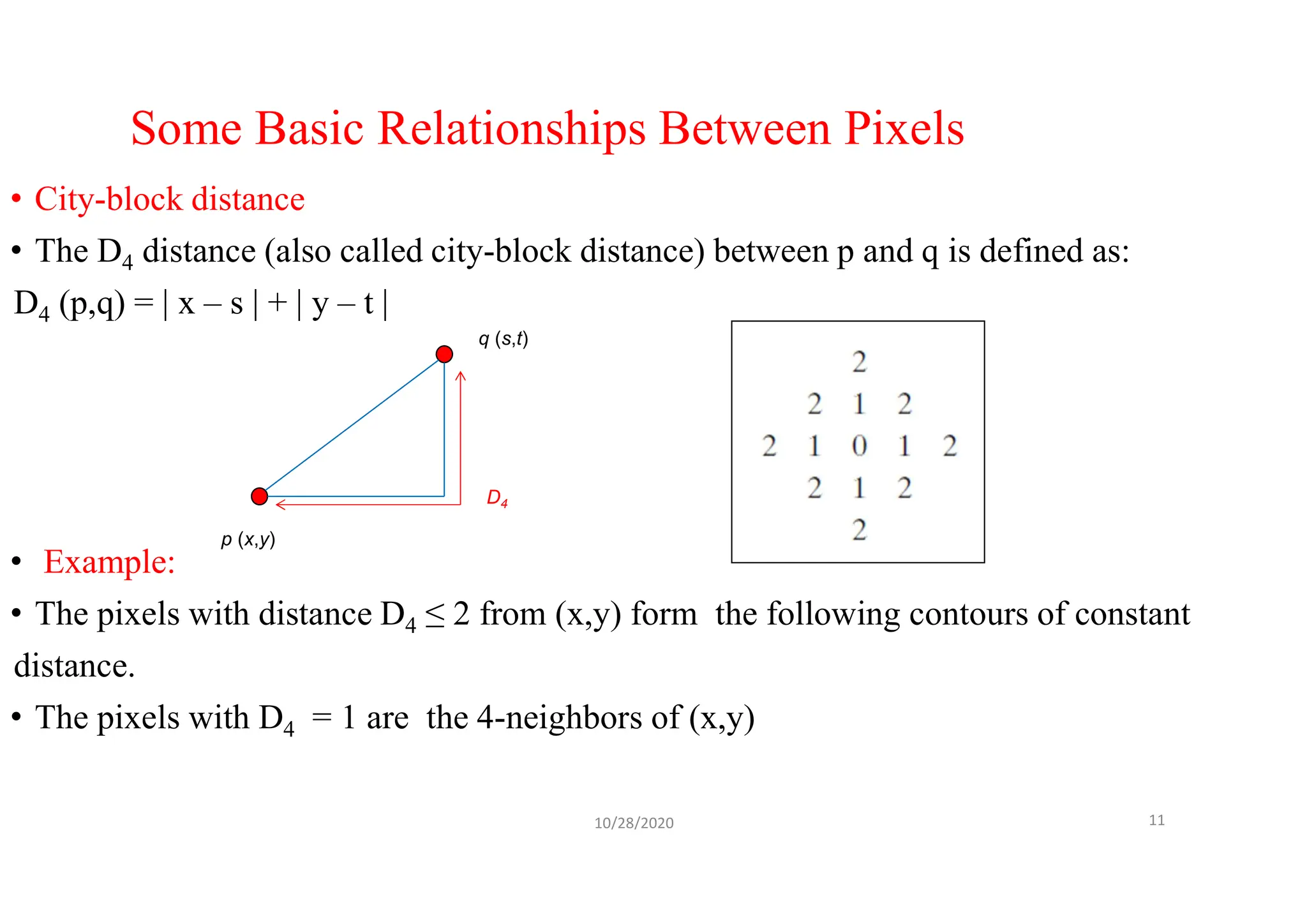
• Distance Measures
• Consider three pixels p, q, and z, with coordinates (x, y), (s, t), and (v, w), respectively
• The distance between any two points can be calculated as distance metric or distance
measure
• But it must satisfy the following properties
• The Euclidean distance between p and q is defined as
• De (p,q) = [(x – s)2 + (y - t)2]1/2
10/28/2020 10
p (x,y)
q (s,t)](https://image.slidesharecdn.com/imageprocessingppt-240726093651-137f8085/75/DIGITAL-image-processing-for-6th-sem-students-96-2048.jpg)


![Representing Digital Images
• Second method is as shown below
• This is much more common.
• Here, the intensity of each point is proportional to the value of f at that point.
• In this figure, there are only three equally spaced intensity values.
• If the intensity is normalized to the interval [0, 1], then each point in the image has
the value 0, 0.5, or 1.
• A monitor or printer simply converts these three values to black, gray, or white,
respectively
10/28/2020
9](https://crownmelresort.com/image.slidesharecdn.com/imageprocessingppt-240726093651-137f8085/75/DIGITAL-image-processing-for-6th-sem-students-45-2048.jpg)


![Sampling and Quantization
• We assume that the discrete levels are equally spaced and that they are
integers in the interval [0,L-1]
• Sometimes, the range of values spanned by the gray scale is referred to
informally as the dynamic range.
• This is a term used in different ways in different fields.
• We define the dynamic range of an imaging system to be the ratio of the
maximum measurable intensity to the minimum detectable intensity
level in the system.
• As a rule, the upper limit is determined by saturation and the lower limit
by noise
10/28/2020
6](https://crownmelresort.com/image.slidesharecdn.com/imageprocessingppt-240726093651-137f8085/75/DIGITAL-image-processing-for-6th-sem-students-52-2048.jpg)


![Representing Digital Images
The results in previous two examples illustrate the effects produced on image
quality by varying N and k independently.
However, these results only partially answer the question of how varying N and k
affects images
Because we have not considered yet any relationships that might exist between
these two parameters.
An early study by Huang [1965] attempted to quantify experimentally the effects
on image quality produced by varying N and k simultaneously.
The experiment consisted of a set of subjective tests on images which have very
little detail, moderate detail and large amount of details
10/28/2020 11](https://crownmelresort.com/image.slidesharecdn.com/imageprocessingppt-240726093651-137f8085/75/DIGITAL-image-processing-for-6th-sem-students-70-2048.jpg)


![Some Basic Relationships Between Pixels
• Distance Measures
• Consider three pixels p, q, and z, with coordinates (x, y), (s, t), and (v, w), respectively
• The distance between any two points can be calculated as distance metric or distance
measure
• But it must satisfy the following properties
• The Euclidean distance between p and q is defined as
• De (p,q) = [(x – s)2 + (y - t)2]1/2
10/28/2020 10
p (x,y)
q (s,t)](https://crownmelresort.com/image.slidesharecdn.com/imageprocessingppt-240726093651-137f8085/75/DIGITAL-image-processing-for-6th-sem-students-96-2048.jpg)