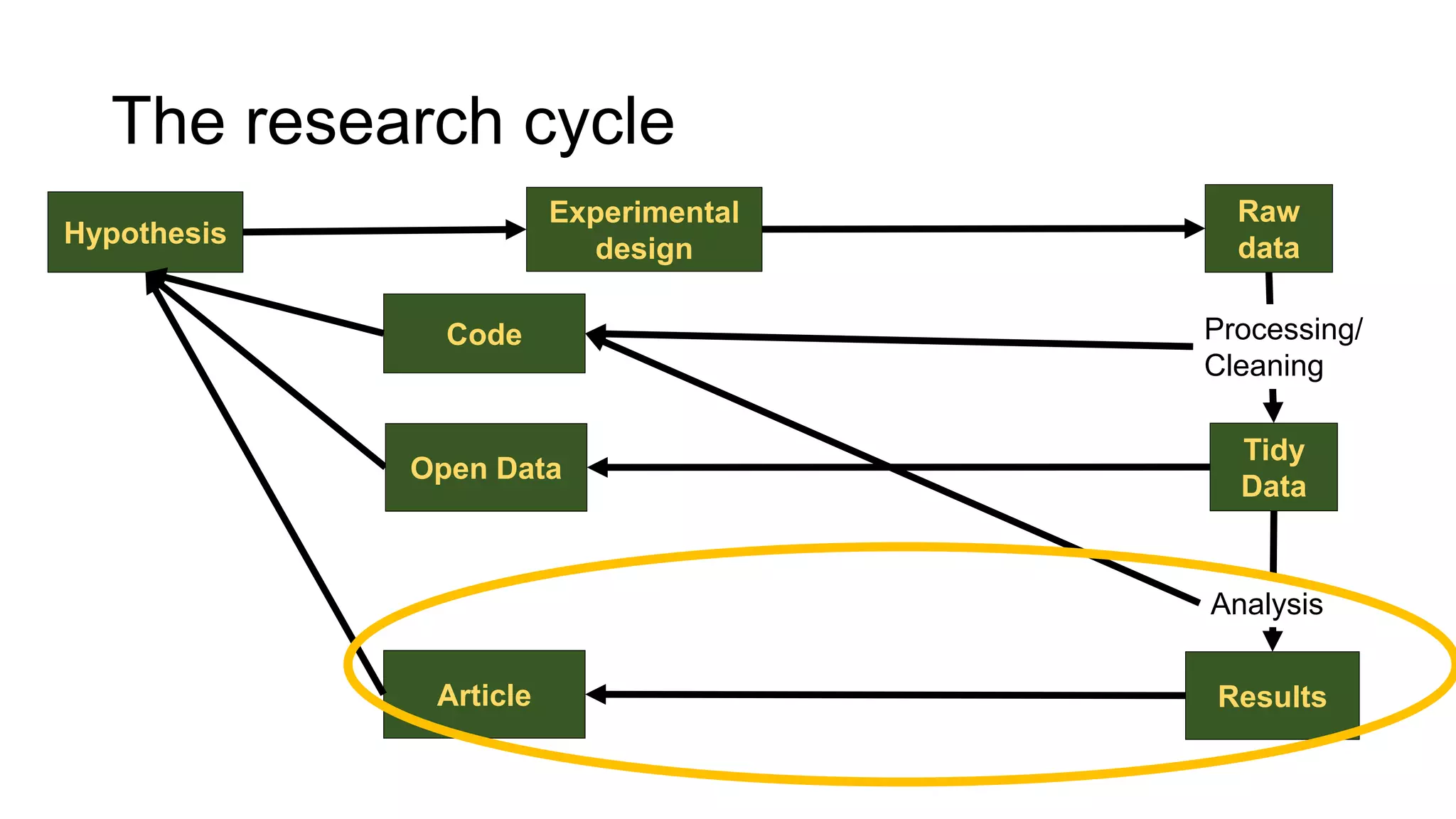
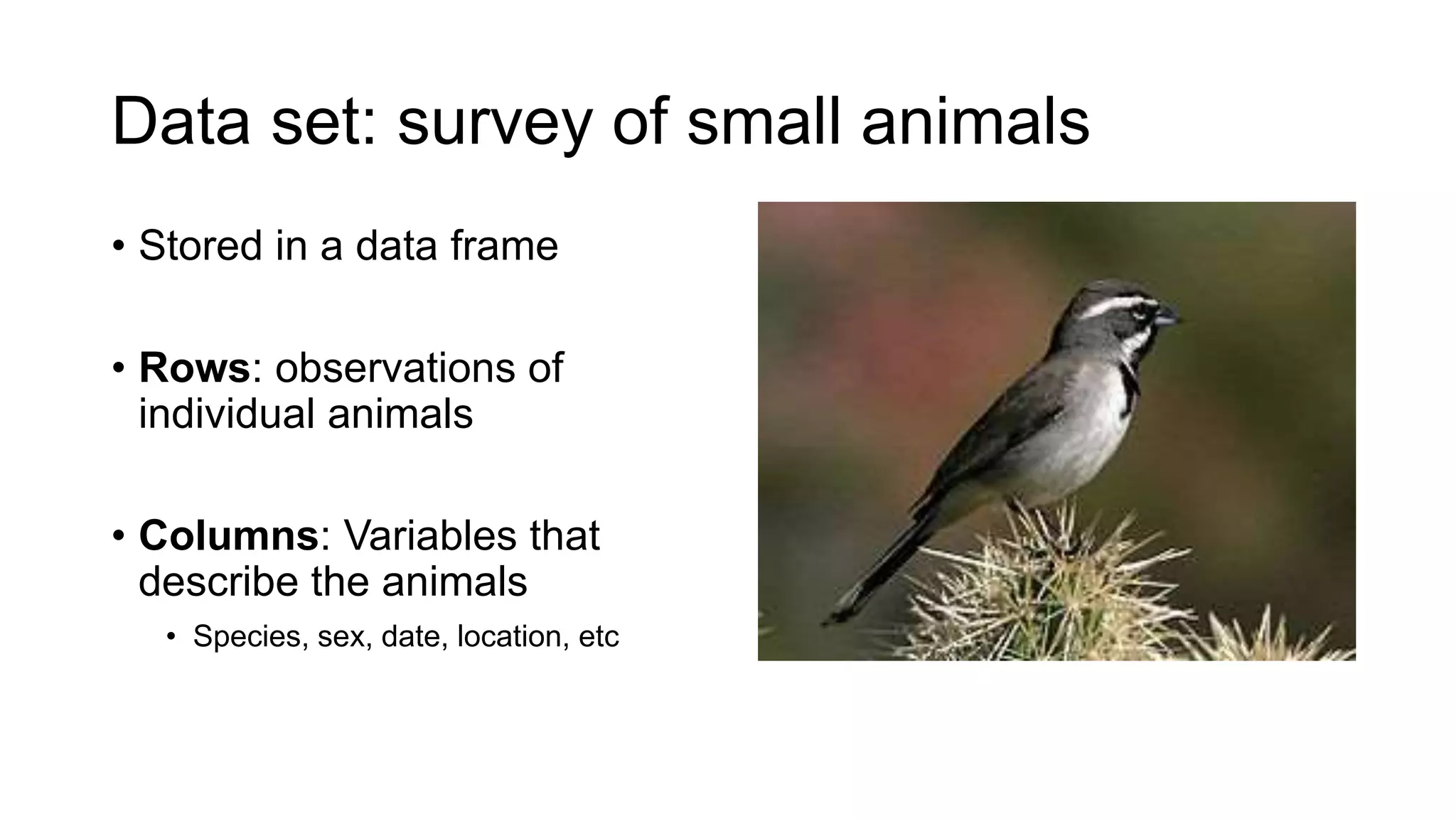
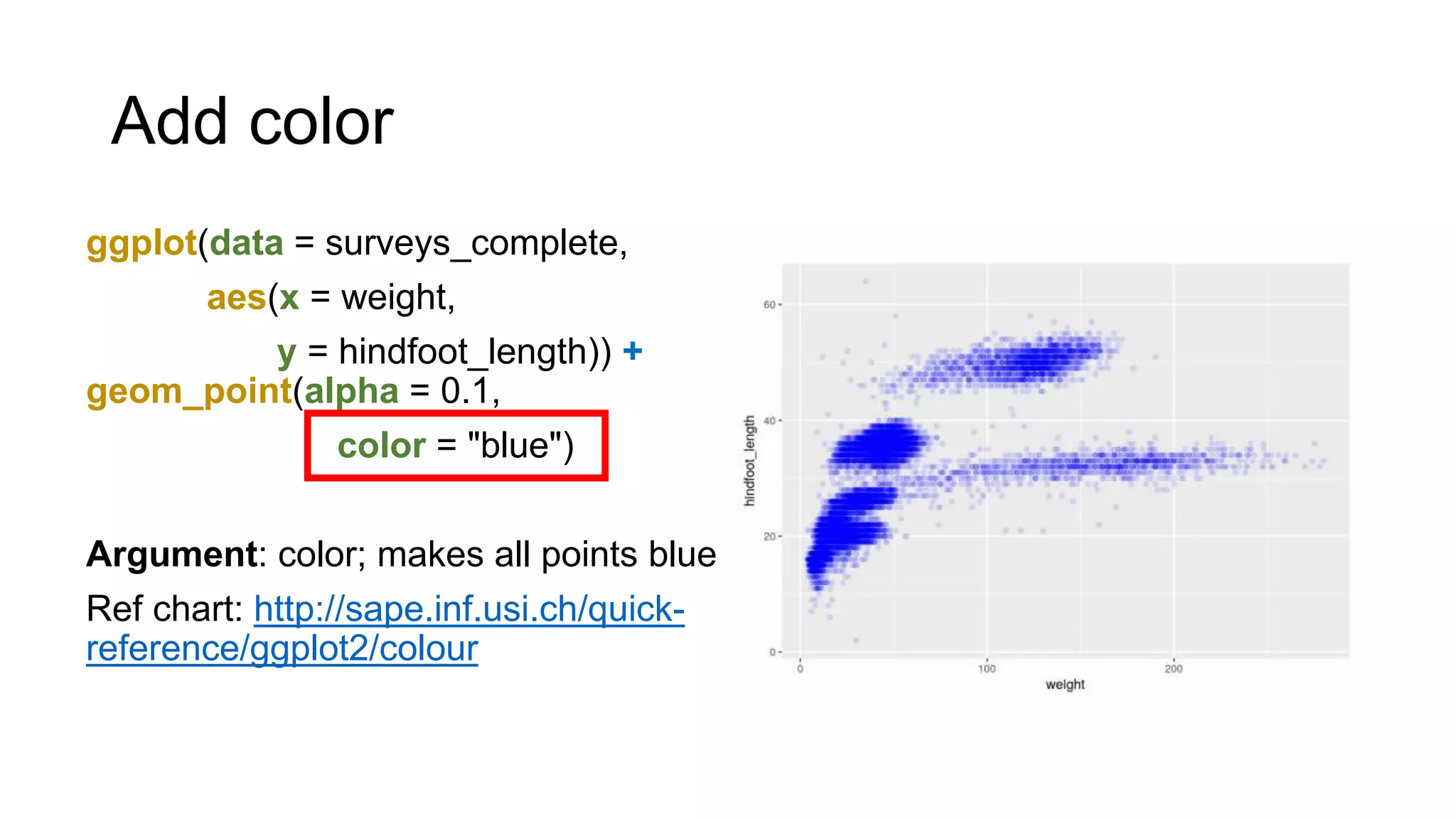
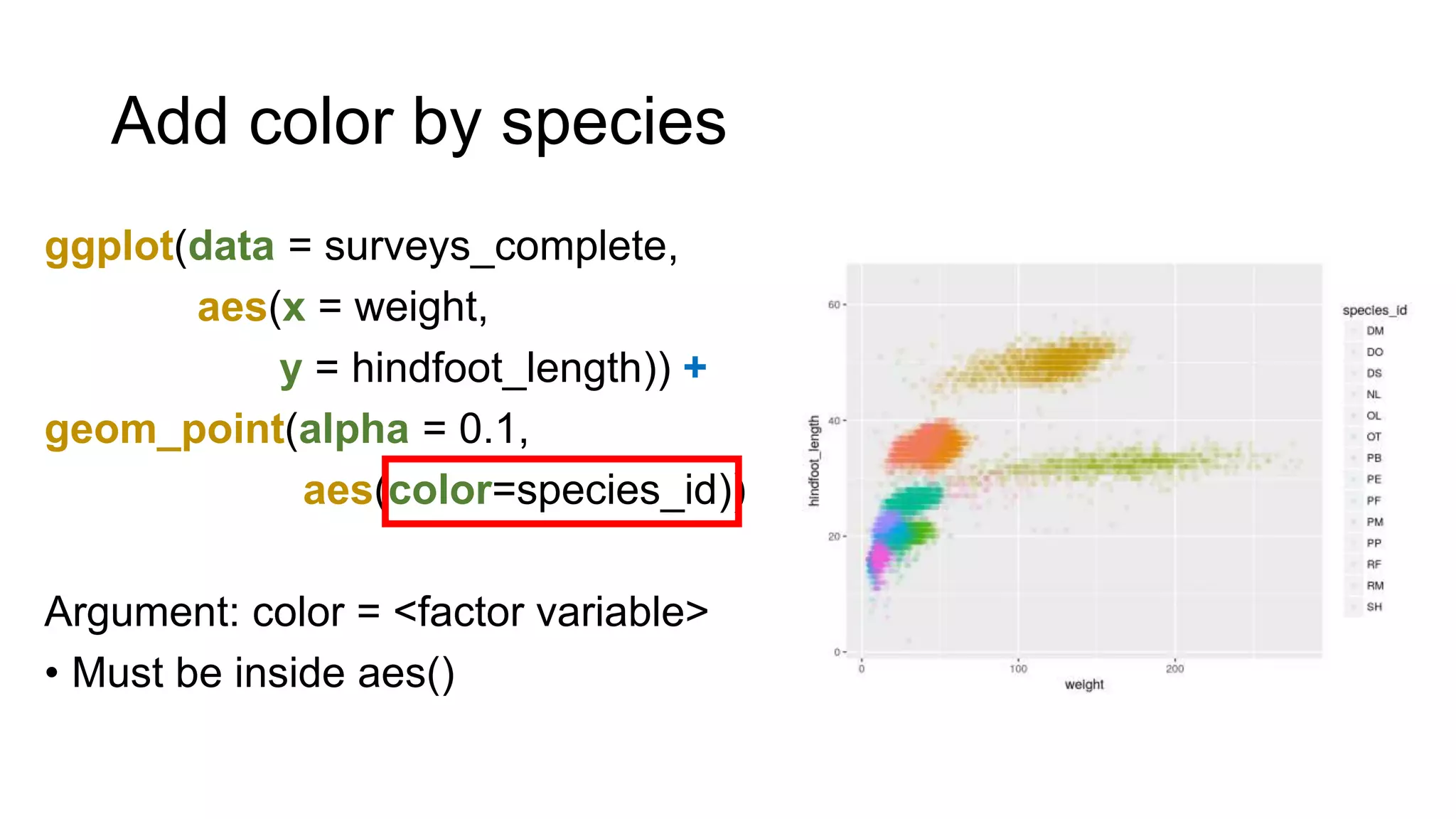
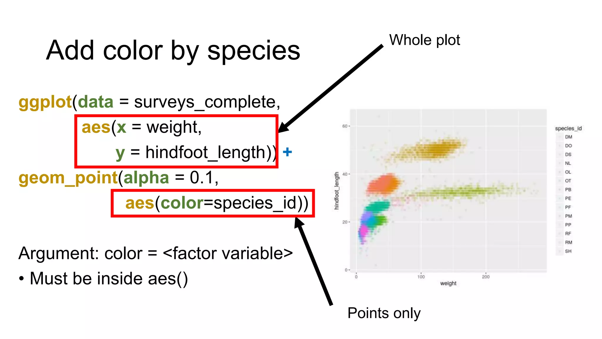
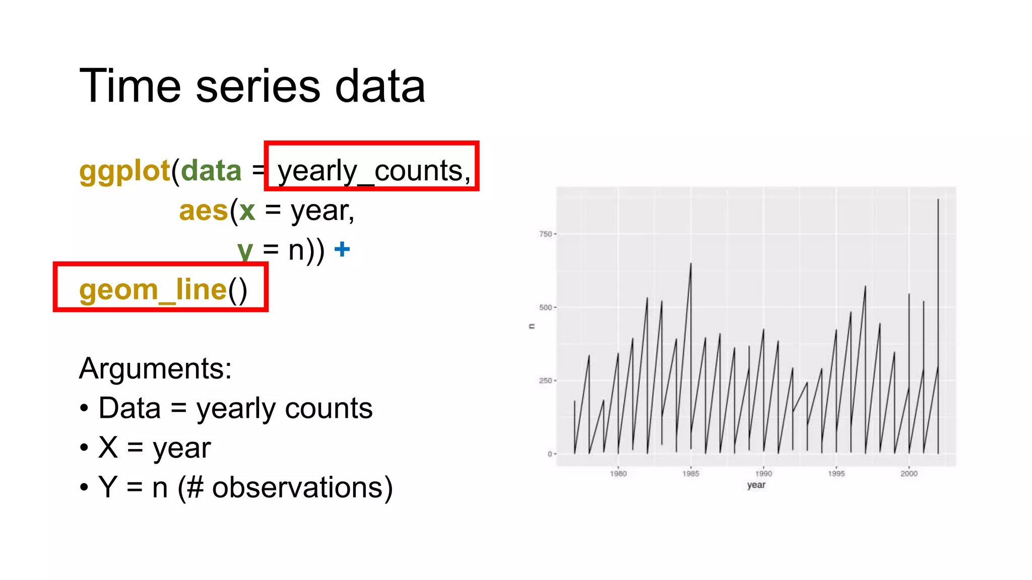
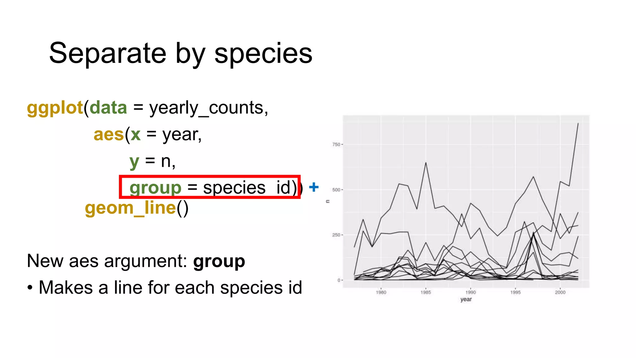
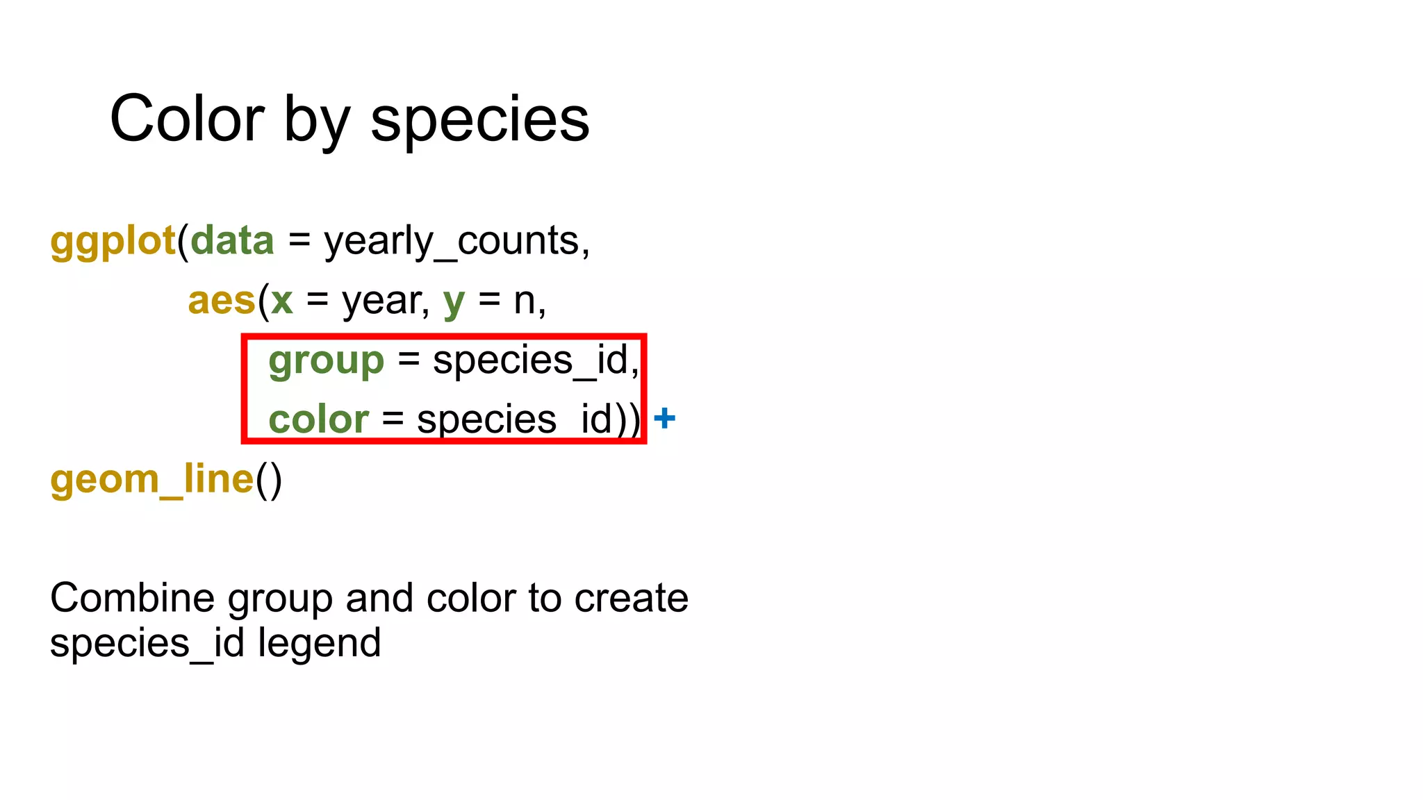
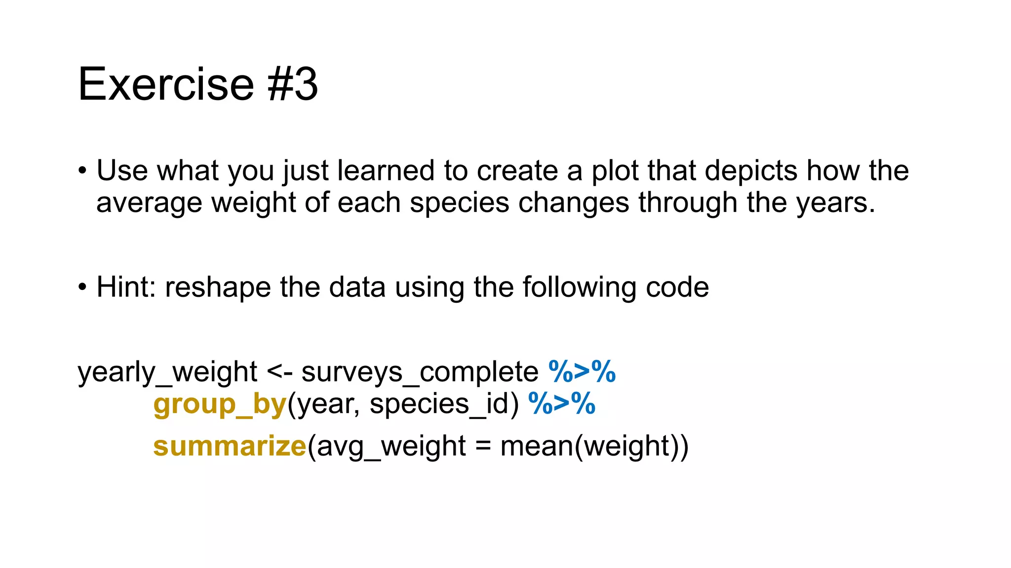
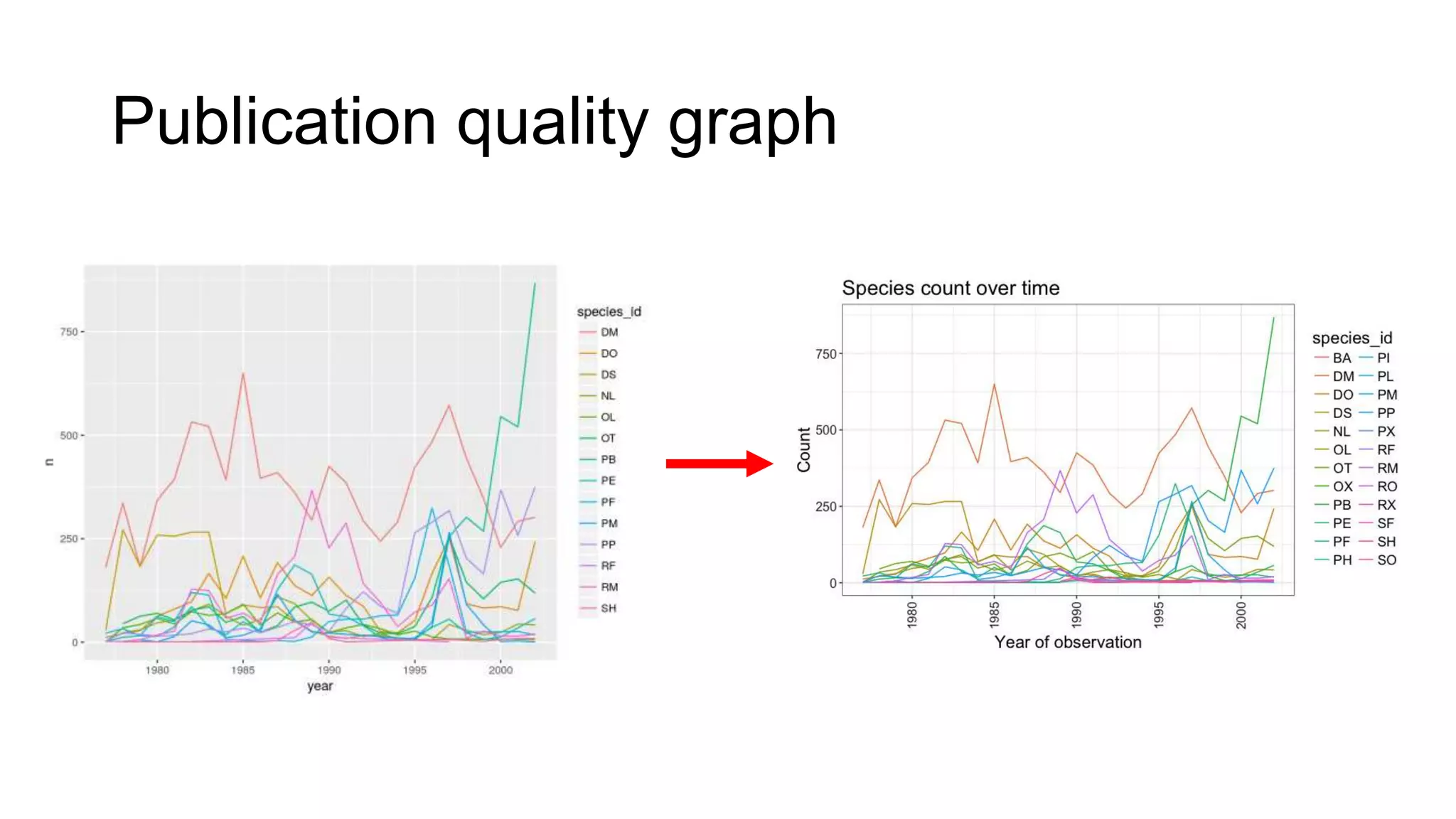
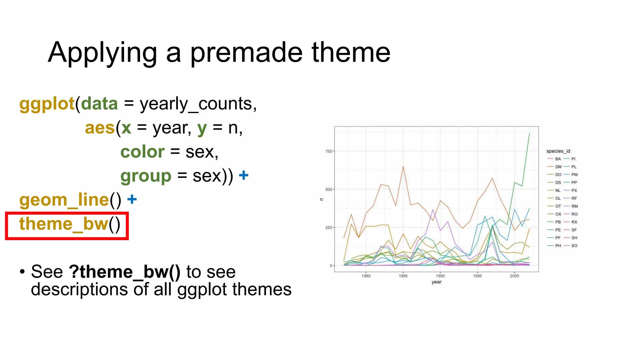
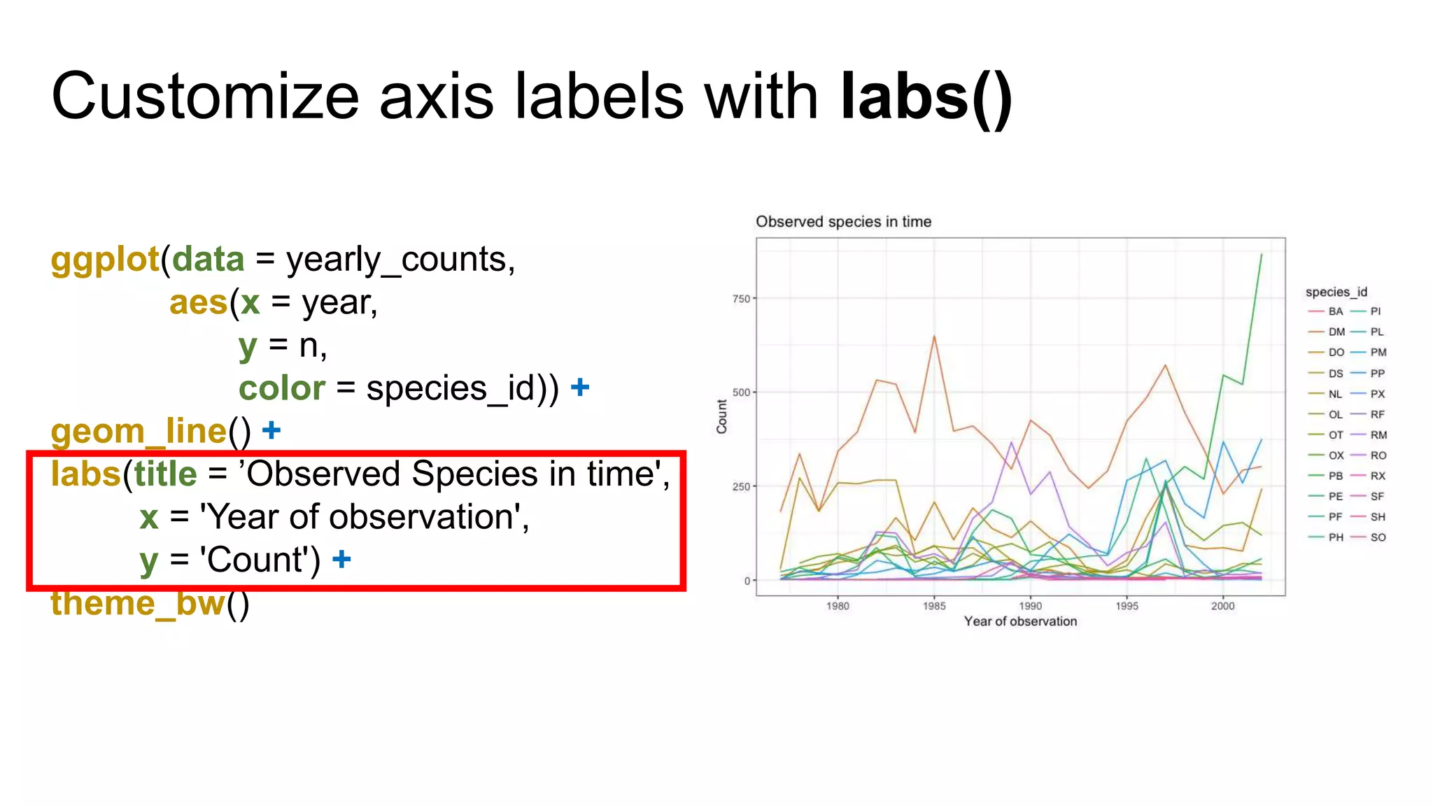
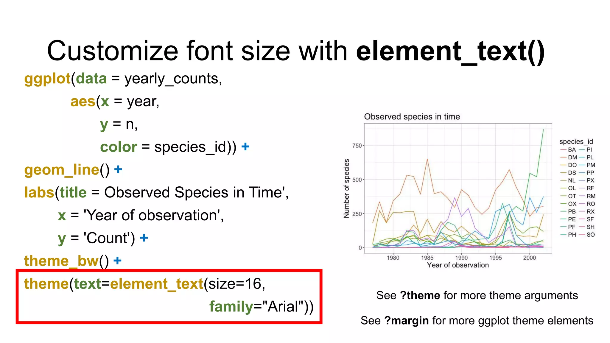
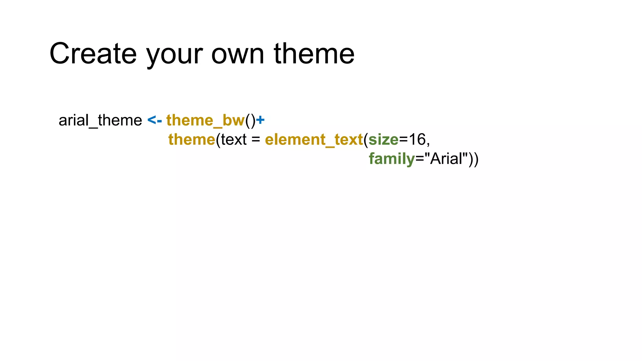
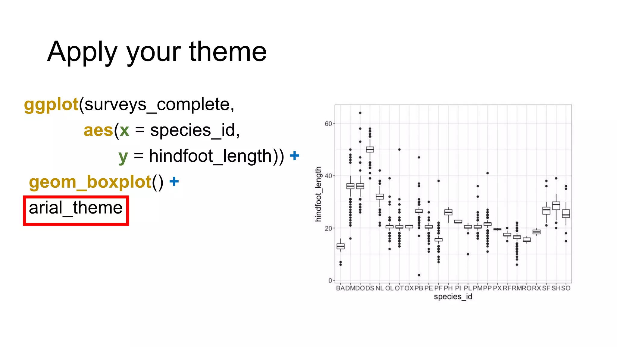
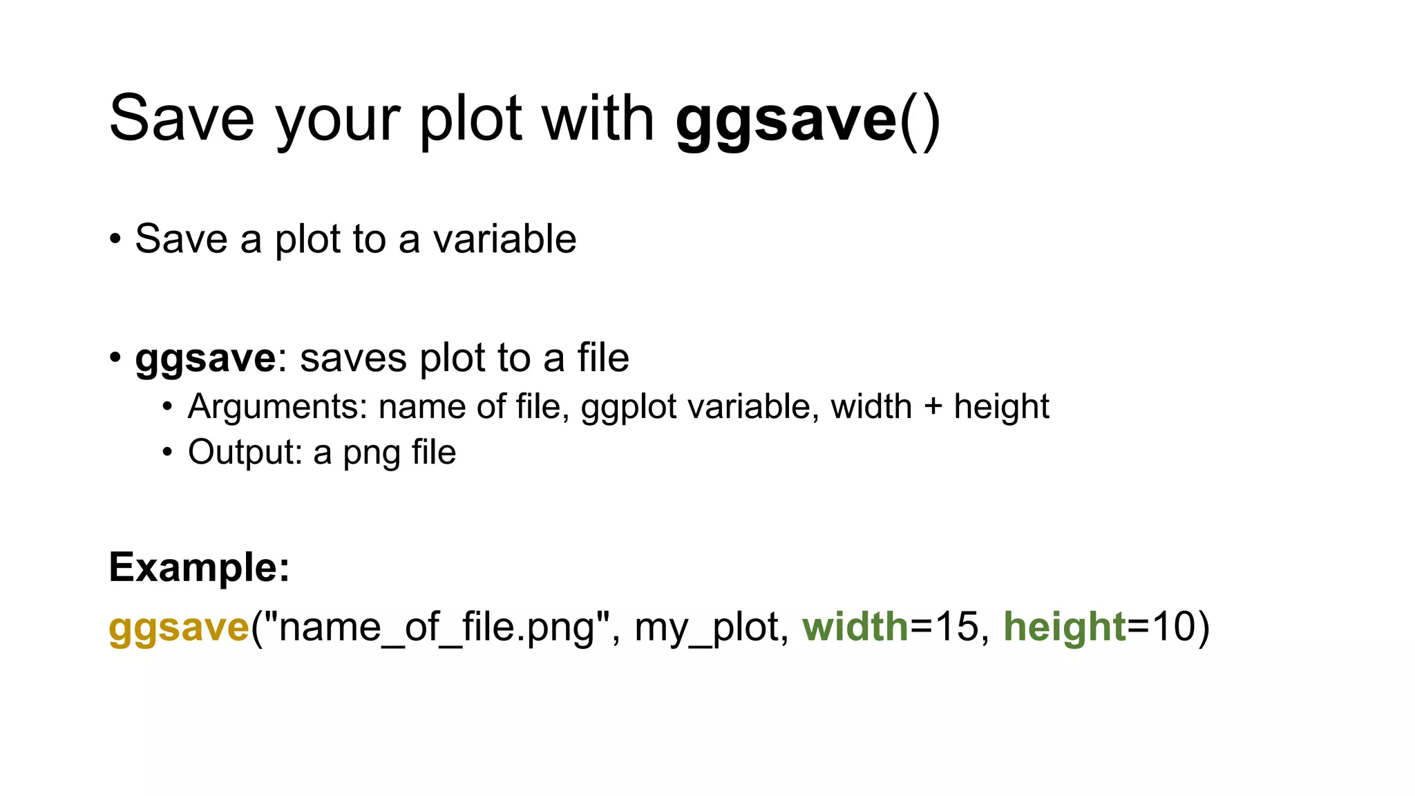
Data Visualization
using R
C. Tobin Magle, PhD
05-16-2017
10:00-11:30 a.m.
Morgan Library
Computer Classroom 175
Based on http://www.datacarpentry.org/R-ecology-lesson/
Hypothesis
Raw
data
Experimental
design
Tidy
Data
ResultsArticle
Processing/
Cleaning
Analysis
Open Data
Code
The research cycle
Outline
• Basic elements (data, aesthetics, geoms)
• Modifications (transparency, color, grouping)
• Themes (modifying default, using premade, saving your own)
• Exporting plots (ggsave)
Setup
• Install R and R studio
http://www.datacarpentry.org/R-ecology-lesson/index.html#setup_instructions
• Download the quickstart files: http://tinyurl.com/kp6bxt4
• See the Basic Analysis with R lesson if you’re unfamiliar with R
or R studio
http://libguides.colostate.edu/data-and-donuts/r-analysis
Data set: survey of small animals
• Stored in a data frame
• Rows: observations of
individual animals
• Columns: Variables that
describe the animals
• Species, sex, date, location, etc
Load data into R
• Import data using read.csv function
• Arguments: a csv file
• Output: a data frame
Example: surveys <- read.csv('data/surveys_complete.csv')
Graphics with ggplot2
• data: data frame
• aesthetics: looks
• geoms: type of plot
• Ex: points, lines, bars
ggplot2 functions
• ggplot(): initializes ggplot object
• aes(): draws axes based on arguments
• geom_XXX(): draws points/lines etc.
• + operator: adds components to plot
• Modular structure
Simplest ggplot
Need data, aesthetics and a geom
to create a plot.
Example:
ggplot(data = surveys_complete,
aes(x = weight,
y = hindfoot_length)) +
geom_point()
ggplot()
ggplot(data = surveys_complete)
Argument: data frame
Output: blank plot area
ggplot() + aes()
ggplot(data = surveys_complete,
aes(x = weight,
y = hindfoot_length))
ggplot arguments:
data frame + aes()
aes arguments:
• x = x axis variable
• y = y axis variable
• Output: draws axes
ggplot + aes + geom_point
ggplot(data = surveys_complete,
aes(x = weight,
y = hindfoot_length)) +
geom_point()
+ operator: adds point to the
specified plot area
Output: scatterplot of weigh vs.
hindfood length
Add transparency
ggplot(data = surveys_complete,
aes(x = weight,
y = hindfoot_length)) +
geom_point(alpha = 0.1)
Argument: alpha = 0.1
• 1/10 opacity
• Range: 0-1
Add color
ggplot(data = surveys_complete,
aes(x = weight,
y = hindfoot_length)) +
geom_point(alpha = 0.1,
color = "blue")
Argument: color; makes all points blue
Ref chart: http://sape.inf.usi.ch/quick-
reference/ggplot2/colour
Add color by species
ggplot(data = surveys_complete,
aes(x = weight,
y = hindfoot_length)) +
geom_point(alpha = 0.1,
aes(color=species_id))
Argument: color = <factor variable>
• Must be inside aes()
Add color by species
ggplot(data = surveys_complete,
aes(x = weight,
y = hindfoot_length)) +
geom_point(alpha = 0.1,
aes(color=species_id))
Argument: color = <factor variable>
• Must be inside aes()
Points only
Whole plot
Exercise 1
• Use the previous example as a starting point.
• Add color to the data points according to the plot from which the
sample was taken (plot_id).
• Hint: Check the class for plot_id. Consider changing the class
of plot_id from integer to factor. Why does this change how R
makes the graph?
Plot factor variables with box plot
ggplot(data = surveys_complete,
aes(x = species_id,
y = hindfoot_length)) +
geom_boxplot()
aes arguments:
• x: species id (factor)
• y: hinfoot length (numeric)
Overlay points on a box plot
ggplot(data = surveys_complete,
aes(x = species_id,
y = hindfoot_length)) +
geom_boxplot(alpha = 0) +
geom_jitter(alpha = 0.3,
color = "tomato")
Exercise 2: Violin plot
• Plot the same data as in the previous example, but as a Violin
plot
• Hint: see geom_violin().
• What information does this give you about the data that a box
plot does?
Time series data
Reshape data:
yearly_counts <- surveys_complete %>%
group_by(year, species_id) %>%
tally
Time series data
ggplot(data = yearly_counts,
aes(x = year,
y = n)) +
geom_line()
Arguments:
• Data = yearly counts
• X = year
• Y = n (# observations)
Separate by species
ggplot(data = yearly_counts,
aes(x = year,
y = n,
group = species_id)) +
geom_line()
New aes argument: group
• Makes a line for each species id
Color by species
ggplot(data = yearly_counts,
aes(x = year, y = n,
group = species_id,
color = species_id)) +
geom_line()
Combine group and color to create
species_id legend
Exercise #3
• Use what you just learned to create a plot that depicts how the
average weight of each species changes through the years.
• Hint: reshape the data using the following code
yearly_weight <- surveys_complete %>%
group_by(year, species_id) %>%
summarize(avg_weight = mean(weight))
Publication quality graph
Applying a premade theme
ggplot(data = yearly_counts,
aes(x = year, y = n,
color = sex,
group = sex)) +
geom_line() +
theme_bw()
• See ?theme_bw() to see
descriptions of all ggplot themes
Customize axis labels with labs()
ggplot(data = yearly_counts,
aes(x = year,
y = n,
color = species_id)) +
geom_line() +
labs(title = ’Observed Species in time',
x = 'Year of observation',
y = 'Count') +
theme_bw()
Customize font size with element_text()
ggplot(data = yearly_counts,
aes(x = year,
y = n,
color = species_id)) +
geom_line() +
labs(title = Observed Species in Time',
x = 'Year of observation',
y = 'Count') +
theme_bw() +
theme(text=element_text(size=16,
family="Arial"))
See ?margin for more ggplot theme elements
See ?theme for more theme arguments
Create your own theme
arial_theme <- theme_bw()+
theme(text = element_text(size=16,
family="Arial"))
Apply your theme
ggplot(surveys_complete,
aes(x = species_id,
y = hindfoot_length)) +
geom_boxplot() +
arial_theme
Save your plot with ggsave()
• Save a plot to a variable
• ggsave: saves plot to a file
• Arguments: name of file, ggplot variable, width + height
• Output: a png file
Example:
ggsave("name_of_file.png", my_plot, width=15, height=10)
Need help?
• Email: tobin.magle@colostate.edu
• Data Management Services website:
http://lib.colostate.edu/services/data-management
• Data Carpentry: http://www.datacarpentry.org/
• R Ecology Lesson:
http://www.datacarpentry.org/R-ecology-lesson/04-visualization-ggplot2.html
• Ggplot2 Cheat Sheets:
• https://www.rstudio.com/wp-content/uploads/2015/03/ggplot2-cheatsheet.pdf

Data and donuts: Data Visualization using R

  • 1.
    Data Visualization using R C.Tobin Magle, PhD 05-16-2017 10:00-11:30 a.m. Morgan Library Computer Classroom 175 Based on http://www.datacarpentry.org/R-ecology-lesson/
  • 2.
  • 3.
    Outline • Basic elements(data, aesthetics, geoms) • Modifications (transparency, color, grouping) • Themes (modifying default, using premade, saving your own) • Exporting plots (ggsave)
  • 4.
    Setup • Install Rand R studio http://www.datacarpentry.org/R-ecology-lesson/index.html#setup_instructions • Download the quickstart files: http://tinyurl.com/kp6bxt4 • See the Basic Analysis with R lesson if you’re unfamiliar with R or R studio http://libguides.colostate.edu/data-and-donuts/r-analysis
  • 5.
    Data set: surveyof small animals • Stored in a data frame • Rows: observations of individual animals • Columns: Variables that describe the animals • Species, sex, date, location, etc
  • 6.
    Load data intoR • Import data using read.csv function • Arguments: a csv file • Output: a data frame Example: surveys <- read.csv('data/surveys_complete.csv')
  • 7.
    Graphics with ggplot2 •data: data frame • aesthetics: looks • geoms: type of plot • Ex: points, lines, bars
  • 8.
    ggplot2 functions • ggplot():initializes ggplot object • aes(): draws axes based on arguments • geom_XXX(): draws points/lines etc. • + operator: adds components to plot • Modular structure
  • 9.
    Simplest ggplot Need data,aesthetics and a geom to create a plot. Example: ggplot(data = surveys_complete, aes(x = weight, y = hindfoot_length)) + geom_point()
  • 10.
    ggplot() ggplot(data = surveys_complete) Argument:data frame Output: blank plot area
  • 11.
    ggplot() + aes() ggplot(data= surveys_complete, aes(x = weight, y = hindfoot_length)) ggplot arguments: data frame + aes() aes arguments: • x = x axis variable • y = y axis variable • Output: draws axes
  • 12.
    ggplot + aes+ geom_point ggplot(data = surveys_complete, aes(x = weight, y = hindfoot_length)) + geom_point() + operator: adds point to the specified plot area Output: scatterplot of weigh vs. hindfood length
  • 13.
    Add transparency ggplot(data =surveys_complete, aes(x = weight, y = hindfoot_length)) + geom_point(alpha = 0.1) Argument: alpha = 0.1 • 1/10 opacity • Range: 0-1
  • 14.
    Add color ggplot(data =surveys_complete, aes(x = weight, y = hindfoot_length)) + geom_point(alpha = 0.1, color = "blue") Argument: color; makes all points blue Ref chart: http://sape.inf.usi.ch/quick- reference/ggplot2/colour
  • 15.
    Add color byspecies ggplot(data = surveys_complete, aes(x = weight, y = hindfoot_length)) + geom_point(alpha = 0.1, aes(color=species_id)) Argument: color = <factor variable> • Must be inside aes()
  • 16.
    Add color byspecies ggplot(data = surveys_complete, aes(x = weight, y = hindfoot_length)) + geom_point(alpha = 0.1, aes(color=species_id)) Argument: color = <factor variable> • Must be inside aes() Points only Whole plot
  • 17.
    Exercise 1 • Usethe previous example as a starting point. • Add color to the data points according to the plot from which the sample was taken (plot_id). • Hint: Check the class for plot_id. Consider changing the class of plot_id from integer to factor. Why does this change how R makes the graph?
  • 18.
    Plot factor variableswith box plot ggplot(data = surveys_complete, aes(x = species_id, y = hindfoot_length)) + geom_boxplot() aes arguments: • x: species id (factor) • y: hinfoot length (numeric)
  • 19.
    Overlay points ona box plot ggplot(data = surveys_complete, aes(x = species_id, y = hindfoot_length)) + geom_boxplot(alpha = 0) + geom_jitter(alpha = 0.3, color = "tomato")
  • 20.
    Exercise 2: Violinplot • Plot the same data as in the previous example, but as a Violin plot • Hint: see geom_violin(). • What information does this give you about the data that a box plot does?
  • 21.
    Time series data Reshapedata: yearly_counts <- surveys_complete %>% group_by(year, species_id) %>% tally
  • 22.
    Time series data ggplot(data= yearly_counts, aes(x = year, y = n)) + geom_line() Arguments: • Data = yearly counts • X = year • Y = n (# observations)
  • 23.
    Separate by species ggplot(data= yearly_counts, aes(x = year, y = n, group = species_id)) + geom_line() New aes argument: group • Makes a line for each species id
  • 24.
    Color by species ggplot(data= yearly_counts, aes(x = year, y = n, group = species_id, color = species_id)) + geom_line() Combine group and color to create species_id legend
  • 25.
    Exercise #3 • Usewhat you just learned to create a plot that depicts how the average weight of each species changes through the years. • Hint: reshape the data using the following code yearly_weight <- surveys_complete %>% group_by(year, species_id) %>% summarize(avg_weight = mean(weight))
  • 26.
  • 27.
    Applying a premadetheme ggplot(data = yearly_counts, aes(x = year, y = n, color = sex, group = sex)) + geom_line() + theme_bw() • See ?theme_bw() to see descriptions of all ggplot themes
  • 28.
    Customize axis labelswith labs() ggplot(data = yearly_counts, aes(x = year, y = n, color = species_id)) + geom_line() + labs(title = ’Observed Species in time', x = 'Year of observation', y = 'Count') + theme_bw()
  • 29.
    Customize font sizewith element_text() ggplot(data = yearly_counts, aes(x = year, y = n, color = species_id)) + geom_line() + labs(title = Observed Species in Time', x = 'Year of observation', y = 'Count') + theme_bw() + theme(text=element_text(size=16, family="Arial")) See ?margin for more ggplot theme elements See ?theme for more theme arguments
  • 30.
    Create your owntheme arial_theme <- theme_bw()+ theme(text = element_text(size=16, family="Arial"))
  • 31.
    Apply your theme ggplot(surveys_complete, aes(x= species_id, y = hindfoot_length)) + geom_boxplot() + arial_theme
  • 32.
    Save your plotwith ggsave() • Save a plot to a variable • ggsave: saves plot to a file • Arguments: name of file, ggplot variable, width + height • Output: a png file Example: ggsave("name_of_file.png", my_plot, width=15, height=10)
  • 33.
    Need help? • Email:tobin.magle@colostate.edu • Data Management Services website: http://lib.colostate.edu/services/data-management • Data Carpentry: http://www.datacarpentry.org/ • R Ecology Lesson: http://www.datacarpentry.org/R-ecology-lesson/04-visualization-ggplot2.html • Ggplot2 Cheat Sheets: • https://www.rstudio.com/wp-content/uploads/2015/03/ggplot2-cheatsheet.pdf