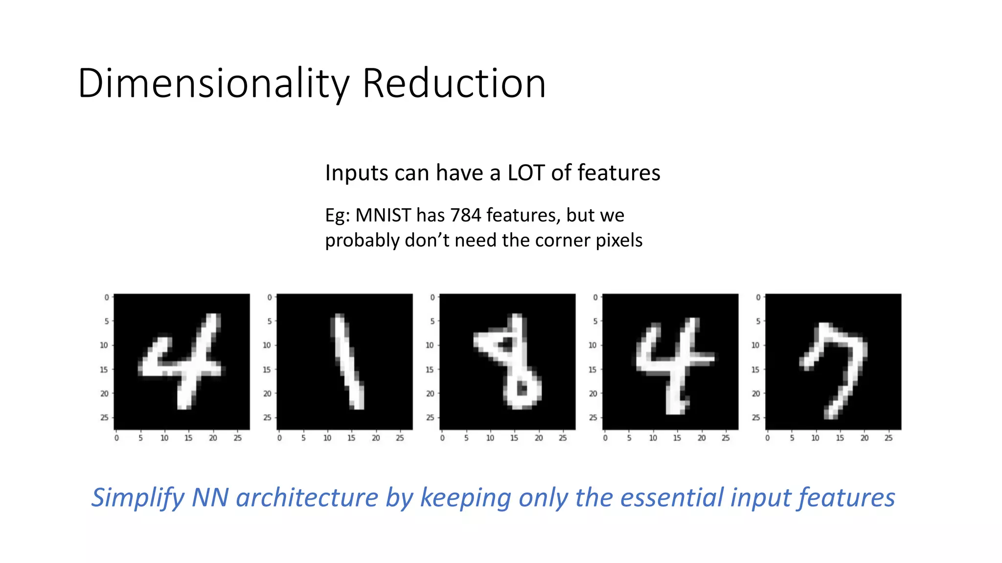
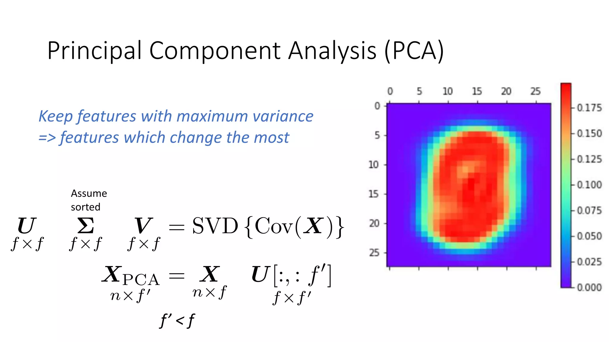
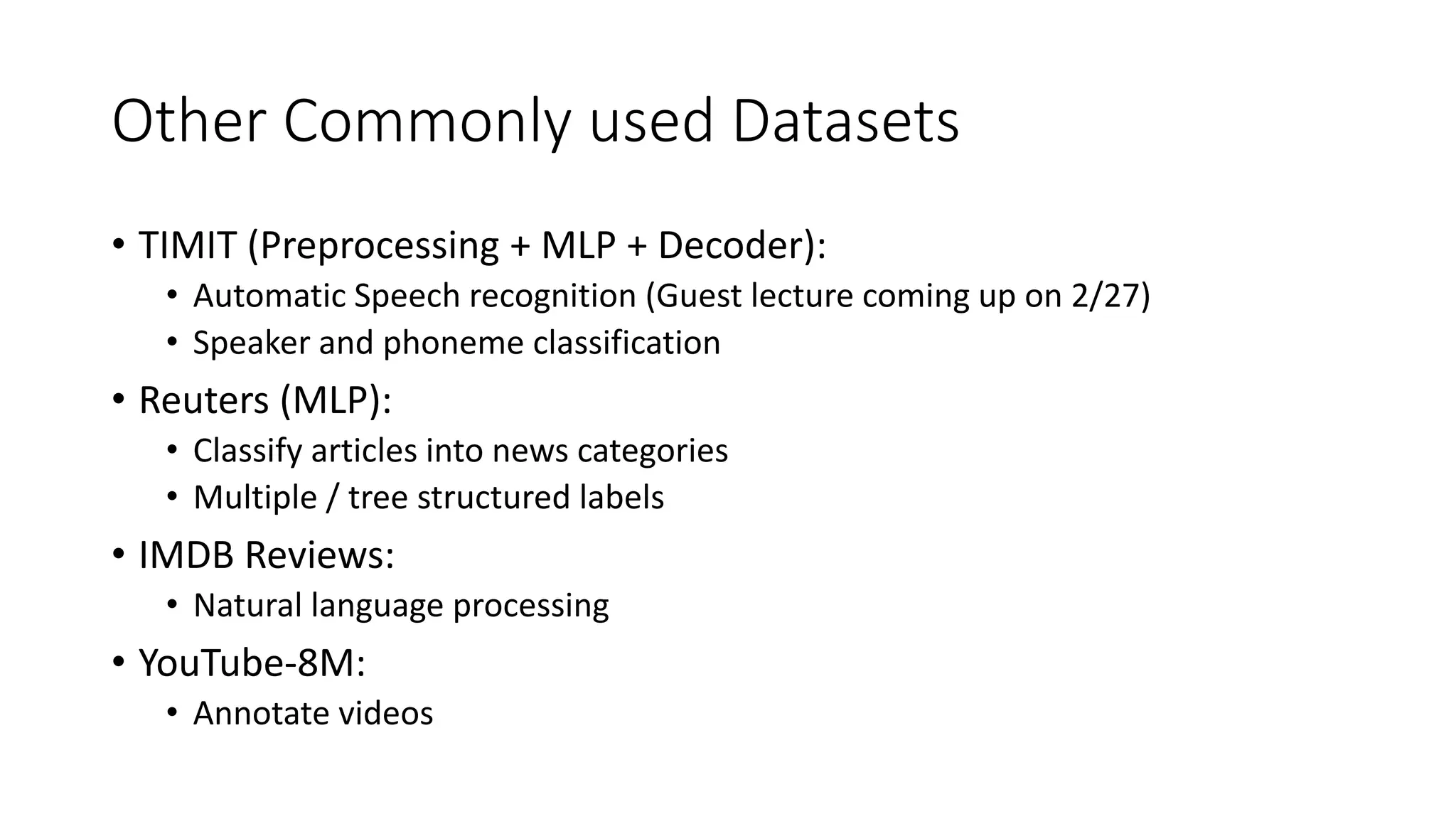
Downloaded 19 times

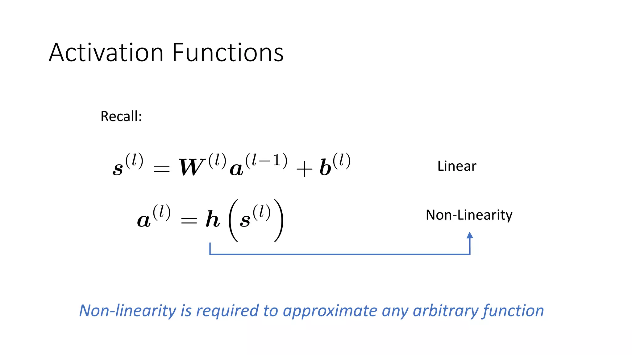
![ReLU family of activations
x >= 0 x < 0
Rectified Linear Unit (ReLU) x 0
Exponential Linear Unit (ELU) x α(ex - 1)
Leaky ReLU x αx
Biologically inspired - neurons firing vs not firing
Solves vanishing gradient problem
Non-differentiable at 0, replace with anything in [0,1]
ReLU can die if x<0
Leaky ReLU solves this, but inconsistent results
ELU saturates for x<0, so less resistant to noise
Clevert, Djork-Arné; Unterthiner, Thomas; Hochreiter, Sepp (2015-11-23). "Fast and
Accurate Deep Network Learning by Exponential Linear Units (ELUs)". arXiv:1511.07289](https://image.slidesharecdn.com/techniquesdeeplearning-191231140206/75/Techniques-in-Deep-Learning-8-2048.jpg)

![Comparison of Initializers
Weights
initialized
with all 0s
Weights
stay as
all 0s !!
Histograms of a few weights in 2nd
junction after training for 10 epochs
MNIST [784,200,10]
Regularization: None](https://image.slidesharecdn.com/techniquesdeeplearning-191231140206/75/Techniques-in-Deep-Learning-75-2048.jpg)
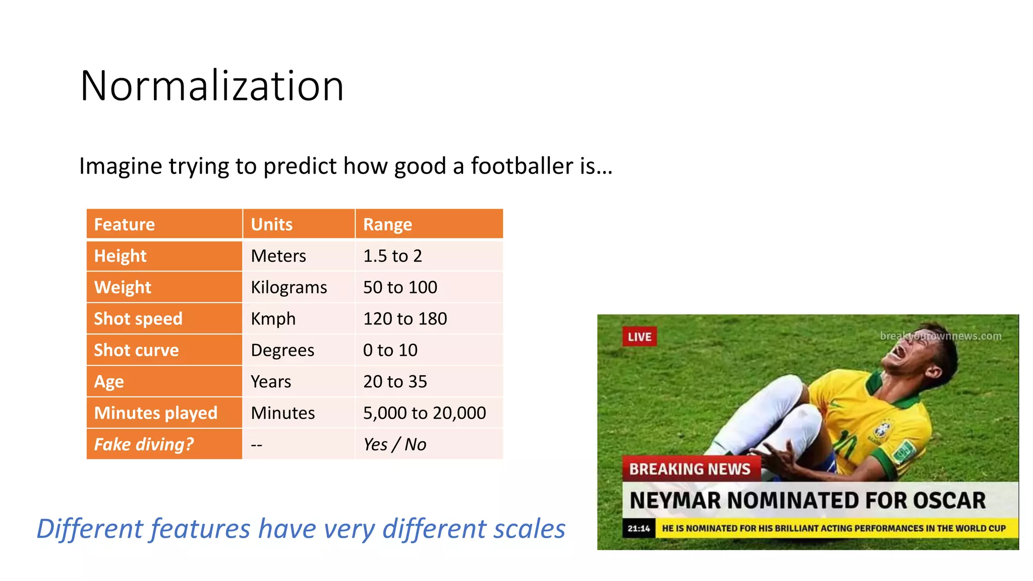
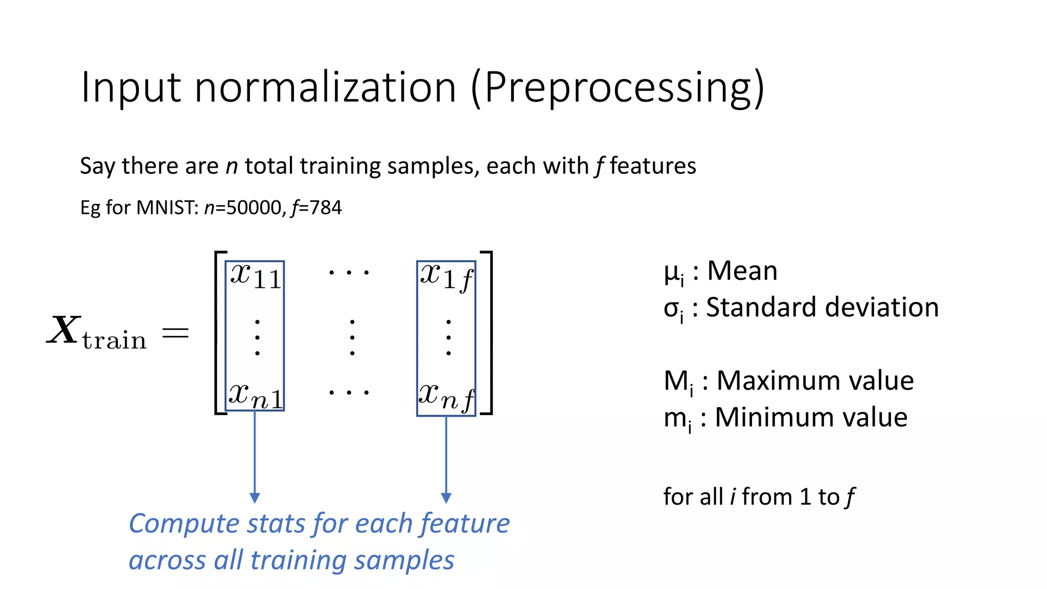
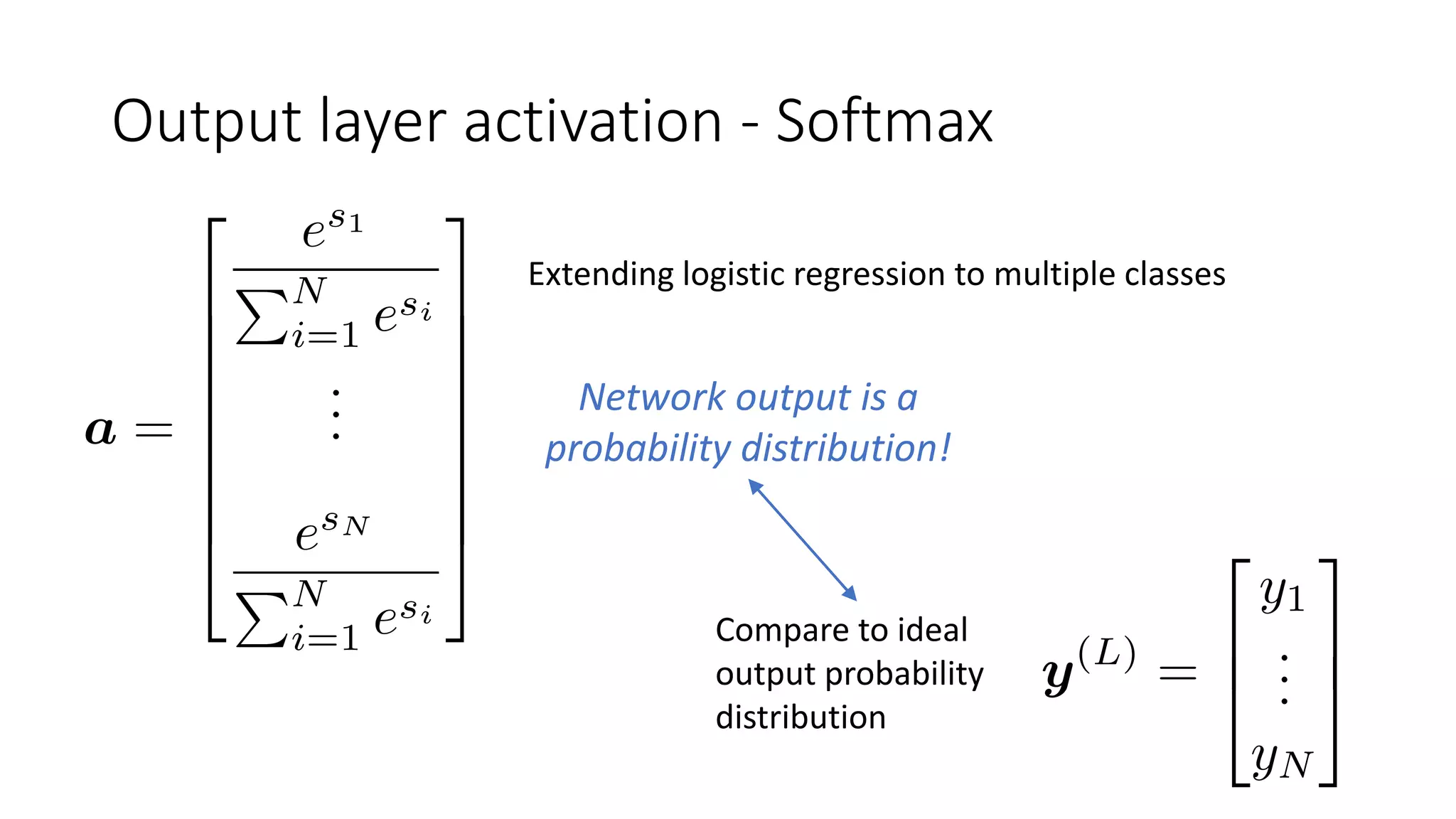
![Essential preprocessing
Gaussian normalization:
Each feature is a unit Gaussian
Minmax normalization:
Each feature is in [0,1]](https://image.slidesharecdn.com/techniquesdeeplearning-191231140206/75/Techniques-in-Deep-Learning-79-2048.jpg)


![ReLU family of activations
x >= 0 x < 0
Rectified Linear Unit (ReLU) x 0
Exponential Linear Unit (ELU) x α(ex - 1)
Leaky ReLU x αx
Biologically inspired - neurons firing vs not firing
Solves vanishing gradient problem
Non-differentiable at 0, replace with anything in [0,1]
ReLU can die if x<0
Leaky ReLU solves this, but inconsistent results
ELU saturates for x<0, so less resistant to noise
Clevert, Djork-Arné; Unterthiner, Thomas; Hochreiter, Sepp (2015-11-23). "Fast and
Accurate Deep Network Learning by Exponential Linear Units (ELUs)". arXiv:1511.07289](https://crownmelresort.com/image.slidesharecdn.com/techniquesdeeplearning-191231140206/75/Techniques-in-Deep-Learning-8-2048.jpg)


![Comparison of Initializers
Weights
initialized
with all 0s
Weights
stay as
all 0s !!
Histograms of a few weights in 2nd
junction after training for 10 epochs
MNIST [784,200,10]
Regularization: None](https://crownmelresort.com/image.slidesharecdn.com/techniquesdeeplearning-191231140206/75/Techniques-in-Deep-Learning-75-2048.jpg)


![Essential preprocessing
Gaussian normalization:
Each feature is a unit Gaussian
Minmax normalization:
Each feature is in [0,1]](https://crownmelresort.com/image.slidesharecdn.com/techniquesdeeplearning-191231140206/75/Techniques-in-Deep-Learning-79-2048.jpg)


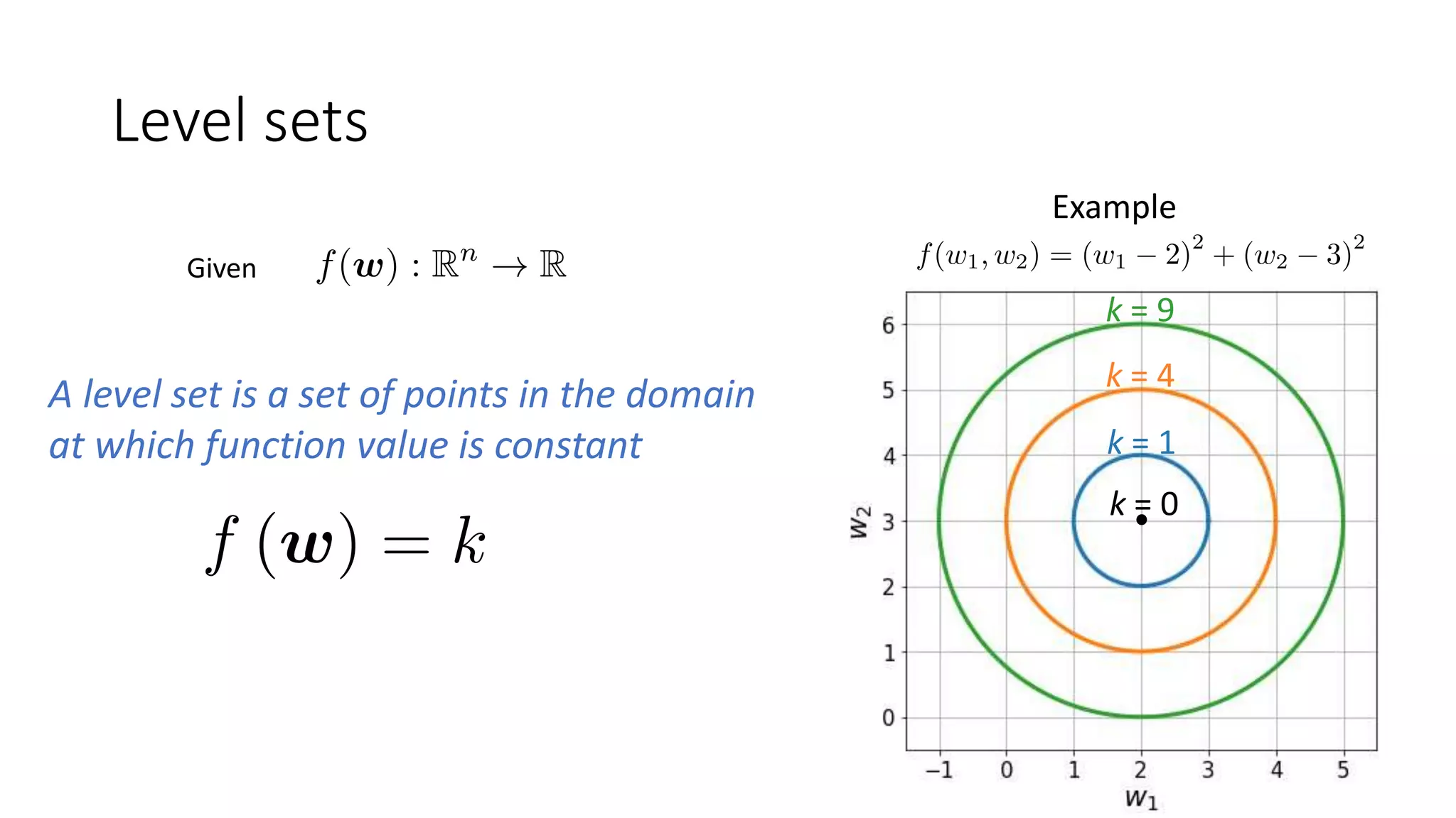
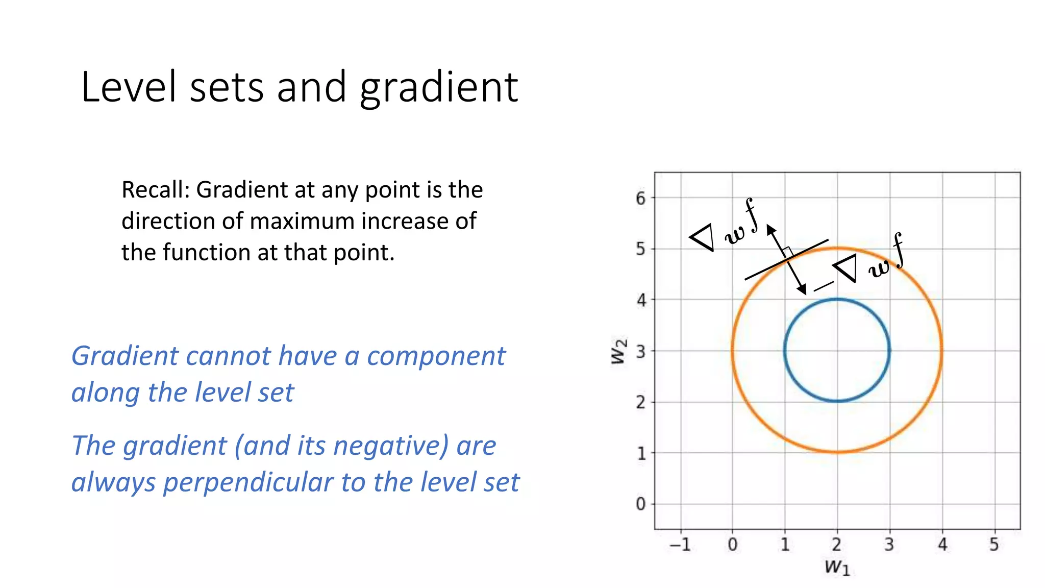
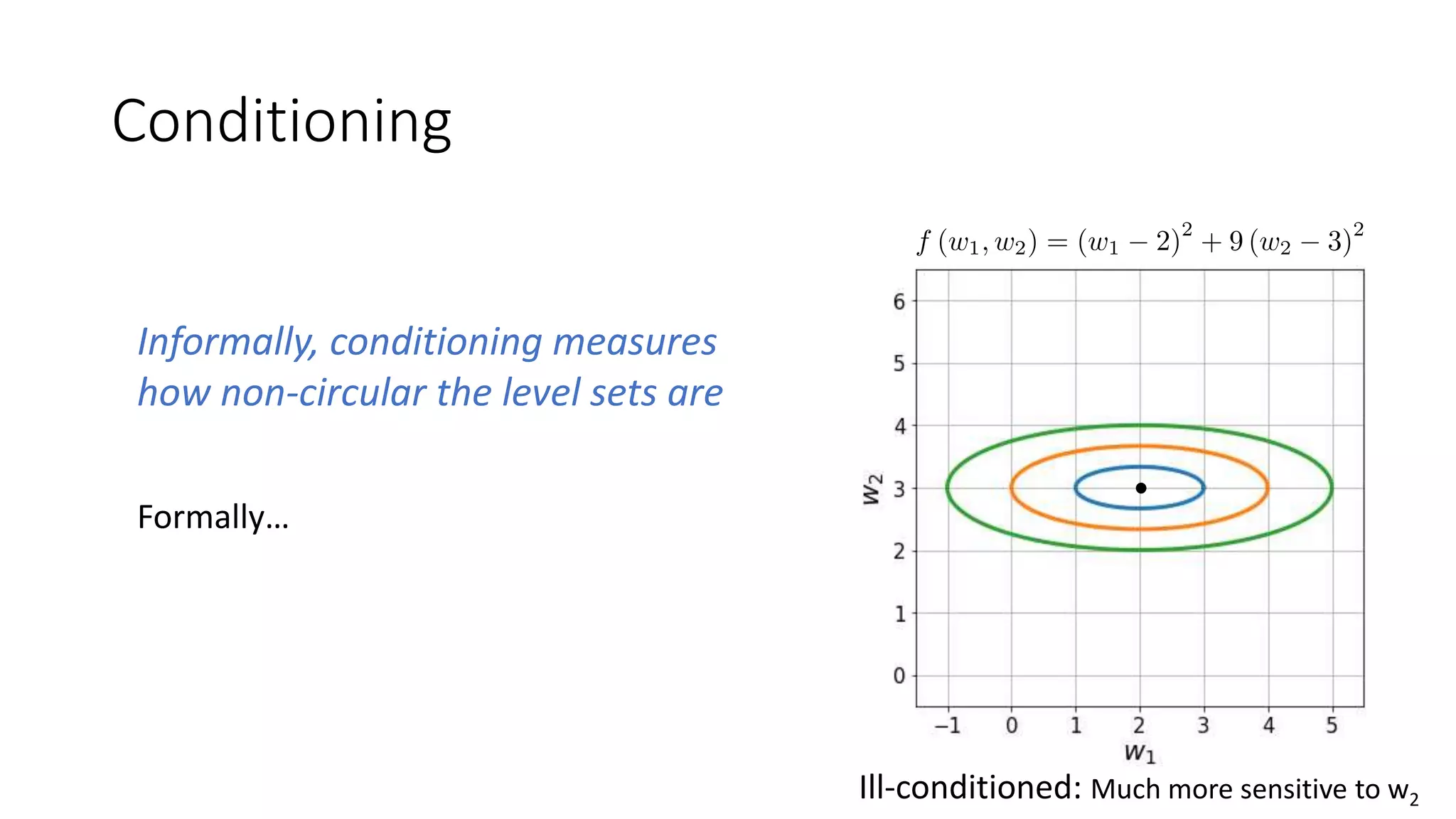
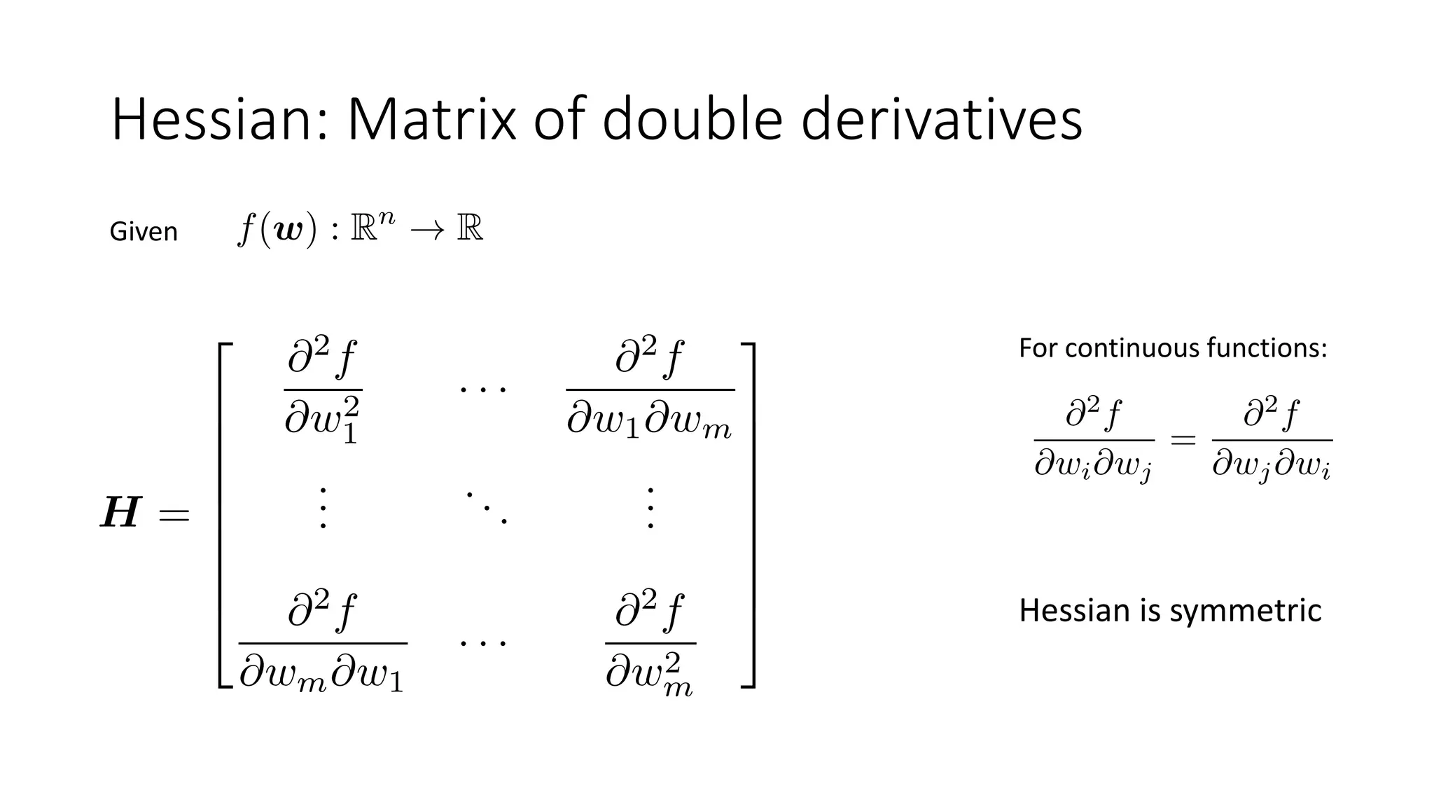
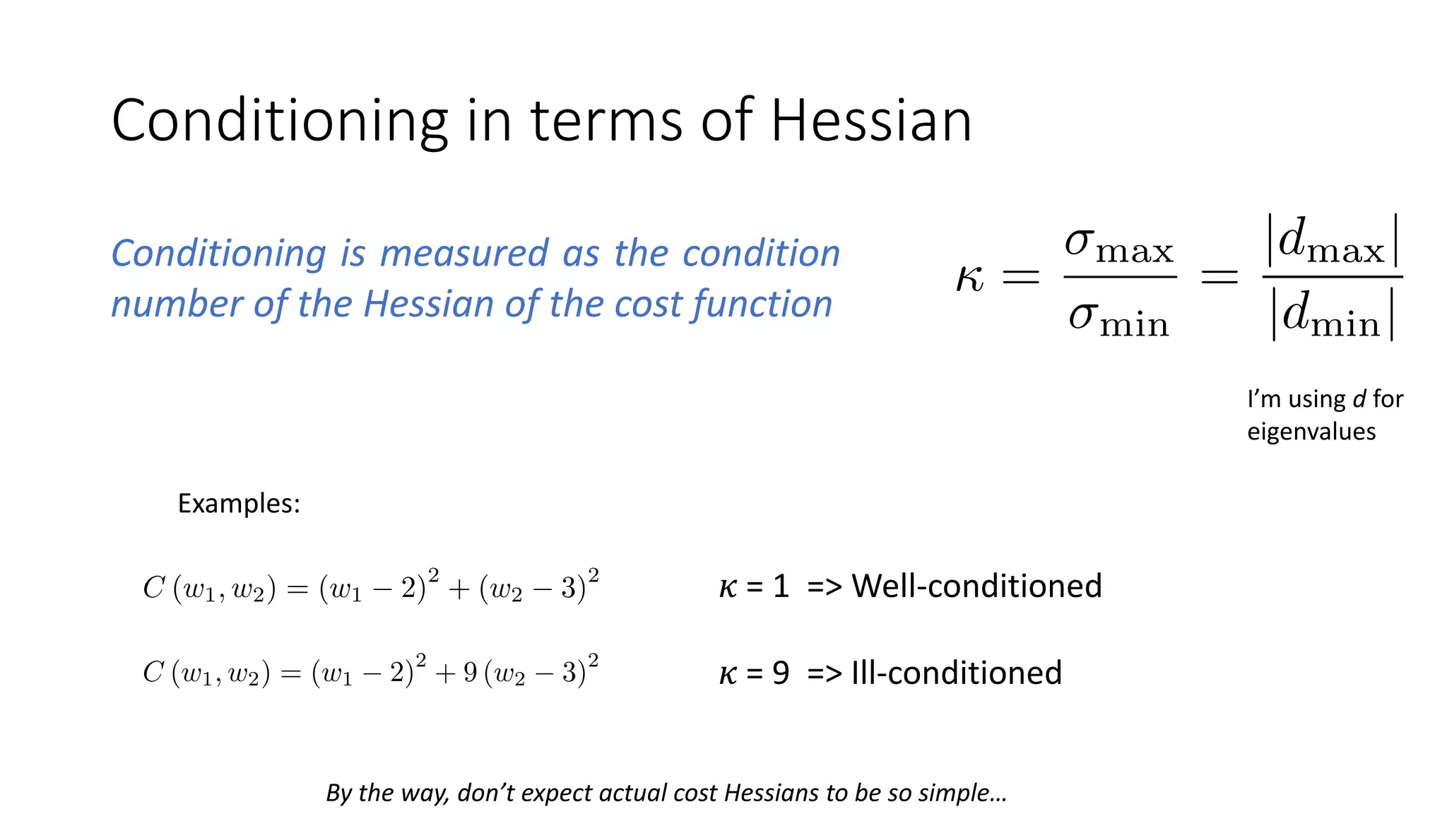
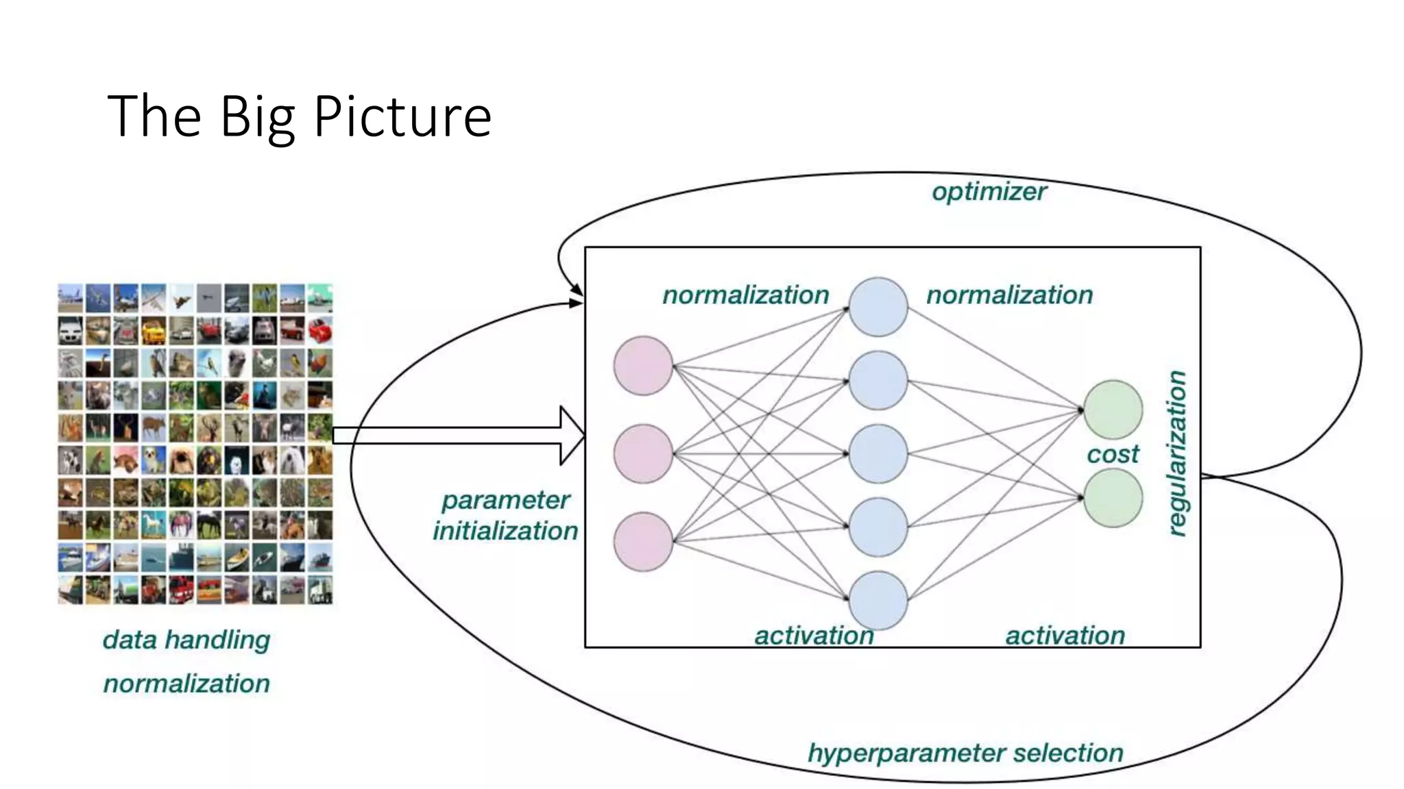
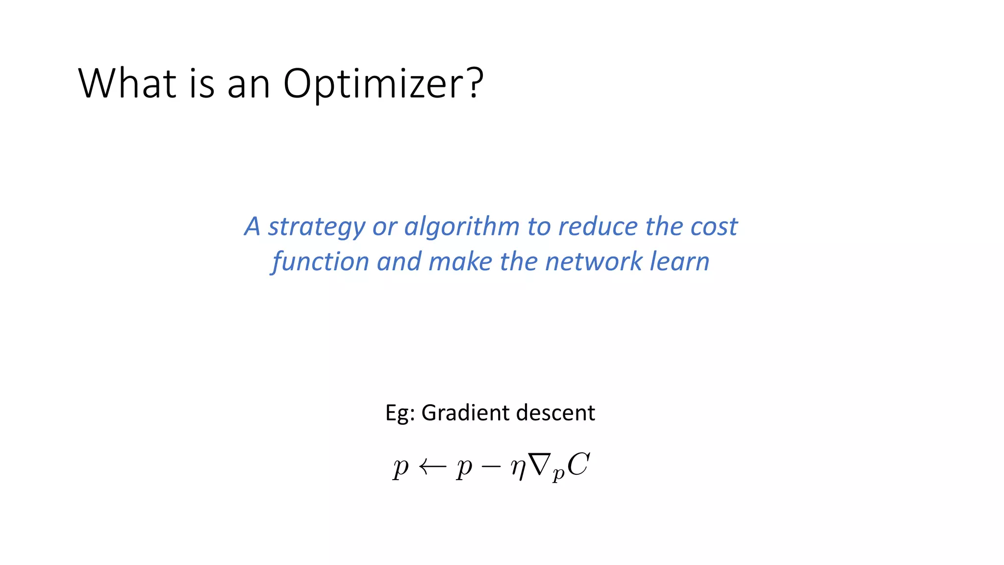
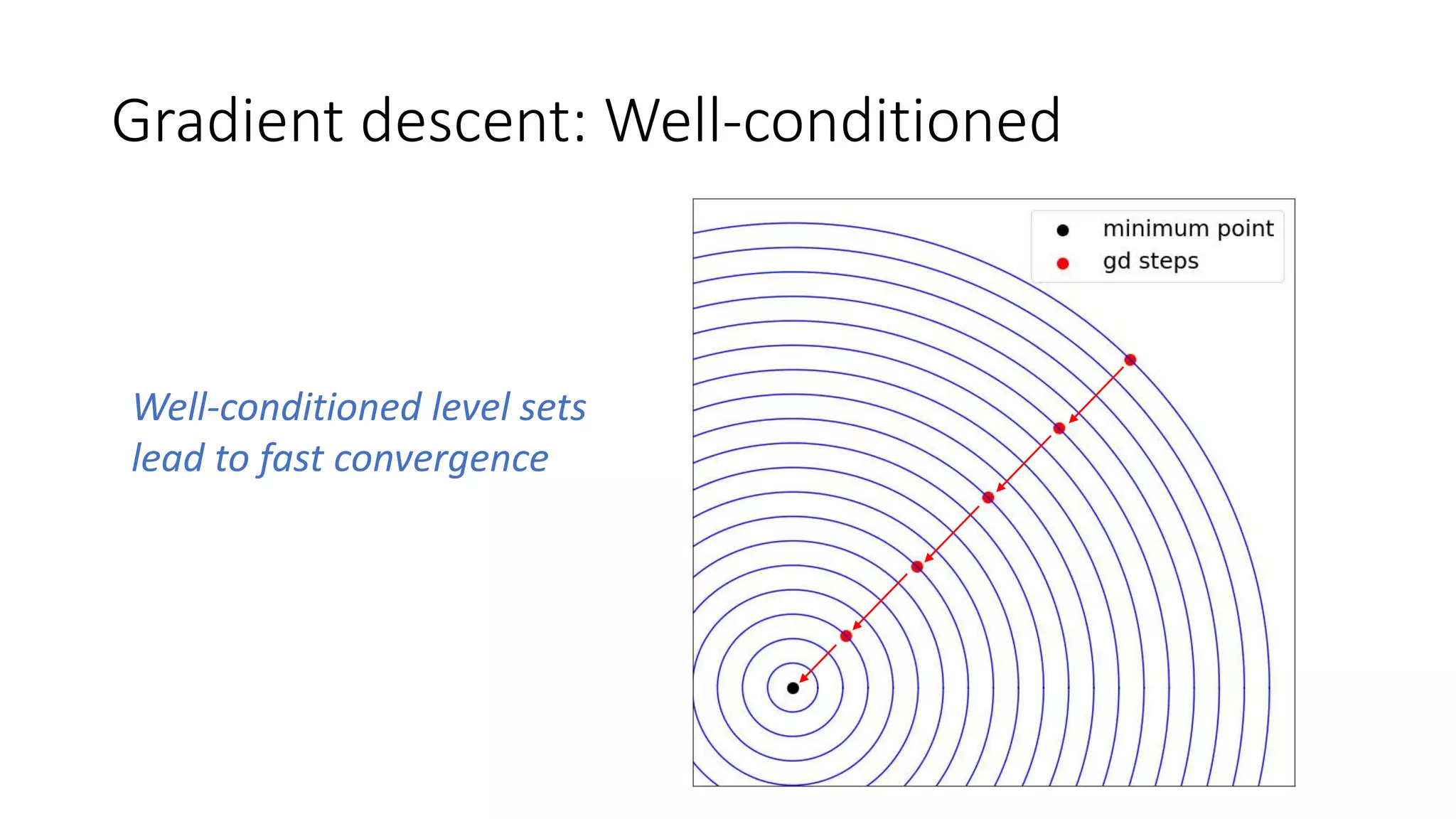
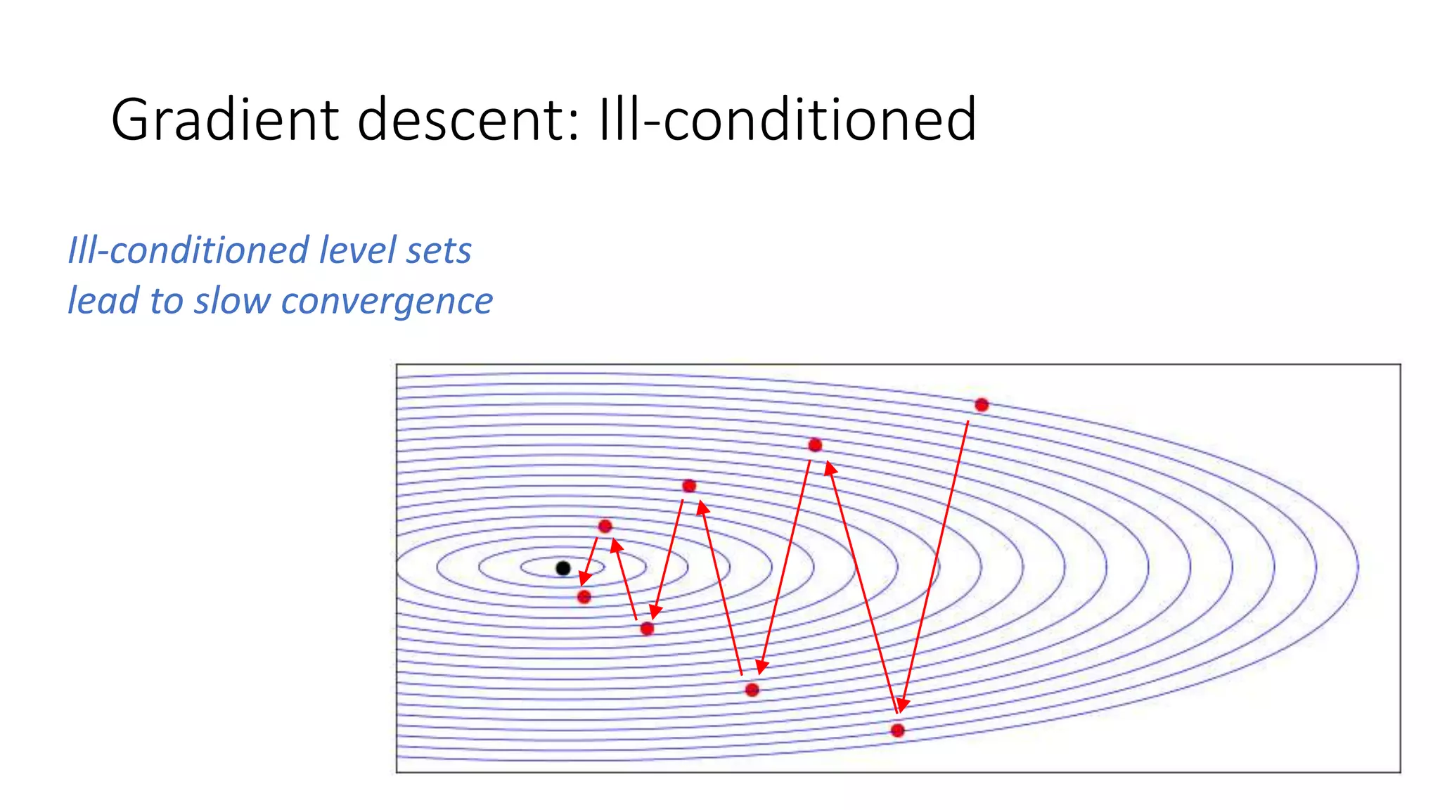
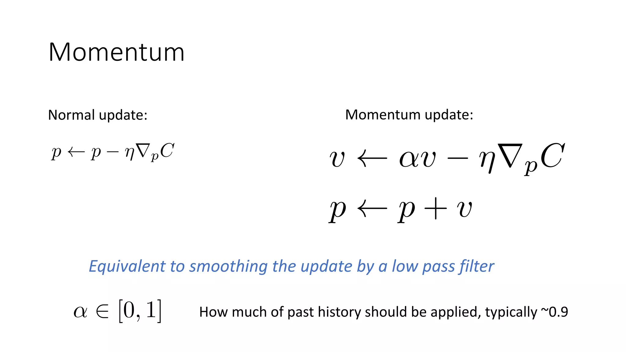
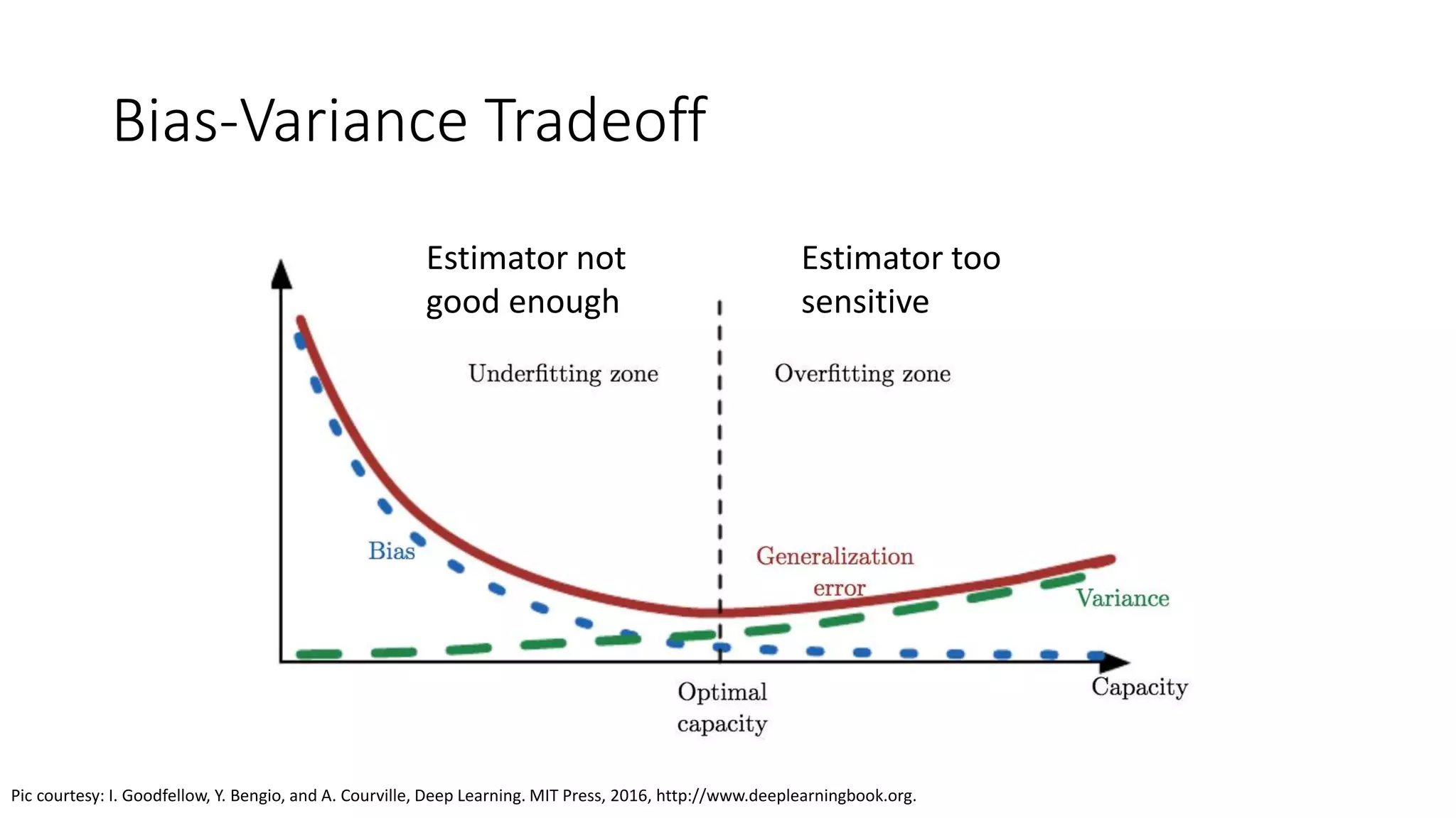
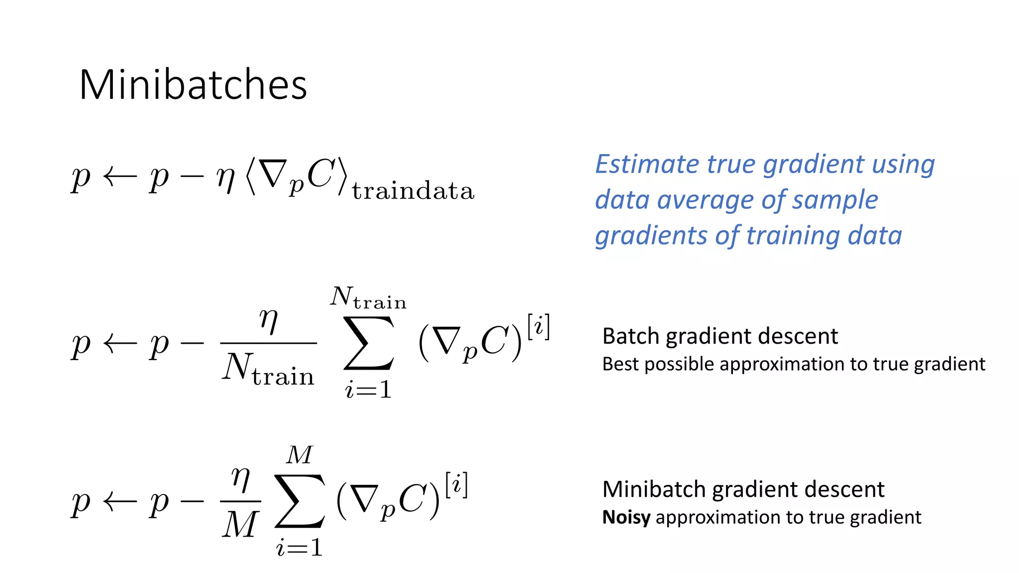
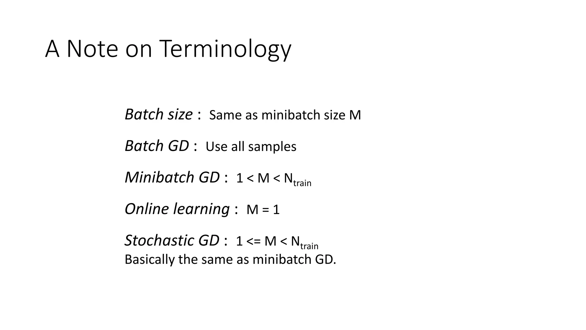
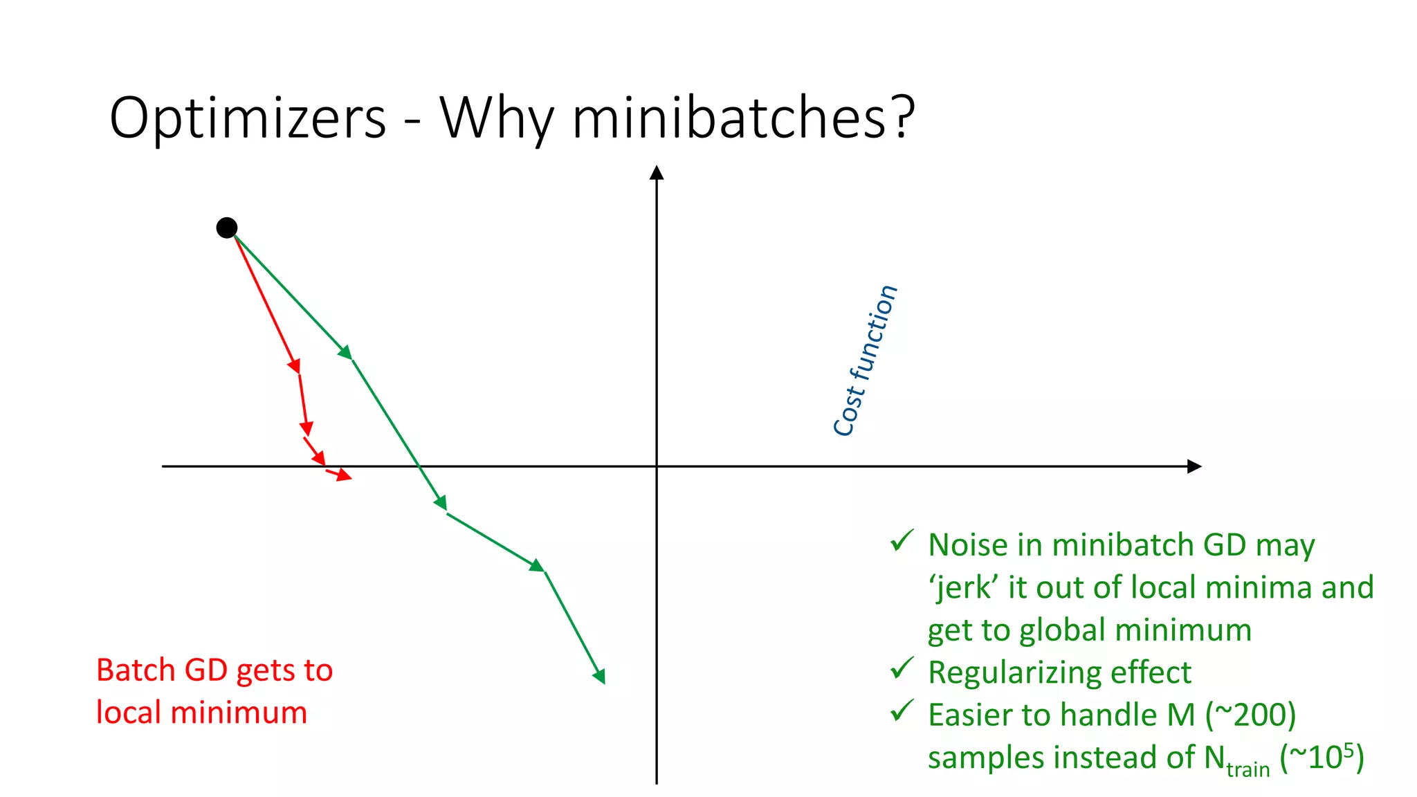
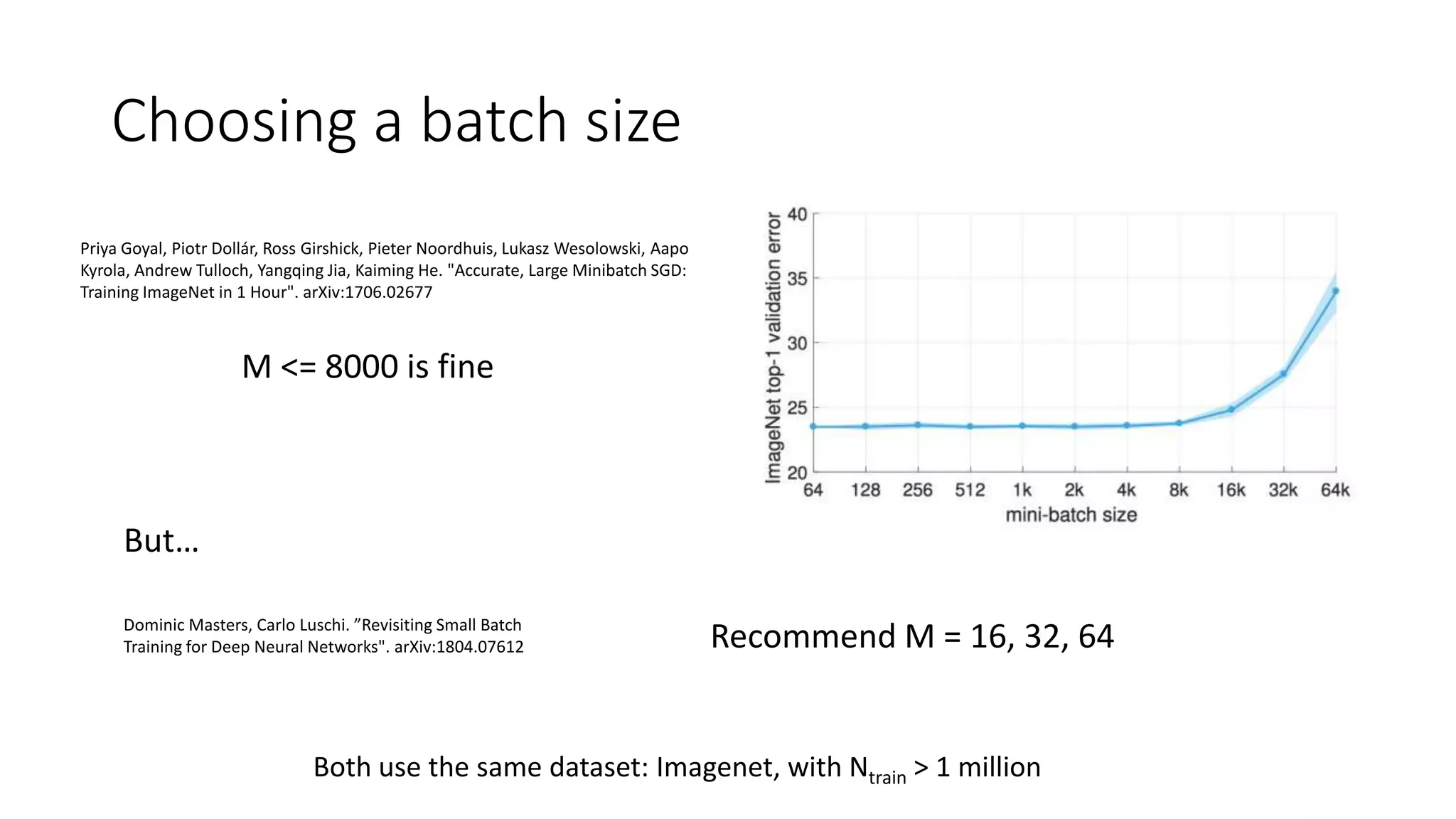
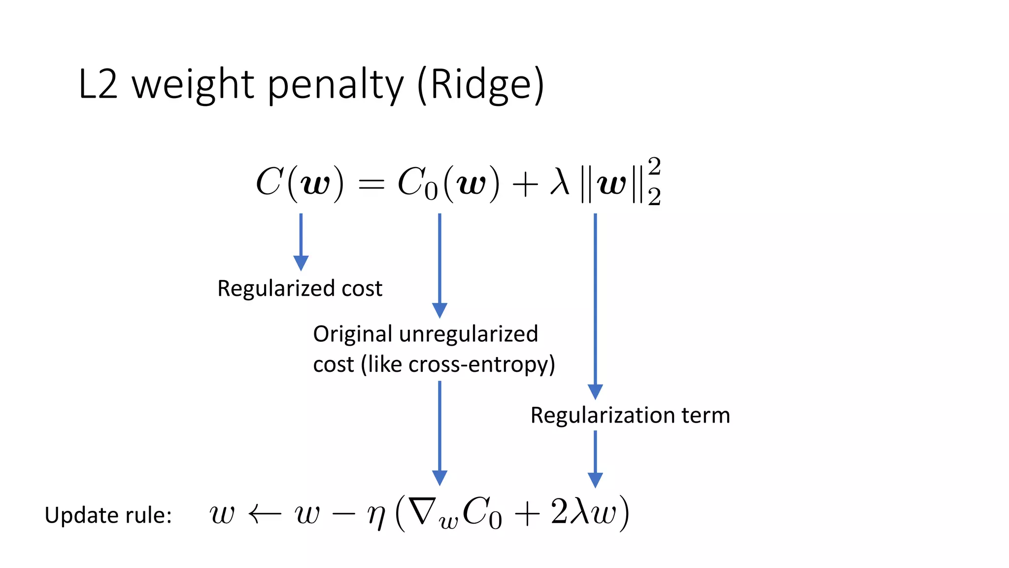
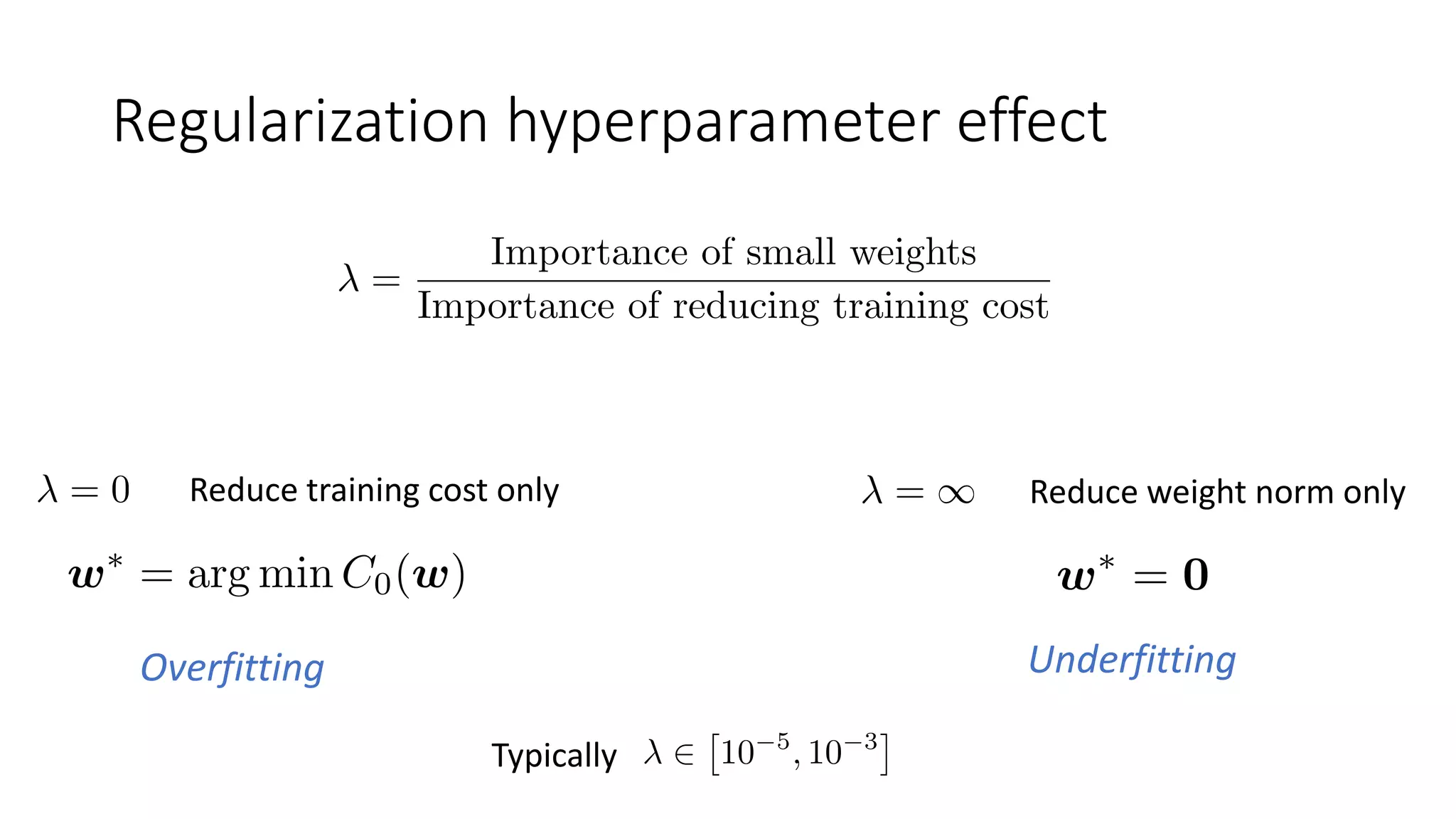
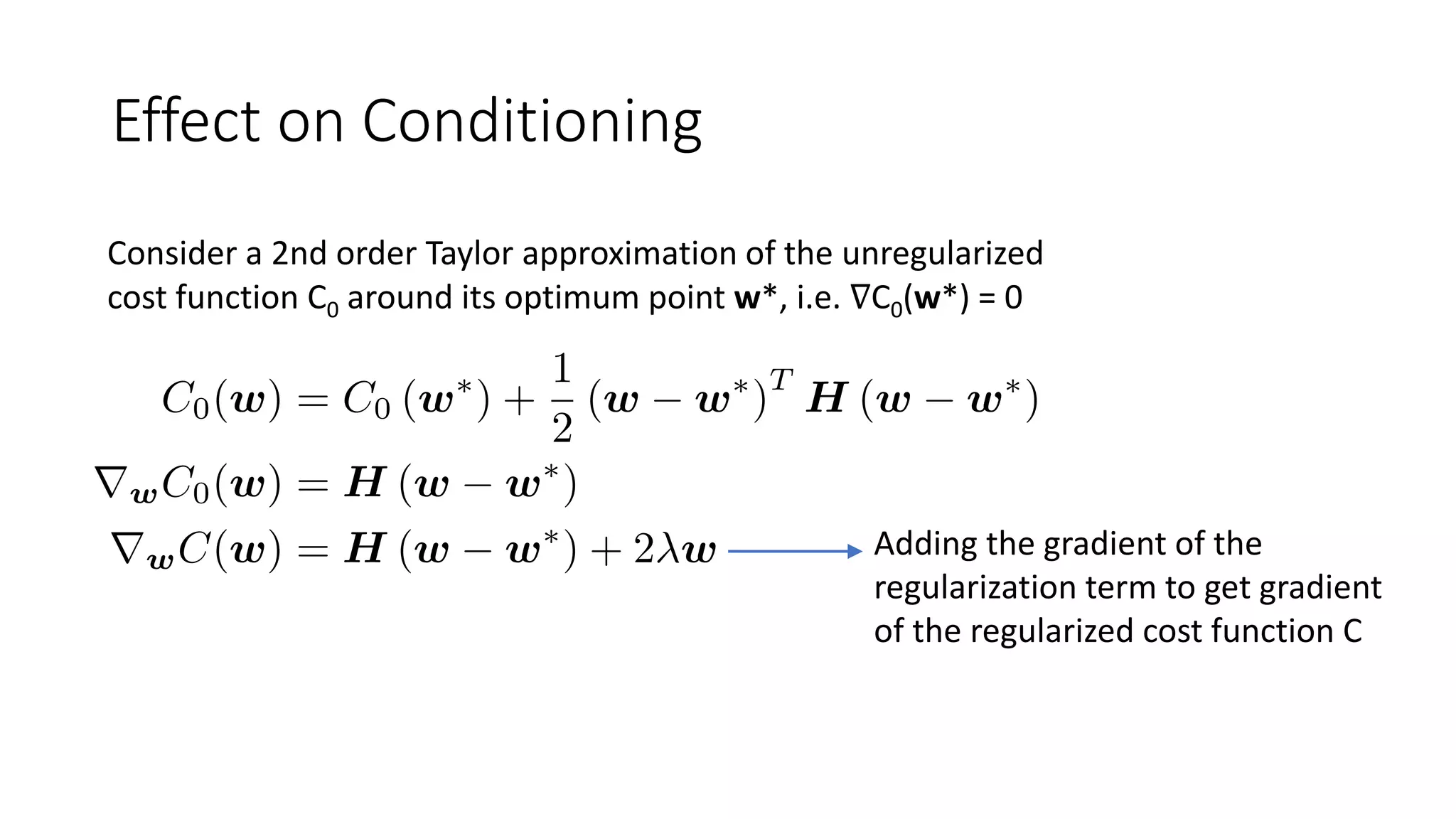
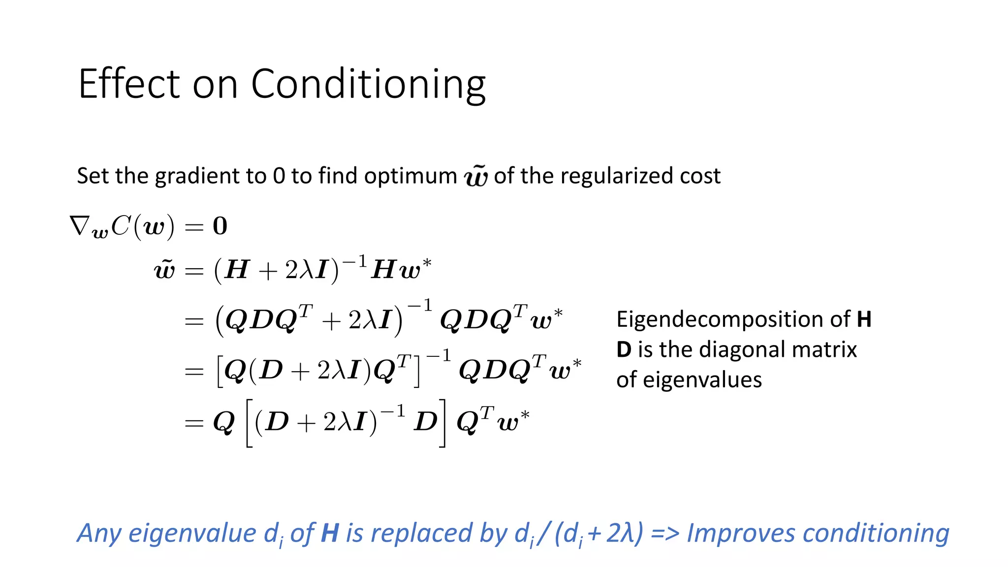
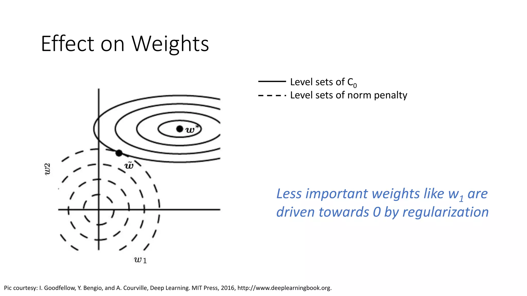
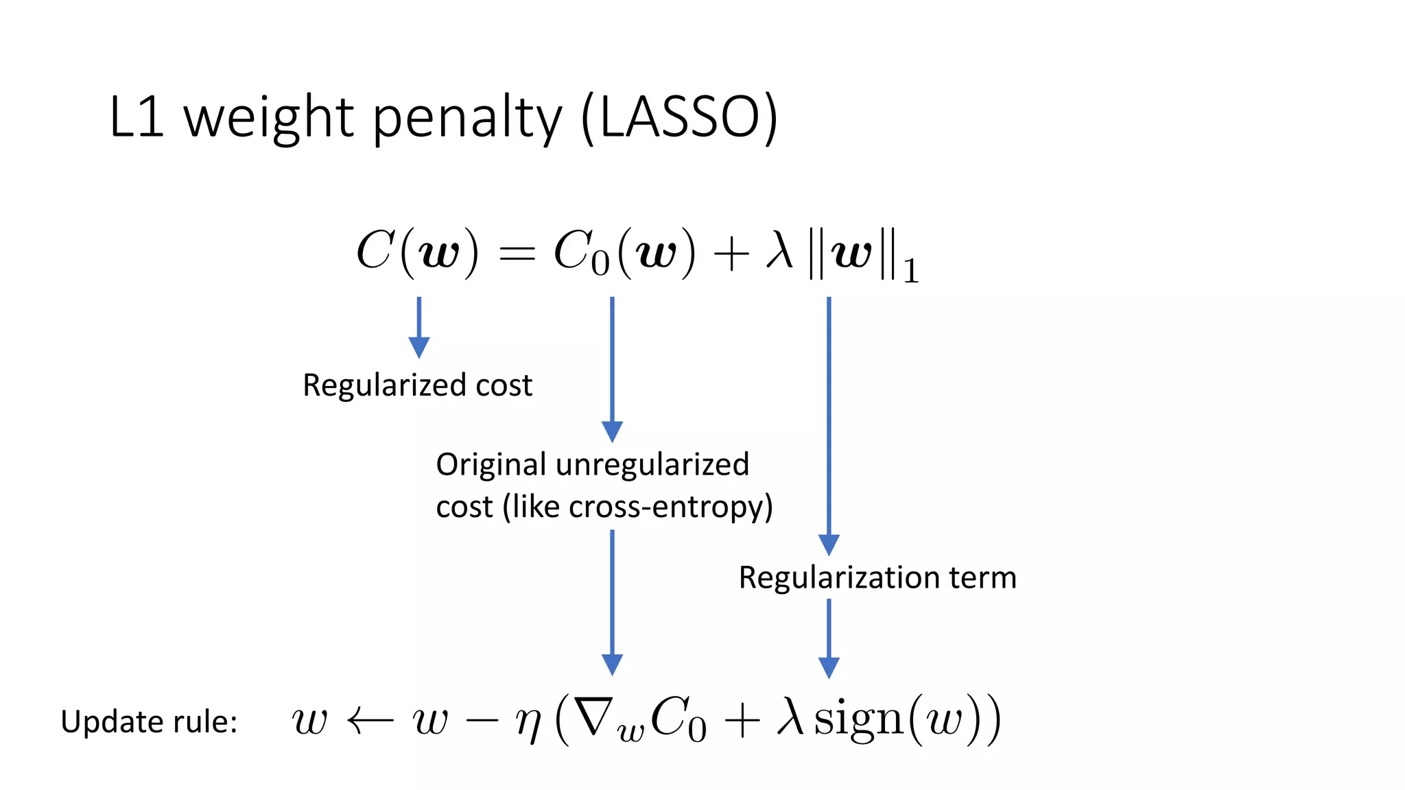
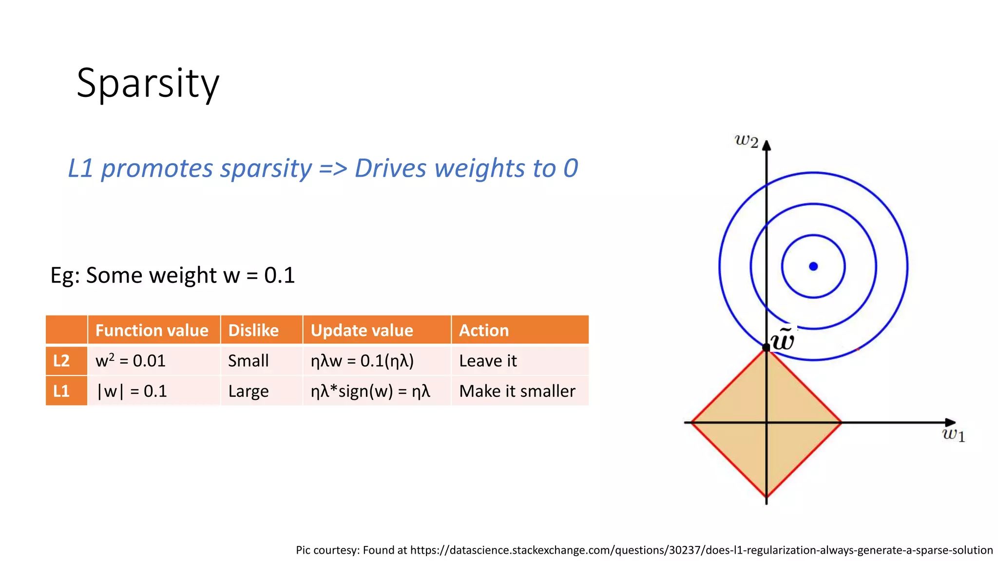
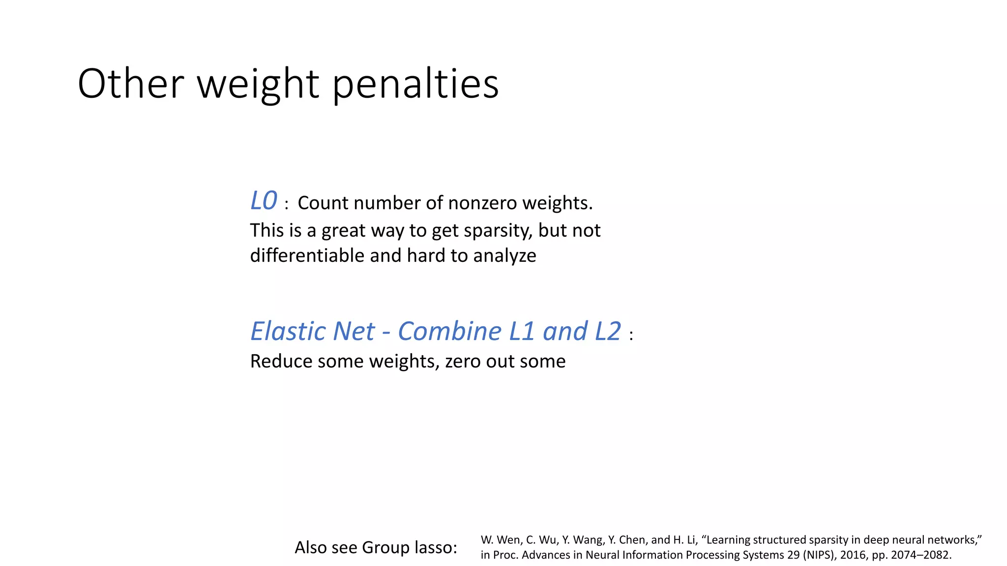
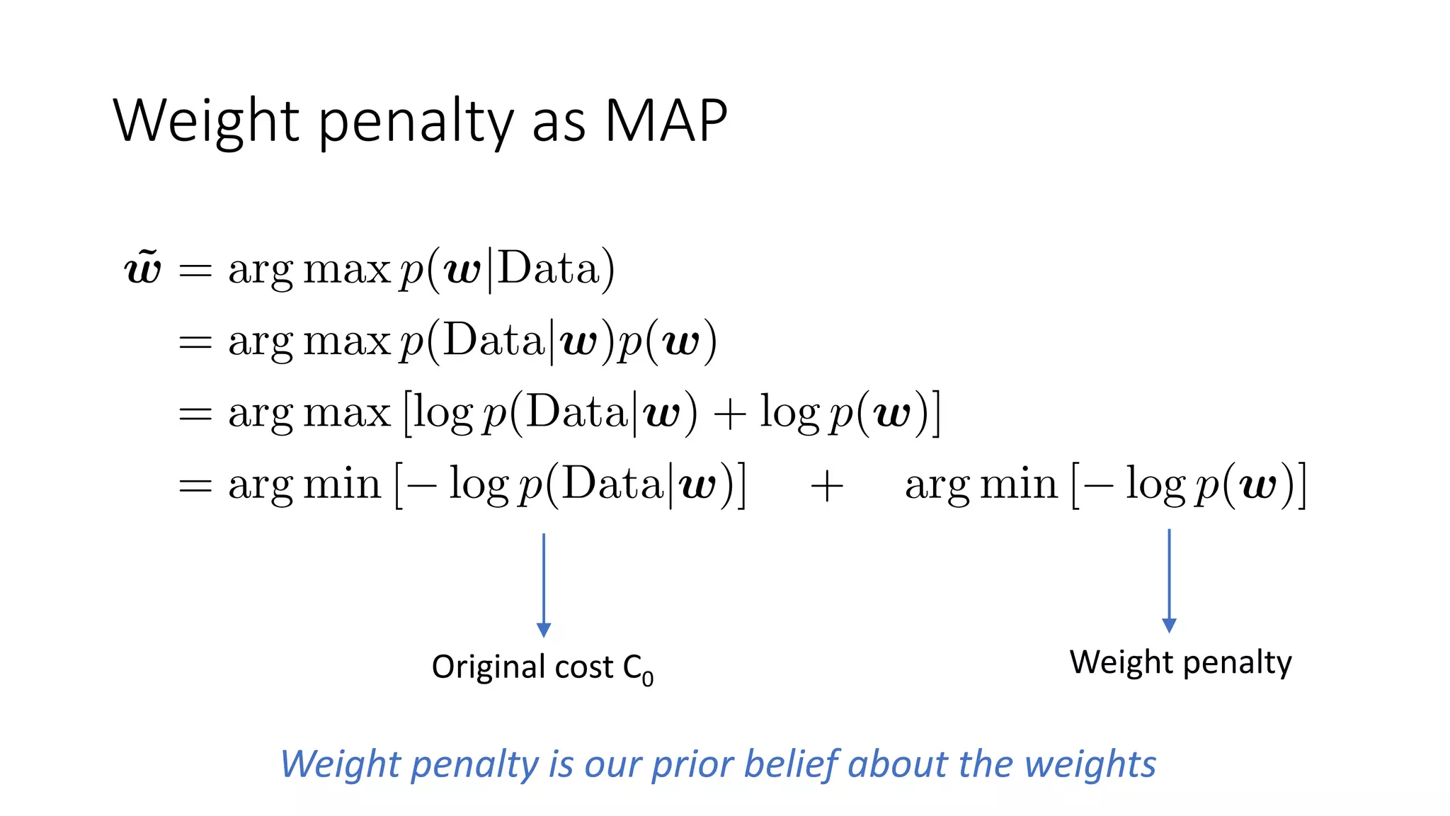
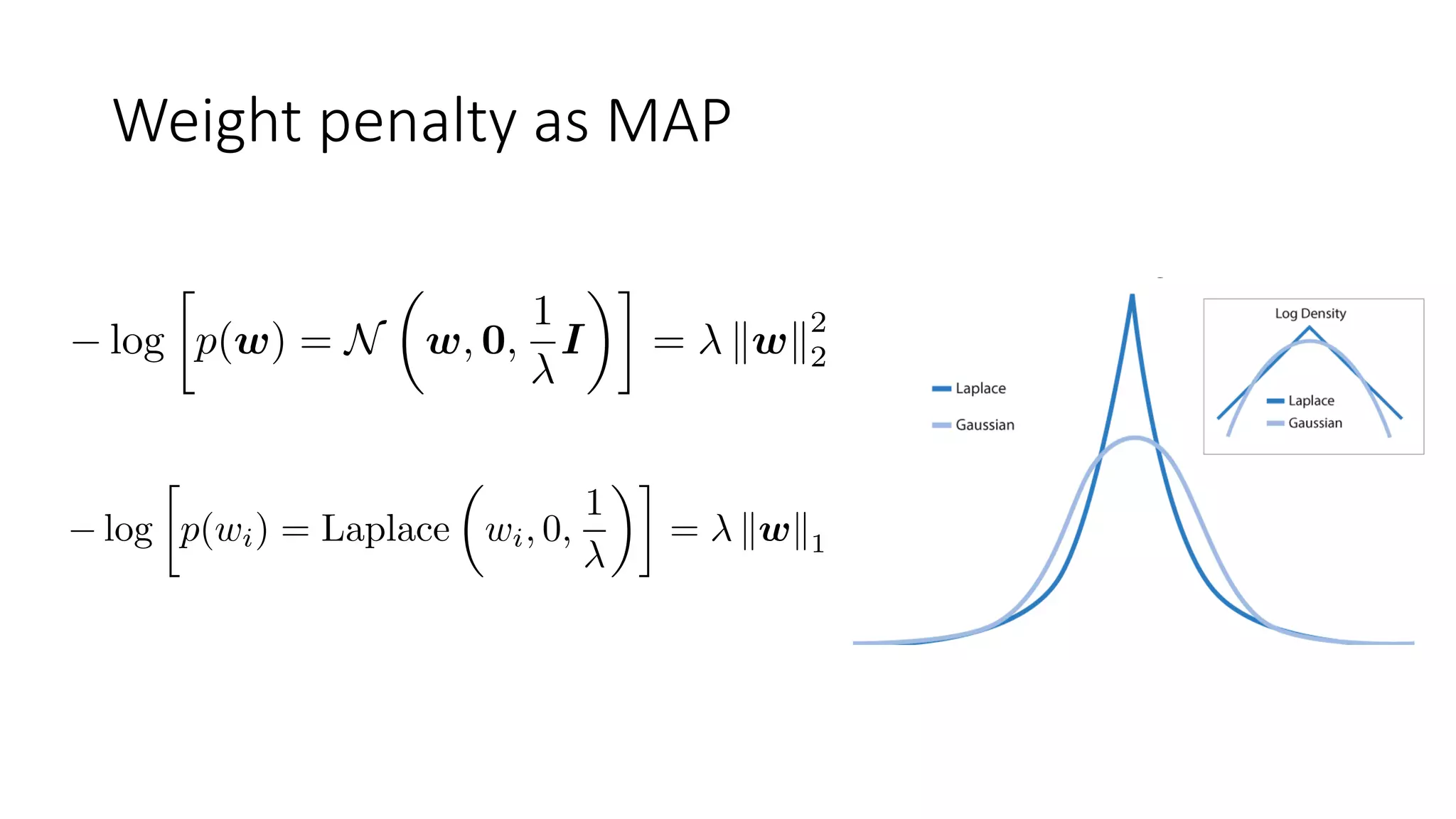
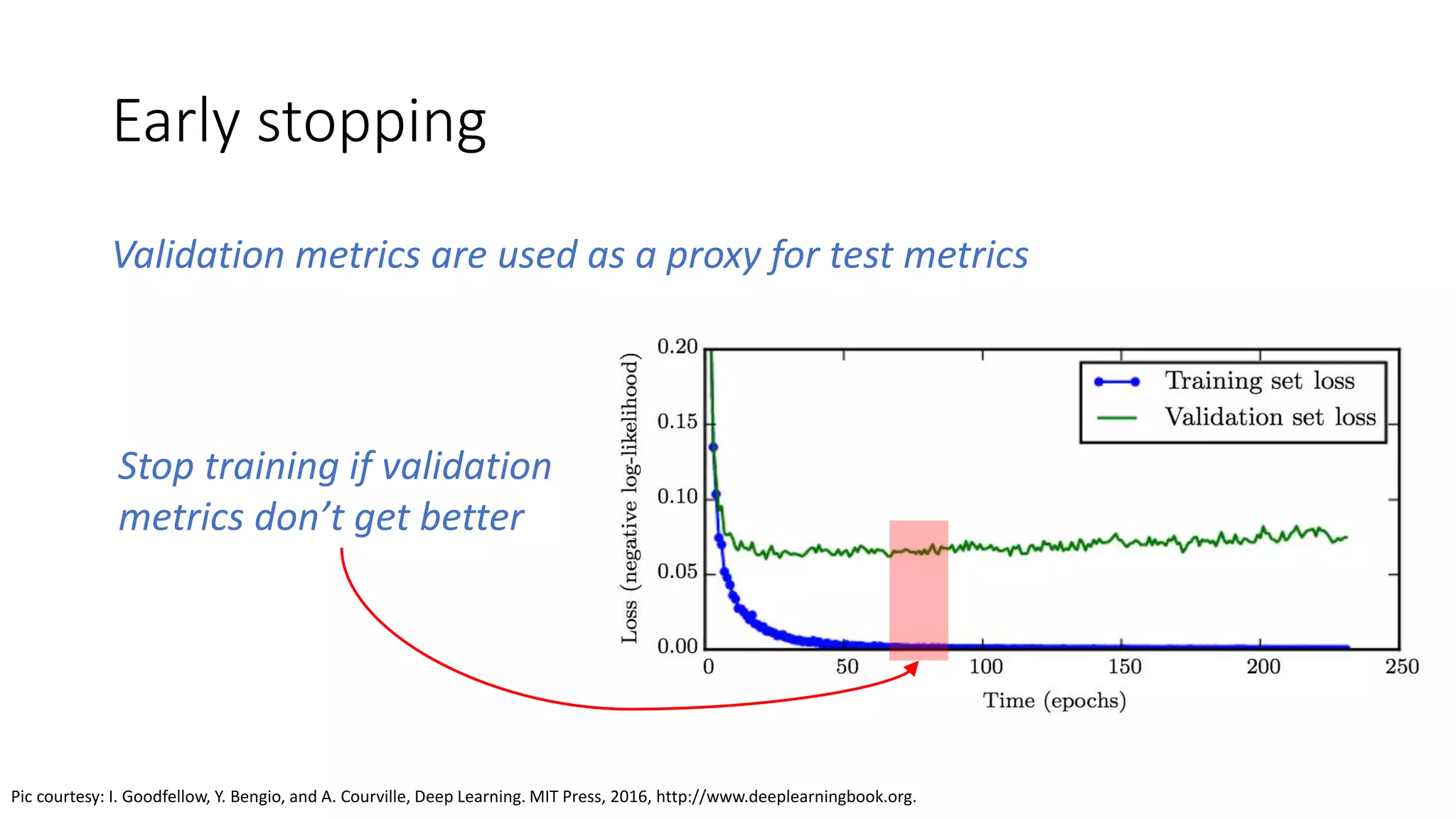
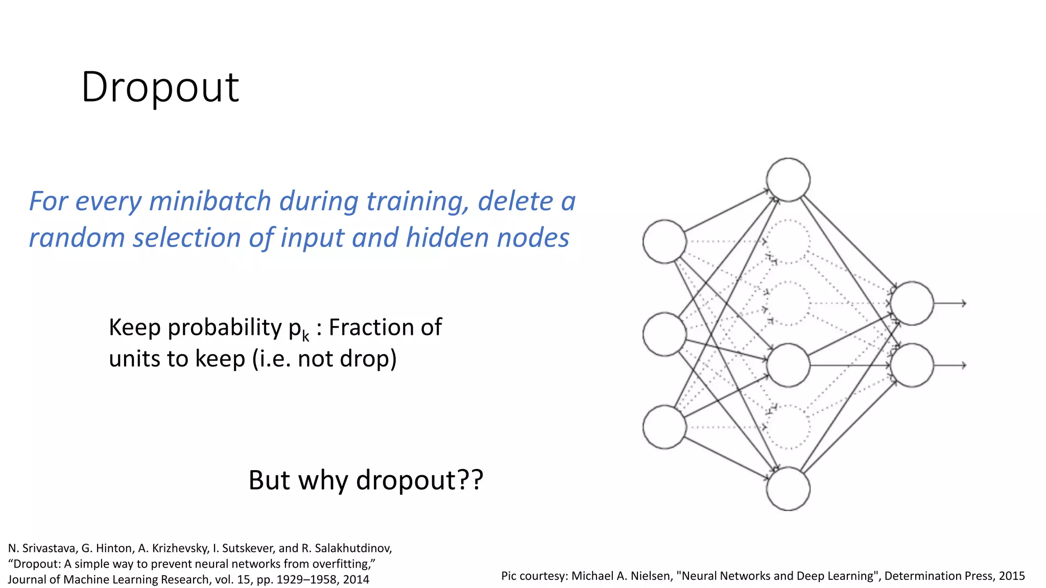
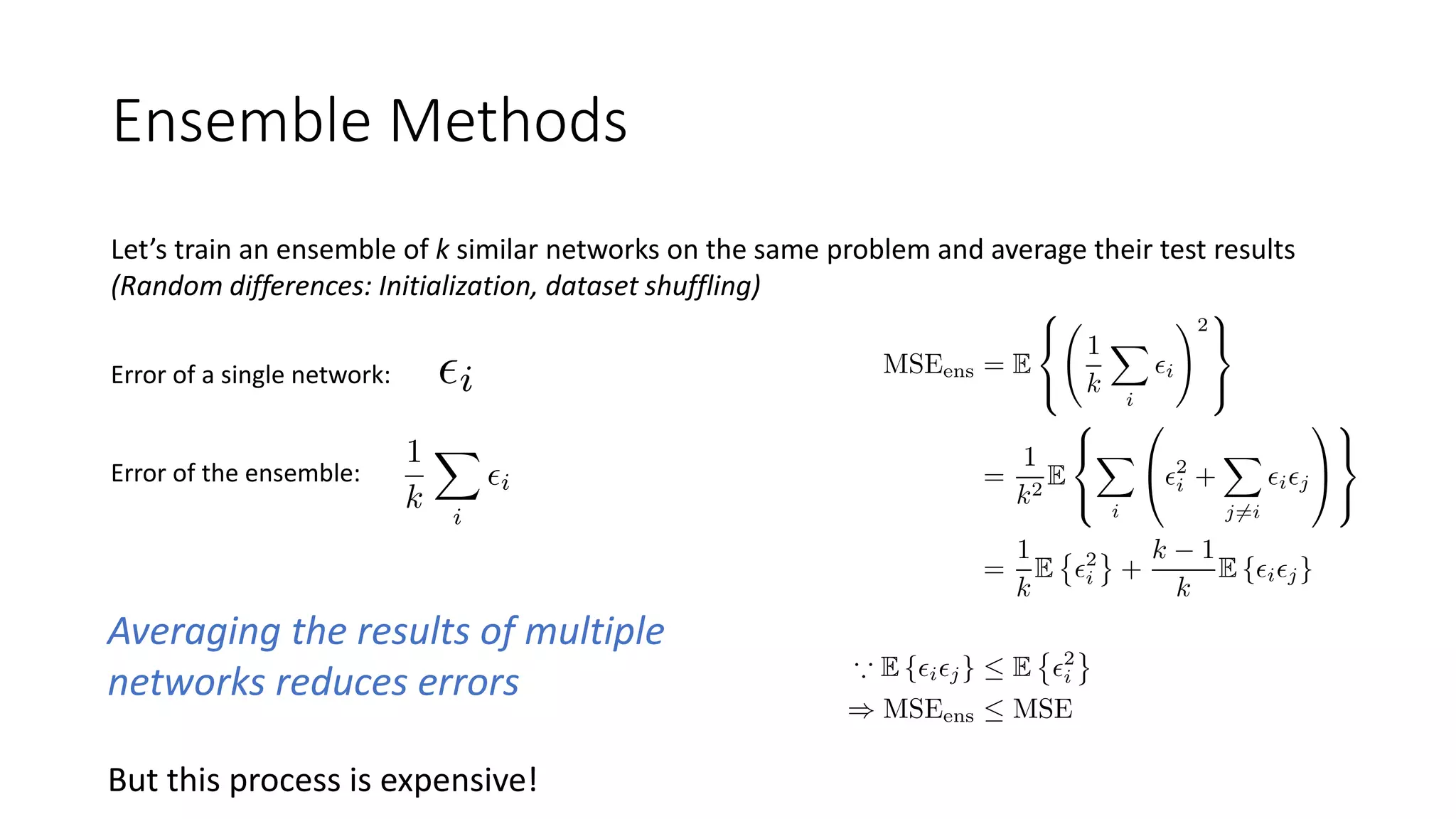
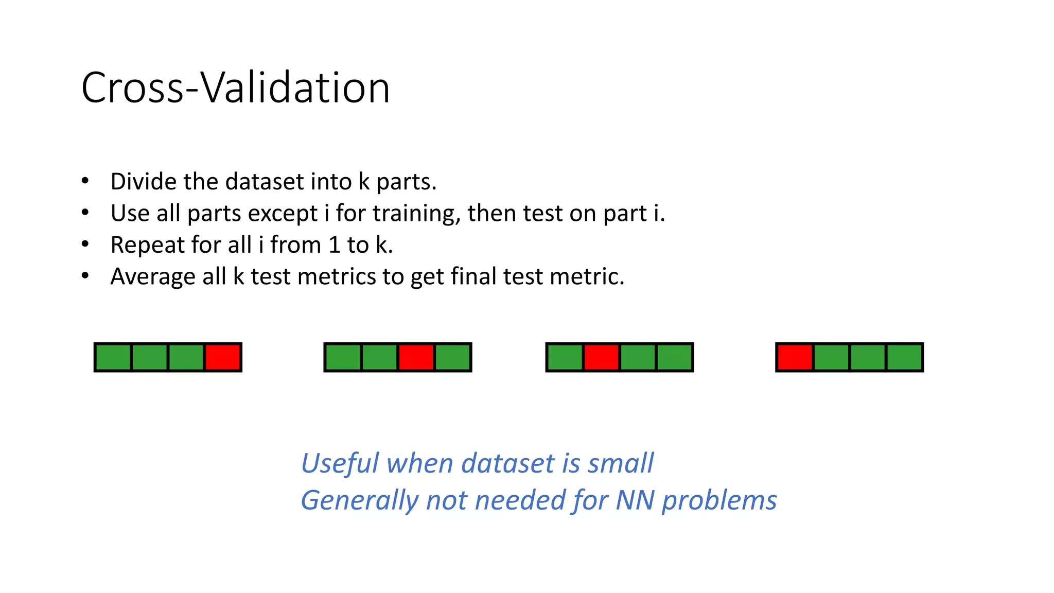
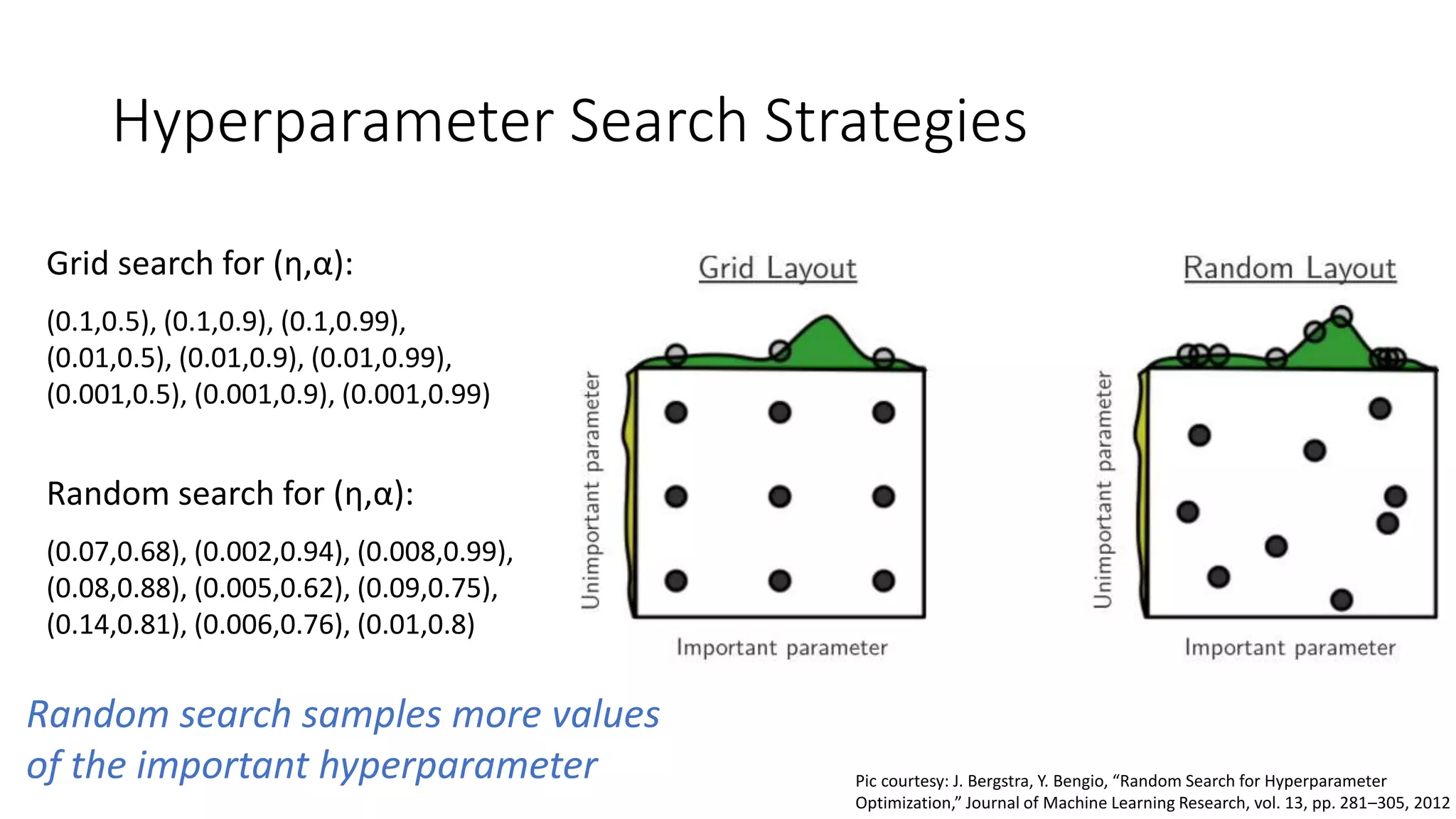
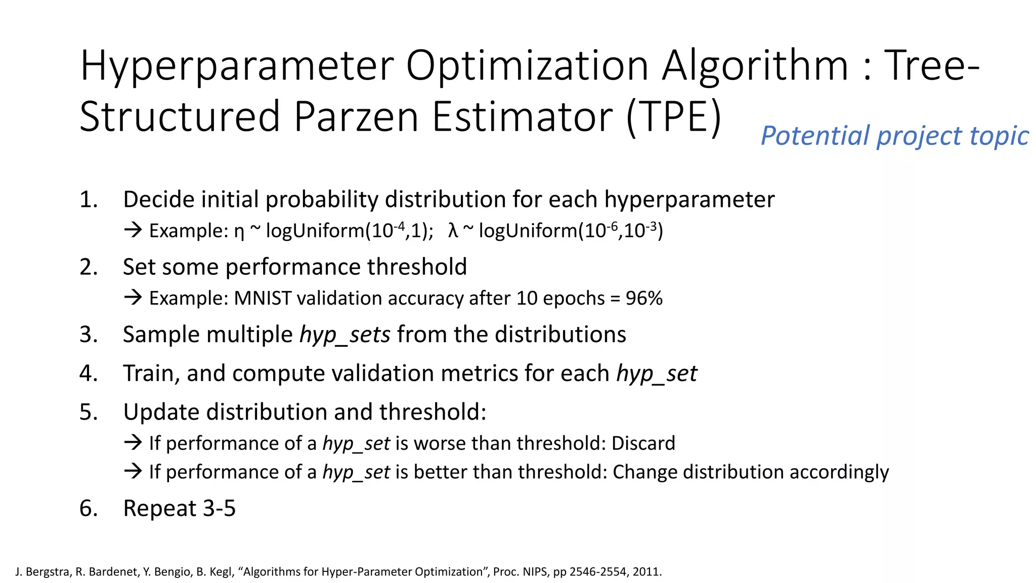
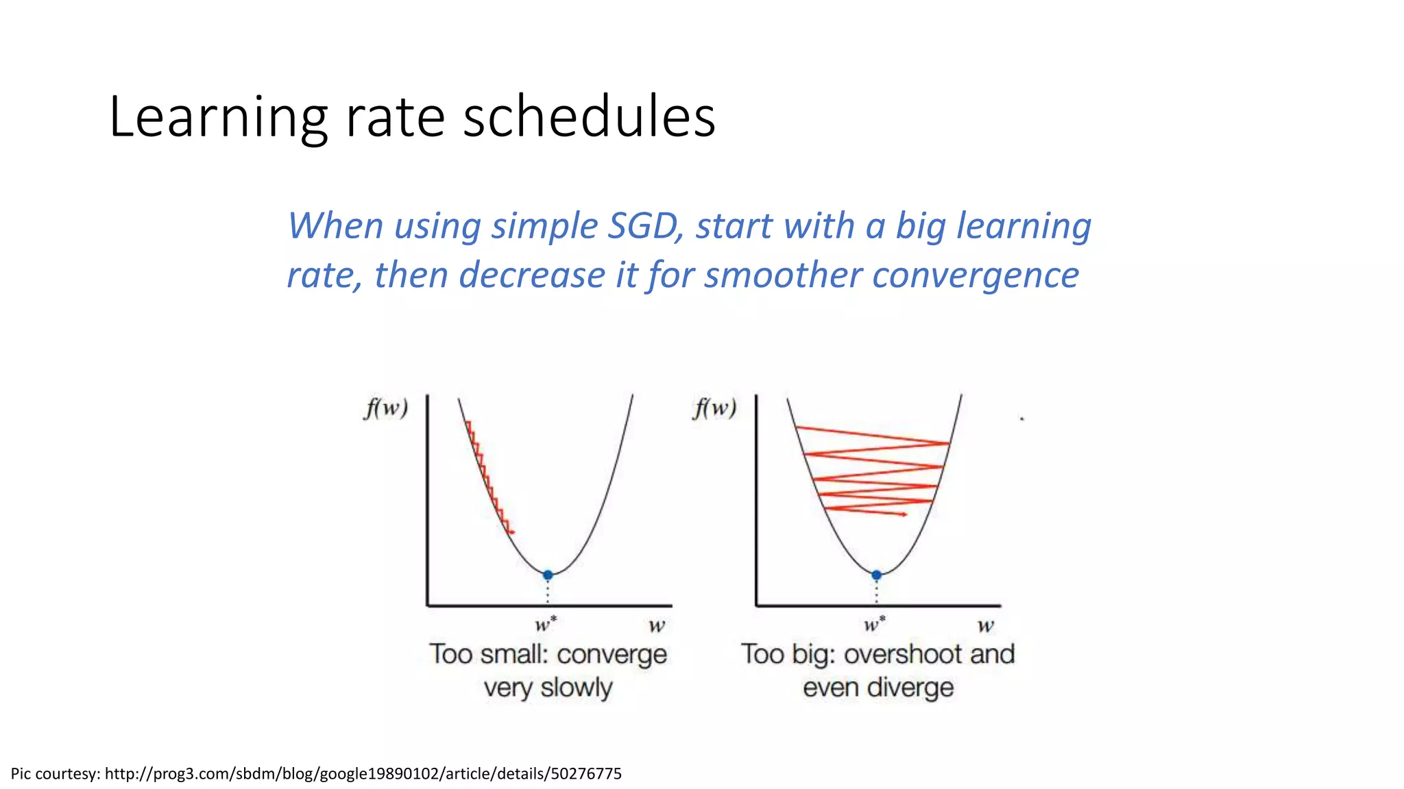
The document discusses various techniques in deep learning, including activation functions, cost functions, optimizers, and regularization. It covers specific methods such as ReLU, dropout, and different types of weight penalties like L1 and L2, along with their impacts on model performance. Additionally, the document emphasizes the importance of hyperparameter selection, parameter initialization, and strategies for addressing overfitting in neural networks.