This document provides an overview of deep learning including:
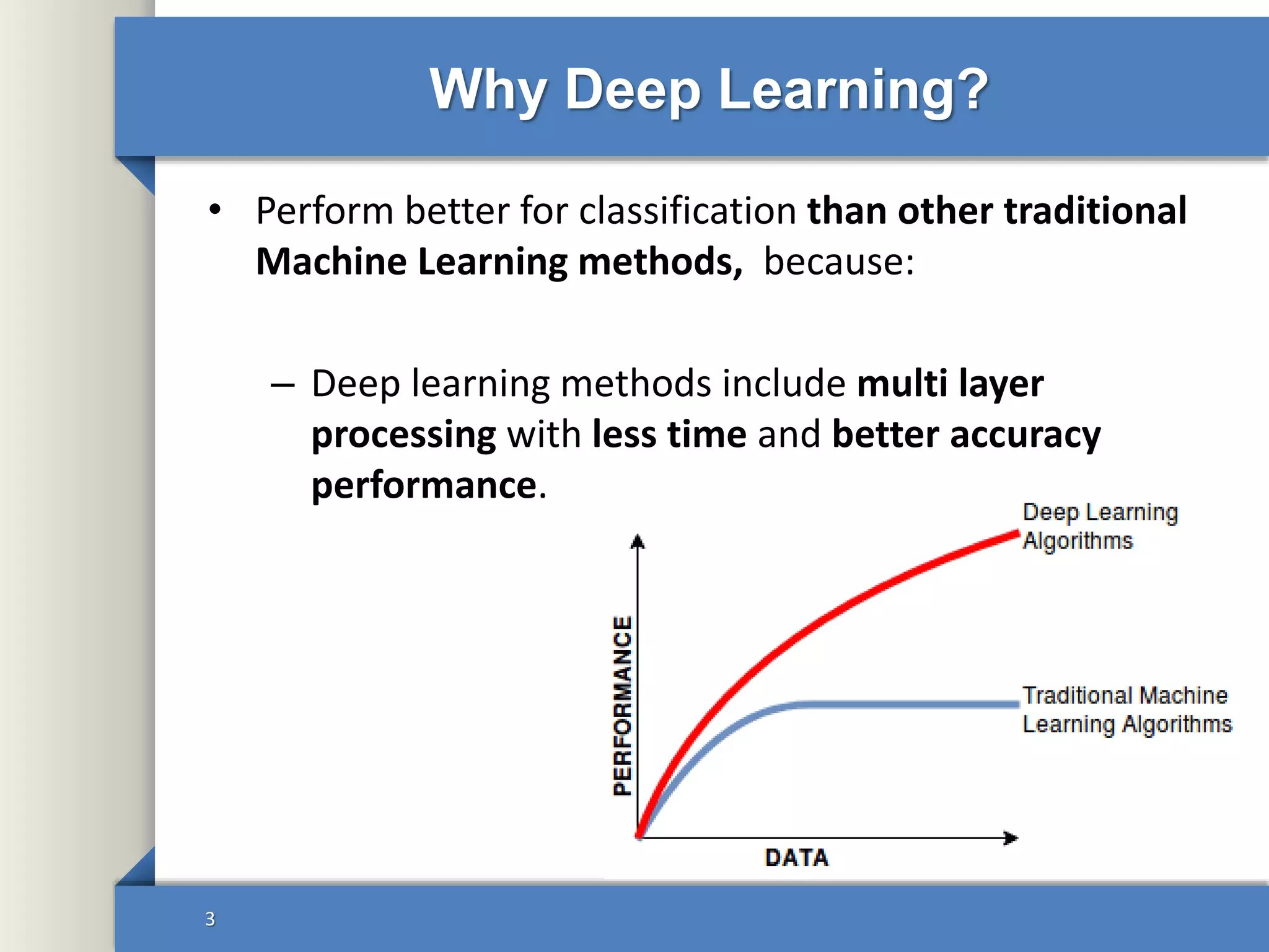
1. Why deep learning performs better than traditional machine learning for tasks like image and speech recognition.
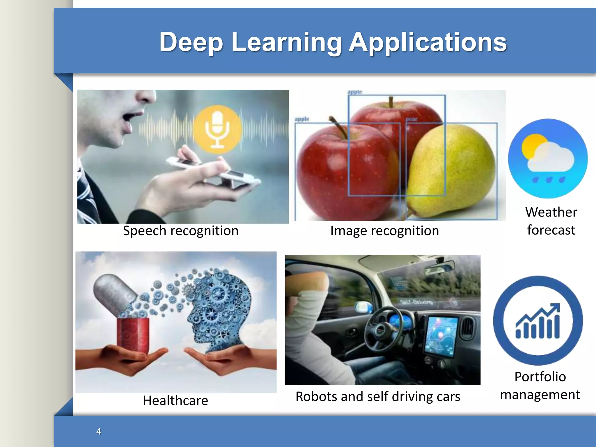
2. Common deep learning applications such as image recognition, speech recognition, and healthcare.
3. Challenges of deep learning like the need for large datasets and lack of interpretability.