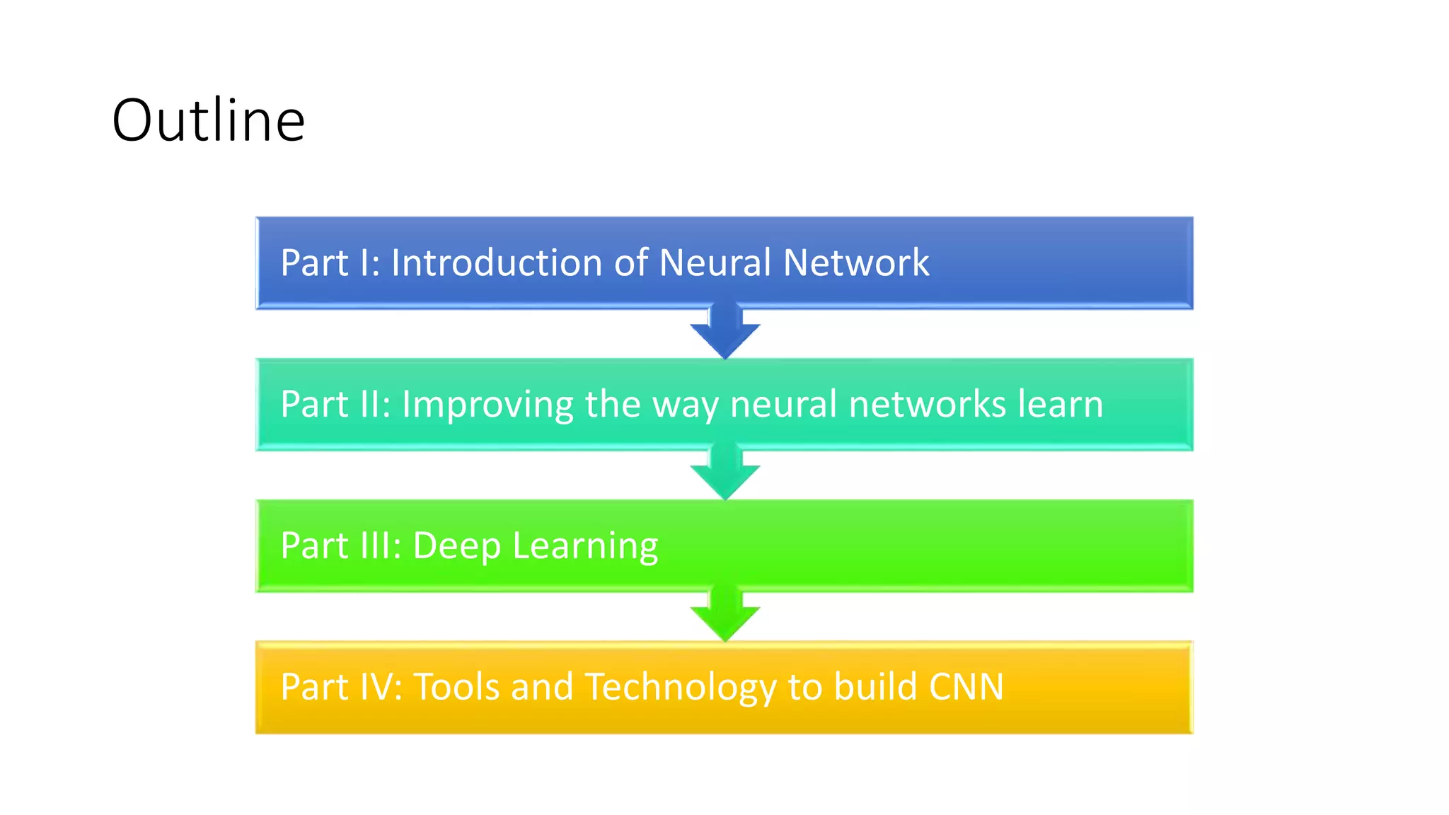
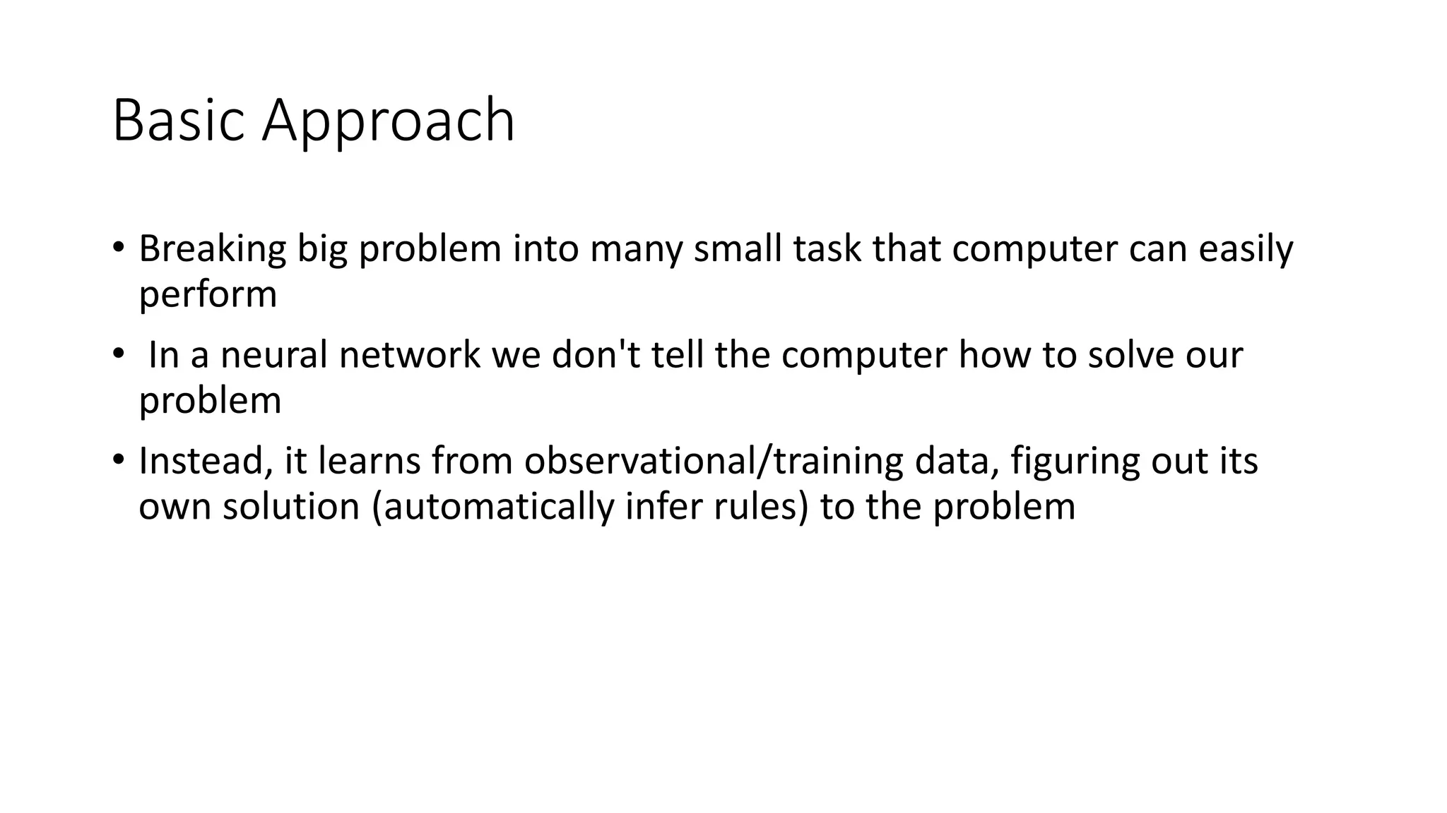
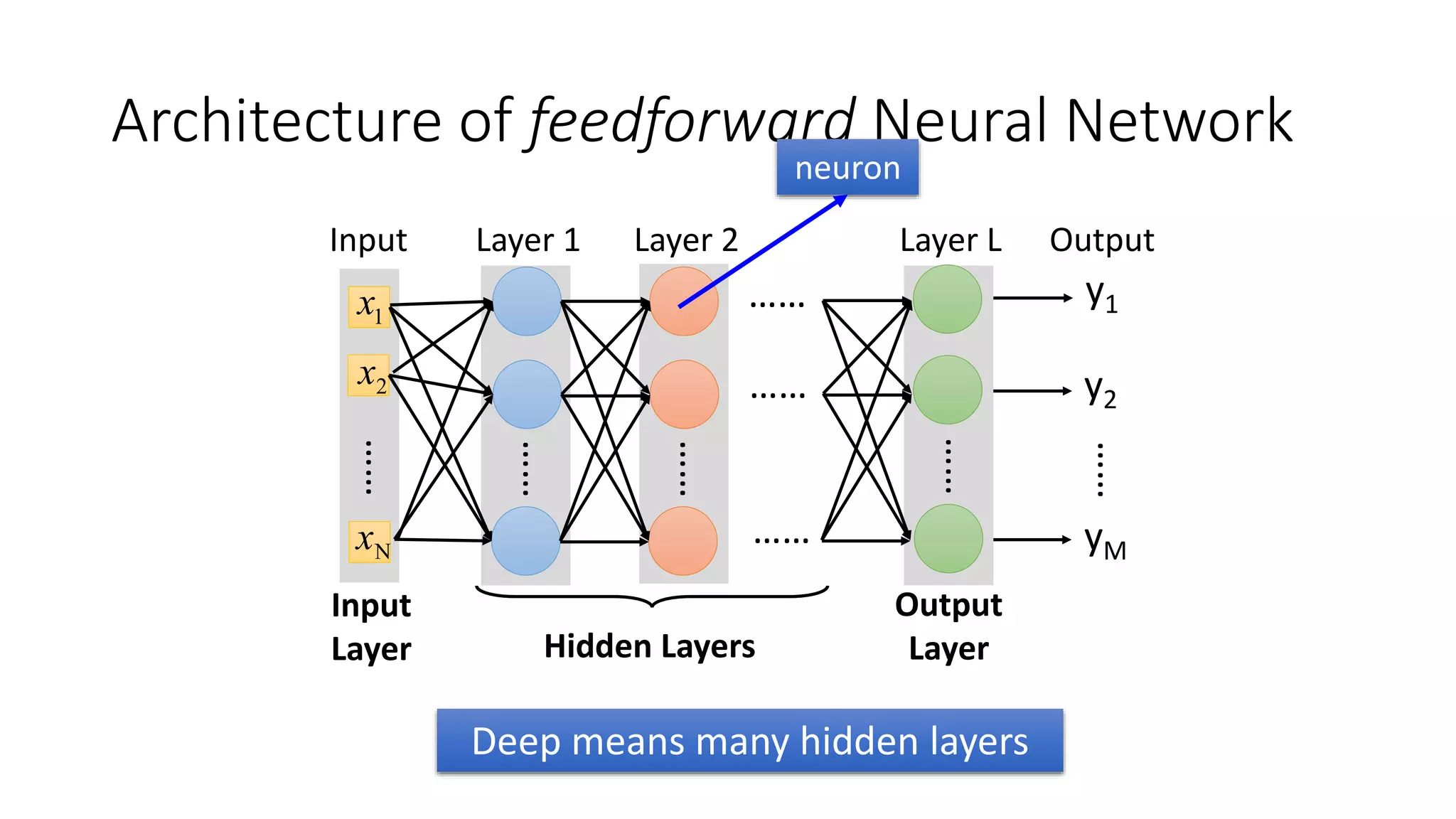
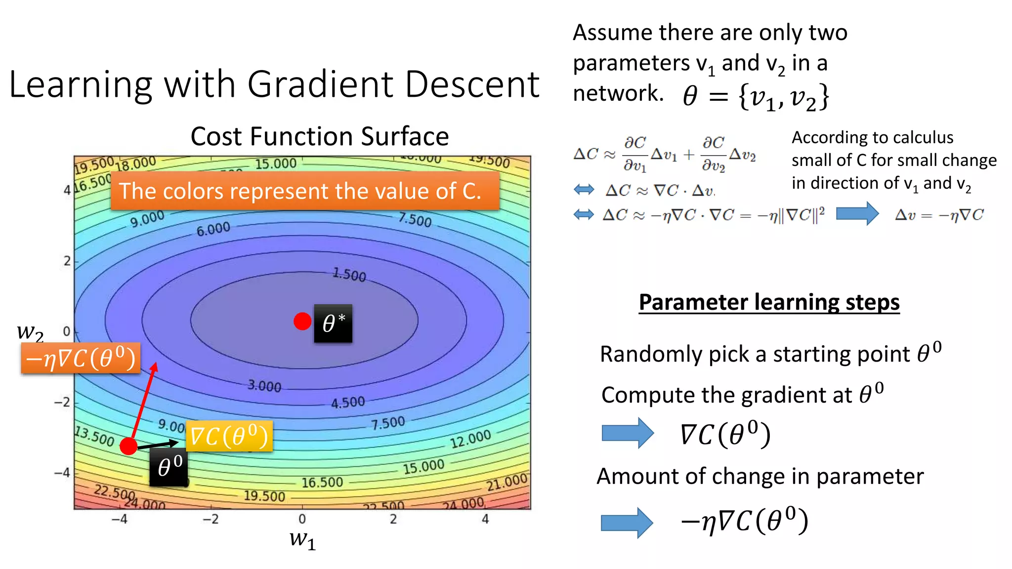
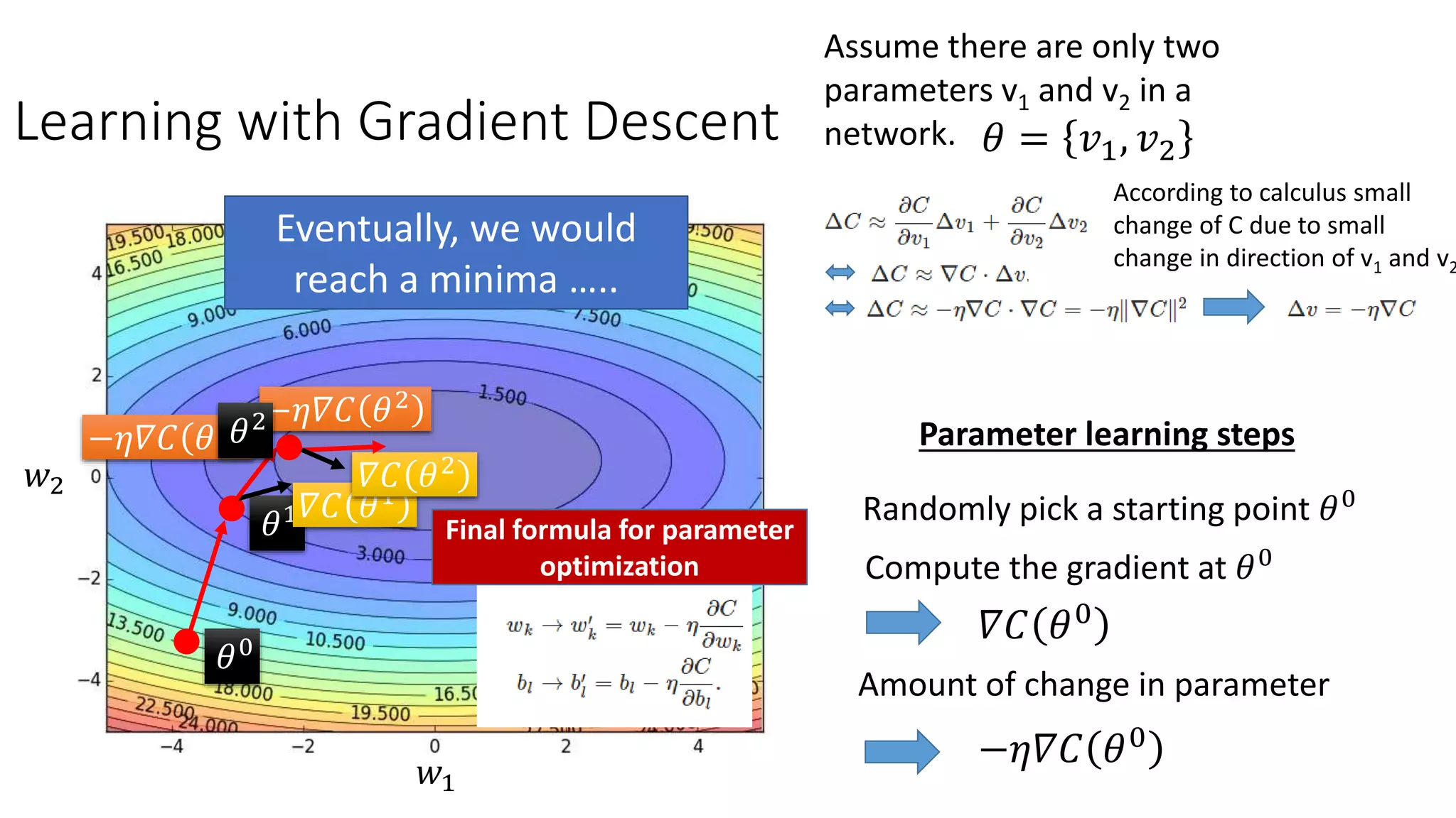
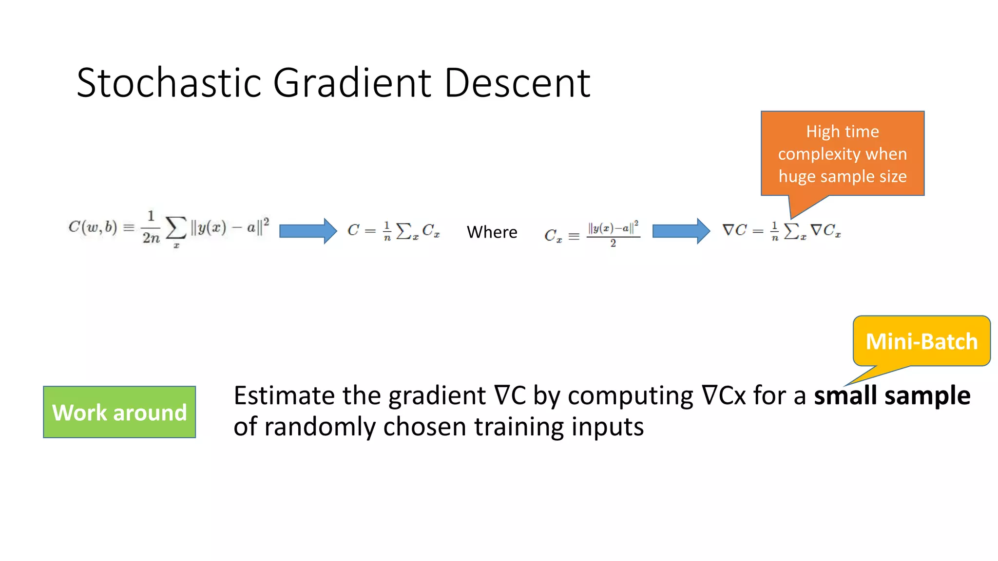
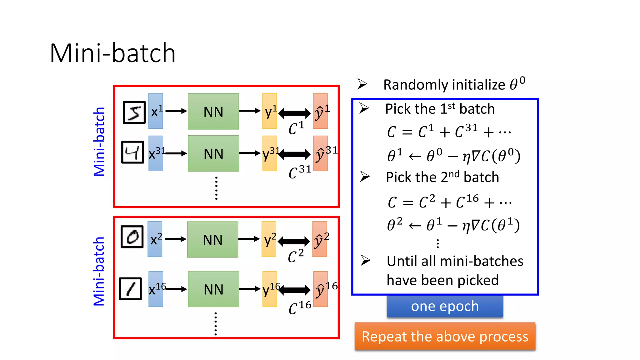
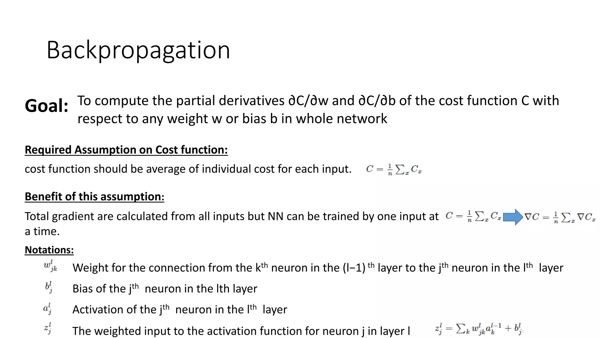
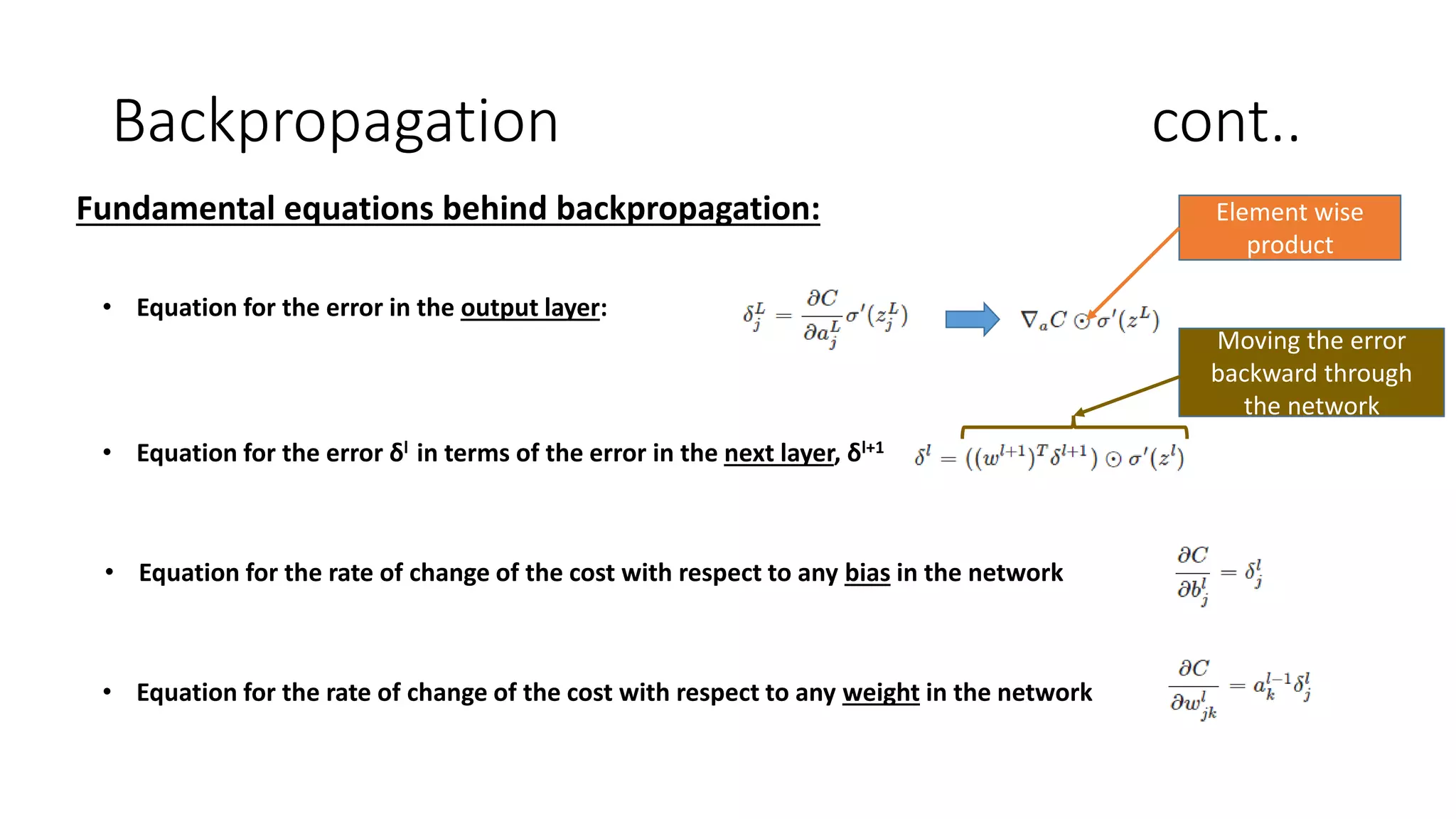
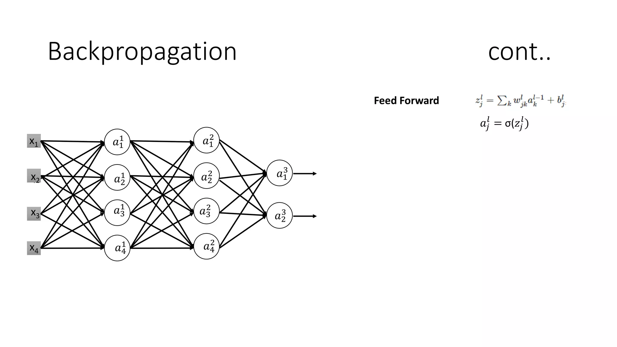
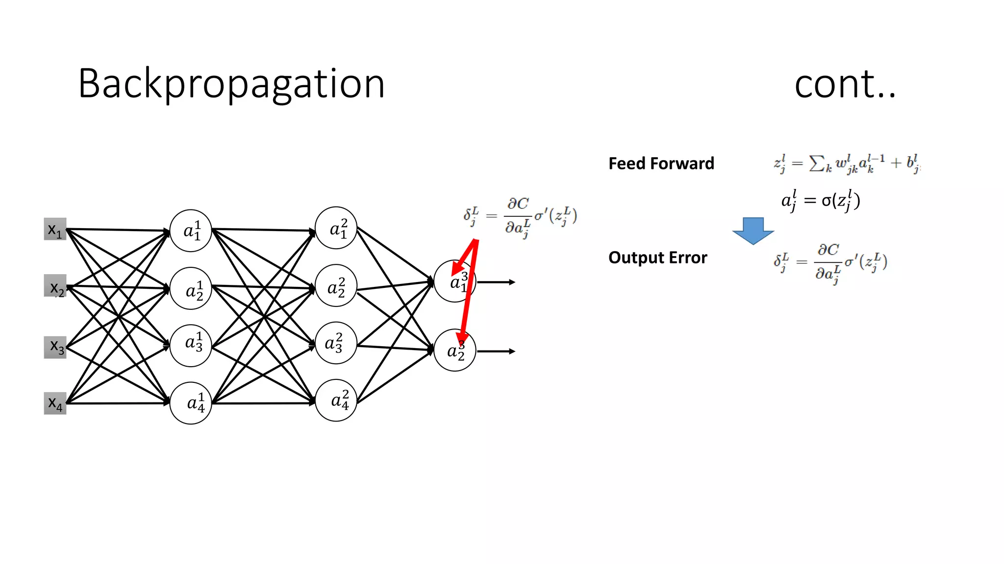
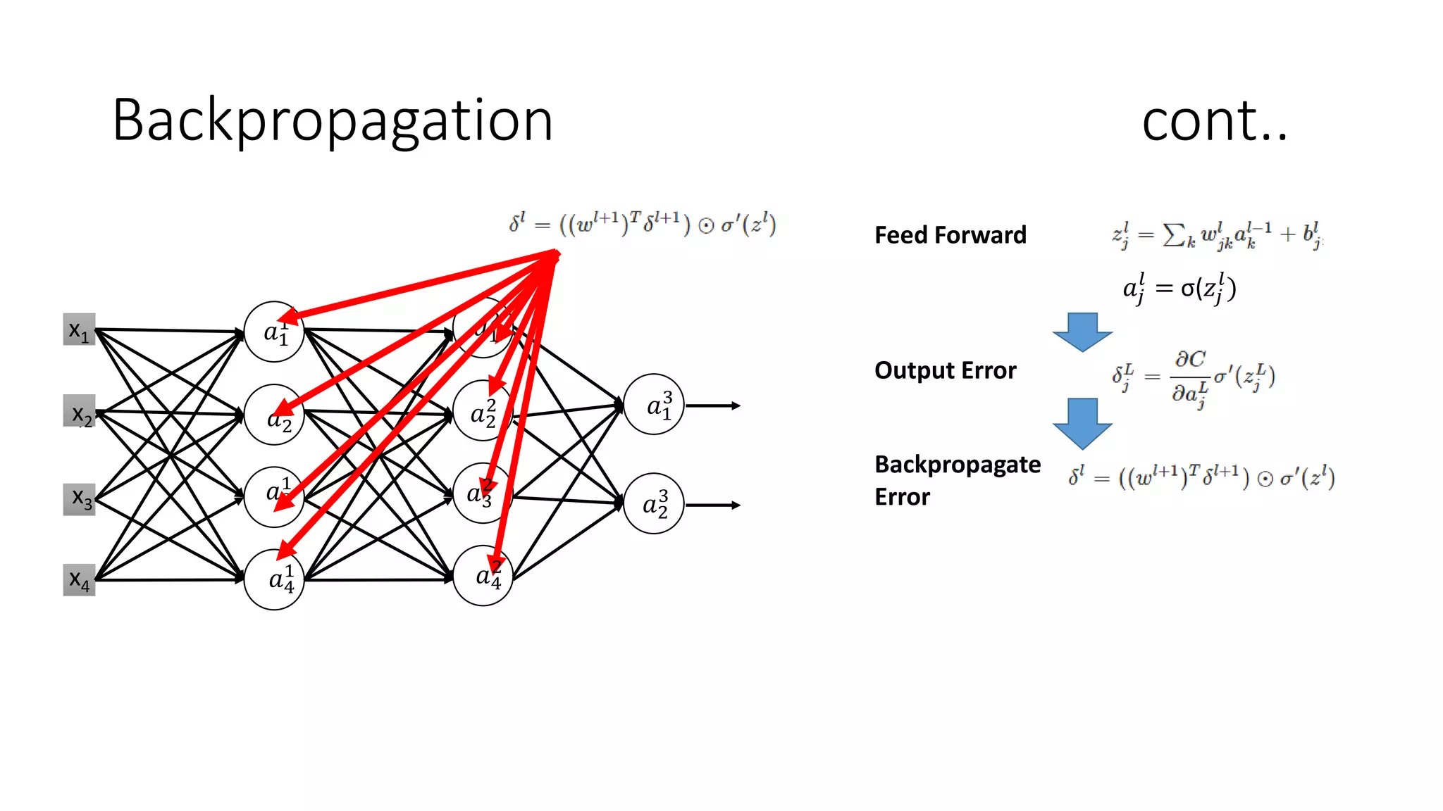
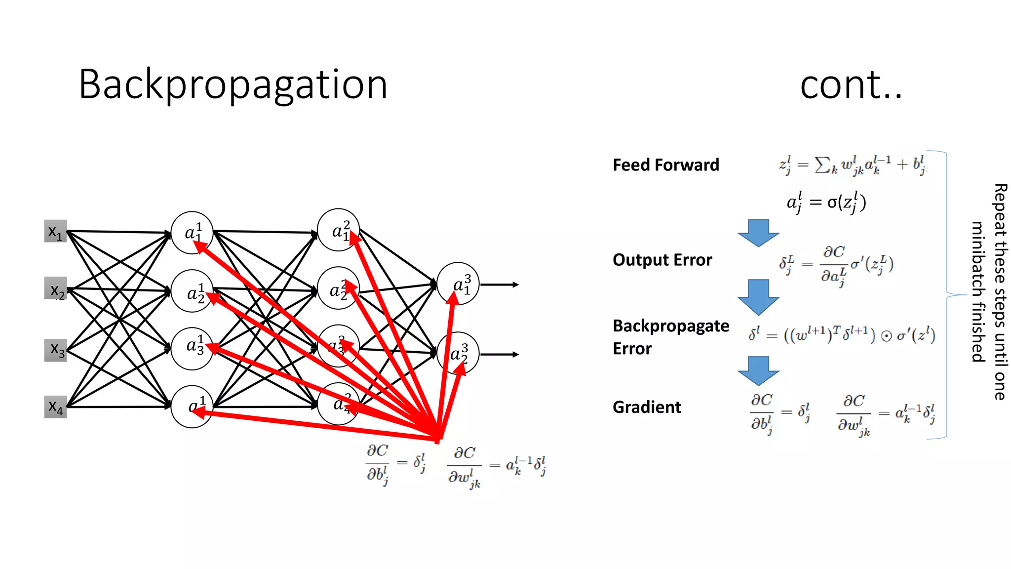
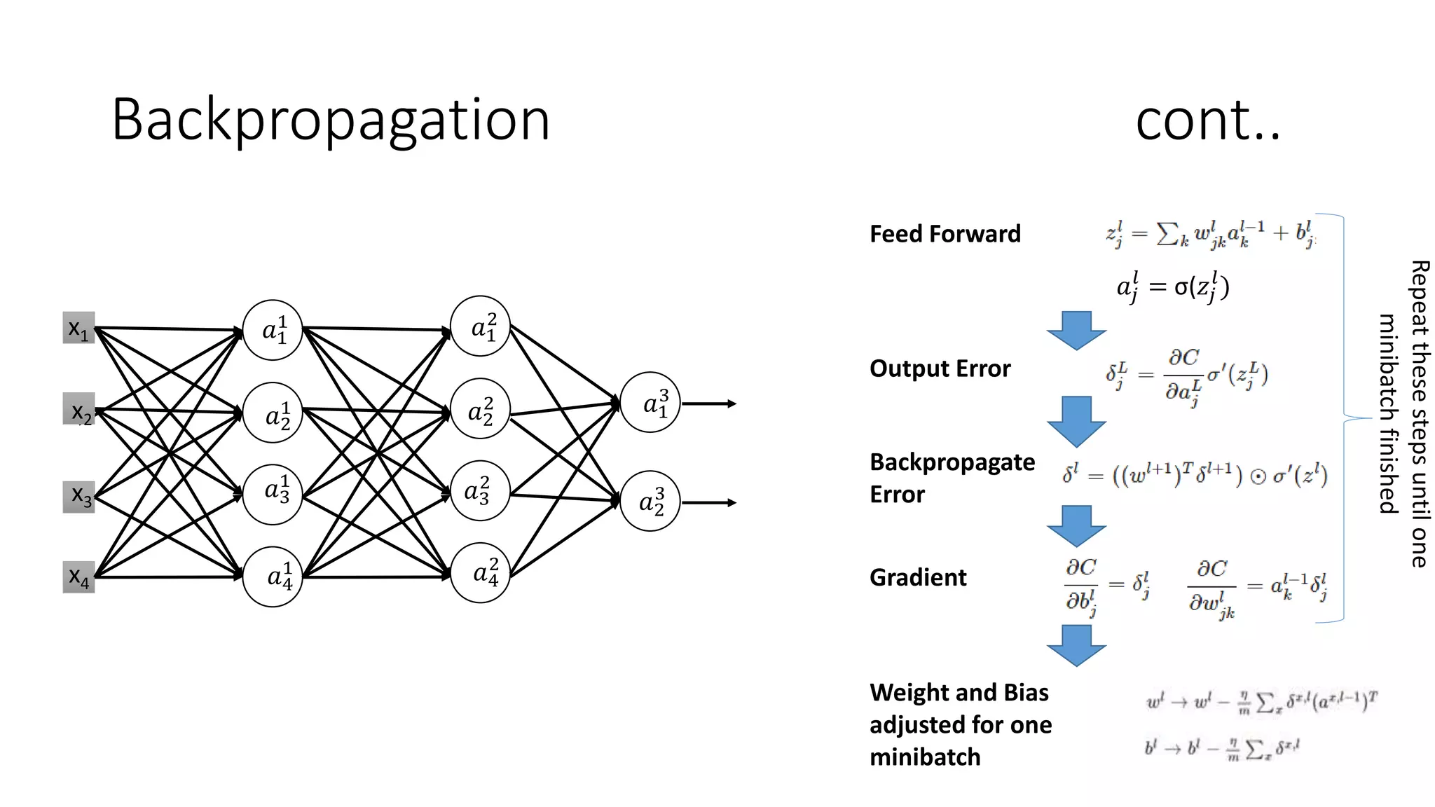
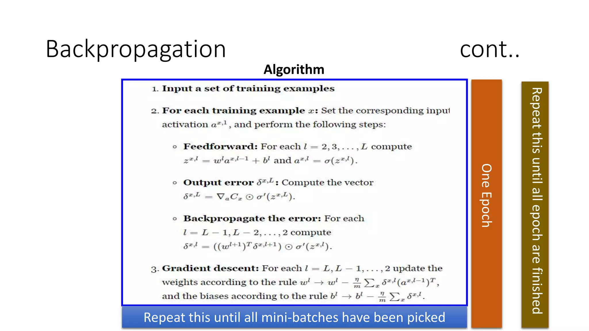
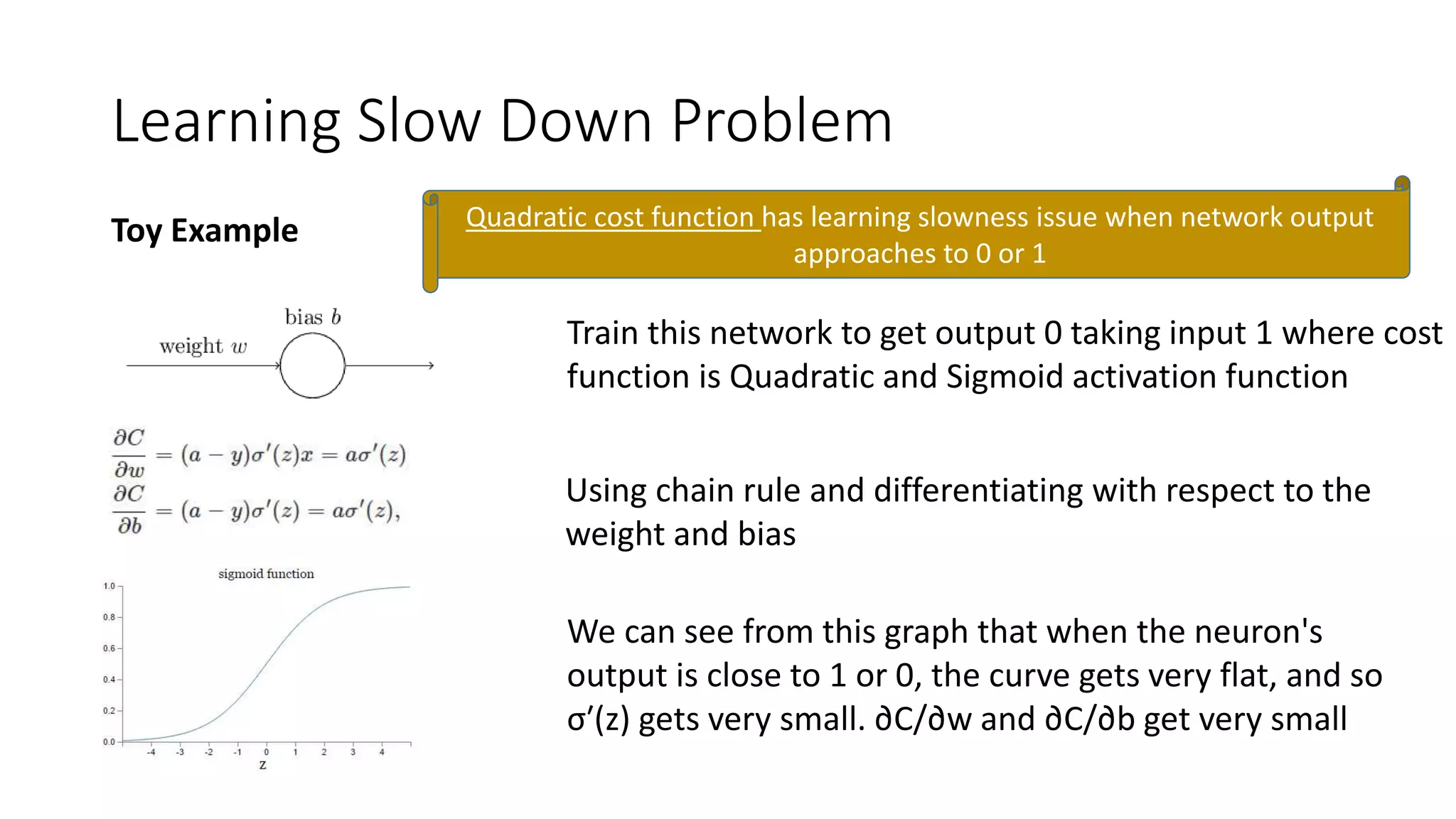
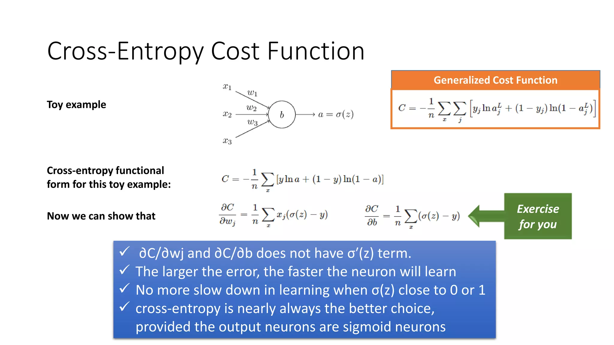
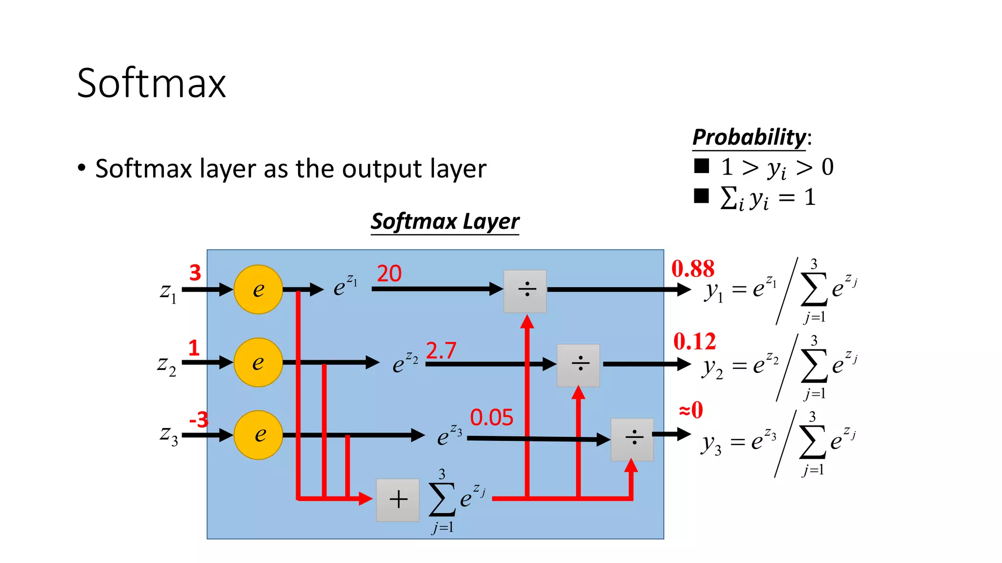
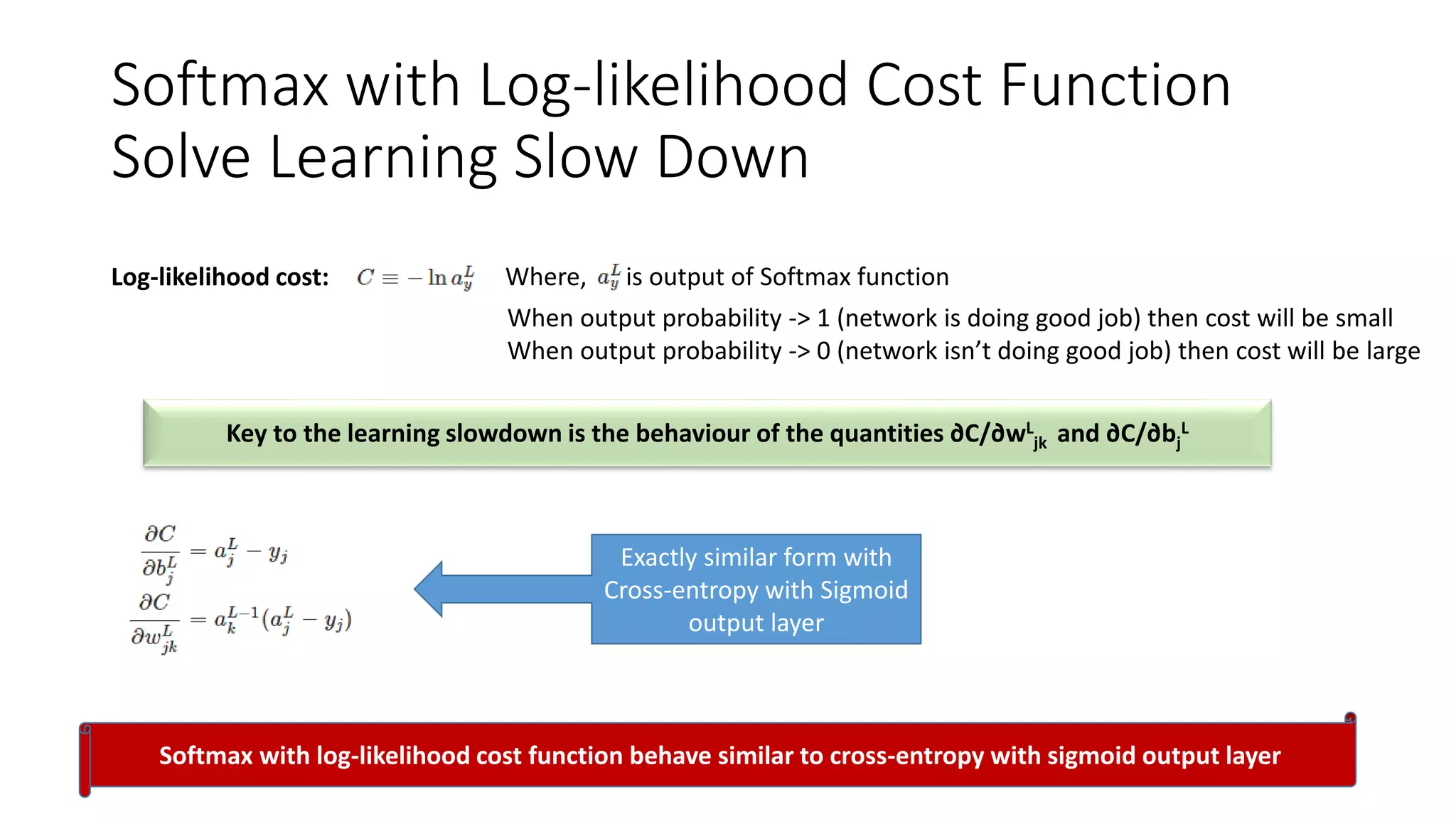
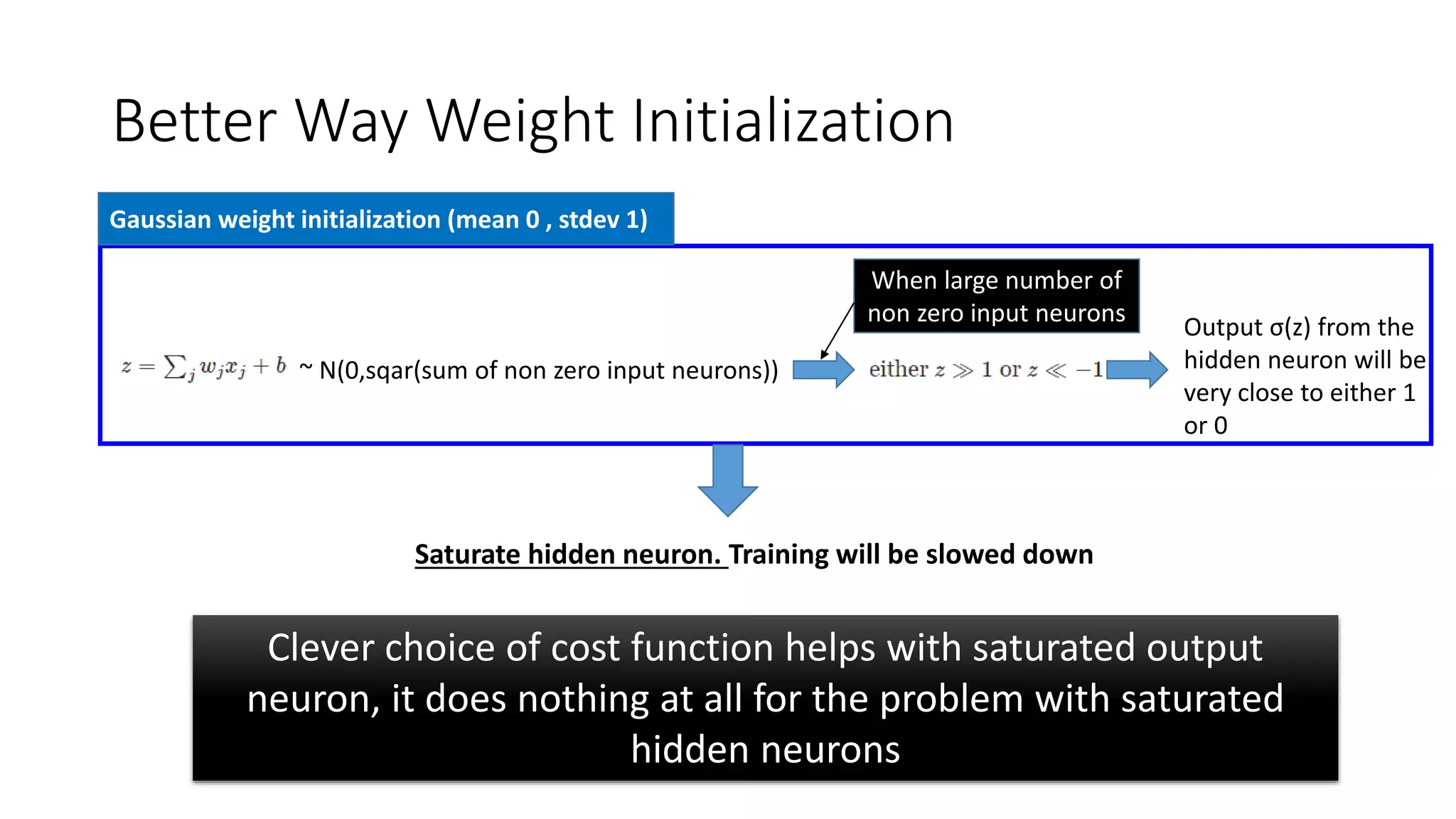
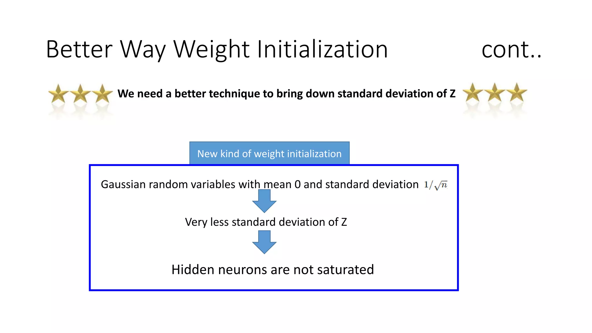
Neural network basic and introduction of Deep learning

Outline
Part IV: Tools and Technology to build CNN
Part III: Deep Learning
Part II: Improving the way neural networks learn
Part I: Introduction of Neural Network

Part I
Introduction of
Neural Network

Basic Approach
• Breaking big problem into many small task that computer can easily
perform
• In a neural network we don't tell the computer how to solve our
problem
• Instead, it learns from observational/training data, figuring out its
own solution (automatically infer rules) to the problem

Handwriting Digit Recognition(Propotype Problem)
Input Output
16 x 16 = 256
1x
2x
256x……
Ink → 1
No ink → 0
……
y1
y2
y10
Each dimension represents
the confidence of a digit.
is 1
is 2
is 0
……
0.1
0.7
0.2
The image
is “2”

Output
LayerHidden Layers
Input
Layer
Architecture of feedforward Neural Network
Input Output
1x
2x
Layer 1
……
Nx
……
Layer 2
……
Layer L
……
……
……
……
……
y1
y2
yM
Deep means many hidden layers
neuron

Artificial Neuron -- Perceptron
X1,x2,x3 are binary inputs
Produce binary output
Introduce weights on each inputs
Perceptron makes your decision by weighing up different factors/evidences
Here b = -threshold
b is called Bias

Learning Algorithm
• Automatically tune the weights and biases of a network
• Property: Small change in some weight (or bias) to cause only a small
corresponding change in the output
 Small change in the weights or bias of any
single perceptron in the network can
sometimes cause the output of that
perceptron to completely flip, say from 0 to 1
 This may classify one digit correctly but
completely wrong to classify other digits

Artificial Neuron -- Sigmoid
• Instead of input 0 or 1 it can take any value between 0 and 1
• Output can be between 0 and 1
• Sigmoid is the smoothed out perceptron
• Small change in weight and bias makes
small change in output – Achieved
• Function shape matters here so later we can think about other activation
function

Some Intuitive Explanation of NN
• Say input to neural network is
• Decide whether or not the digit is a 0 by weighing up evidence from
the hidden layer of neurons
• first neuron in the hidden layer detects
• Second neuron in the hidden layer detects
• Third neuron in the hidden layer detects
• Fourth neuron in the hidden layer detects
This is just a heuristically way to think about good neural network architecture
Classify

Cost Function
1x
2x
……
256x
……
……
……
……
……
y1
y2
y10
Cost
0.2
0.3
0.5
“1”
……
1
0
0
……
Lets start with quadratic cost function MSE
 Given a set of
network parameters
𝑤 and b, each
example has a cost
value
 Cost has to be
smooth function
 Small change in w
and b has to improve
in cost
target
C(𝑤, 𝑏)
Find the network parameters w and b that minimize the cost

Learning with Gradient Descent
𝑤1
𝑤2
Assume there are only two
parameters v1 and v2 in a
network.
The colors represent the value of C.
Randomly pick a starting point 𝜃0
Compute the gradient at 𝜃0
𝛻𝐶 𝜃0
𝜃0
𝛻𝐶 𝜃0
Amount of change in parameter
−𝜂𝛻𝐶 𝜃0
𝜃 = 𝑣1, 𝑣2
Cost Function Surface
𝜃∗
According to calculus
small of C for small change
in direction of v1 and v2
Parameter learning steps

Learning with Gradient Descent
𝑤1
𝑤2
𝜃0
𝜃1 𝛻𝐶 𝜃1
𝛻𝐶 𝜃2
𝜃2
Eventually, we would
reach a minima …..
Randomly pick a starting point 𝜃0
𝛻𝐶 𝜃0
Parameter learning steps
Compute the gradient at 𝜃0
Amount of change in parameter
Assume there are only two
parameters v1 and v2 in a
network. 𝜃 = 𝑣1, 𝑣2
According to calculus small
change of C due to small
change in direction of v1 and v2
Final formula for parameter
optimization

List of Further Improvements
• As mentioned earlier there are other type of cost functions
• Researcher came up with different forms of Gradient descent and
tried to introduce concept from physical world (i.e introducing
momentum)
• Many advancement happening on learning rate itself
• Came up with different techniques to initialize starting value of
parameters in Gradient descent
• Lot of improvements happened on neuron Activation function itself

Stochastic Gradient Descent
Where
High time
complexity when
huge sample size
Work around
Estimate the gradient ∇C by computing ∇Cx for a small sample
of randomly chosen training inputs
Mini-Batch

Mini-batch
x1
NN
……
y1
𝑦1
𝐶1
x31 NN y31
𝑦31
𝐶31
x2
NN
……
y2
𝑦2
𝐶2
x16 NN y16
𝑦16
𝐶16
 Pick the 1st batch
 Randomly initialize 𝜃0
𝜃1 ← 𝜃0 − 𝜂𝛻𝐶 𝜃0
 Pick the 2nd batch
𝜃2 ← 𝜃1 − 𝜂𝛻𝐶 𝜃1
 Until all mini-batches
have been picked
…
one epoch
Mini-batchMini-batch
Repeat the above process
𝐶 = 𝐶1 + 𝐶31 + ⋯
𝐶 = 𝐶2
+ 𝐶16
+ ⋯

Backpropagation
Goal: To compute the partial derivatives ∂C/∂w and ∂C/∂b of the cost function C with
respect to any weight w or bias b in whole network
Required Assumption on Cost function:
cost function should be average of individual cost for each input.
Benefit of this assumption:
Total gradient are calculated from all inputs but NN can be trained by one input at
a time.
Notations:
Weight for the connection from the kth neuron in the (l−1) th layer to the jth neuron in the lth layer
Bias of the jth neuron in the lth layer
Activation of the jth neuron in the lth layer
The weighted input to the activation function for neuron j in layer l

Backpropagation cont..
Fundamental equations behind backpropagation:
• Equation for the error in the output layer:
Element wise
product
• Equation for the error δl in terms of the error in the next layer, δl+1
Moving the error
backward through
the network
• Equation for the rate of change of the cost with respect to any bias in the network
• Equation for the rate of change of the cost with respect to any weight in the network

Feed Forward
𝑎𝑗
𝑙
= σ(𝑧𝑗
𝑙
)
𝑎1
1
𝑎2
1
𝑎3
1
𝑎4
1
𝑎1
2
𝑎2
2
𝑎3
2
𝑎4
2
𝑎1
3
𝑎2
3
x1
x2
x3
x4

Feed Forward
𝑎𝑗
𝑙
= σ(𝑧𝑗
𝑙
)
𝑎1
1
𝑎2
1
𝑎3
1
𝑎4
1
𝑎1
2
𝑎2
2
𝑎3
2
𝑎4
2
𝑎1
3
𝑎2
3
x1
x2
x3
x4
Output Error

𝑎1
1
𝑎2
1
𝑎3
1
𝑎4
1
𝑎1
2
𝑎2
2
𝑎3
2
𝑎4
2
𝑎1
3
𝑎2
3
x1
x2
x3
x4
Feed Forward
𝑎𝑗
𝑙
= σ(𝑧𝑗
𝑙
)
Output Error
Backpropagate
Error

Feed Forward
𝑎𝑗
𝑙
= σ(𝑧𝑗
𝑙
)
𝑎1
1
𝑎2
1
𝑎3
1
𝑎4
1
𝑎1
2
𝑎2
2
𝑎3
2
𝑎4
2
𝑎1
3
𝑎2
3
x1
x2
x3
x4
Output Error
Backpropagate
Error
Gradient
Repeatthesestepsuntilone
minibatchfinished

Feed Forward
𝑎𝑗
𝑙
= σ(𝑧𝑗
𝑙
)
𝑎1
1
𝑎2
1
𝑎3
1
𝑎4
1
𝑎1
2
𝑎2
2
𝑎3
2
𝑎4
2
𝑎1
3
𝑎2
3
x1
x2
x3
x4
Output Error
Backpropagate
Error
Gradient
Weight and Bias
adjusted for one
minibatch
Repeatthesestepsuntilone
minibatchfinished

Algorithm
Repeat this until all mini-batches have been picked
OneEpoch
Repeatthisuntilallepocharefinished

Exercise
1. Write a Python code to implement backpropagation algorithm as
mentioned in slide#24. You can download and use any suitable dataset for
parameter training.
2. Modify your code to remove loop mentioned in step# 2. Can we replace
this loop doing single matrix operation?

Part II:
Improving the Way Neural
Networks Learn

Learning Slow Down Problem
Toy Example
Train this network to get output 0 taking input 1 where cost
function is Quadratic and Sigmoid activation function
Using chain rule and differentiating with respect to the
weight and bias
We can see from this graph that when the neuron's
output is close to 1 or 0, the curve gets very flat, and so
σ′(z) gets very small. ∂C/∂w and ∂C/∂b get very small
Quadratic cost function has learning slowness issue when network output
approaches to 0 or 1

Cross-Entropy Cost Function
Cross-entropy functional
form for this toy example:
Toy example
Now we can show that
 ∂C/∂wj and ∂C/∂b does not have σ′(z) term.
 The larger the error, the faster the neuron will learn
 No more slow down in learning when σ(z) close to 0 or 1
 cross-entropy is nearly always the better choice,
provided the output neurons are sigmoid neurons
Exercise
for you
Generalized Cost Function

Exercise
Show that slowness problem can be resolved if we use linear
neurons in the output layer even if we use quadratic cost
function and sigmoid activation in all internal neurons.

Softmax
• Softmax layer as the output layer
1z
2z
3z
Softmax Layer
e
e
e
1z
e
2z
e
3z
e



3
1
1
1
j
zz j
eey

3
1j
z j
e



3
-3
1 2.7
20
0.05
0.88
0.12
≈0
Probability:
 1 > 𝑦𝑖 > 0
 𝑖 𝑦𝑖 = 1


3
1
2
2
j
zz j
eey


3
1
3
3
j
zz j
eey

Softmax with Log-likelihood Cost Function
Solve Learning Slow Down
Log-likelihood cost: Where, is output of Softmax function
When output probability -> 1 (network is doing good job) then cost will be small
When output probability -> 0 (network isn’t doing good job) then cost will be large
Key to the learning slowdown is the behaviour of the quantities ∂C/∂wL
jk and ∂C/∂bj
L
Exactly similar form with
Cross-entropy with Sigmoid
output layer
Softmax with log-likelihood cost function behave similar to cross-entropy with sigmoid output layer

Exercise
Implement backpropagation with Softmax and the log-likelihood
cost function in python

Overfitting Problem
• Training data accuracy increases as we increase number of epochs on fix network
architecture and fixed training dataset but Test data accuracy reaches in
saturation after some time
• Complex network with many parameters but not adequate training examples
General Strategy to overcome overfitting
 Increase training data size
 Reduce network size
 Use validation set to determine best hyper parameter settings
Observe Overfitting issue

Regularization
Regularization can reduce overfitting, even when we have a fixed network and fixed training
data. It helps to resist to learn errors in the training data and only learn common patterns
L2 regularization
L1 regularization
Dropout
• Modify cost function and force network weight
parameters not to increase too much due to some
peculiarities in the training data
• Add only weight rescaling factor in the learning rule
Dropout doesn't rely on modifying the cost function. Instead, it modifies the
network itself.
Artificially increasing the training set size Introduce small amount of distortion in training data to increase total
size. Like small rotation of image, include background noise in the
speech data

Dropout
Training:
𝜃 𝑡 ← 𝜃 𝑡−1 − 𝜂𝛻𝐶 𝜃 𝑡−1
 Each time before computing the gradients
 Each neuron has p% to dropout
Pick a mini-batch

Dropout
Training:
 Each time before computing the gradients
 Each neuron has p% to dropout
 Using the new network for training
The structure of the network is changed.
Thinner!
For each mini-batch, we resample the dropout neurons
𝜃 𝑡 ← 𝜃 𝑡−1 − 𝜂𝛻𝐶 𝜃 𝑡−1
Pick a mini-batch

Dropout
Testing:
 No dropout
 If the dropout rate at training is p%,
all the weights times (1-p)%
 Assume that the dropout rate is 50%.
If a weight w = 1 by training, set 𝑤 = 0.5 for testing.

Dropout - Intuitive Reason
 When teams up, if everyone expect the partner will do
the work, nothing will be done finally.
 However, if you know your partner will dropout, you
will do better.
My partner will
put bad , so I
was going to do
 When testing, no one dropout actually, so obtaining
good results eventually.

Dropout - Intuitive Reason
• Why the weights should multiply (1-p)% (dropout rate) when testing?
Training of Dropout Testing of Dropout
𝑤1
𝑤2
𝑤3
𝑤4
𝑧
𝑤1
𝑤2
𝑤3
𝑤4
𝑧′
Assume dropout rate is 50%
0.5 ×
0.5 ×
0.5 ×
0.5 ×
No dropout
Weights from training
𝑧′ ≈ 2𝑧
𝑧′ ≈ 𝑧
Weights multiply (1-p)%

Dropout is a kind of ensemble.
Ensemble
Network
1
Network
2
Network
3
Network
4
Train a bunch of networks with different structures
Training
Set
Set 1 Set 2 Set 3 Set 4

Ensemble
y1
Network
1
Network
2
Network
3
Network
4
Testing data x
y2 y3 y4
average

Training of
Dropout
minibatch
1
……
Using one mini-batch to train one network
Some parameters in the network are shared
minibatch
2
minibatch
3
minibatch
4
M neurons
2M possible
networks

testing data x
Testing of Dropout
……average
y1 y2 y3
All the
weights
multiply
(1-p)%
≈ y

Better Way Weight Initialization
~ N(0,sqar(sum of non zero input neurons))
When large number of
non zero input neurons
Output σ(z) from the
hidden neuron will be
very close to either 1
or 0
Saturate hidden neuron. Training will be slowed down
Clever choice of cost function helps with saturated output
neuron, it does nothing at all for the problem with saturated
hidden neurons
Gaussian weight initialization (mean 0 , stdev 1)

Better Way Weight Initialization cont..
We need a better technique to bring down standard deviation of Z
New kind of weight initialization
Gaussian random variables with mean 0 and standard deviation
Very less standard deviation of Z
Hidden neurons are not saturated

How to choose a neural network's Hyper-
Parameters?

Why Deep Learning?
• Deep network increase accuracy
• It breaks down complex question into very simple questions. It does this through
series of many layers
• It modularizes classification task

Why Deep Network Hard to Train?
Vanishing gradient problem
Deep Network- Toy example
Weight initialized by Gaussian with
mean 0 and standard deviation 1
1.
2.
3.
16 times smaller
Neurons in the
earlier layers learn
much more slowly
than neurons in later
layers
1.
2.
3.

Convolutional Neural Network (CNN)
Three basic ideas
 local receptive fields
 shared weights
 Pooling
It won't connect every input pixel to every hidden neuron. Instead, it only
makes connections in small, localized regions of the input image
It uses the same weight and bias for each of the hidden neurons in a
particular hidden layer
Simplify the information in the output from the convolutional layer

Local Receptive Fields
• Hidden neuron connects to small, localized region of the input neurons
local receptive
field
length of shift of Local receptive field window to create hidden neuronsStride length:

Shared Weights and Biases
• Share same set of weights and bias for each local receptive fields windows
Activation value of j,k th hidden neuron
Where, local receptive field
window size 5 X 5
• All the neurons in the one hidden layer detect exactly the same feature, just at
different location of input data
• Shared weights and bias are often said to define a kernel or filter
• Map from the input layer to the hidden layer is call a feature map
• Multiple feature maps forms the convolutional layer

Pooling Layer
• Pooling layers are usually used immediately after convolutional layers
• Pooling layer takes each feature map output from the convolutional layer and
prepares a condensed feature map
• One common procedure for pooling is known as max-pooling. simply outputs the
maximum activation in given input region
• This helps reduce the number of parameters needed in later layers

Basic Architecture of CNN
Input
neurons
Feature
map
Fully connected
network

Tips for Training CNN
• Use Rectified linear units (ReLU) instead of Sigmoid activation function (handle
vanishing gradient problem)
• Expand training data introducing some distortion, rotation, shift, background noise etc.
• Try with introducing extra convolutional-pooling layers
• Inserting an extra fully-connected layer
• Use dropout regularization to the fully-connected layers

Part IV
Tools and Technology to
build CNN

Open Source Libraries
• Machine learning library Theano
-- it has implementation of backpropagation of CNN, dropout like all useful
components to build CNN
-- it can run code on either a CPU or, if available, a NVIDIA GPU
• CAFFE
• Deeplearning4J
• Torch

Exercise
Install Caffe after installing NVDIA driver and Cuda platform in your machine. Then run
Alexnet CNN model in GPU mode.

Neural network basic and introduction of Deep learning

More Related Content

What's hot

Similar to Neural network basic and introduction of Deep learning

Recently uploaded

Neural network basic and introduction of Deep learning

Editor's Notes