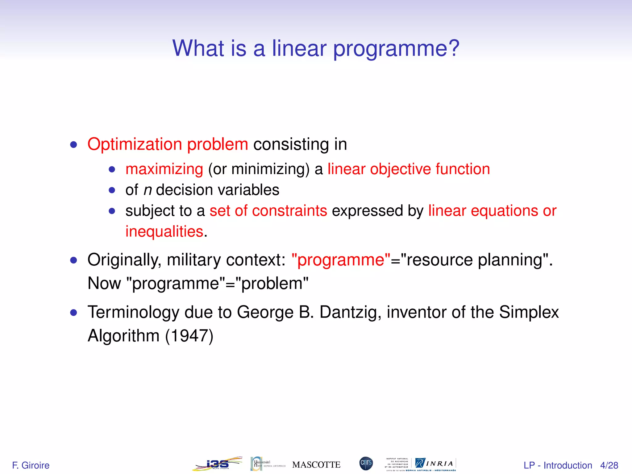
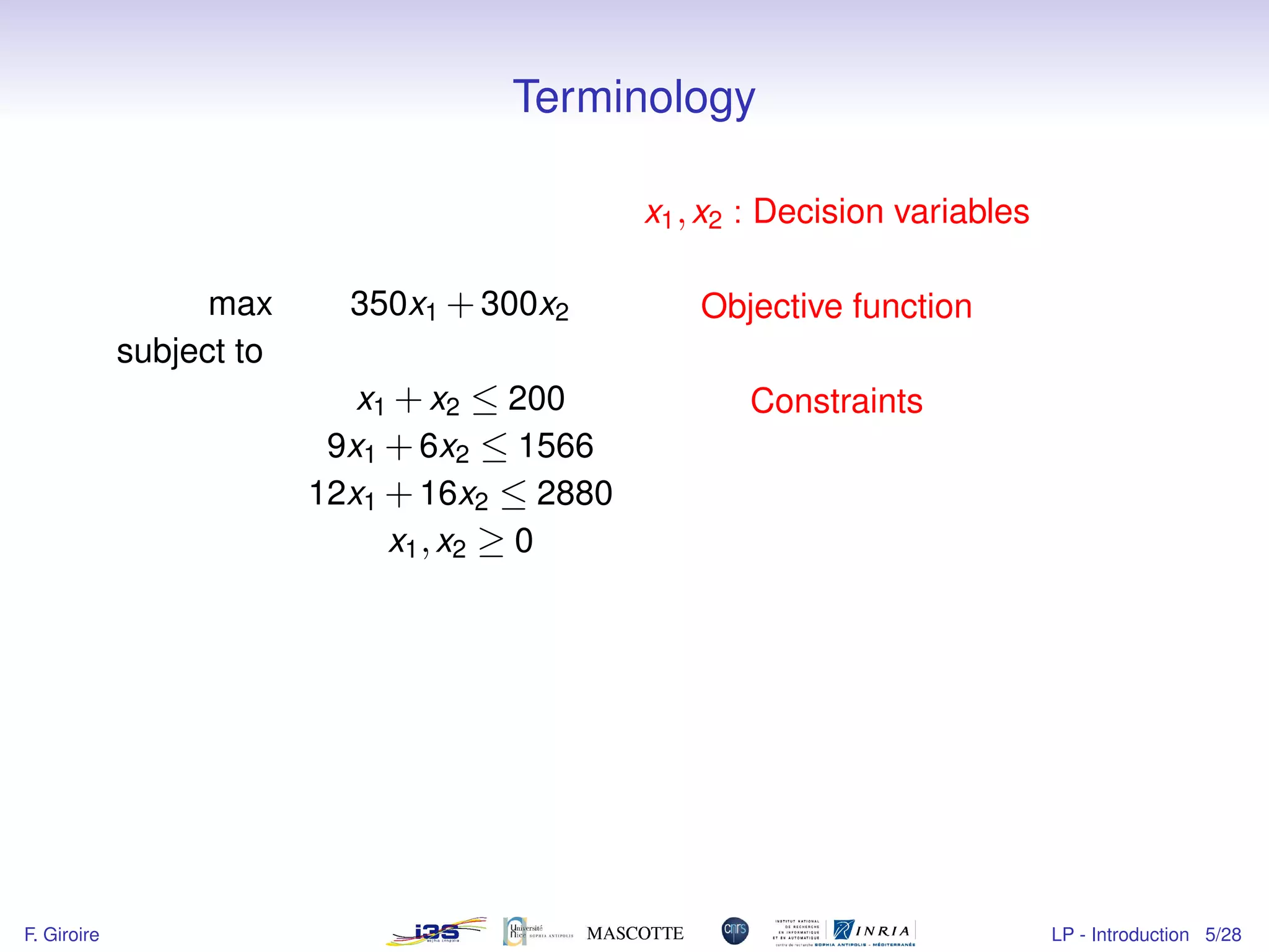
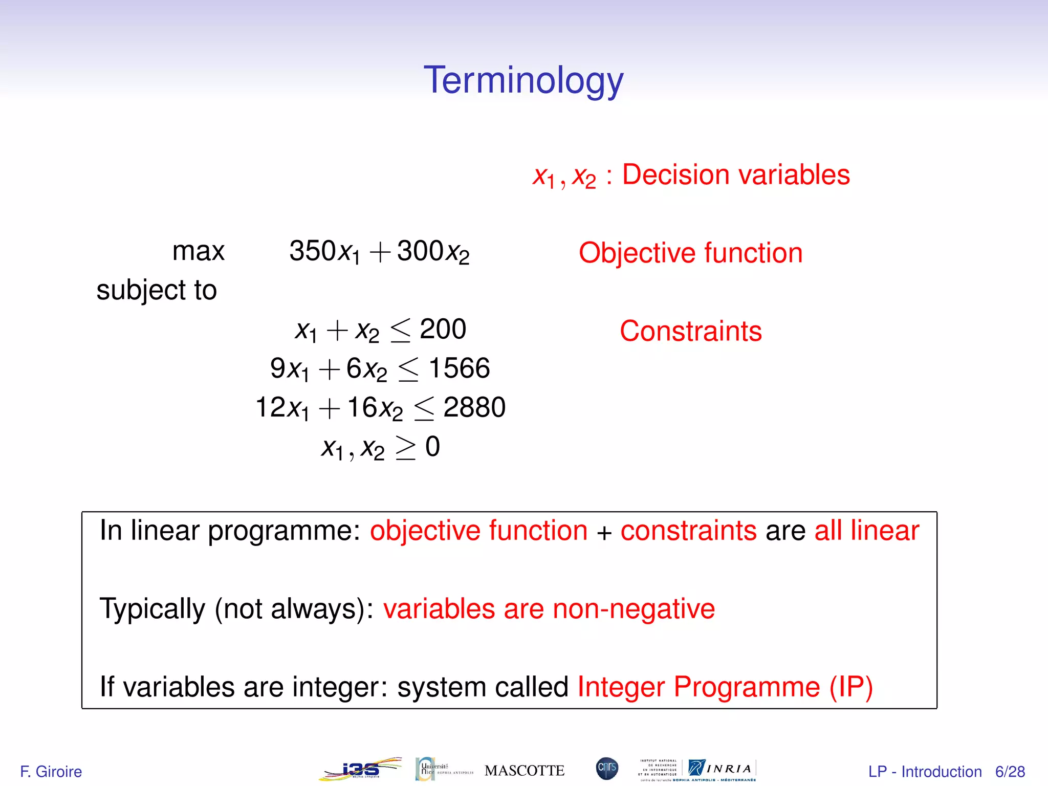
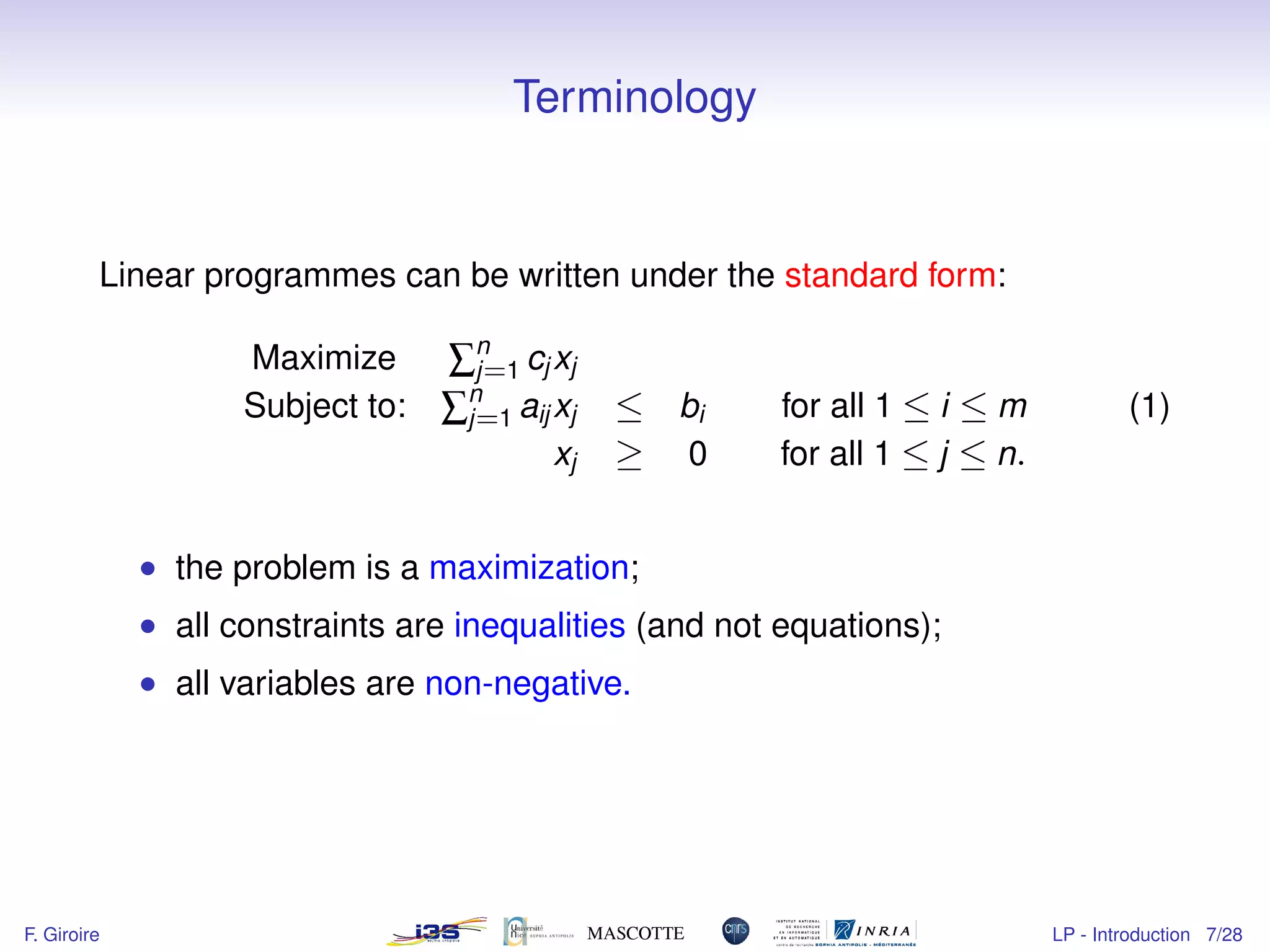
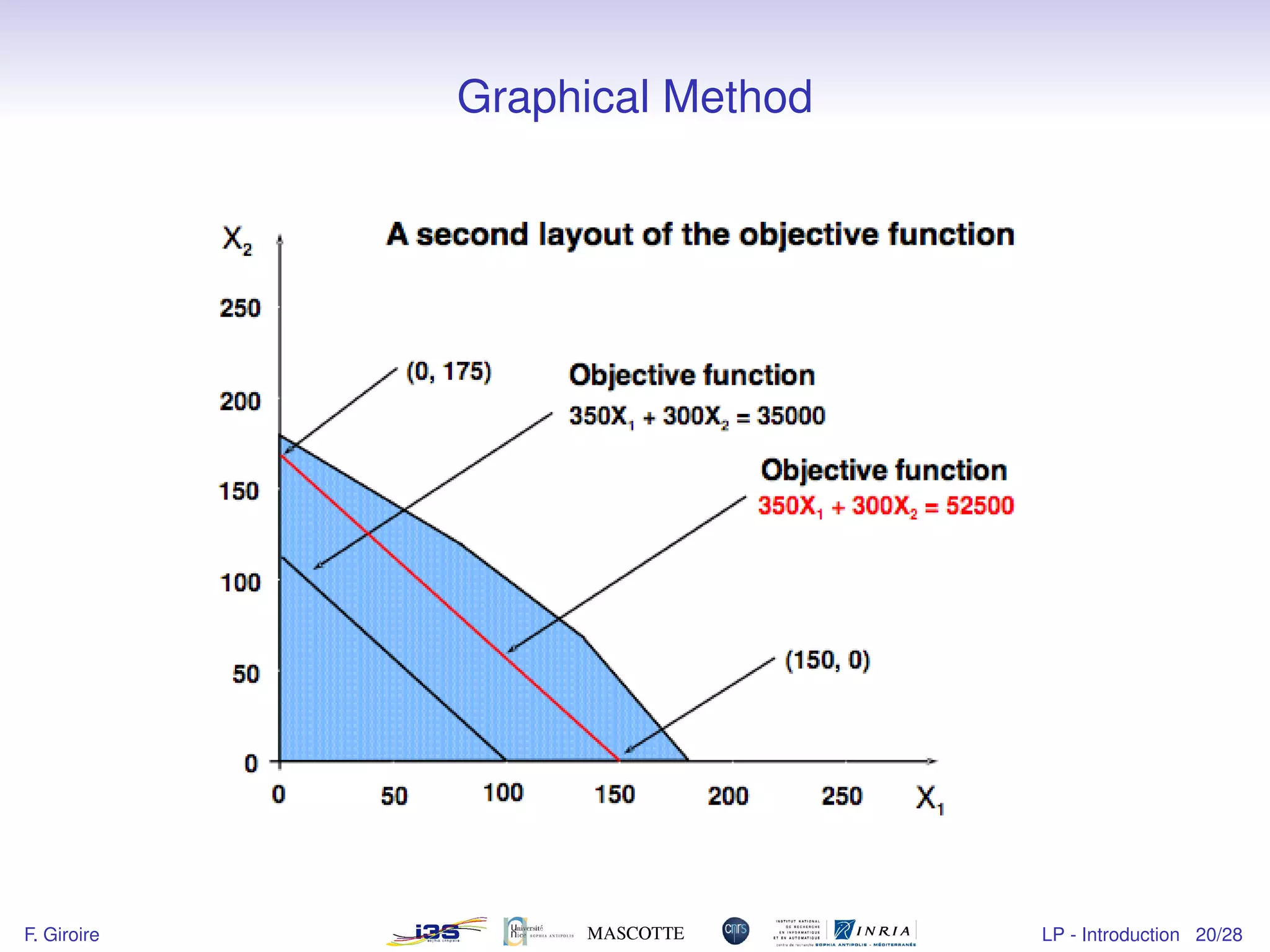
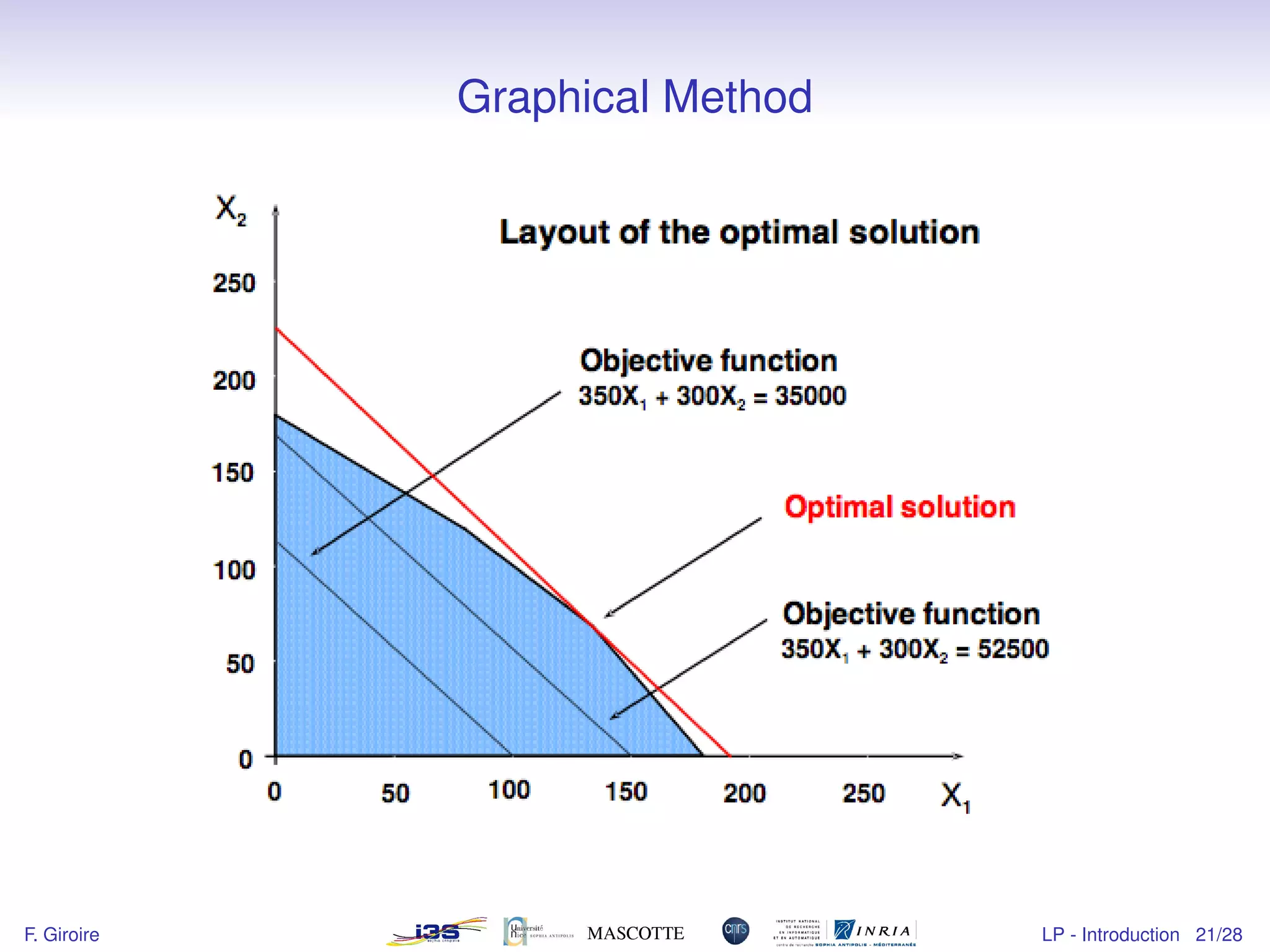
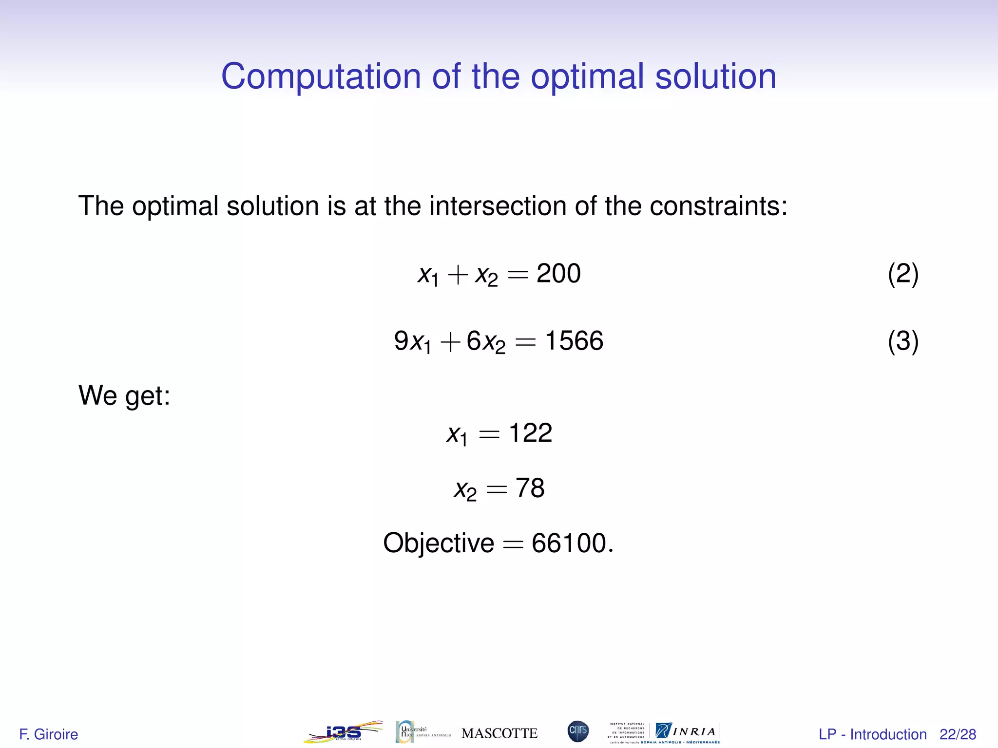
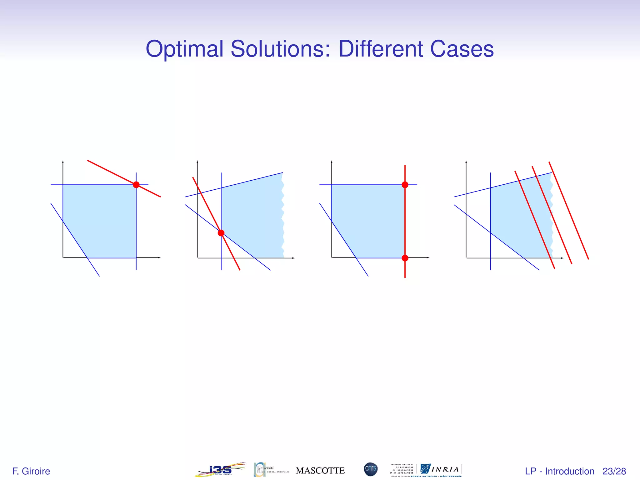
1) The document introduces linear programming, which involves optimizing a linear objective function subject to linear constraints.
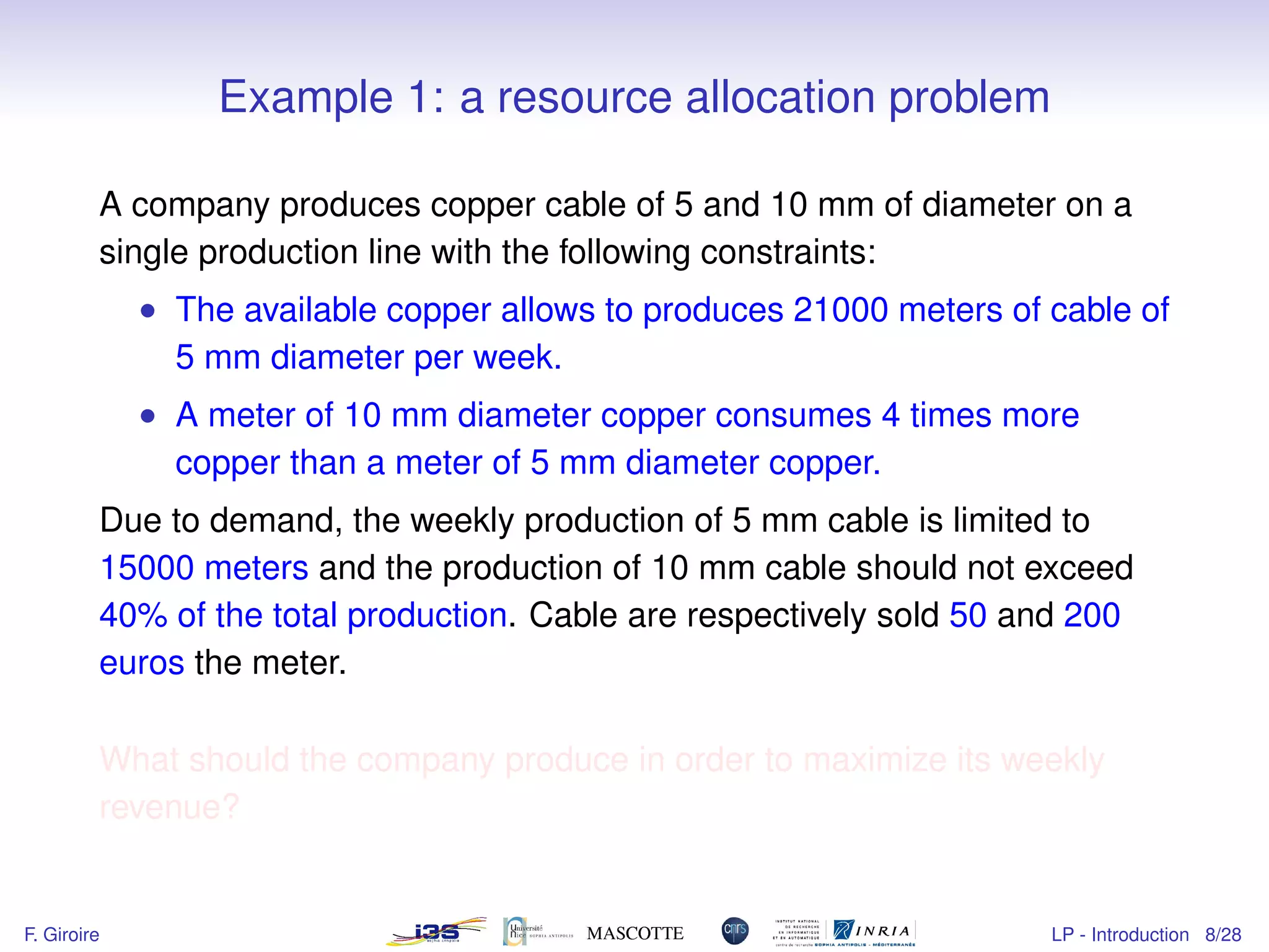
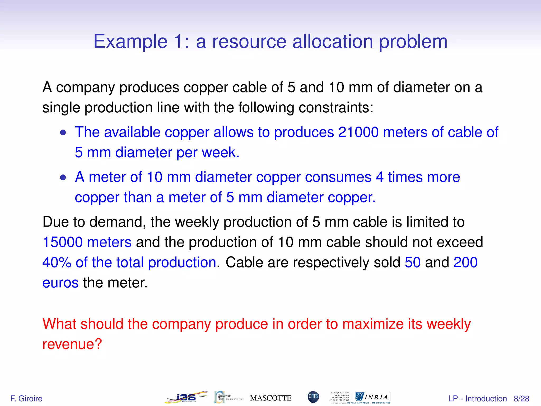
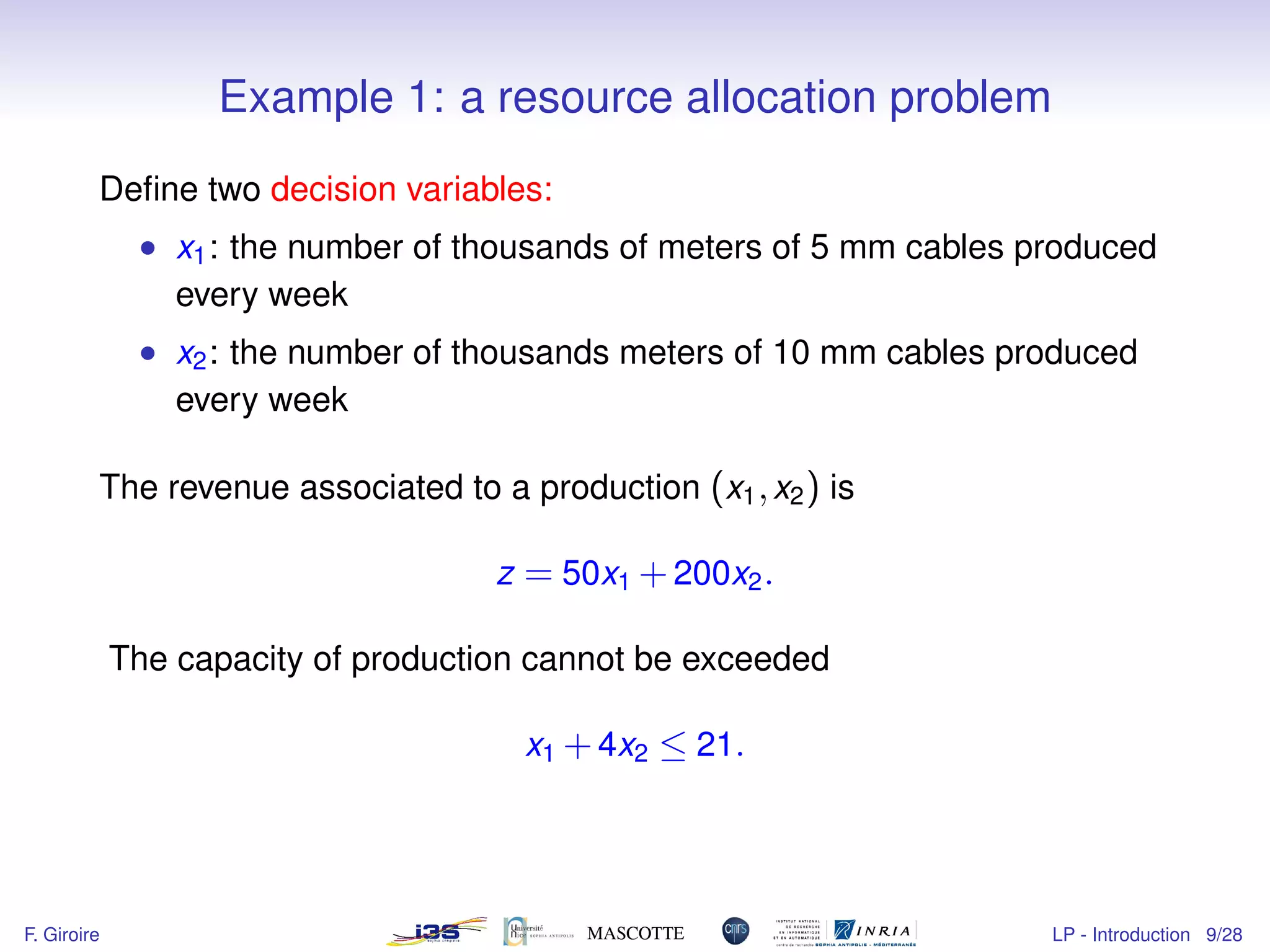
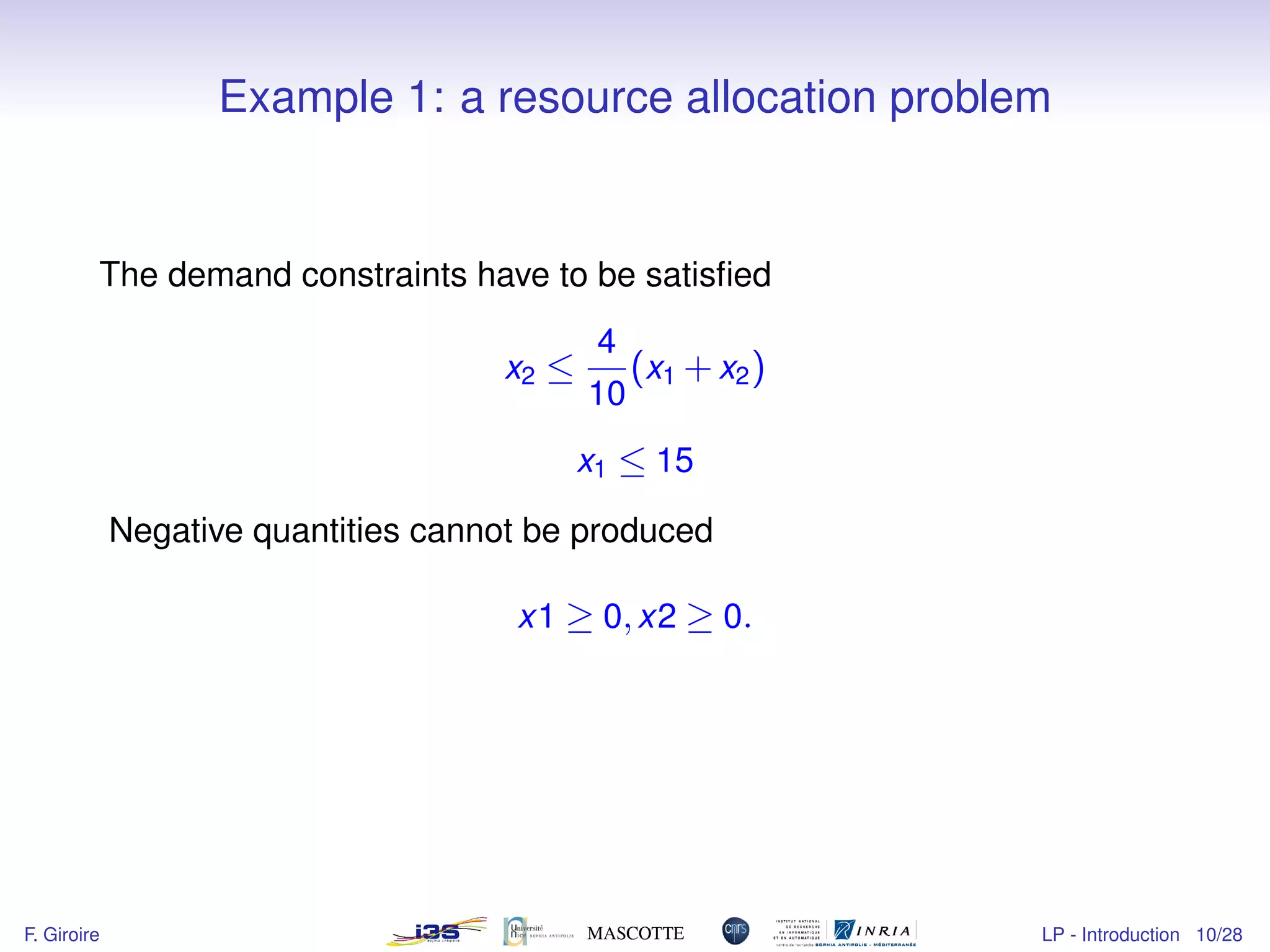
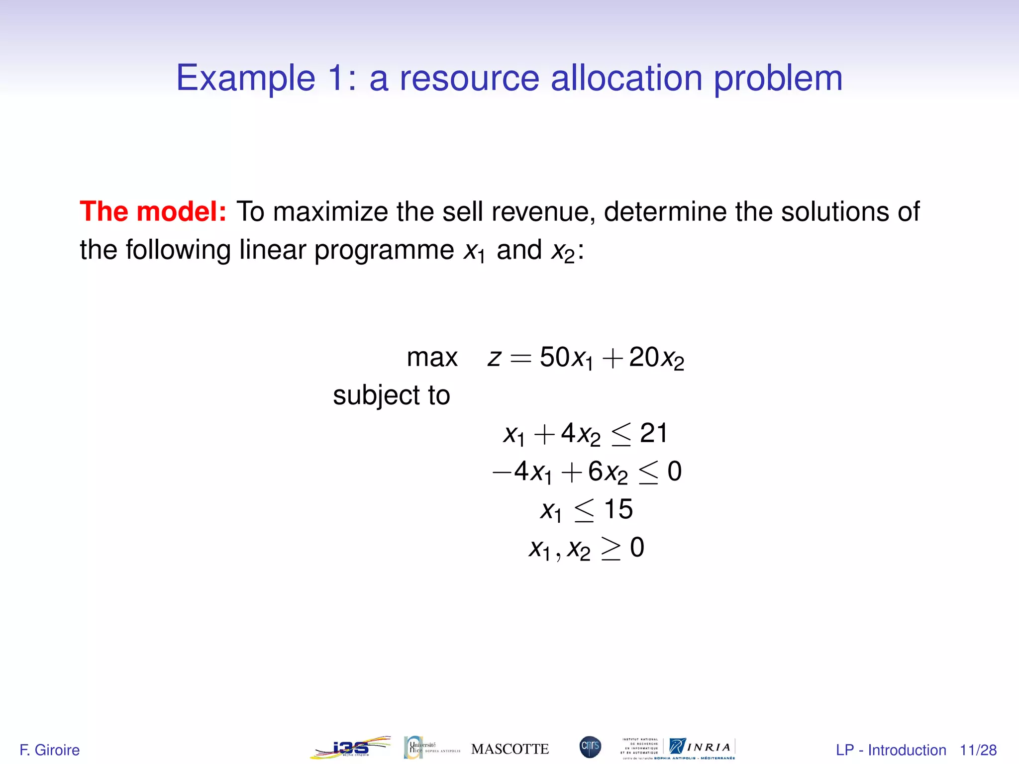
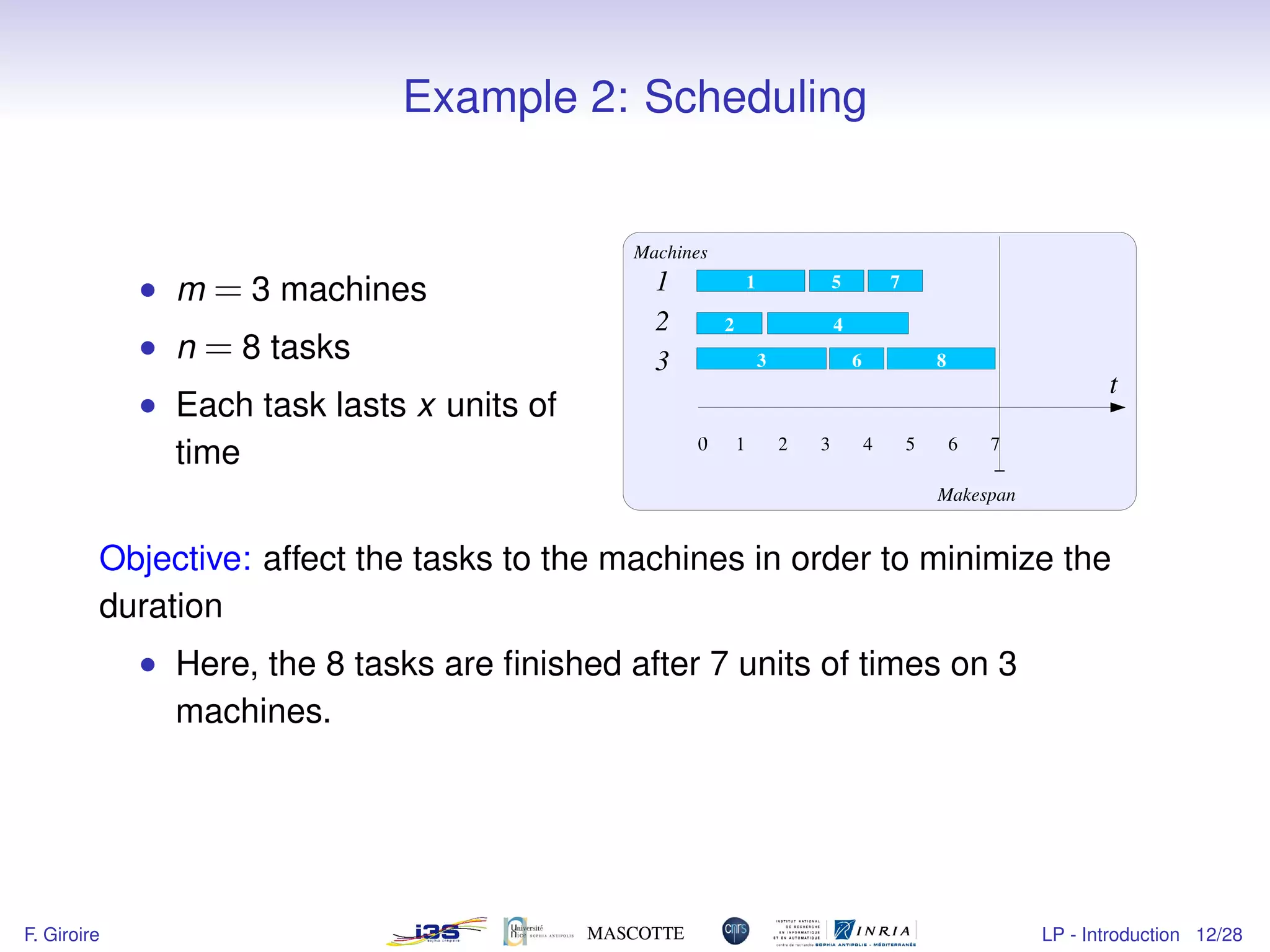
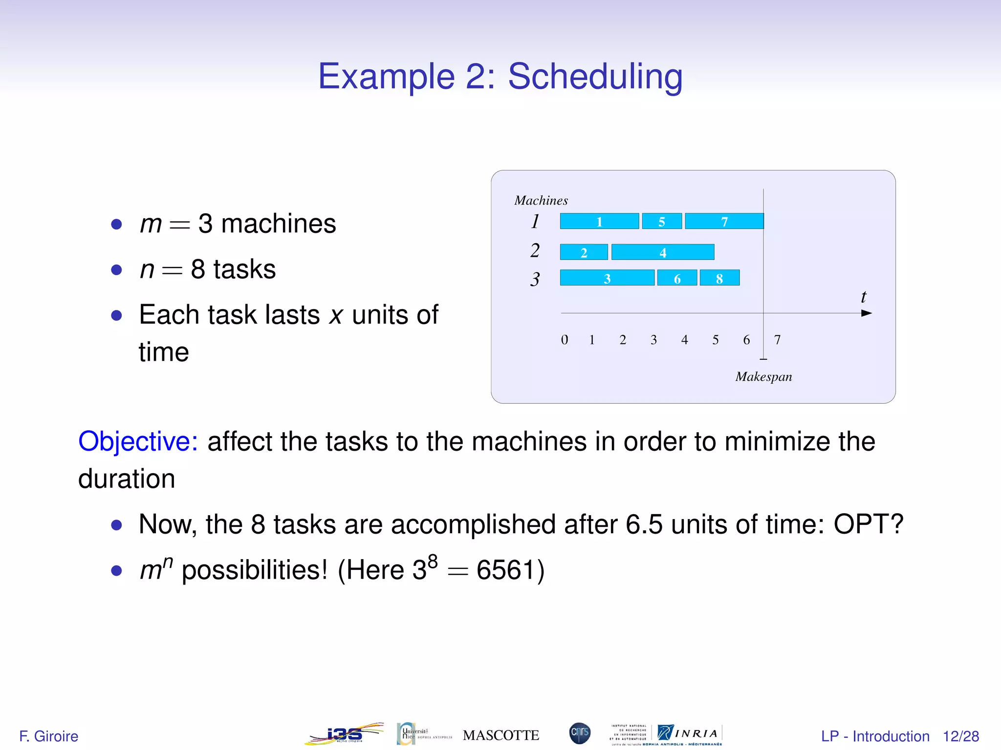
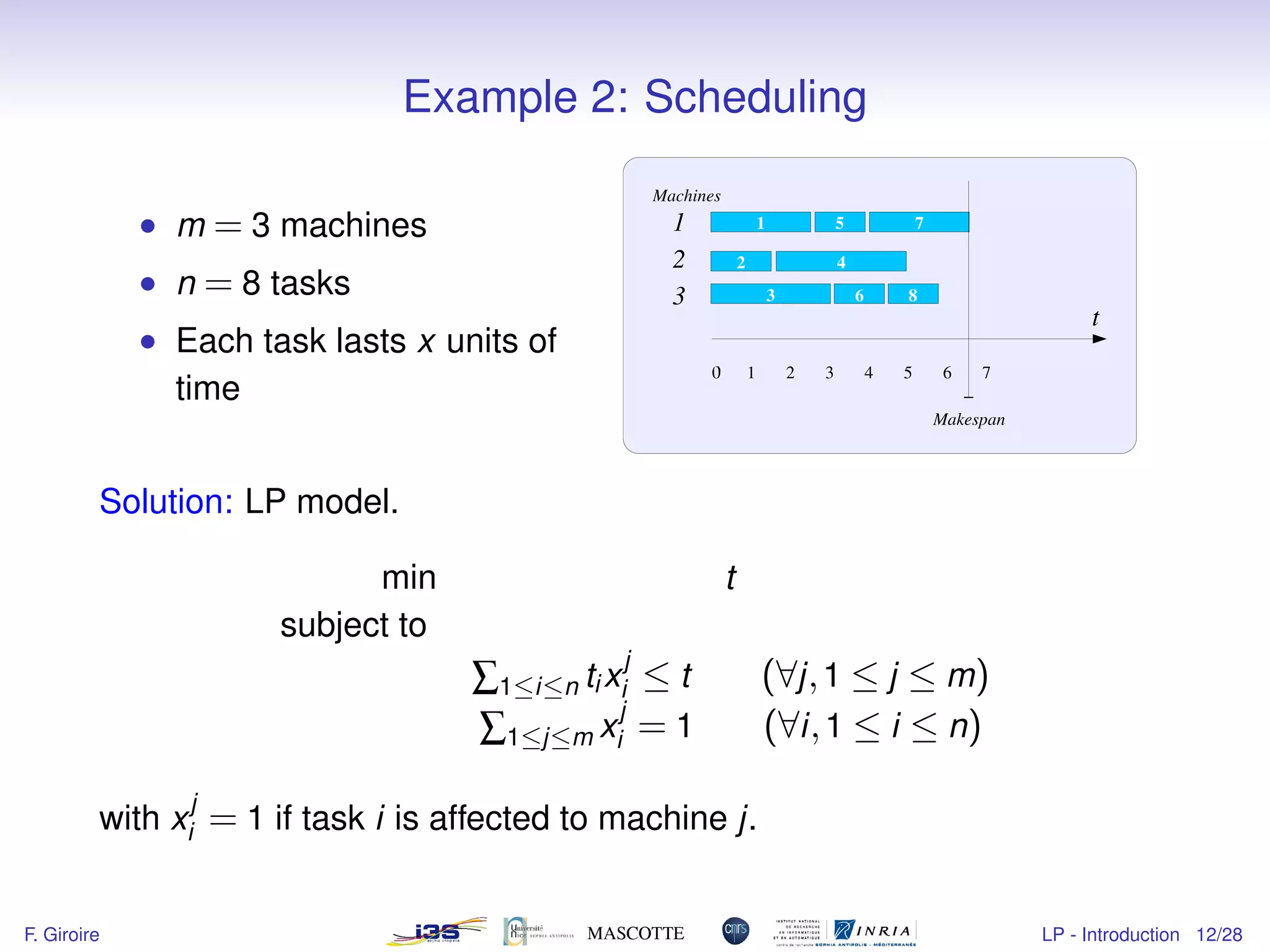
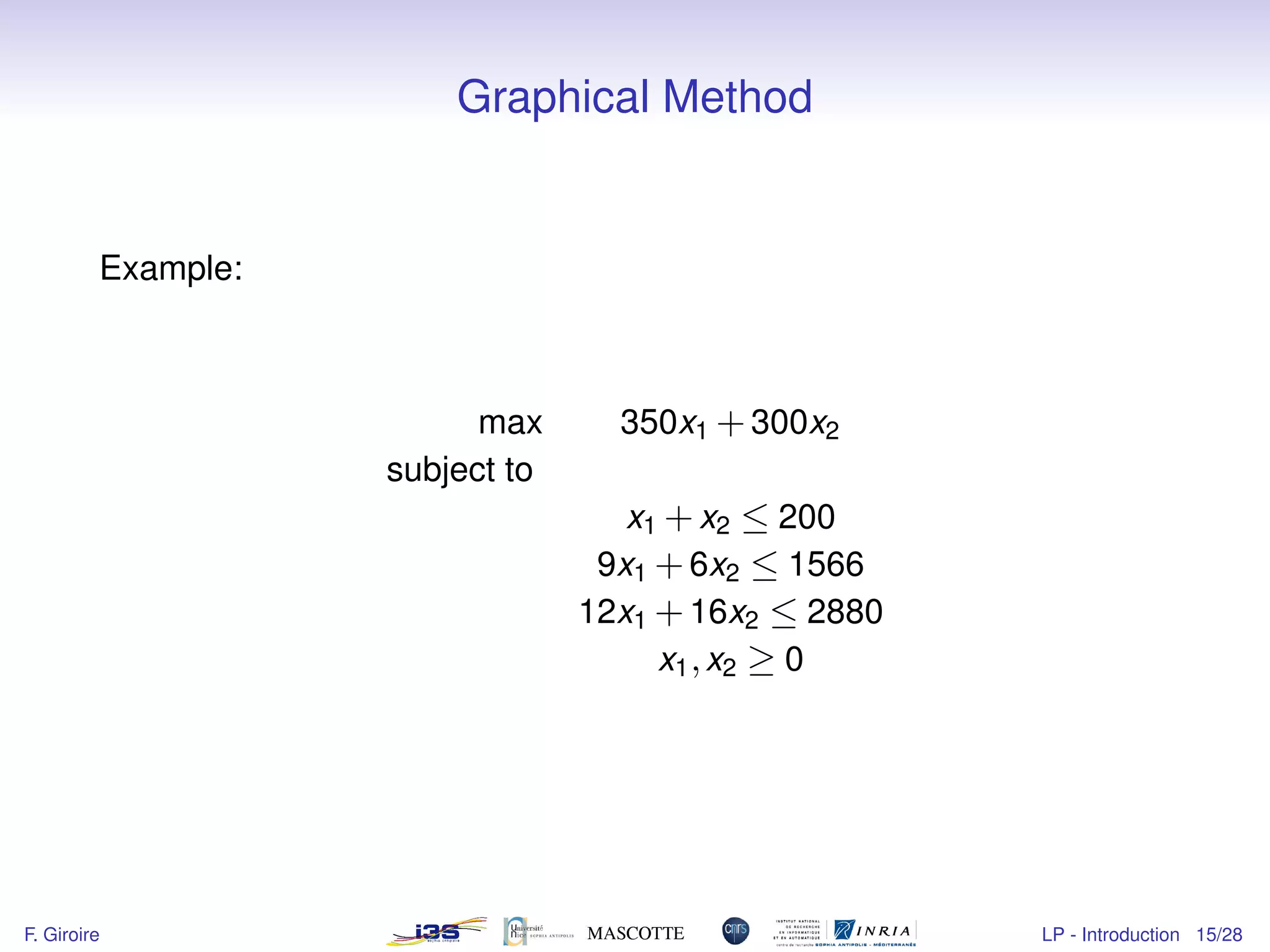
2) It provides examples of resource allocation and scheduling problems that can be modeled as linear programs.
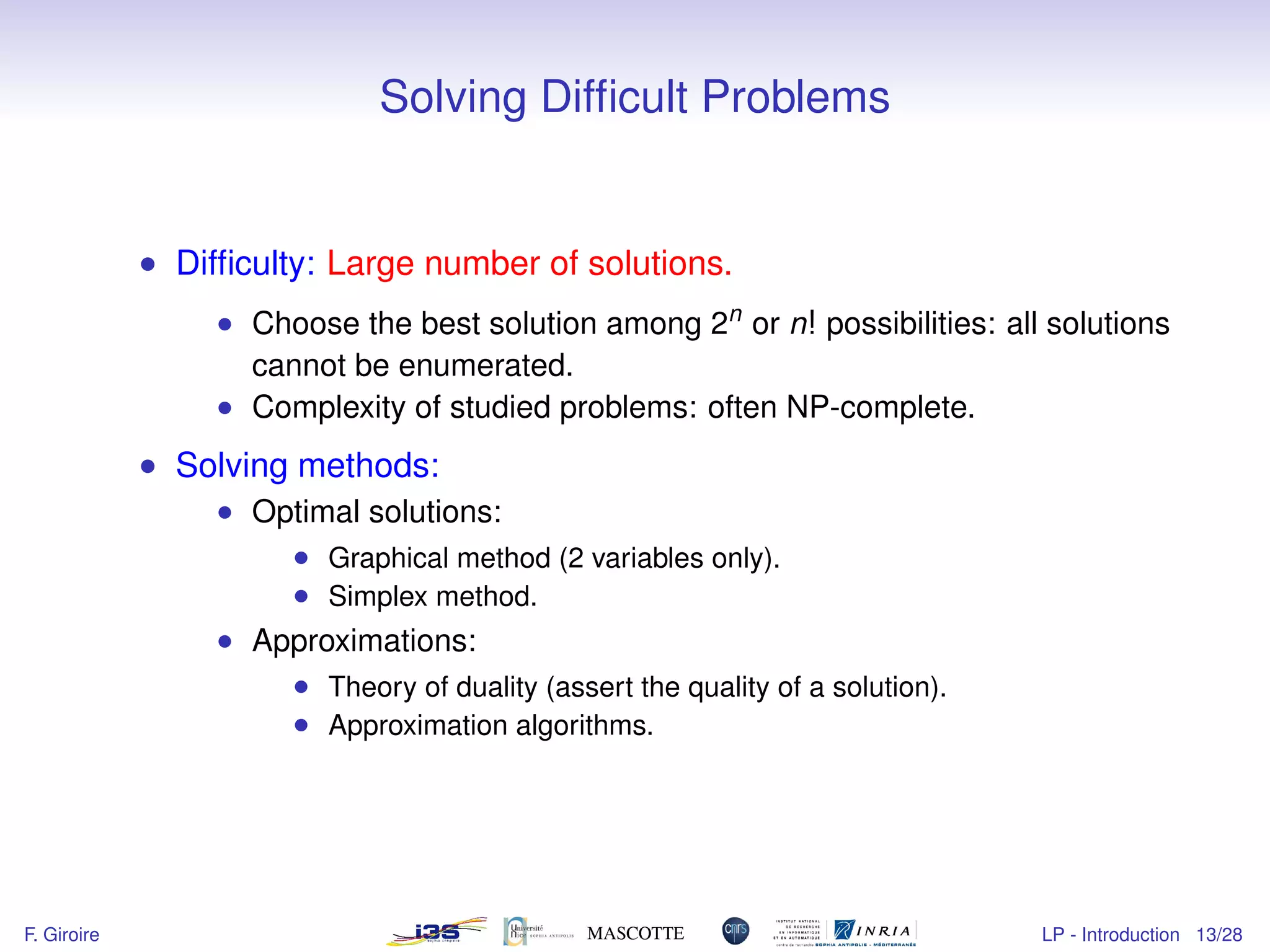
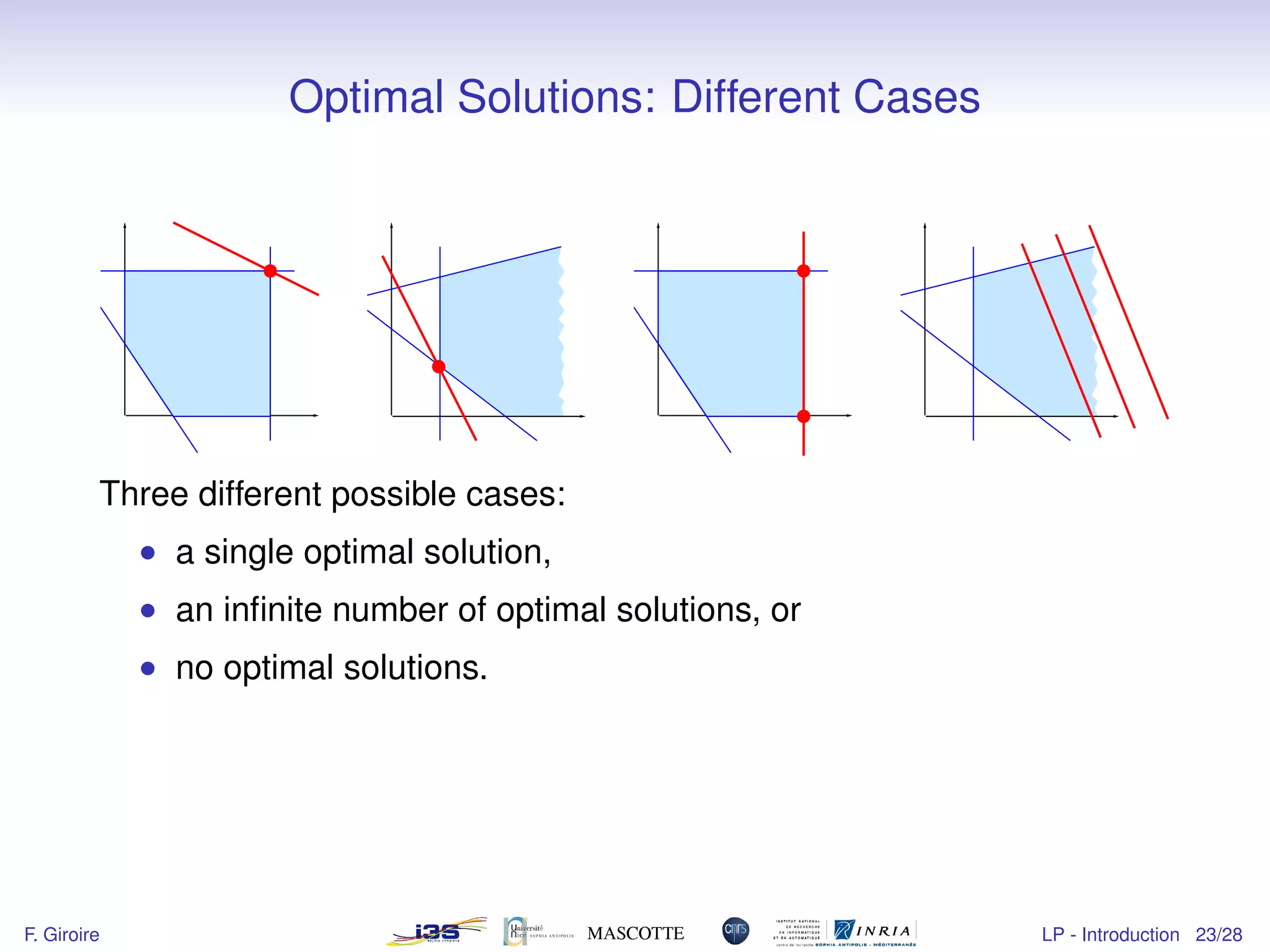
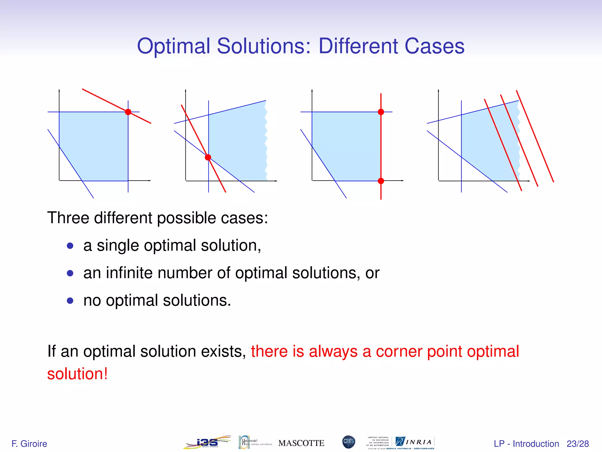
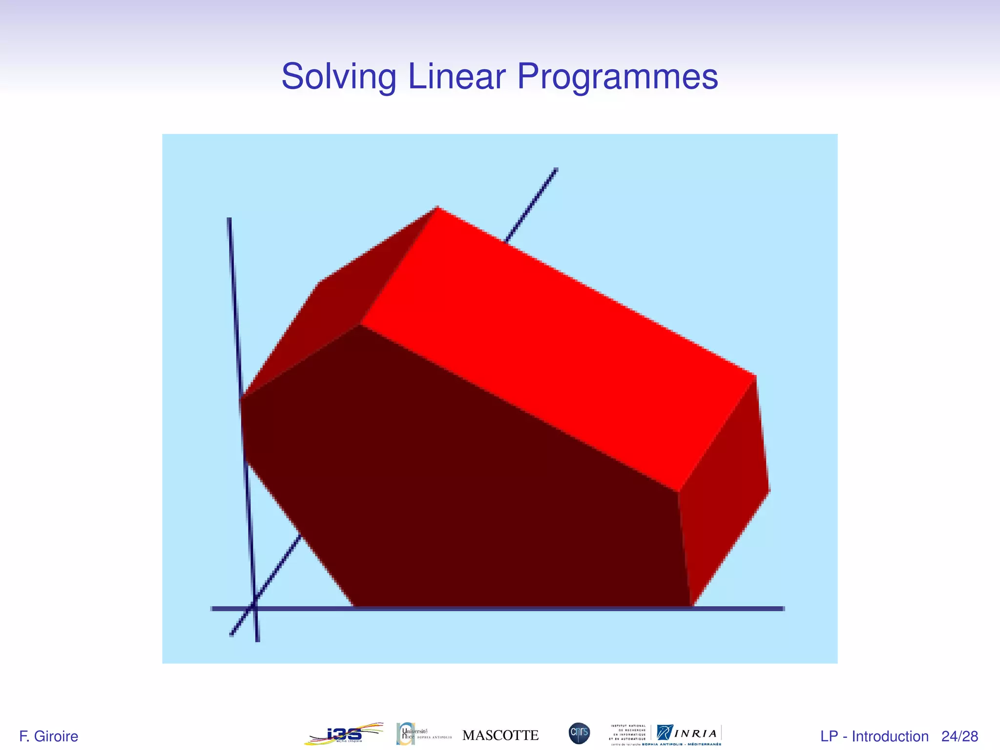
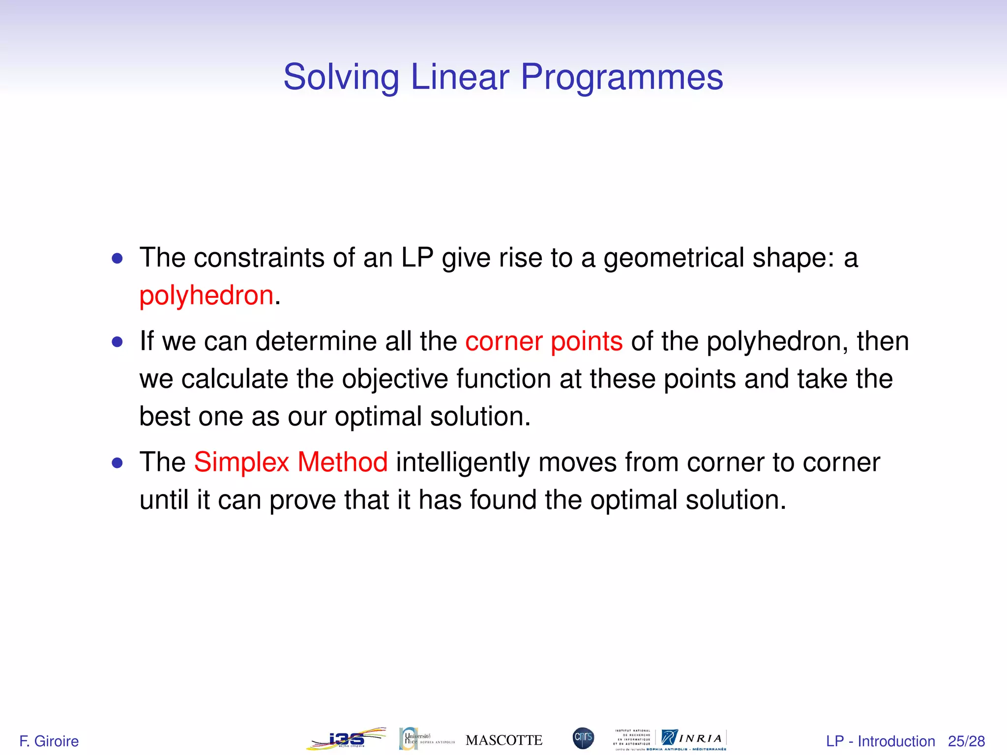
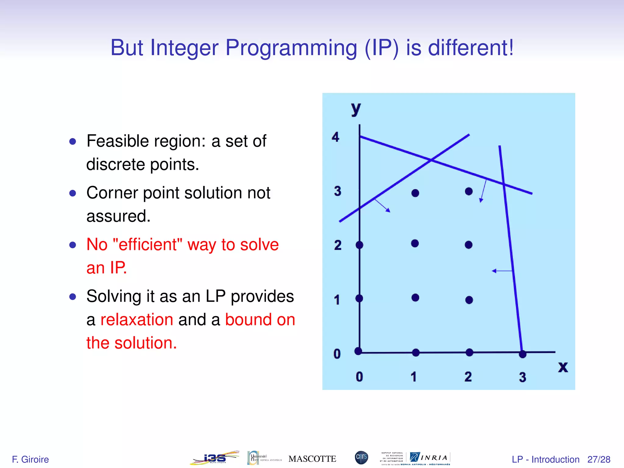
3) Linear programs can be solved efficiently using methods like the simplex algorithm, while integer programs are harder to solve optimally.