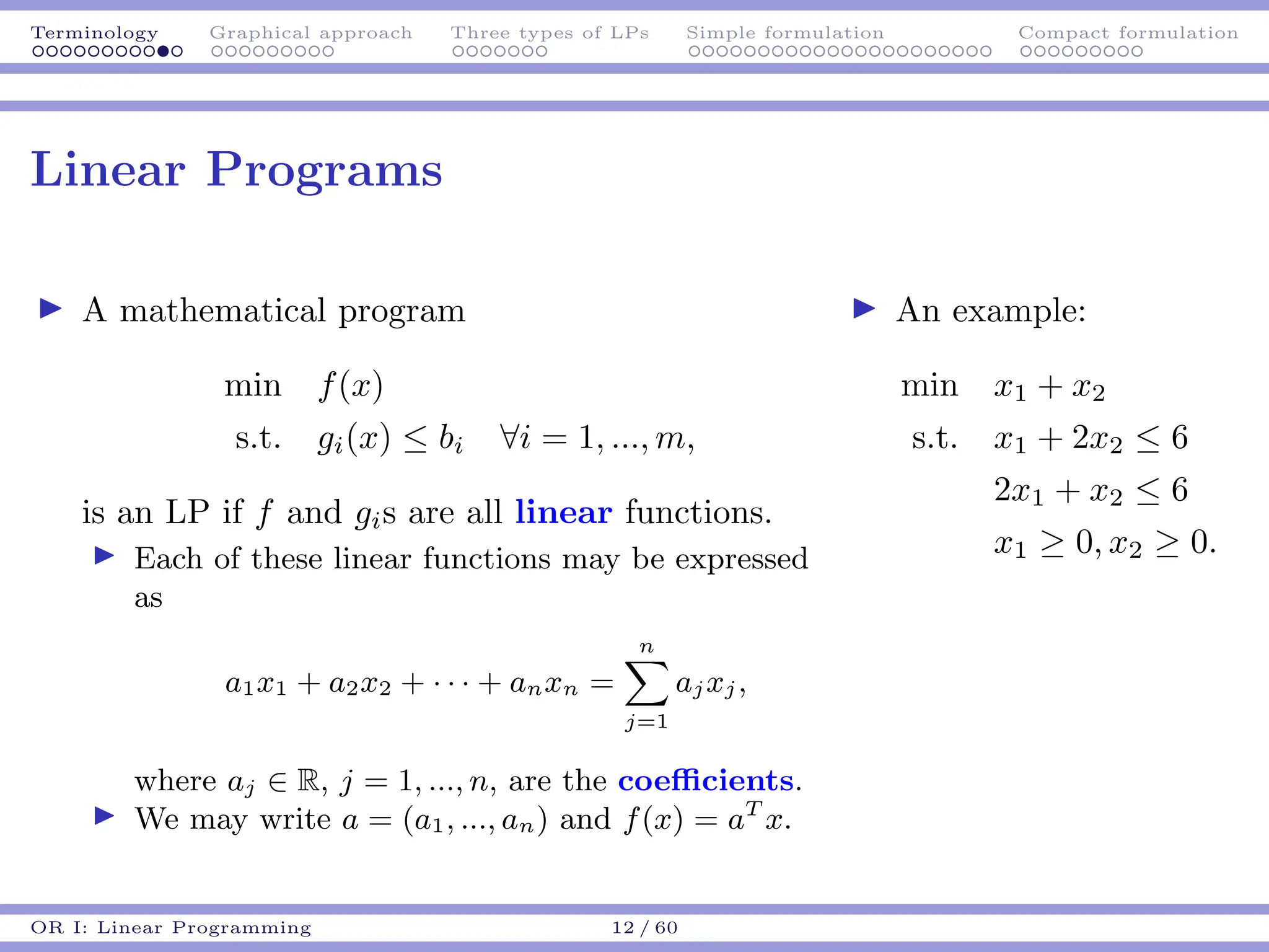
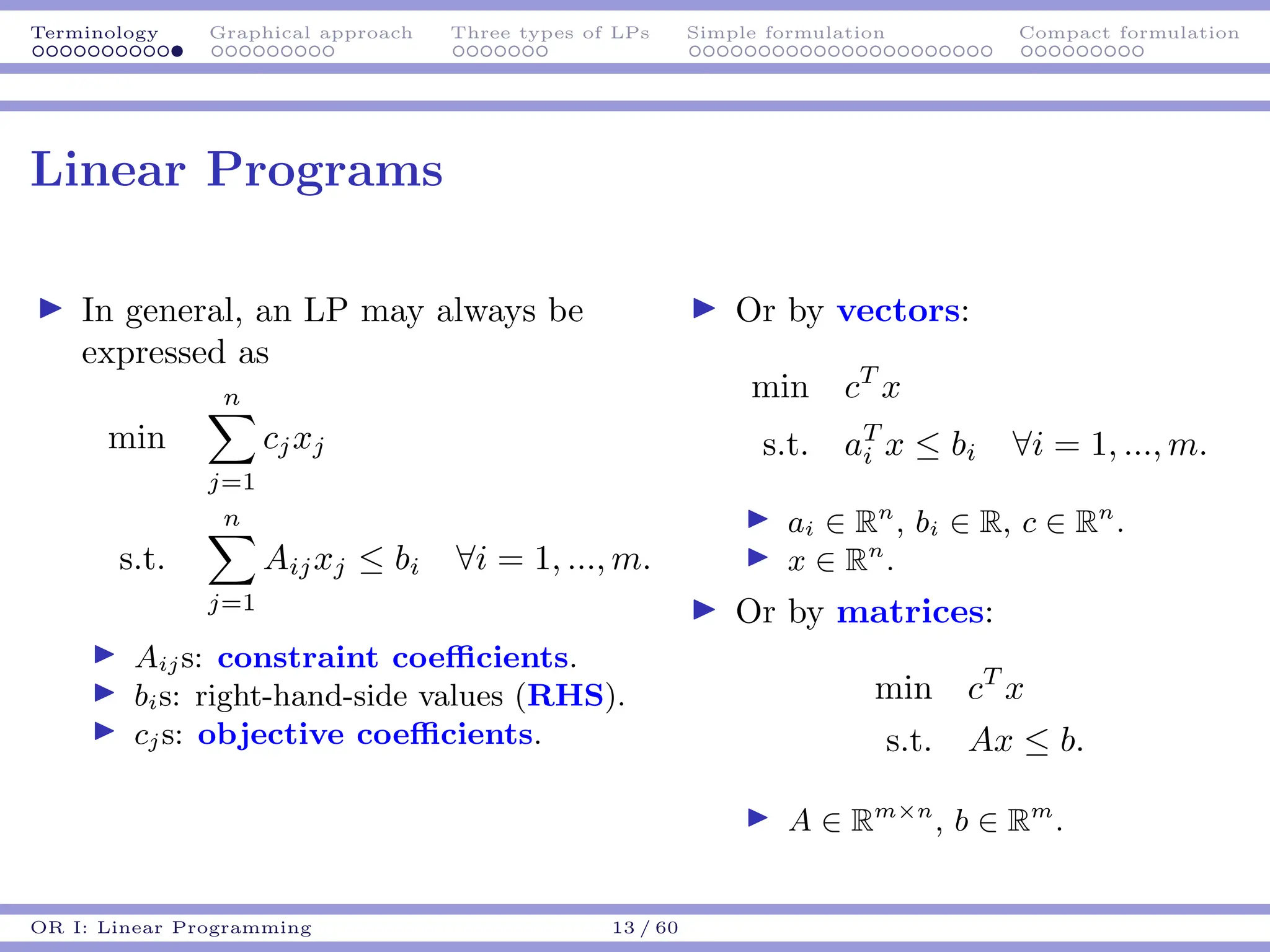
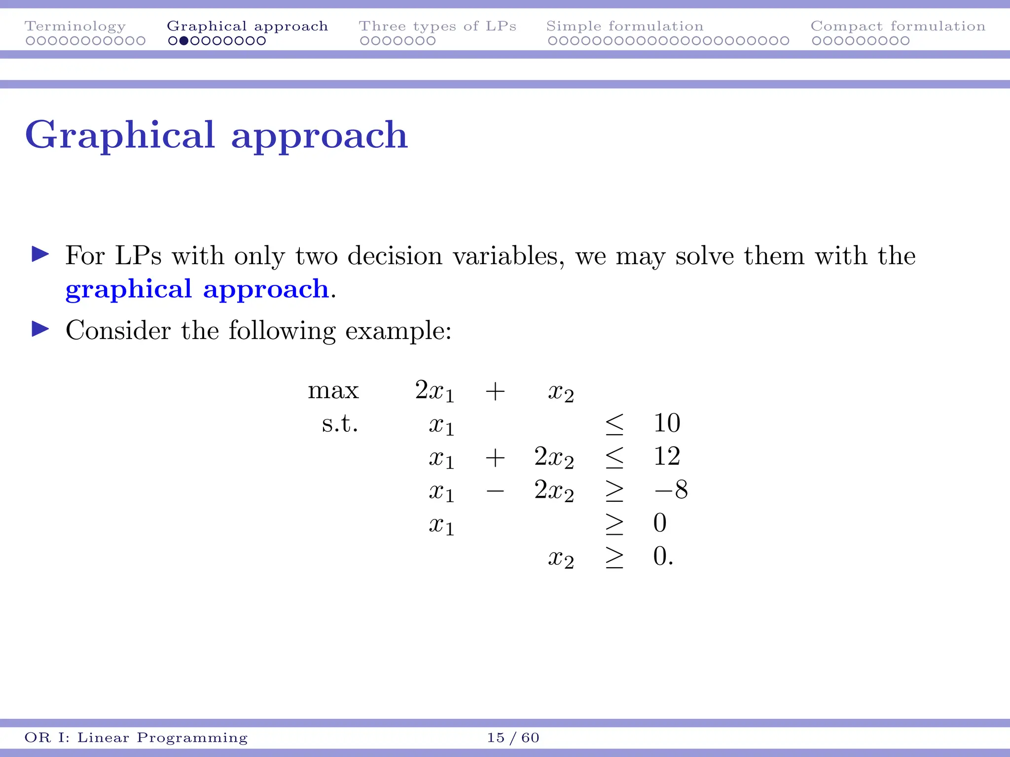
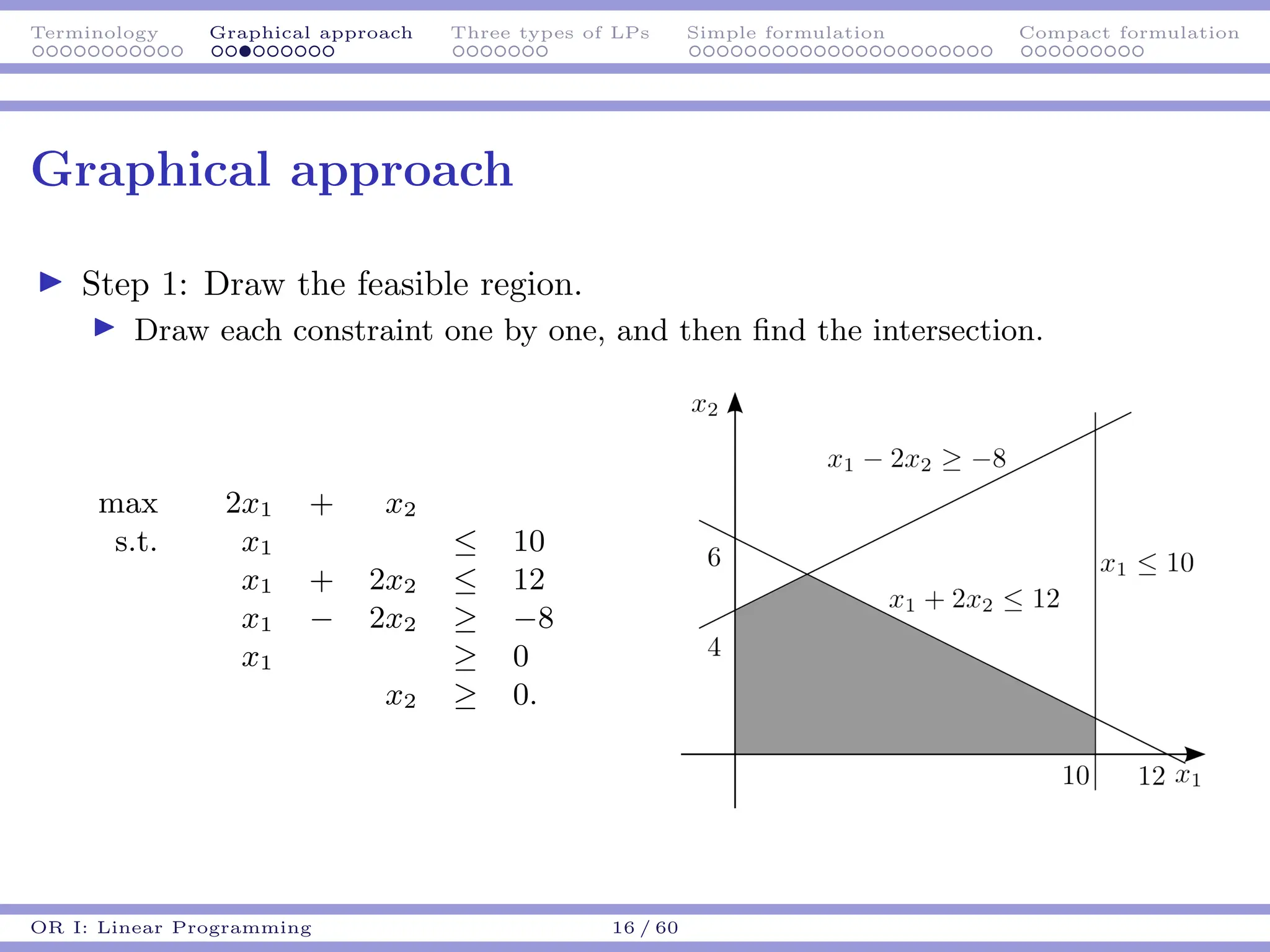
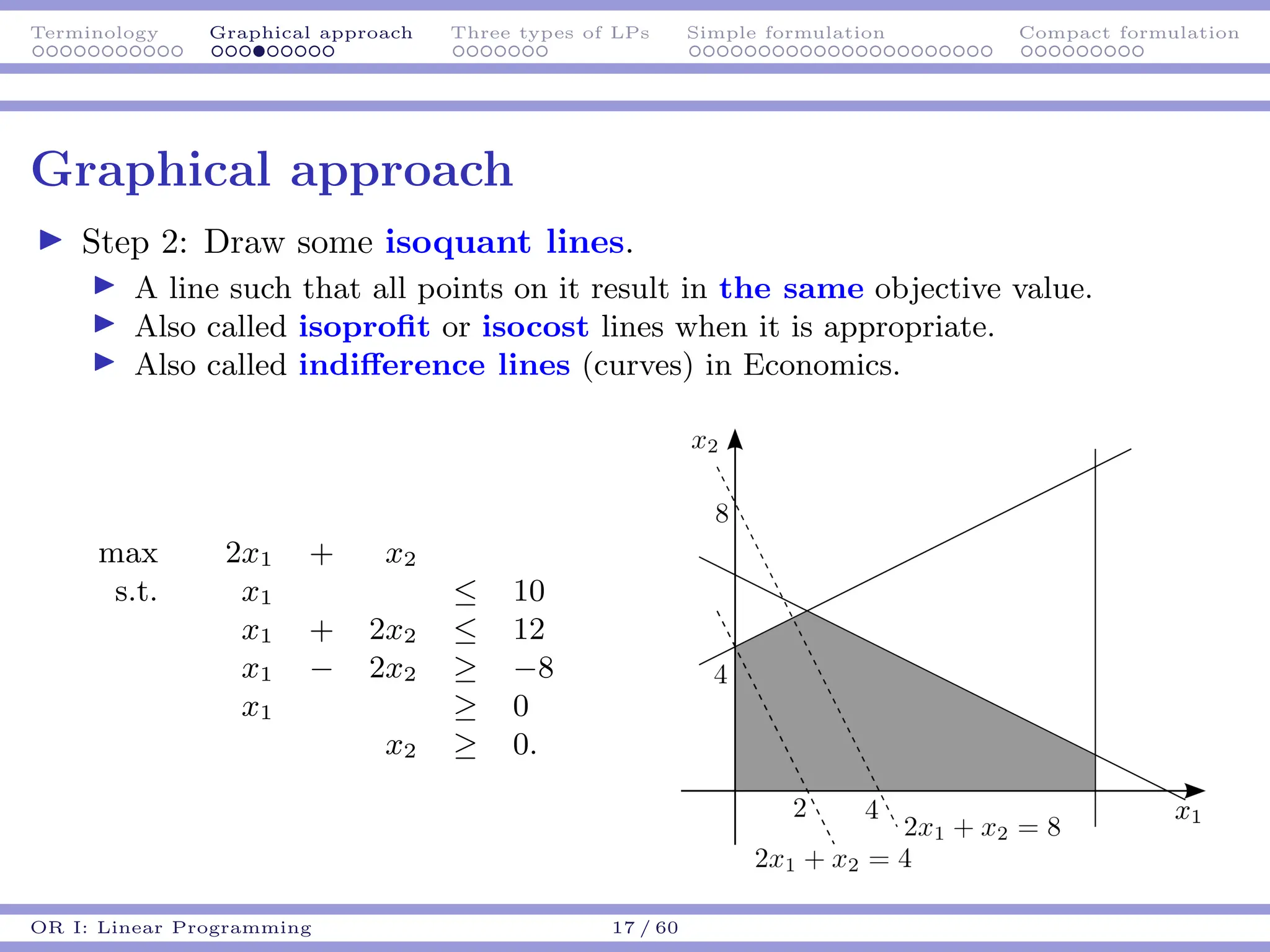
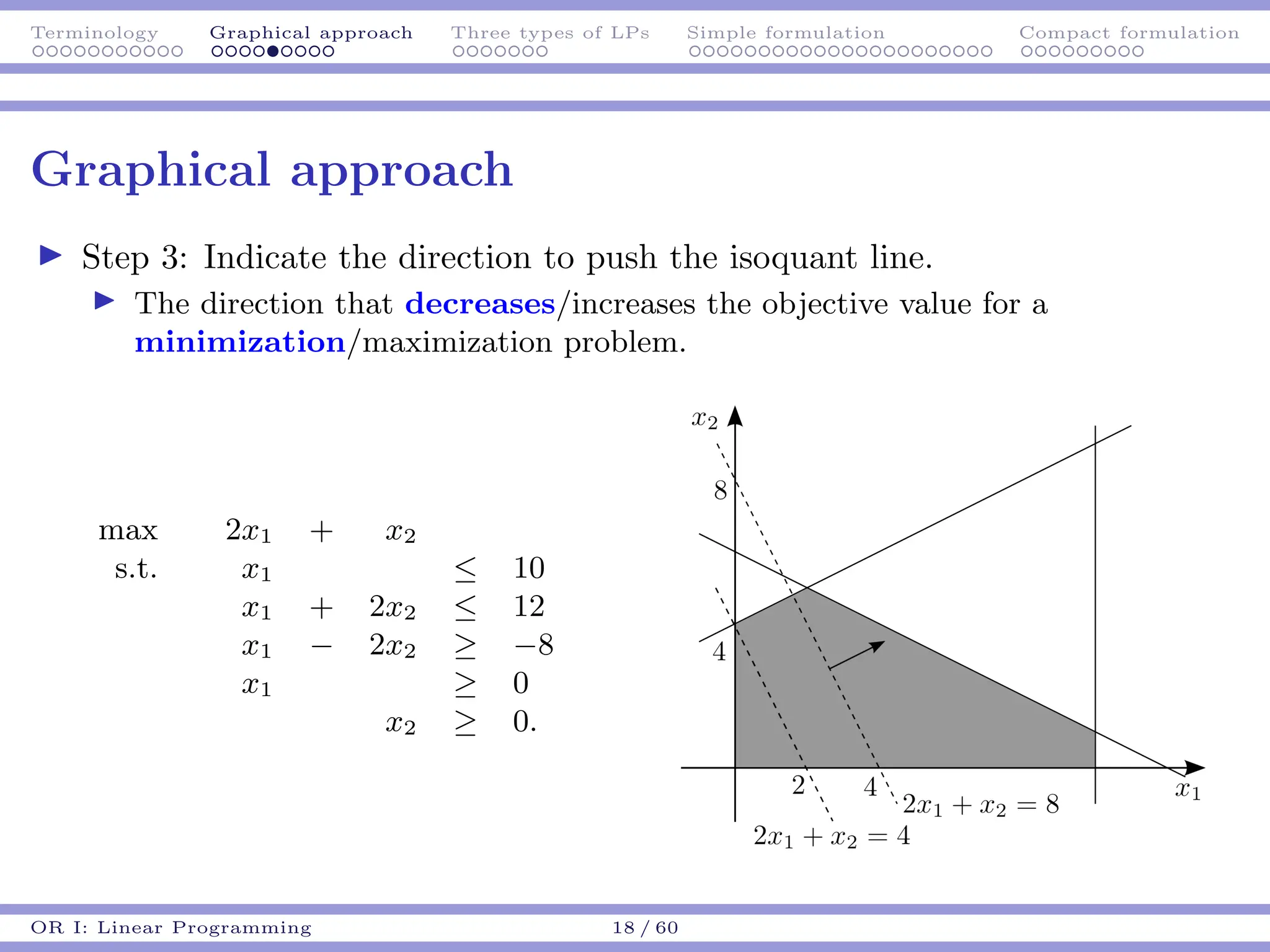
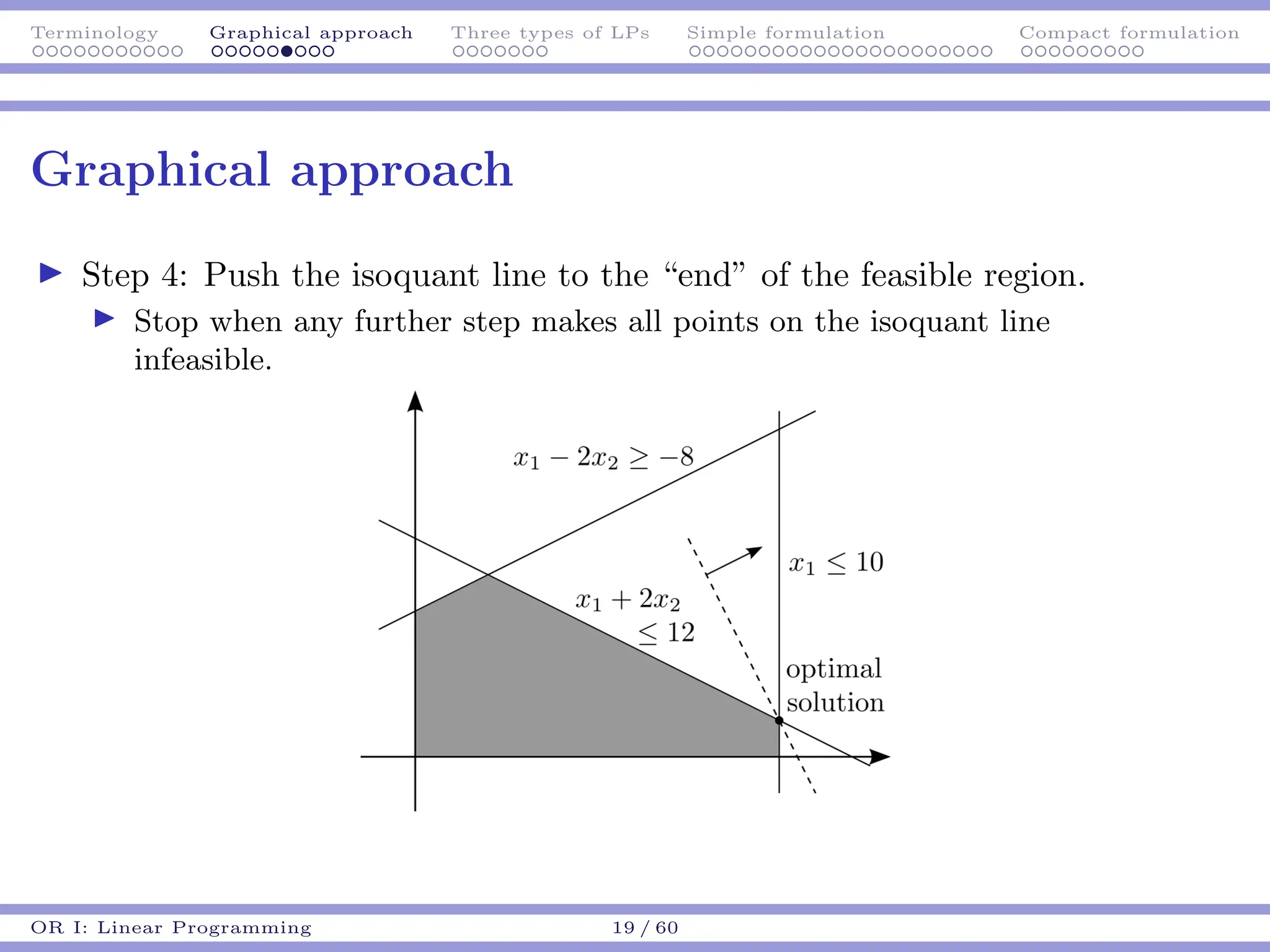
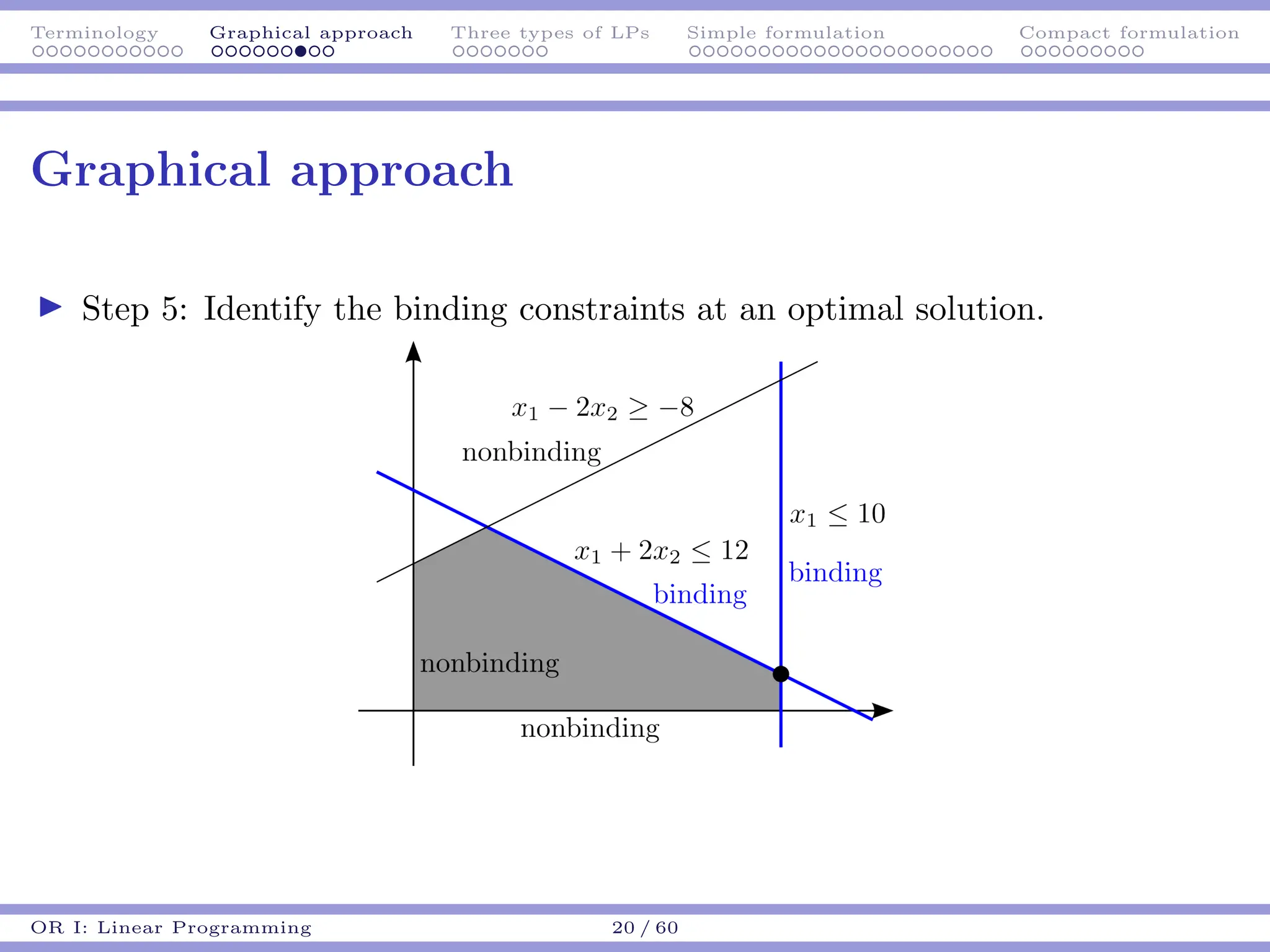
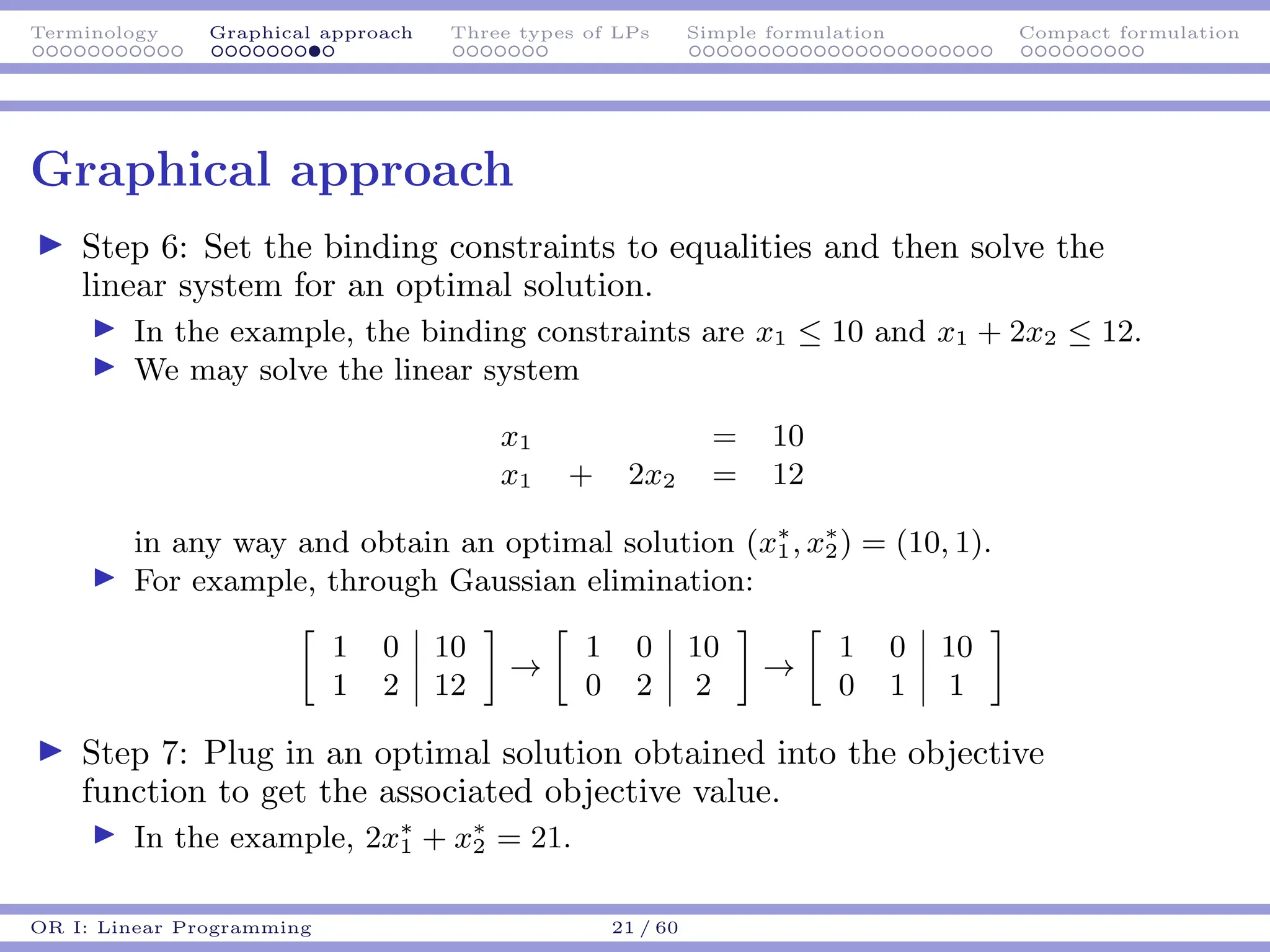
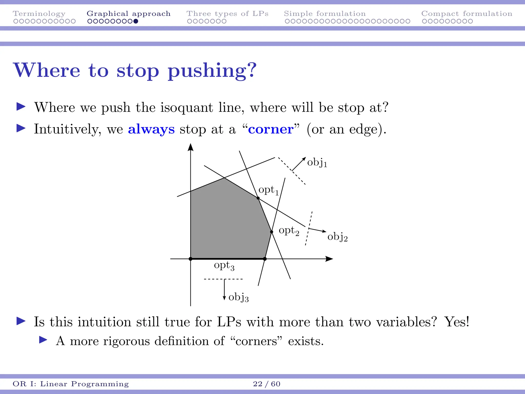
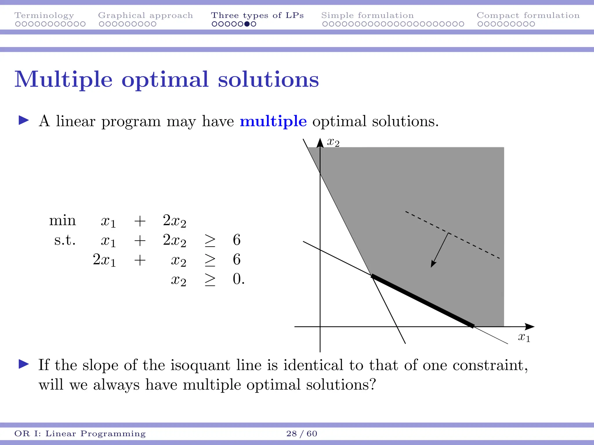
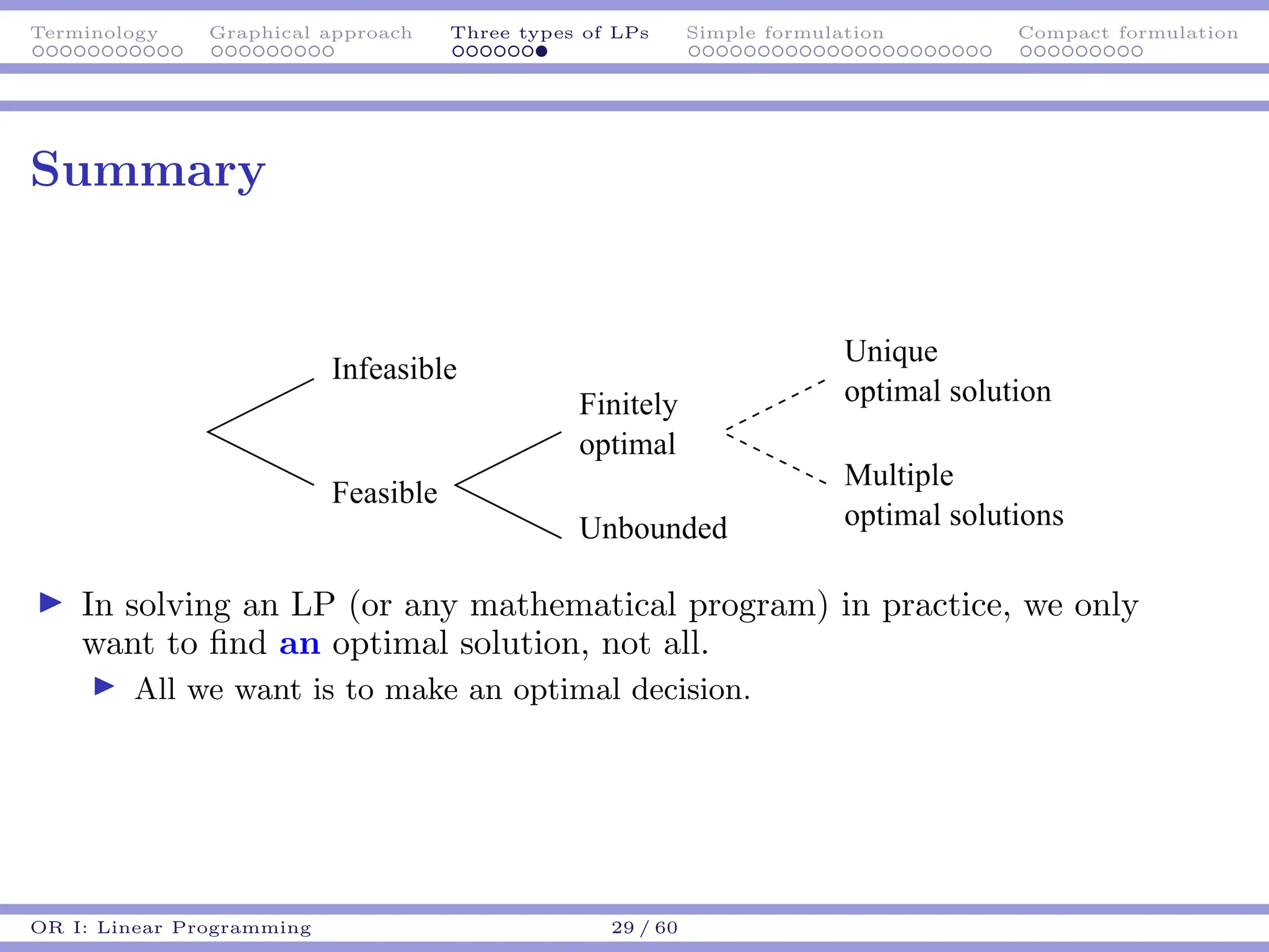
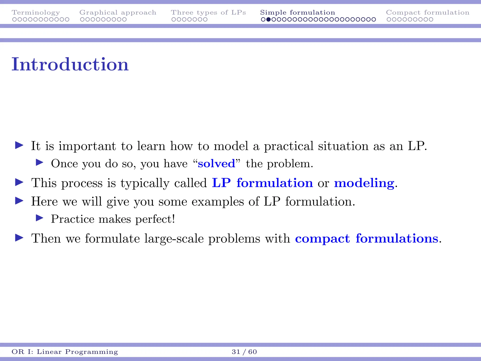
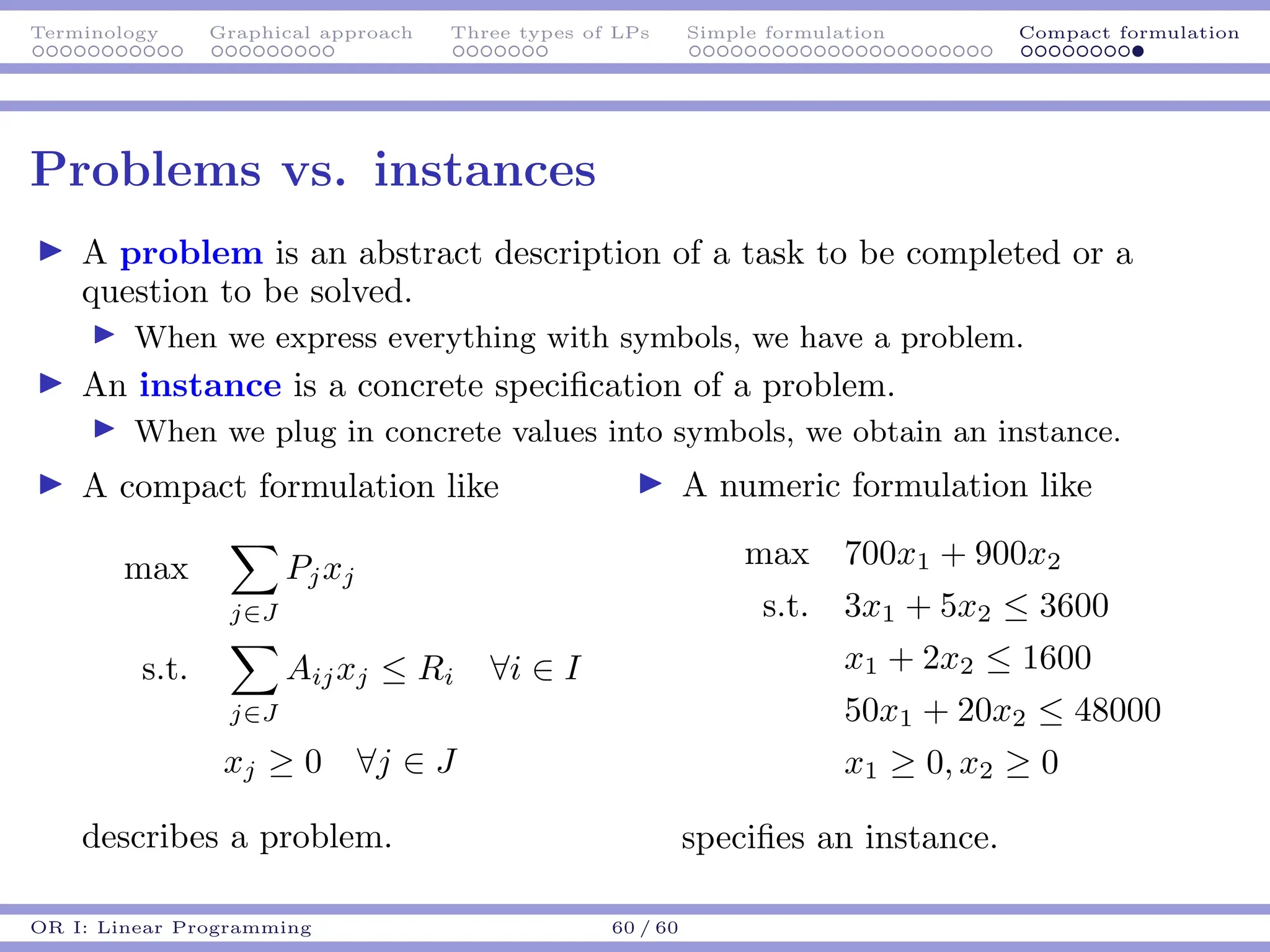
Terminology Graphical approach Three types of LPs Simple formulation Compact formulation
Operations Research I: Models & Applications
Linear Programming
Ling-Chieh Kung
Department of Information Management
National Taiwan University
OR I: Linear Programming 1 / 60
Terminology Graphical approach Three types of LPs Simple formulation Compact formulation
Introduction
▶ Let’s study Linear Programming (LP).
▶ It is used a lot in practice.
▶ It also possesses useful mathematical properties.
▶ It is a good starting point for all OR subjects.
▶ We will study:
▶ What kind of practical problems may be solved by LP.
▶ How to formulate a problem as an LP.
OR I: Linear Programming 2 / 60
Terminology Graphical approach Three types of LPs Simple formulation Compact formulation
Road map
▶ Terminology.
▶ The graphical approach.
▶ Three types of LPs.
▶ Simple LP formulations.
▶ Compact LP formulations.
OR I: Linear Programming 3 / 60
Terminology Graphical approach Three types of LPs Simple formulation Compact formulation
Linear Programs
▶ Linear Programming is the process of formulating and solving linear
programs (also abbreviated as LPs).
▶ An LP is a mathematical program with some special properties.
▶ Let’s first introduce some concepts of mathematical programs.
OR I: Linear Programming 4 / 60
Terminology Graphical approach Three types of LPs Simple formulation Compact formulation
Basic elements of a program
▶ In general, any mathematical program may be expressed as
min f(x1, x2, ..., xn) (objective function)
s.t. gi(x1, x2, ..., xn) ≤ bi ∀i = 1, ..., m (constraints)
xj ∈ R ∀j = 1, ..., n. (decision variable)
▶ There are m constraints and n variables.
▶ x1, x2, ..., and xn are real-valued decision variables.
▶ We may write
x =



x1
.
.
.
xn


 = (x1, ..., xn)
as a vector of decision variables (or a decision vector).
▶ f : Rn
→ R and gi : Rn
→ R are all real-valued functions.
▶ Mostly we will omit xj ∈ R.
OR I: Linear Programming 5 / 60
Terminology Graphical approach Three types of LPs Simple formulation Compact formulation
Transformation
▶ How about a maximization objective function?
▶ max f(x) ⇔ min −f(x).
▶ How about “=” or “≥” constraints?
▶ gi(x) ≥ bi ⇔ −gi(x) ≤ −bi.
▶ gi(x) = bi ⇔ gi(x) ≤ bi and gi(x) ≥ bi, i.e., −gi(x) ≤ −bi.
▶ For example:
max x1 − x2
s.t. −2x1 + x2 ≥ −3
x1 + 4x2 = 5.
⇔
min −x1 + x2
s.t. 2x1 − x2 ≤ 3
x1 + 4x2 ≤ 5
−x1 − 4x2 ≤ −5.
OR I: Linear Programming 6 / 60
Terminology Graphical approach Three types of LPs Simple formulation Compact formulation
Sign constraints
▶ For some reasons that will be clear in the next week, we distinguish
between two kinds of constraints:
▶ Sign constraints: xi ≥ 0 or xi ≤ 0.
▶ Functional constraints: all others.
▶ For a variable xi:
▶ It is nonnegative if xi ≥ 0.
▶ It is nonpositive if xi ≤ 0.
▶ It is unrestricted in sign (urs.) or free if it has no sign constraint.
OR I: Linear Programming 7 / 60
Terminology Graphical approach Three types of LPs Simple formulation Compact formulation
Feasible solutions
▶ For a mathematical program:
▶ A feasible solution satisfies all the constraints.
▶ An infeasible solution violates at least one constraint.
▶ For example:
min 2x1 + x2
s.t. x1 ≤ 10
x1 + 2x2 ≤ 12
x1 − 2x2 ≥ −8
x1 ≥ 0
x2 ≥ 0.
▶ Feasible?
▶ x1 = (2, 3).
▶ x2 = (6, 0).
▶ x3 = (6, 6).
OR I: Linear Programming 8 / 60
Terminology Graphical approach Three types of LPs Simple formulation Compact formulation
Feasible region and optimal solutions
▶ The feasible region (or feasible set) is the set of feasible solutions.
▶ The feasible region may be empty.
▶ An optimal solution is a feasible solution that:
▶ Attains the largest objective value for a maximization problem.
▶ Attains the smallest objective value for a minimization problem.
▶ In short, no feasible solution is better than it.
▶ An optimal solution may not be unique.
▶ There may be multiple optimal solutions.
▶ There may be no optimal solution.
OR I: Linear Programming 9 / 60
Terminology Graphical approach Three types of LPs Simple formulation Compact formulation
Binding constraints
▶ At a solution, a constraint may be binding:1
Definition 1
Let g(·) ≤ b be an inequality constraint and x̄ be a solution. g(·) ≤ b is
binding at x̄ if g(x̄) = b.
▶ An inequality is nonbinding at a point if it is strict at that point.
▶ An equality constraint is always binding at any feasible solution.
▶ Some examples:
▶ x1 + x2 ≤ 10 is binding at (x1, x2) = (2, 8).
▶ 2x1 + x2 ≥ 6 is nonbinding at (x1, x2) = (2, 8).
▶ x1 + 3x2 = 9 is binding at (x1, x2) = (6, 1).
1Binding/nonbinding constraints are also called active/inactive constraints.
OR I: Linear Programming 10 / 60
Terminology Graphical approach Three types of LPs Simple formulation Compact formulation
Strict constraints?
▶ An inequality may be strict or weak:
▶ It is strict if the two sides cannot be equal. E.g., x1 + x2 > 5.
▶ It is weak if the two sides may be equal. E.g., x1 + x2 ≥ 5.
▶ A “practical” mathematical program’s inequalities are all weak.
▶ With strict inequalities, an optimal solution may not be attainable!
▶ What is an optimal solution of
min x
s.t. x > 0?
▶ Think about budget constraints.
▶ You want to spend $500 to buy several things.
▶ Typically, you cannot spend more than $500.
▶ But you may spend exactly $500.
OR I: Linear Programming 11 / 60
Terminology Graphical approach Three types of LPs Simple formulation Compact formulation
Linear Programs
▶ A mathematical program
min f(x)
s.t. gi(x) ≤ bi ∀i = 1, ..., m,
is an LP if f and gis are all linear functions.
▶ Each of these linear functions may be expressed
as
a1x1 + a2x2 + · · · + anxn =
n
X
j=1
ajxj,
where aj ∈ R, j = 1, ..., n, are the coefficients.
▶ We may write a = (a1, ..., an) and f(x) = aT
x.
▶ An example:
min x1 + x2
s.t. x1 + 2x2 ≤ 6
2x1 + x2 ≤ 6
x1 ≥ 0, x2 ≥ 0.
OR I: Linear Programming 12 / 60
Terminology Graphical approach Three types of LPs Simple formulation Compact formulation
Linear Programs
▶ In general, an LP may always be
expressed as
min
n
X
j=1
cjxj
s.t.
n
X
j=1
Aijxj ≤ bi ∀i = 1, ..., m.
▶ Aijs: constraint coefficients.
▶ bis: right-hand-side values (RHS).
▶ cjs: objective coefficients.
▶ Or by vectors:
min cT
x
s.t. aT
i x ≤ bi ∀i = 1, ..., m.
▶ ai ∈ Rn
, bi ∈ R, c ∈ Rn
.
▶ x ∈ Rn
.
▶ Or by matrices:
min cT
x
s.t. Ax ≤ b.
▶ A ∈ Rm×n
, b ∈ Rm
.
OR I: Linear Programming 13 / 60
Terminology Graphical approach Three types of LPs Simple formulation Compact formulation
Road map
▶ Terminology.
▶ The graphical approach.
▶ Three types of LPs.
▶ Simple LP formulations.
▶ Compact LP formulations.
OR I: Linear Programming 14 / 60
Terminology Graphical approach Three types of LPs Simple formulation Compact formulation
Graphical approach
▶ For LPs with only two decision variables, we may solve them with the
graphical approach.
▶ Consider the following example:
max 2x1 + x2
s.t. x1 ≤ 10
x1 + 2x2 ≤ 12
x1 − 2x2 ≥ −8
x1 ≥ 0
x2 ≥ 0.
OR I: Linear Programming 15 / 60
Terminology Graphical approach Three types of LPs Simple formulation Compact formulation
Graphical approach
▶ Step 1: Draw the feasible region.
▶ Draw each constraint one by one, and then find the intersection.
max 2x1 + x2
s.t. x1 ≤ 10
x1 + 2x2 ≤ 12
x1 − 2x2 ≥ −8
x1 ≥ 0
x2 ≥ 0.
OR I: Linear Programming 16 / 60
Terminology Graphical approach Three types of LPs Simple formulation Compact formulation
Graphical approach
▶ Step 2: Draw some isoquant lines.
▶ A line such that all points on it result in the same objective value.
▶ Also called isoprofit or isocost lines when it is appropriate.
▶ Also called indifference lines (curves) in Economics.
max 2x1 + x2
s.t. x1 ≤ 10
x1 + 2x2 ≤ 12
x1 − 2x2 ≥ −8
x1 ≥ 0
x2 ≥ 0.
OR I: Linear Programming 17 / 60
Terminology Graphical approach Three types of LPs Simple formulation Compact formulation
Graphical approach
▶ Step 3: Indicate the direction to push the isoquant line.
▶ The direction that decreases/increases the objective value for a
minimization/maximization problem.
max 2x1 + x2
s.t. x1 ≤ 10
x1 + 2x2 ≤ 12
x1 − 2x2 ≥ −8
x1 ≥ 0
x2 ≥ 0.
OR I: Linear Programming 18 / 60
Terminology Graphical approach Three types of LPs Simple formulation Compact formulation
Graphical approach
▶ Step 4: Push the isoquant line to the “end” of the feasible region.
▶ Stop when any further step makes all points on the isoquant line
infeasible.
OR I: Linear Programming 19 / 60
Terminology Graphical approach Three types of LPs Simple formulation Compact formulation
Graphical approach
▶ Step 5: Identify the binding constraints at an optimal solution.
OR I: Linear Programming 20 / 60
Terminology Graphical approach Three types of LPs Simple formulation Compact formulation
Graphical approach
▶ Step 6: Set the binding constraints to equalities and then solve the
linear system for an optimal solution.
▶ In the example, the binding constraints are x1 ≤ 10 and x1 + 2x2 ≤ 12.
▶ We may solve the linear system
x1 = 10
x1 + 2x2 = 12
in any way and obtain an optimal solution (x∗
1, x∗
2) = (10, 1).
▶ For example, through Gaussian elimination:

1 0 10
1 2 12

→

1 0 10
0 2 2

→

1 0 10
0 1 1

▶ Step 7: Plug in an optimal solution obtained into the objective
function to get the associated objective value.
▶ In the example, 2x∗
1 + x∗
2 = 21.
OR I: Linear Programming 21 / 60
Terminology Graphical approach Three types of LPs Simple formulation Compact formulation
Where to stop pushing?
▶ Where we push the isoquant line, where will be stop at?
▶ Intuitively, we always stop at a “corner” (or an edge).
▶ Is this intuition still true for LPs with more than two variables? Yes!
▶ A more rigorous definition of “corners” exists.
OR I: Linear Programming 22 / 60
Terminology Graphical approach Three types of LPs Simple formulation Compact formulation
Road map
▶ Terminology.
▶ The graphical approach.
▶ Three types of LPs.
▶ Simple LP formulations.
▶ Compact LP formulations.
OR I: Linear Programming 23 / 60
Terminology Graphical approach Three types of LPs Simple formulation Compact formulation
Three types of LPs
▶ For any LPs, it must be one of the following:
▶ Infeasible.
▶ Unbounded.
▶ Finitely optimal (having an optimal solution).
▶ A finitely optimal LP may have:
▶ A unique optimal solution.
▶ Multiple optimal solutions.
OR I: Linear Programming 24 / 60
Terminology Graphical approach Three types of LPs Simple formulation Compact formulation
Infeasibility
▶ An LP is infeasible if its feasible region is empty.
min 3x1 + x2
s.t. x1 + x2 ≤ 4
3x1 + x2 ≥ 9
x1 − x2 ≤ 0.
OR I: Linear Programming 25 / 60
Terminology Graphical approach Three types of LPs Simple formulation Compact formulation
Unboundedness
▶ An LP is unbounded if for any feasible solution, there is another
feasible solution that is better.
max x1 + x2
s.t. x1 + 2x2 ≥ 6
2x1 + x2 ≥ 6.
OR I: Linear Programming 26 / 60
Terminology Graphical approach Three types of LPs Simple formulation Compact formulation
Unboundedness
▶ Note that an unbounded feasible region does not imply an
unbounded LP!
▶ Is it necessary?
min x1 + x2
s.t. x1 + 2x2 ≥ 6
2x1 + x2 ≥ 6.
▶ If an LP is neither infeasible nor unbounded, it is finitely optimal.
OR I: Linear Programming 27 / 60
Terminology Graphical approach Three types of LPs Simple formulation Compact formulation
Multiple optimal solutions
▶ A linear program may have multiple optimal solutions.
min x1 + 2x2
s.t. x1 + 2x2 ≥ 6
2x1 + x2 ≥ 6
x2 ≥ 0.
▶ If the slope of the isoquant line is identical to that of one constraint,
will we always have multiple optimal solutions?
OR I: Linear Programming 28 / 60
Terminology Graphical approach Three types of LPs Simple formulation Compact formulation
Summary
▶ In solving an LP (or any mathematical program) in practice, we only
want to find an optimal solution, not all.
▶ All we want is to make an optimal decision.
OR I: Linear Programming 29 / 60
Terminology Graphical approach Three types of LPs Simple formulation Compact formulation
Road map
▶ Terminology.
▶ The graphical approach.
▶ Three types of LPs.
▶ Simple LP formulations.
▶ Compact LP formulations.
OR I: Linear Programming 30 / 60
Terminology Graphical approach Three types of LPs Simple formulation Compact formulation
Introduction
▶ It is important to learn how to model a practical situation as an LP.
▶ Once you do so, you have “solved” the problem.
▶ This process is typically called LP formulation or modeling.
▶ Here we will give you some examples of LP formulation.
▶ Practice makes perfect!
▶ Then we formulate large-scale problems with compact formulations.
OR I: Linear Programming 31 / 60
Terminology Graphical approach Three types of LPs Simple formulation Compact formulation
A product mix problem
▶ We produce several products to sell.
▶ Each product requires some resources. Resources are limited.
▶ We want to maximize the total sales revenue with available resources.
OR I: Linear Programming 32 / 60
Terminology Graphical approach Three types of LPs Simple formulation Compact formulation
Problem description
▶ We produce desks and tables.
▶ Producing a desk requires three units of wood, one hour of labor, and 50
minutes of machine time.
▶ Producing a table requires five units of wood, two hours of labor, and 20
minutes of machine time.
▶ We may sell everything we produce.
▶ For each day, we have
▶ Two hundred workers that each works for eight hours.
▶ Fifty machines that each runs for sixteen hours.
▶ A supply of 3600 units of wood.
▶ Desks and tables are sold at $700 and $900 per unit, respectively.
OR I: Linear Programming 33 / 60
Terminology Graphical approach Three types of LPs Simple formulation Compact formulation
Define variables
▶ What do we need to decide?
▶ Let
x1 = number of desks produced in a day and
x2 = number of tables produced in a day.
▶ With these variables, we now try to express how much we will earn
and how many resources we will consume.
OR I: Linear Programming 34 / 60
Terminology Graphical approach Three types of LPs Simple formulation Compact formulation
Formulate the objective function
▶ We want to maximize the total sales revenue.
▶ Given our variables x1 and x2, the sales revenue is 700x1 + 900x2.
▶ The objective function is thus
max 700x1 + 900x2.
OR I: Linear Programming 35 / 60
Terminology Graphical approach Three types of LPs Simple formulation Compact formulation
Formulate constraints
▶ For each restriction or limitation, we write a constraint:
Resource
Consumption per
Total supply
Desk Table
Wood 3 units 5 units 3600 units
Labor
1 hour 2 hours
200 workers × 8 hr/worker
hour = 1600 hours
Machine
50 minutes 20 minutes
50 machines × 16 hr/machine
time = 800 hours
▶ The supply of wood is limited: 3x1 + 5x2 ≤ 3600.
▶ The number of labor hours is limited: x1 + 2x2 ≤ 1600.
▶ The amount of machine time is limited: 50x1 + 20x2 ≤ 48000.
▶ Use the same unit of measurement!
OR I: Linear Programming 36 / 60
Terminology Graphical approach Three types of LPs Simple formulation Compact formulation
Complete formulation
▶ Collectively, our formulation is
max
s.t.
700x1 + 900x2
3x1 + 5x2 ≤ 3600 (wood)
x1 + 2x2 ≤ 1600 (labor)
50x1 + 20x2 ≤ 48000 (machine)
x1 ≥ 0
x2 ≥ 0.
▶ In any case:
▶ Clearly define decision variables in front of your formulation.
▶ Write comments after the objective function and constraints.
OR I: Linear Programming 37 / 60
Terminology Graphical approach Three types of LPs Simple formulation Compact formulation
Solve and interpret
▶ An optimal solution of this LP is (884.21, 189.47).
▶ So the interpretation is... to produce 884.21 desks and 189.47 tables?
▶ “Producing 884.21 desks and 189.47 tables” seems weird, but in fact:
▶ We may produce 884.21 desks and 189.47 tables per day in average
(i.e., roughly 88,420 desks and 18,947 tables per 100 days).
▶ We may suggest to produce, e.g., 884 desks and 189 tables.2
▶ It still supports our decision making.
▶ It may not really be optimal, but we spend a very short time to make a
good suggestion.
▶ “All models are wrong, but some are useful.”
2Why not 885 desks and 190 tables or the other two ways of rounding?
OR I: Linear Programming 38 / 60
Terminology Graphical approach Three types of LPs Simple formulation Compact formulation
Produce and store!
▶ When we are making decisions, we may also consider what will happen
in the future.
▶ This creates multi-period problems.
▶ In many cases, products produced today may be stored and then sold
in the future.
▶ Maybe daily capacity is not enough.
▶ Maybe production is cheaper today.
▶ Maybe the price is higher in the future.
▶ So the production decision must be jointly considered with the
inventory decision.
OR I: Linear Programming 39 / 60
Terminology Graphical approach Three types of LPs Simple formulation Compact formulation
Problem description
▶ We produce and sell a product.
▶ For the coming four days, the marketing manager has promised to
fulfill the following amount of demands:
▶ Days 1, 2, 3, and 4: 100, 150, 200, and 170 units, respectively.
▶ The unit production costs are different for different days:
▶ Days 1, 2, 3, and 4: $9, $12, $10, and $12 per unit, respectively.
▶ The prices are all fixed. So maximizing profits is the same as
minimizing costs.
▶ We may store a product and sell it later.
▶ The inventory cost is $1 per unit per day.3
▶ E.g., producing 620 units on day 1 to fulfill all demands costs
$9 × 620 + $1 × 150 + $2 × 200 + $3 × 170 = $6, 640.
3Where does this inventory cost come from?
OR I: Linear Programming 40 / 60
Terminology Graphical approach Three types of LPs Simple formulation Compact formulation
Problem description: timing
▶ Timing:
▶ Beginning inventory + production − sales = ending inventory.
▶ Inventory costs are calculated according to ending inventory.
OR I: Linear Programming 41 / 60
Terminology Graphical approach Three types of LPs Simple formulation Compact formulation
Variables and objective function
▶ Let
xt = production quantity of day t, t = 1, ..., 4.
yt = ending inventory of day t, t = 1, ..., 4.
▶ It is important to specify “ending”!
▶ The objective function is
min 9x1 + 12x2 + 10x3 + 12x4 + y1 + y2 + y3 + y4.
OR I: Linear Programming 42 / 60
Terminology Graphical approach Three types of LPs Simple formulation Compact formulation
Constraints
▶ We need to keep an eye on our inventory:
▶ Day 1: x1 − 100 = y1.
▶ Day 2: y1 + x2 − 150 = y2.
▶ Day 3: y2 + x3 − 200 = y3.
▶ Day 4: y3 + x4 − 170 = y4.
▶ These are typically called inventory balancing constraints.
▶ We also need to fulfill all demands at the moment of sales:
▶ x1 ≥ 100, y1 + x2 ≥ 150, y2 + x3 ≥ 200, and y3 + x4 ≥ 170.
▶ Also, production and inventory quantities cannot be negative.
OR I: Linear Programming 43 / 60
Terminology Graphical approach Three types of LPs Simple formulation Compact formulation
The complete formulation
▶ The complete formulation is
min 9x1 + 12x2 + 10x3 + 12x4 + y1 + y2 + y3 + y4
s.t. x1 − 100 = y1
y1 + x2 − 150 = y2
y2 + x3 − 200 = y3
y3 + x4 − 170 = y4
x1 ≥ 100
y1 + x2 ≥ 150
y2 + x3 ≥ 200
y3 + x4 ≥ 170
xt, yt ≥ 0 ∀t = 1, ..., 4.
OR I: Linear Programming 44 / 60
Terminology Graphical approach Three types of LPs Simple formulation Compact formulation
Simplifying the formulation
▶ May we simplify the formulation?
▶ Inventory balancing and nonnegativity imply demand fulfillment!
▶ E.g., in day 1, x1 − 100 = y1 and y1 ≥ 0 means x1 ≥ 100.
▶ So the formulation may be simplified to
min 9x1 + 12x2 + 10x3 + 12x4 + y1 + y2 + y3 + y4
s.t. x1 − 100 = y1
y1 + x2 − 150 = y2
y2 + x3 − 200 = y3
y3 + x4 − 170 = y4
xt ≥ 0, yt ≥ 0 ∀t = 1, ..., 4.
▶ Identifying redundant constraints (removing them does not alter the
feasible region) helps reduce the complexity of a program.
OR I: Linear Programming 45 / 60
Terminology Graphical approach Three types of LPs Simple formulation Compact formulation
Simplifying the formulation
▶ One may further argue that there is no need to have ending inventory
in period 4 (because it is costly but useless).
▶ So the formulation may be further simplified to
min 9x1 + 12x2 + 10x3 + 12x4 + y1 + y2 + y3
s.t. x1 − 100 = y1, y1 + x2 − 150 = y2
y2 + x3 − 200 = y3, y3 + x4 − 170 = 0
xt ≥ 0 ∀t = 1, ..., 4
yt ≥ 0 ∀t = 1, ..., 3.
▶ However, this is not always suggested (at this stage).
▶ It is not required because a solver will see this.
▶ It is too difficult if the instance scale is large.
▶ In summary, simplification is good but in most cases unnecessary.
OR I: Linear Programming 46 / 60
Terminology Graphical approach Three types of LPs Simple formulation Compact formulation
Personnel scheduling
▶ We are scheduling employees in a department store.
▶ Each employee must work for five consecutive days and then take
rests for two consecutive days.
▶ The number of employees required for each day:
Mon Tue Wed Thu Fri Sat Sun
110 80 150 30 70 160 120
▶ There are seven shifts: Monday to Friday, Tuesday to Saturday, ...,
and Sunday to Thursday.
▶ We want to minimize the number of employees hired.
OR I: Linear Programming 47 / 60
Terminology Graphical approach Three types of LPs Simple formulation Compact formulation
Personnel scheduling
▶ We may find a feasible solution easily.
▶ For example, we may assign 150 employees to work from Monday to
Friday and 160 to work from Saturday to Wednesday:
Mon Tue Wed Thu Fri Sat Sun
Demand 110 80 150 30 70 160 120
Shift 1 150 150 150 150 150
Shift 6 160 160 160 160 160
Total 310 310 310 150 150 160 160
▶ This solution is feasible but seems to be bad.
OR I: Linear Programming 48 / 60
Terminology Graphical approach Three types of LPs Simple formulation Compact formulation
Decision variables and objective function
▶ Let Monday be day 1, Tuesday be day 2, etc.
▶ Let xi be the number of employees who starts to work from day i for
five consecutive days.
▶ xi is the number of employees assigned to shift i.
▶ The objective function is thus:
min x1 + x2 + x3 + x4 + x5 + x6 + x7.
OR I: Linear Programming 49 / 60
Terminology Graphical approach Three types of LPs Simple formulation Compact formulation
Constraints
▶ Demand fulfillment:
▶ 110 employees are needed on Monday:
x1 + x4 + x5 + x6 + x7 ≥ 110.
▶ 80 employees are needed on Tuesday:
x1 + x2 + x5 + x6 + x7 ≥ 80.
▶ 120 employees are needed on Sunday:
x3 + x4 + x5 + x6 + x7 ≥ 120.
▶ Nonnegativity constraints:
xi ≥ 0 ∀i = 1, ..., 7.
OR I: Linear Programming 50 / 60
Terminology Graphical approach Three types of LPs Simple formulation Compact formulation
Complete formulation
▶ The complete formulation is
min x1 + x2 + x3 + x4 + x5 + x6 + x7
s.t. x1 + x4 + x5 + x6 + x7 ≥ 110
x1 + x2 + x5 + x6 + x7 ≥ 80
x1 + x2 + x3 + x6 + x7 ≥ 150
x1 + x2 + x3 + x4 + x7 ≥ 30
x1 + x2 + x3 + x4 + x5 ≥ 70
x2 + x3 + x4 + x5 + x6 ≥ 160
x3 + x4 + x5 + x6 + x7 ≥ 120
xi ≥ 0 ∀i = 1, ..., 7.
OR I: Linear Programming 51 / 60
Terminology Graphical approach Three types of LPs Simple formulation Compact formulation
Road map
▶ Terminology.
▶ The graphical approach.
▶ Three types of LPs.
▶ Simple LP formulations.
▶ Compact LP formulations.
OR I: Linear Programming 52 / 60
Terminology Graphical approach Three types of LPs Simple formulation Compact formulation
Compact formulations
▶ Most problem instances in practice are of large scales.
▶ The number of variables and constraints are huge.
▶ Many variables may be grouped together:
▶ E.g., xt = production quantity of day t, t = 1, ..., 4.
▶ Many constraints may be grouped together:
▶ E.g., xt ≥ 0 for all t = 1, ..., 4.
▶ In modeling large-scale instances, we use compact formulations to
enhance readability and efficiency.
▶ We use the following three instruments:
▶ Indices (i, j, k, ...).
▶ Summation (
P
).
▶ For all (∀).
OR I: Linear Programming 53 / 60
Terminology Graphical approach Three types of LPs Simple formulation Compact formulation
Compact objective function
▶ The production-inventory problem:
▶ We have several periods. In each period, we first produce and then sell.
▶ Unsold products become ending inventories.
▶ We want to minimize the total cost.
▶ Indices: Because things will repeat in each period, it is natural to
use an index for periods. Let t ∈ {1, ..., 4} be the index of periods.
▶ For the objective function:
min 9x1 + 12x2 + 10x3 + 12x4 + y1 + y2 + y3 + y4,
if we denote the unit production cost on day t as Ct, t = 1, ..., 4, we
may rewrite it as
min
4
X
t=1
(Ctxt + yt).
OR I: Linear Programming 54 / 60
Terminology Graphical approach Three types of LPs Simple formulation Compact formulation
Compacting the constraints
▶ The original constraints:
▶ x1 − 100 = y1, y1 + x2 − 150 = y2, y2 + x3 − 200 = y3, y3 + x4 − 170 = y4.
▶ Let’s denote the demand on day t as Dt, t = 1, ..., 4:
▶ For t = 2, ..., 4 : yt−1 + xt − Dt = yt.
▶ We cannot apply this to day 1 as y0 is undefined!
▶ To group the four constraints into one compact constraint, we add an
additional decision variable y0:
yt = ending inventory of day t, t = 0, ..., 4.
▶ Then the set of inventory balancing constraints are written as
yt−1 + xt − Dt = yt ∀t = 1, ..., 4.
▶ Certainly we need to set up the initial inventory: y0 = 0.
OR I: Linear Programming 55 / 60
Terminology Graphical approach Three types of LPs Simple formulation Compact formulation
The complete compact formulation
▶ The compact formulation is
min
4
X
t=1
(Ctxt + yt)
s.t. yt−1 + xt − Dt = yt ∀t = 1, ..., 4
y0 = 0
xt, yt ≥ 0 ∀t = 1, ..., 4.
▶ Do not forget those for-all statements! Without them, the formulation
is wrong.
▶ Nonnegativity constraints for multiple sets of variables may be combined
to save some “≥ 0”.
▶ One convention is to:
▶ Use lowercase letters for variables (e.g., xt).
▶ Use uppercase letters for parameters (e.g., Ct).
OR I: Linear Programming 56 / 60
Terminology Graphical approach Three types of LPs Simple formulation Compact formulation
Parameter declaration
▶ When creating parameter sets, we write something like
denote Ct as the unit production cost on day t, t = 1, ..., 4.
▶ Do not need to specify values, even though we have those values.
▶ Need to specify the range through indices.
▶ Parameter declarations should be at the beginning of the formulation.
▶ Parameters and variables are different.
▶ Variables are those to be determined. We do not know their values
before we solve the model.
▶ Parameters are given with known values.
▶ Parameters are exogenous and variables are endogenous.
OR I: Linear Programming 57 / 60
Terminology Graphical approach Three types of LPs Simple formulation Compact formulation
Compact formulation for product mix
▶ Consider the product mix problem.
▶ Let n be the number of products and m be the number of resources.
▶ Let j and i be the indices for products and resources, respectively.
▶ We denote the unit sales price of product j as Pj, supply limit of
resources i as Ri, and unit of resource i required for producing one unit
of product j as Aij, where i = 1, ..., m, j = 1, ..., n.
▶ Let xj be the production quantity for product j, j = 1, ..., n.
▶ The compact formulation is
max
n
X
j=1
Pjxj
s.t.
n
X
j=1
Aijxj ≤ Ri ∀i = 1, ..., m
xj ≥ 0 ∀j = 1, ..., n.
OR I: Linear Programming 58 / 60
Terminology Graphical approach Three types of LPs Simple formulation Compact formulation
Compact formulation for product mix
▶ Alternatively, let’s define J = {1, ..., n} as the set of products and
I = {1, ..., m} be the set of resources.
▶ The compact formulation is
max
X
j∈J
Pjxj
s.t.
X
j∈J
Aijxj ≤ Ri ∀i ∈ I
xj ≥ 0 ∀j ∈ J.
OR I: Linear Programming 59 / 60
Terminology Graphical approach Three types of LPs Simple formulation Compact formulation
Problems vs. instances
▶ A problem is an abstract description of a task to be completed or a
question to be solved.
▶ When we express everything with symbols, we have a problem.
▶ An instance is a concrete specification of a problem.
▶ When we plug in concrete values into symbols, we obtain an instance.
▶ A compact formulation like
max
X
j∈J
Pjxj
s.t.
X
j∈J
Aijxj ≤ Ri ∀i ∈ I
xj ≥ 0 ∀j ∈ J
describes a problem.
▶ A numeric formulation like
max 700x1 + 900x2
s.t. 3x1 + 5x2 ≤ 3600
x1 + 2x2 ≤ 1600
50x1 + 20x2 ≤ 48000
x1 ≥ 0, x2 ≥ 0
specifies an instance.
OR I: Linear Programming 60 / 60

Linear programming problems and models.pdf

  • 1.
    Terminology Graphical approachThree types of LPs Simple formulation Compact formulation Operations Research I: Models & Applications Linear Programming Ling-Chieh Kung Department of Information Management National Taiwan University OR I: Linear Programming 1 / 60
  • 2.
    Terminology Graphical approachThree types of LPs Simple formulation Compact formulation Introduction ▶ Let’s study Linear Programming (LP). ▶ It is used a lot in practice. ▶ It also possesses useful mathematical properties. ▶ It is a good starting point for all OR subjects. ▶ We will study: ▶ What kind of practical problems may be solved by LP. ▶ How to formulate a problem as an LP. OR I: Linear Programming 2 / 60
  • 3.
    Terminology Graphical approachThree types of LPs Simple formulation Compact formulation Road map ▶ Terminology. ▶ The graphical approach. ▶ Three types of LPs. ▶ Simple LP formulations. ▶ Compact LP formulations. OR I: Linear Programming 3 / 60
  • 4.
    Terminology Graphical approachThree types of LPs Simple formulation Compact formulation Linear Programs ▶ Linear Programming is the process of formulating and solving linear programs (also abbreviated as LPs). ▶ An LP is a mathematical program with some special properties. ▶ Let’s first introduce some concepts of mathematical programs. OR I: Linear Programming 4 / 60
  • 5.
    Terminology Graphical approachThree types of LPs Simple formulation Compact formulation Basic elements of a program ▶ In general, any mathematical program may be expressed as min f(x1, x2, ..., xn) (objective function) s.t. gi(x1, x2, ..., xn) ≤ bi ∀i = 1, ..., m (constraints) xj ∈ R ∀j = 1, ..., n. (decision variable) ▶ There are m constraints and n variables. ▶ x1, x2, ..., and xn are real-valued decision variables. ▶ We may write x =    x1 . . . xn    = (x1, ..., xn) as a vector of decision variables (or a decision vector). ▶ f : Rn → R and gi : Rn → R are all real-valued functions. ▶ Mostly we will omit xj ∈ R. OR I: Linear Programming 5 / 60
  • 6.
    Terminology Graphical approachThree types of LPs Simple formulation Compact formulation Transformation ▶ How about a maximization objective function? ▶ max f(x) ⇔ min −f(x). ▶ How about “=” or “≥” constraints? ▶ gi(x) ≥ bi ⇔ −gi(x) ≤ −bi. ▶ gi(x) = bi ⇔ gi(x) ≤ bi and gi(x) ≥ bi, i.e., −gi(x) ≤ −bi. ▶ For example: max x1 − x2 s.t. −2x1 + x2 ≥ −3 x1 + 4x2 = 5. ⇔ min −x1 + x2 s.t. 2x1 − x2 ≤ 3 x1 + 4x2 ≤ 5 −x1 − 4x2 ≤ −5. OR I: Linear Programming 6 / 60
  • 7.
    Terminology Graphical approachThree types of LPs Simple formulation Compact formulation Sign constraints ▶ For some reasons that will be clear in the next week, we distinguish between two kinds of constraints: ▶ Sign constraints: xi ≥ 0 or xi ≤ 0. ▶ Functional constraints: all others. ▶ For a variable xi: ▶ It is nonnegative if xi ≥ 0. ▶ It is nonpositive if xi ≤ 0. ▶ It is unrestricted in sign (urs.) or free if it has no sign constraint. OR I: Linear Programming 7 / 60
  • 8.
    Terminology Graphical approachThree types of LPs Simple formulation Compact formulation Feasible solutions ▶ For a mathematical program: ▶ A feasible solution satisfies all the constraints. ▶ An infeasible solution violates at least one constraint. ▶ For example: min 2x1 + x2 s.t. x1 ≤ 10 x1 + 2x2 ≤ 12 x1 − 2x2 ≥ −8 x1 ≥ 0 x2 ≥ 0. ▶ Feasible? ▶ x1 = (2, 3). ▶ x2 = (6, 0). ▶ x3 = (6, 6). OR I: Linear Programming 8 / 60
  • 9.
    Terminology Graphical approachThree types of LPs Simple formulation Compact formulation Feasible region and optimal solutions ▶ The feasible region (or feasible set) is the set of feasible solutions. ▶ The feasible region may be empty. ▶ An optimal solution is a feasible solution that: ▶ Attains the largest objective value for a maximization problem. ▶ Attains the smallest objective value for a minimization problem. ▶ In short, no feasible solution is better than it. ▶ An optimal solution may not be unique. ▶ There may be multiple optimal solutions. ▶ There may be no optimal solution. OR I: Linear Programming 9 / 60
  • 10.
    Terminology Graphical approachThree types of LPs Simple formulation Compact formulation Binding constraints ▶ At a solution, a constraint may be binding:1 Definition 1 Let g(·) ≤ b be an inequality constraint and x̄ be a solution. g(·) ≤ b is binding at x̄ if g(x̄) = b. ▶ An inequality is nonbinding at a point if it is strict at that point. ▶ An equality constraint is always binding at any feasible solution. ▶ Some examples: ▶ x1 + x2 ≤ 10 is binding at (x1, x2) = (2, 8). ▶ 2x1 + x2 ≥ 6 is nonbinding at (x1, x2) = (2, 8). ▶ x1 + 3x2 = 9 is binding at (x1, x2) = (6, 1). 1Binding/nonbinding constraints are also called active/inactive constraints. OR I: Linear Programming 10 / 60
  • 11.
    Terminology Graphical approachThree types of LPs Simple formulation Compact formulation Strict constraints? ▶ An inequality may be strict or weak: ▶ It is strict if the two sides cannot be equal. E.g., x1 + x2 > 5. ▶ It is weak if the two sides may be equal. E.g., x1 + x2 ≥ 5. ▶ A “practical” mathematical program’s inequalities are all weak. ▶ With strict inequalities, an optimal solution may not be attainable! ▶ What is an optimal solution of min x s.t. x > 0? ▶ Think about budget constraints. ▶ You want to spend $500 to buy several things. ▶ Typically, you cannot spend more than $500. ▶ But you may spend exactly $500. OR I: Linear Programming 11 / 60
  • 12.
    Terminology Graphical approachThree types of LPs Simple formulation Compact formulation Linear Programs ▶ A mathematical program min f(x) s.t. gi(x) ≤ bi ∀i = 1, ..., m, is an LP if f and gis are all linear functions. ▶ Each of these linear functions may be expressed as a1x1 + a2x2 + · · · + anxn = n X j=1 ajxj, where aj ∈ R, j = 1, ..., n, are the coefficients. ▶ We may write a = (a1, ..., an) and f(x) = aT x. ▶ An example: min x1 + x2 s.t. x1 + 2x2 ≤ 6 2x1 + x2 ≤ 6 x1 ≥ 0, x2 ≥ 0. OR I: Linear Programming 12 / 60
  • 13.
    Terminology Graphical approachThree types of LPs Simple formulation Compact formulation Linear Programs ▶ In general, an LP may always be expressed as min n X j=1 cjxj s.t. n X j=1 Aijxj ≤ bi ∀i = 1, ..., m. ▶ Aijs: constraint coefficients. ▶ bis: right-hand-side values (RHS). ▶ cjs: objective coefficients. ▶ Or by vectors: min cT x s.t. aT i x ≤ bi ∀i = 1, ..., m. ▶ ai ∈ Rn , bi ∈ R, c ∈ Rn . ▶ x ∈ Rn . ▶ Or by matrices: min cT x s.t. Ax ≤ b. ▶ A ∈ Rm×n , b ∈ Rm . OR I: Linear Programming 13 / 60
  • 14.
    Terminology Graphical approachThree types of LPs Simple formulation Compact formulation Road map ▶ Terminology. ▶ The graphical approach. ▶ Three types of LPs. ▶ Simple LP formulations. ▶ Compact LP formulations. OR I: Linear Programming 14 / 60
  • 15.
    Terminology Graphical approachThree types of LPs Simple formulation Compact formulation Graphical approach ▶ For LPs with only two decision variables, we may solve them with the graphical approach. ▶ Consider the following example: max 2x1 + x2 s.t. x1 ≤ 10 x1 + 2x2 ≤ 12 x1 − 2x2 ≥ −8 x1 ≥ 0 x2 ≥ 0. OR I: Linear Programming 15 / 60
  • 16.
    Terminology Graphical approachThree types of LPs Simple formulation Compact formulation Graphical approach ▶ Step 1: Draw the feasible region. ▶ Draw each constraint one by one, and then find the intersection. max 2x1 + x2 s.t. x1 ≤ 10 x1 + 2x2 ≤ 12 x1 − 2x2 ≥ −8 x1 ≥ 0 x2 ≥ 0. OR I: Linear Programming 16 / 60
  • 17.
    Terminology Graphical approachThree types of LPs Simple formulation Compact formulation Graphical approach ▶ Step 2: Draw some isoquant lines. ▶ A line such that all points on it result in the same objective value. ▶ Also called isoprofit or isocost lines when it is appropriate. ▶ Also called indifference lines (curves) in Economics. max 2x1 + x2 s.t. x1 ≤ 10 x1 + 2x2 ≤ 12 x1 − 2x2 ≥ −8 x1 ≥ 0 x2 ≥ 0. OR I: Linear Programming 17 / 60
  • 18.
    Terminology Graphical approachThree types of LPs Simple formulation Compact formulation Graphical approach ▶ Step 3: Indicate the direction to push the isoquant line. ▶ The direction that decreases/increases the objective value for a minimization/maximization problem. max 2x1 + x2 s.t. x1 ≤ 10 x1 + 2x2 ≤ 12 x1 − 2x2 ≥ −8 x1 ≥ 0 x2 ≥ 0. OR I: Linear Programming 18 / 60
  • 19.
    Terminology Graphical approachThree types of LPs Simple formulation Compact formulation Graphical approach ▶ Step 4: Push the isoquant line to the “end” of the feasible region. ▶ Stop when any further step makes all points on the isoquant line infeasible. OR I: Linear Programming 19 / 60
  • 20.
    Terminology Graphical approachThree types of LPs Simple formulation Compact formulation Graphical approach ▶ Step 5: Identify the binding constraints at an optimal solution. OR I: Linear Programming 20 / 60
  • 21.
    Terminology Graphical approachThree types of LPs Simple formulation Compact formulation Graphical approach ▶ Step 6: Set the binding constraints to equalities and then solve the linear system for an optimal solution. ▶ In the example, the binding constraints are x1 ≤ 10 and x1 + 2x2 ≤ 12. ▶ We may solve the linear system x1 = 10 x1 + 2x2 = 12 in any way and obtain an optimal solution (x∗ 1, x∗ 2) = (10, 1). ▶ For example, through Gaussian elimination: 1 0 10 1 2 12 → 1 0 10 0 2 2 → 1 0 10 0 1 1 ▶ Step 7: Plug in an optimal solution obtained into the objective function to get the associated objective value. ▶ In the example, 2x∗ 1 + x∗ 2 = 21. OR I: Linear Programming 21 / 60
  • 22.
    Terminology Graphical approachThree types of LPs Simple formulation Compact formulation Where to stop pushing? ▶ Where we push the isoquant line, where will be stop at? ▶ Intuitively, we always stop at a “corner” (or an edge). ▶ Is this intuition still true for LPs with more than two variables? Yes! ▶ A more rigorous definition of “corners” exists. OR I: Linear Programming 22 / 60
  • 23.
    Terminology Graphical approachThree types of LPs Simple formulation Compact formulation Road map ▶ Terminology. ▶ The graphical approach. ▶ Three types of LPs. ▶ Simple LP formulations. ▶ Compact LP formulations. OR I: Linear Programming 23 / 60
  • 24.
    Terminology Graphical approachThree types of LPs Simple formulation Compact formulation Three types of LPs ▶ For any LPs, it must be one of the following: ▶ Infeasible. ▶ Unbounded. ▶ Finitely optimal (having an optimal solution). ▶ A finitely optimal LP may have: ▶ A unique optimal solution. ▶ Multiple optimal solutions. OR I: Linear Programming 24 / 60
  • 25.
    Terminology Graphical approachThree types of LPs Simple formulation Compact formulation Infeasibility ▶ An LP is infeasible if its feasible region is empty. min 3x1 + x2 s.t. x1 + x2 ≤ 4 3x1 + x2 ≥ 9 x1 − x2 ≤ 0. OR I: Linear Programming 25 / 60
  • 26.
    Terminology Graphical approachThree types of LPs Simple formulation Compact formulation Unboundedness ▶ An LP is unbounded if for any feasible solution, there is another feasible solution that is better. max x1 + x2 s.t. x1 + 2x2 ≥ 6 2x1 + x2 ≥ 6. OR I: Linear Programming 26 / 60
  • 27.
    Terminology Graphical approachThree types of LPs Simple formulation Compact formulation Unboundedness ▶ Note that an unbounded feasible region does not imply an unbounded LP! ▶ Is it necessary? min x1 + x2 s.t. x1 + 2x2 ≥ 6 2x1 + x2 ≥ 6. ▶ If an LP is neither infeasible nor unbounded, it is finitely optimal. OR I: Linear Programming 27 / 60
  • 28.
    Terminology Graphical approachThree types of LPs Simple formulation Compact formulation Multiple optimal solutions ▶ A linear program may have multiple optimal solutions. min x1 + 2x2 s.t. x1 + 2x2 ≥ 6 2x1 + x2 ≥ 6 x2 ≥ 0. ▶ If the slope of the isoquant line is identical to that of one constraint, will we always have multiple optimal solutions? OR I: Linear Programming 28 / 60
  • 29.
    Terminology Graphical approachThree types of LPs Simple formulation Compact formulation Summary ▶ In solving an LP (or any mathematical program) in practice, we only want to find an optimal solution, not all. ▶ All we want is to make an optimal decision. OR I: Linear Programming 29 / 60
  • 30.
    Terminology Graphical approachThree types of LPs Simple formulation Compact formulation Road map ▶ Terminology. ▶ The graphical approach. ▶ Three types of LPs. ▶ Simple LP formulations. ▶ Compact LP formulations. OR I: Linear Programming 30 / 60
  • 31.
    Terminology Graphical approachThree types of LPs Simple formulation Compact formulation Introduction ▶ It is important to learn how to model a practical situation as an LP. ▶ Once you do so, you have “solved” the problem. ▶ This process is typically called LP formulation or modeling. ▶ Here we will give you some examples of LP formulation. ▶ Practice makes perfect! ▶ Then we formulate large-scale problems with compact formulations. OR I: Linear Programming 31 / 60
  • 32.
    Terminology Graphical approachThree types of LPs Simple formulation Compact formulation A product mix problem ▶ We produce several products to sell. ▶ Each product requires some resources. Resources are limited. ▶ We want to maximize the total sales revenue with available resources. OR I: Linear Programming 32 / 60
  • 33.
    Terminology Graphical approachThree types of LPs Simple formulation Compact formulation Problem description ▶ We produce desks and tables. ▶ Producing a desk requires three units of wood, one hour of labor, and 50 minutes of machine time. ▶ Producing a table requires five units of wood, two hours of labor, and 20 minutes of machine time. ▶ We may sell everything we produce. ▶ For each day, we have ▶ Two hundred workers that each works for eight hours. ▶ Fifty machines that each runs for sixteen hours. ▶ A supply of 3600 units of wood. ▶ Desks and tables are sold at $700 and $900 per unit, respectively. OR I: Linear Programming 33 / 60
  • 34.
    Terminology Graphical approachThree types of LPs Simple formulation Compact formulation Define variables ▶ What do we need to decide? ▶ Let x1 = number of desks produced in a day and x2 = number of tables produced in a day. ▶ With these variables, we now try to express how much we will earn and how many resources we will consume. OR I: Linear Programming 34 / 60
  • 35.
    Terminology Graphical approachThree types of LPs Simple formulation Compact formulation Formulate the objective function ▶ We want to maximize the total sales revenue. ▶ Given our variables x1 and x2, the sales revenue is 700x1 + 900x2. ▶ The objective function is thus max 700x1 + 900x2. OR I: Linear Programming 35 / 60
  • 36.
    Terminology Graphical approachThree types of LPs Simple formulation Compact formulation Formulate constraints ▶ For each restriction or limitation, we write a constraint: Resource Consumption per Total supply Desk Table Wood 3 units 5 units 3600 units Labor 1 hour 2 hours 200 workers × 8 hr/worker hour = 1600 hours Machine 50 minutes 20 minutes 50 machines × 16 hr/machine time = 800 hours ▶ The supply of wood is limited: 3x1 + 5x2 ≤ 3600. ▶ The number of labor hours is limited: x1 + 2x2 ≤ 1600. ▶ The amount of machine time is limited: 50x1 + 20x2 ≤ 48000. ▶ Use the same unit of measurement! OR I: Linear Programming 36 / 60
  • 37.
    Terminology Graphical approachThree types of LPs Simple formulation Compact formulation Complete formulation ▶ Collectively, our formulation is max s.t. 700x1 + 900x2 3x1 + 5x2 ≤ 3600 (wood) x1 + 2x2 ≤ 1600 (labor) 50x1 + 20x2 ≤ 48000 (machine) x1 ≥ 0 x2 ≥ 0. ▶ In any case: ▶ Clearly define decision variables in front of your formulation. ▶ Write comments after the objective function and constraints. OR I: Linear Programming 37 / 60
  • 38.
    Terminology Graphical approachThree types of LPs Simple formulation Compact formulation Solve and interpret ▶ An optimal solution of this LP is (884.21, 189.47). ▶ So the interpretation is... to produce 884.21 desks and 189.47 tables? ▶ “Producing 884.21 desks and 189.47 tables” seems weird, but in fact: ▶ We may produce 884.21 desks and 189.47 tables per day in average (i.e., roughly 88,420 desks and 18,947 tables per 100 days). ▶ We may suggest to produce, e.g., 884 desks and 189 tables.2 ▶ It still supports our decision making. ▶ It may not really be optimal, but we spend a very short time to make a good suggestion. ▶ “All models are wrong, but some are useful.” 2Why not 885 desks and 190 tables or the other two ways of rounding? OR I: Linear Programming 38 / 60
  • 39.
    Terminology Graphical approachThree types of LPs Simple formulation Compact formulation Produce and store! ▶ When we are making decisions, we may also consider what will happen in the future. ▶ This creates multi-period problems. ▶ In many cases, products produced today may be stored and then sold in the future. ▶ Maybe daily capacity is not enough. ▶ Maybe production is cheaper today. ▶ Maybe the price is higher in the future. ▶ So the production decision must be jointly considered with the inventory decision. OR I: Linear Programming 39 / 60
  • 40.
    Terminology Graphical approachThree types of LPs Simple formulation Compact formulation Problem description ▶ We produce and sell a product. ▶ For the coming four days, the marketing manager has promised to fulfill the following amount of demands: ▶ Days 1, 2, 3, and 4: 100, 150, 200, and 170 units, respectively. ▶ The unit production costs are different for different days: ▶ Days 1, 2, 3, and 4: $9, $12, $10, and $12 per unit, respectively. ▶ The prices are all fixed. So maximizing profits is the same as minimizing costs. ▶ We may store a product and sell it later. ▶ The inventory cost is $1 per unit per day.3 ▶ E.g., producing 620 units on day 1 to fulfill all demands costs $9 × 620 + $1 × 150 + $2 × 200 + $3 × 170 = $6, 640. 3Where does this inventory cost come from? OR I: Linear Programming 40 / 60
  • 41.
    Terminology Graphical approachThree types of LPs Simple formulation Compact formulation Problem description: timing ▶ Timing: ▶ Beginning inventory + production − sales = ending inventory. ▶ Inventory costs are calculated according to ending inventory. OR I: Linear Programming 41 / 60
  • 42.
    Terminology Graphical approachThree types of LPs Simple formulation Compact formulation Variables and objective function ▶ Let xt = production quantity of day t, t = 1, ..., 4. yt = ending inventory of day t, t = 1, ..., 4. ▶ It is important to specify “ending”! ▶ The objective function is min 9x1 + 12x2 + 10x3 + 12x4 + y1 + y2 + y3 + y4. OR I: Linear Programming 42 / 60
  • 43.
    Terminology Graphical approachThree types of LPs Simple formulation Compact formulation Constraints ▶ We need to keep an eye on our inventory: ▶ Day 1: x1 − 100 = y1. ▶ Day 2: y1 + x2 − 150 = y2. ▶ Day 3: y2 + x3 − 200 = y3. ▶ Day 4: y3 + x4 − 170 = y4. ▶ These are typically called inventory balancing constraints. ▶ We also need to fulfill all demands at the moment of sales: ▶ x1 ≥ 100, y1 + x2 ≥ 150, y2 + x3 ≥ 200, and y3 + x4 ≥ 170. ▶ Also, production and inventory quantities cannot be negative. OR I: Linear Programming 43 / 60
  • 44.
    Terminology Graphical approachThree types of LPs Simple formulation Compact formulation The complete formulation ▶ The complete formulation is min 9x1 + 12x2 + 10x3 + 12x4 + y1 + y2 + y3 + y4 s.t. x1 − 100 = y1 y1 + x2 − 150 = y2 y2 + x3 − 200 = y3 y3 + x4 − 170 = y4 x1 ≥ 100 y1 + x2 ≥ 150 y2 + x3 ≥ 200 y3 + x4 ≥ 170 xt, yt ≥ 0 ∀t = 1, ..., 4. OR I: Linear Programming 44 / 60
  • 45.
    Terminology Graphical approachThree types of LPs Simple formulation Compact formulation Simplifying the formulation ▶ May we simplify the formulation? ▶ Inventory balancing and nonnegativity imply demand fulfillment! ▶ E.g., in day 1, x1 − 100 = y1 and y1 ≥ 0 means x1 ≥ 100. ▶ So the formulation may be simplified to min 9x1 + 12x2 + 10x3 + 12x4 + y1 + y2 + y3 + y4 s.t. x1 − 100 = y1 y1 + x2 − 150 = y2 y2 + x3 − 200 = y3 y3 + x4 − 170 = y4 xt ≥ 0, yt ≥ 0 ∀t = 1, ..., 4. ▶ Identifying redundant constraints (removing them does not alter the feasible region) helps reduce the complexity of a program. OR I: Linear Programming 45 / 60
  • 46.
    Terminology Graphical approachThree types of LPs Simple formulation Compact formulation Simplifying the formulation ▶ One may further argue that there is no need to have ending inventory in period 4 (because it is costly but useless). ▶ So the formulation may be further simplified to min 9x1 + 12x2 + 10x3 + 12x4 + y1 + y2 + y3 s.t. x1 − 100 = y1, y1 + x2 − 150 = y2 y2 + x3 − 200 = y3, y3 + x4 − 170 = 0 xt ≥ 0 ∀t = 1, ..., 4 yt ≥ 0 ∀t = 1, ..., 3. ▶ However, this is not always suggested (at this stage). ▶ It is not required because a solver will see this. ▶ It is too difficult if the instance scale is large. ▶ In summary, simplification is good but in most cases unnecessary. OR I: Linear Programming 46 / 60
  • 47.
    Terminology Graphical approachThree types of LPs Simple formulation Compact formulation Personnel scheduling ▶ We are scheduling employees in a department store. ▶ Each employee must work for five consecutive days and then take rests for two consecutive days. ▶ The number of employees required for each day: Mon Tue Wed Thu Fri Sat Sun 110 80 150 30 70 160 120 ▶ There are seven shifts: Monday to Friday, Tuesday to Saturday, ..., and Sunday to Thursday. ▶ We want to minimize the number of employees hired. OR I: Linear Programming 47 / 60
  • 48.
    Terminology Graphical approachThree types of LPs Simple formulation Compact formulation Personnel scheduling ▶ We may find a feasible solution easily. ▶ For example, we may assign 150 employees to work from Monday to Friday and 160 to work from Saturday to Wednesday: Mon Tue Wed Thu Fri Sat Sun Demand 110 80 150 30 70 160 120 Shift 1 150 150 150 150 150 Shift 6 160 160 160 160 160 Total 310 310 310 150 150 160 160 ▶ This solution is feasible but seems to be bad. OR I: Linear Programming 48 / 60
  • 49.
    Terminology Graphical approachThree types of LPs Simple formulation Compact formulation Decision variables and objective function ▶ Let Monday be day 1, Tuesday be day 2, etc. ▶ Let xi be the number of employees who starts to work from day i for five consecutive days. ▶ xi is the number of employees assigned to shift i. ▶ The objective function is thus: min x1 + x2 + x3 + x4 + x5 + x6 + x7. OR I: Linear Programming 49 / 60
  • 50.
    Terminology Graphical approachThree types of LPs Simple formulation Compact formulation Constraints ▶ Demand fulfillment: ▶ 110 employees are needed on Monday: x1 + x4 + x5 + x6 + x7 ≥ 110. ▶ 80 employees are needed on Tuesday: x1 + x2 + x5 + x6 + x7 ≥ 80. ▶ 120 employees are needed on Sunday: x3 + x4 + x5 + x6 + x7 ≥ 120. ▶ Nonnegativity constraints: xi ≥ 0 ∀i = 1, ..., 7. OR I: Linear Programming 50 / 60
  • 51.
    Terminology Graphical approachThree types of LPs Simple formulation Compact formulation Complete formulation ▶ The complete formulation is min x1 + x2 + x3 + x4 + x5 + x6 + x7 s.t. x1 + x4 + x5 + x6 + x7 ≥ 110 x1 + x2 + x5 + x6 + x7 ≥ 80 x1 + x2 + x3 + x6 + x7 ≥ 150 x1 + x2 + x3 + x4 + x7 ≥ 30 x1 + x2 + x3 + x4 + x5 ≥ 70 x2 + x3 + x4 + x5 + x6 ≥ 160 x3 + x4 + x5 + x6 + x7 ≥ 120 xi ≥ 0 ∀i = 1, ..., 7. OR I: Linear Programming 51 / 60
  • 52.
    Terminology Graphical approachThree types of LPs Simple formulation Compact formulation Road map ▶ Terminology. ▶ The graphical approach. ▶ Three types of LPs. ▶ Simple LP formulations. ▶ Compact LP formulations. OR I: Linear Programming 52 / 60
  • 53.
    Terminology Graphical approachThree types of LPs Simple formulation Compact formulation Compact formulations ▶ Most problem instances in practice are of large scales. ▶ The number of variables and constraints are huge. ▶ Many variables may be grouped together: ▶ E.g., xt = production quantity of day t, t = 1, ..., 4. ▶ Many constraints may be grouped together: ▶ E.g., xt ≥ 0 for all t = 1, ..., 4. ▶ In modeling large-scale instances, we use compact formulations to enhance readability and efficiency. ▶ We use the following three instruments: ▶ Indices (i, j, k, ...). ▶ Summation ( P ). ▶ For all (∀). OR I: Linear Programming 53 / 60
  • 54.
    Terminology Graphical approachThree types of LPs Simple formulation Compact formulation Compact objective function ▶ The production-inventory problem: ▶ We have several periods. In each period, we first produce and then sell. ▶ Unsold products become ending inventories. ▶ We want to minimize the total cost. ▶ Indices: Because things will repeat in each period, it is natural to use an index for periods. Let t ∈ {1, ..., 4} be the index of periods. ▶ For the objective function: min 9x1 + 12x2 + 10x3 + 12x4 + y1 + y2 + y3 + y4, if we denote the unit production cost on day t as Ct, t = 1, ..., 4, we may rewrite it as min 4 X t=1 (Ctxt + yt). OR I: Linear Programming 54 / 60
  • 55.
    Terminology Graphical approachThree types of LPs Simple formulation Compact formulation Compacting the constraints ▶ The original constraints: ▶ x1 − 100 = y1, y1 + x2 − 150 = y2, y2 + x3 − 200 = y3, y3 + x4 − 170 = y4. ▶ Let’s denote the demand on day t as Dt, t = 1, ..., 4: ▶ For t = 2, ..., 4 : yt−1 + xt − Dt = yt. ▶ We cannot apply this to day 1 as y0 is undefined! ▶ To group the four constraints into one compact constraint, we add an additional decision variable y0: yt = ending inventory of day t, t = 0, ..., 4. ▶ Then the set of inventory balancing constraints are written as yt−1 + xt − Dt = yt ∀t = 1, ..., 4. ▶ Certainly we need to set up the initial inventory: y0 = 0. OR I: Linear Programming 55 / 60
  • 56.
    Terminology Graphical approachThree types of LPs Simple formulation Compact formulation The complete compact formulation ▶ The compact formulation is min 4 X t=1 (Ctxt + yt) s.t. yt−1 + xt − Dt = yt ∀t = 1, ..., 4 y0 = 0 xt, yt ≥ 0 ∀t = 1, ..., 4. ▶ Do not forget those for-all statements! Without them, the formulation is wrong. ▶ Nonnegativity constraints for multiple sets of variables may be combined to save some “≥ 0”. ▶ One convention is to: ▶ Use lowercase letters for variables (e.g., xt). ▶ Use uppercase letters for parameters (e.g., Ct). OR I: Linear Programming 56 / 60
  • 57.
    Terminology Graphical approachThree types of LPs Simple formulation Compact formulation Parameter declaration ▶ When creating parameter sets, we write something like denote Ct as the unit production cost on day t, t = 1, ..., 4. ▶ Do not need to specify values, even though we have those values. ▶ Need to specify the range through indices. ▶ Parameter declarations should be at the beginning of the formulation. ▶ Parameters and variables are different. ▶ Variables are those to be determined. We do not know their values before we solve the model. ▶ Parameters are given with known values. ▶ Parameters are exogenous and variables are endogenous. OR I: Linear Programming 57 / 60
  • 58.
    Terminology Graphical approachThree types of LPs Simple formulation Compact formulation Compact formulation for product mix ▶ Consider the product mix problem. ▶ Let n be the number of products and m be the number of resources. ▶ Let j and i be the indices for products and resources, respectively. ▶ We denote the unit sales price of product j as Pj, supply limit of resources i as Ri, and unit of resource i required for producing one unit of product j as Aij, where i = 1, ..., m, j = 1, ..., n. ▶ Let xj be the production quantity for product j, j = 1, ..., n. ▶ The compact formulation is max n X j=1 Pjxj s.t. n X j=1 Aijxj ≤ Ri ∀i = 1, ..., m xj ≥ 0 ∀j = 1, ..., n. OR I: Linear Programming 58 / 60
  • 59.
    Terminology Graphical approachThree types of LPs Simple formulation Compact formulation Compact formulation for product mix ▶ Alternatively, let’s define J = {1, ..., n} as the set of products and I = {1, ..., m} be the set of resources. ▶ The compact formulation is max X j∈J Pjxj s.t. X j∈J Aijxj ≤ Ri ∀i ∈ I xj ≥ 0 ∀j ∈ J. OR I: Linear Programming 59 / 60
  • 60.
    Terminology Graphical approachThree types of LPs Simple formulation Compact formulation Problems vs. instances ▶ A problem is an abstract description of a task to be completed or a question to be solved. ▶ When we express everything with symbols, we have a problem. ▶ An instance is a concrete specification of a problem. ▶ When we plug in concrete values into symbols, we obtain an instance. ▶ A compact formulation like max X j∈J Pjxj s.t. X j∈J Aijxj ≤ Ri ∀i ∈ I xj ≥ 0 ∀j ∈ J describes a problem. ▶ A numeric formulation like max 700x1 + 900x2 s.t. 3x1 + 5x2 ≤ 3600 x1 + 2x2 ≤ 1600 50x1 + 20x2 ≤ 48000 x1 ≥ 0, x2 ≥ 0 specifies an instance. OR I: Linear Programming 60 / 60