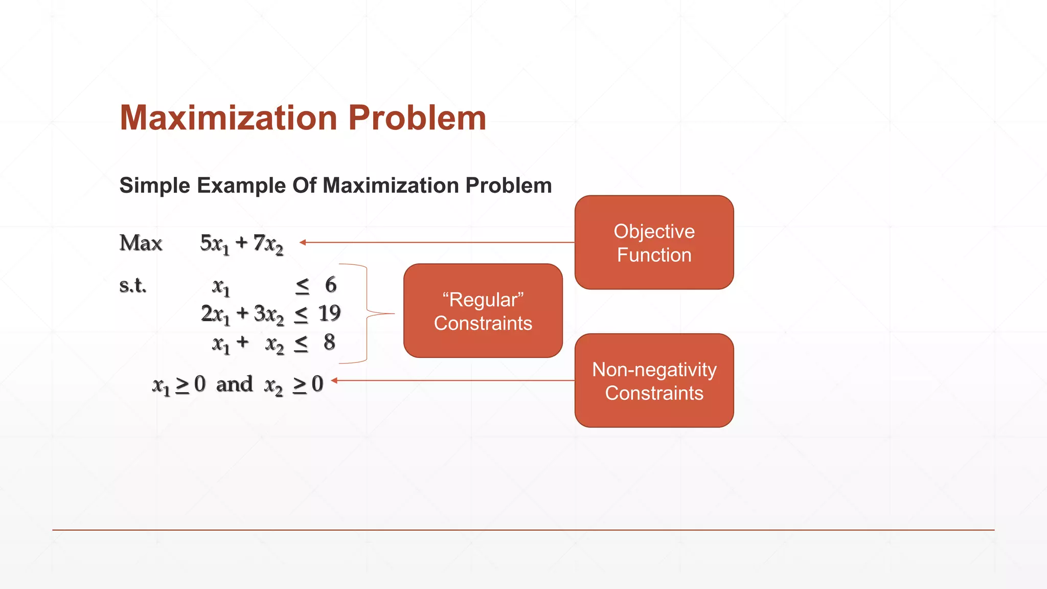
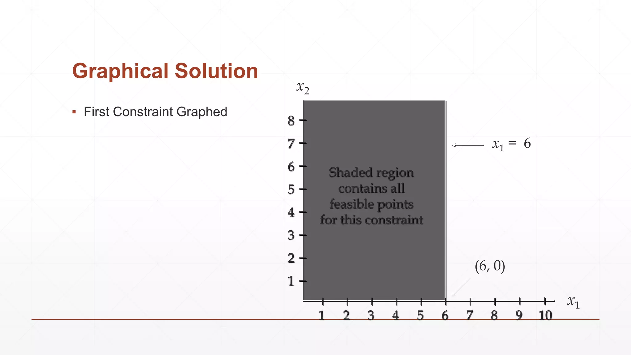
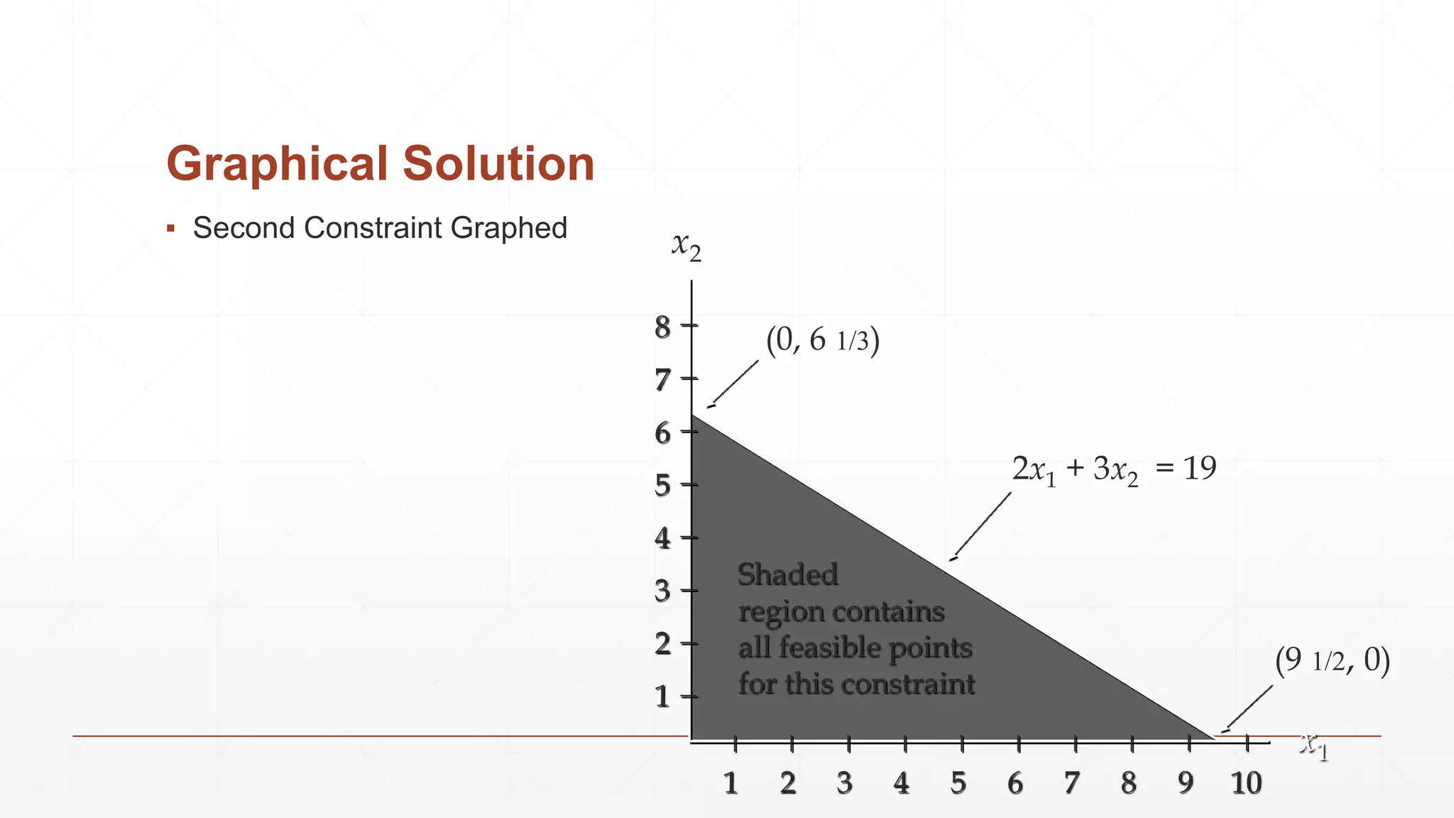
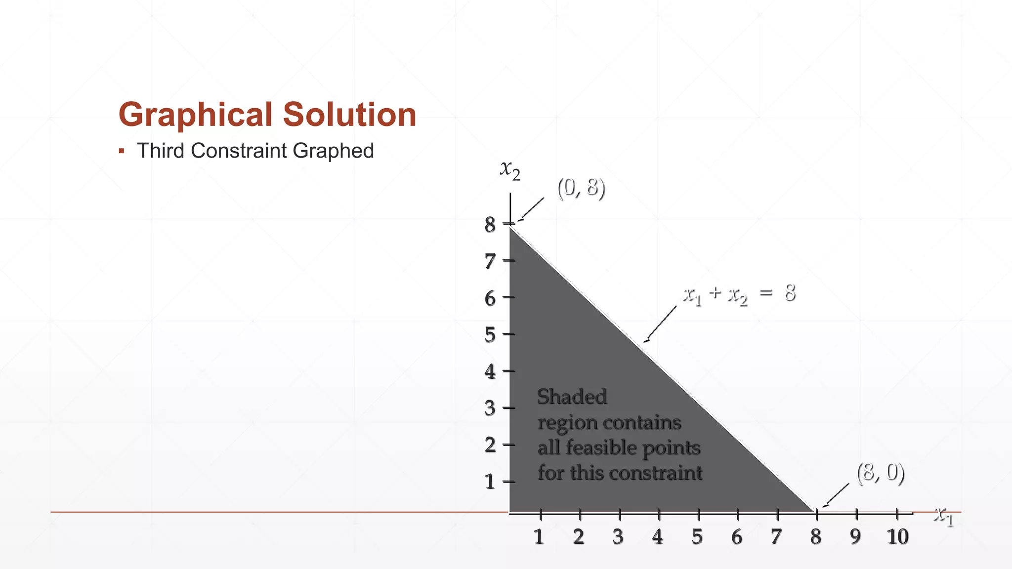
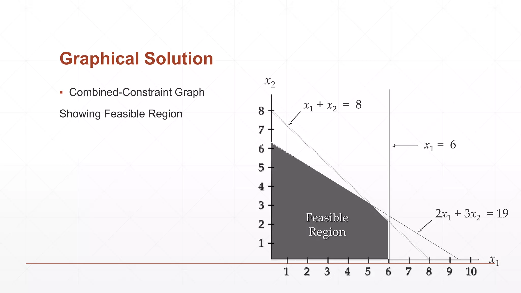
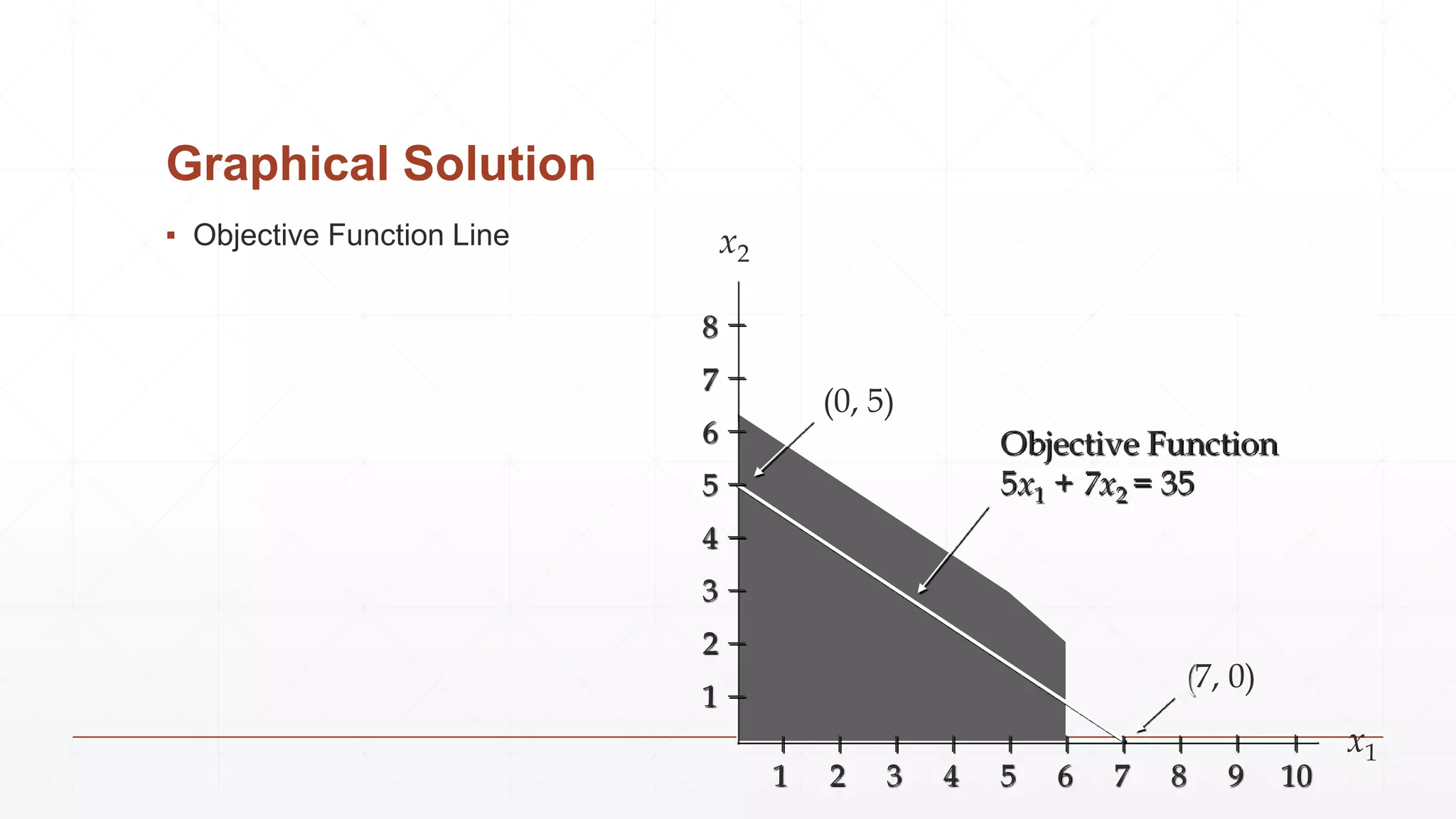
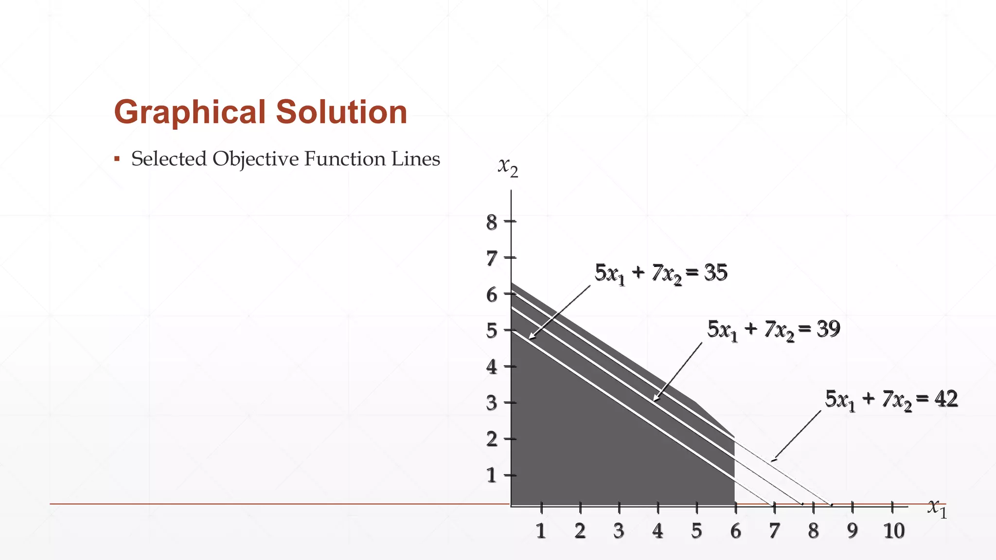
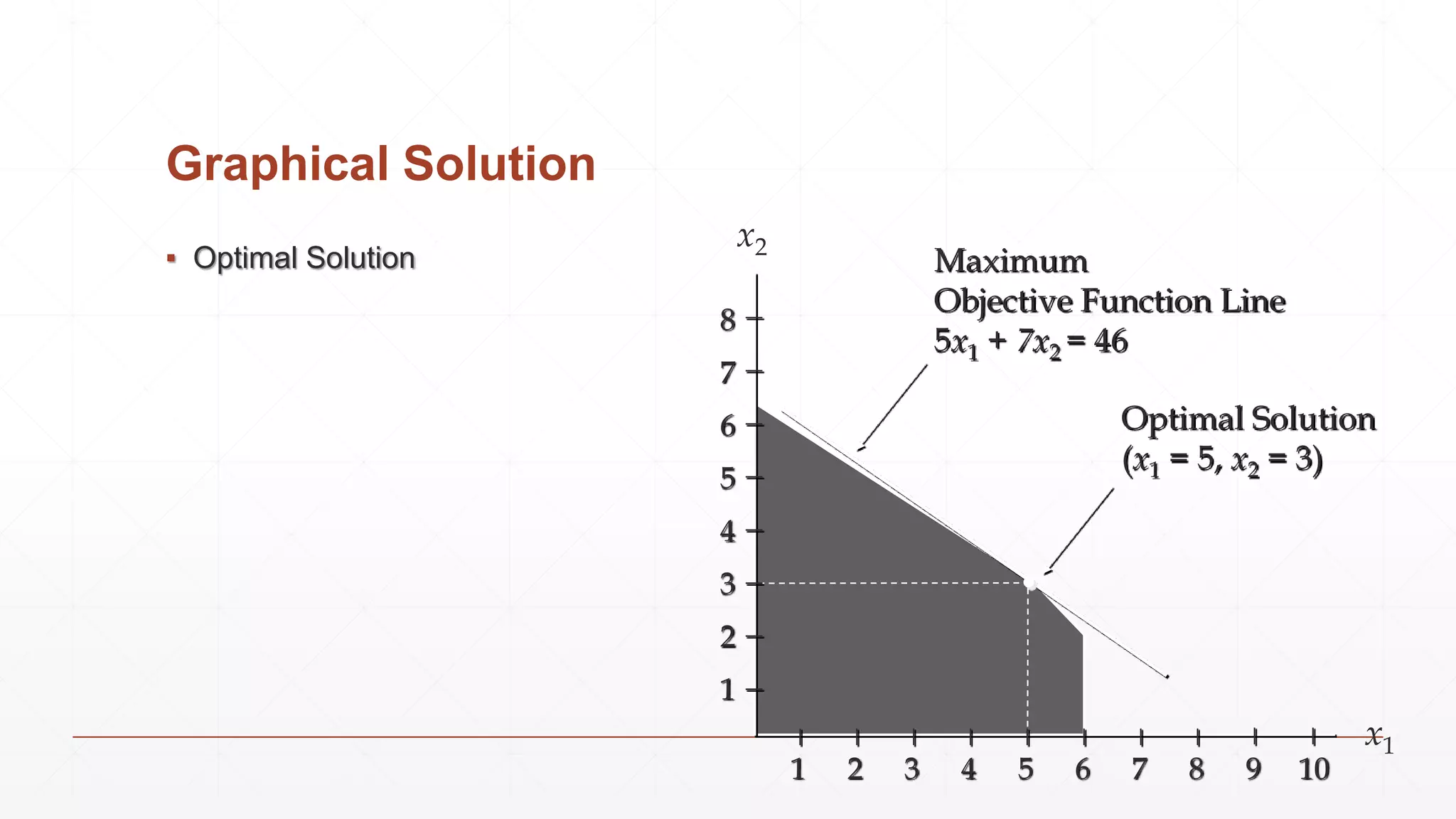
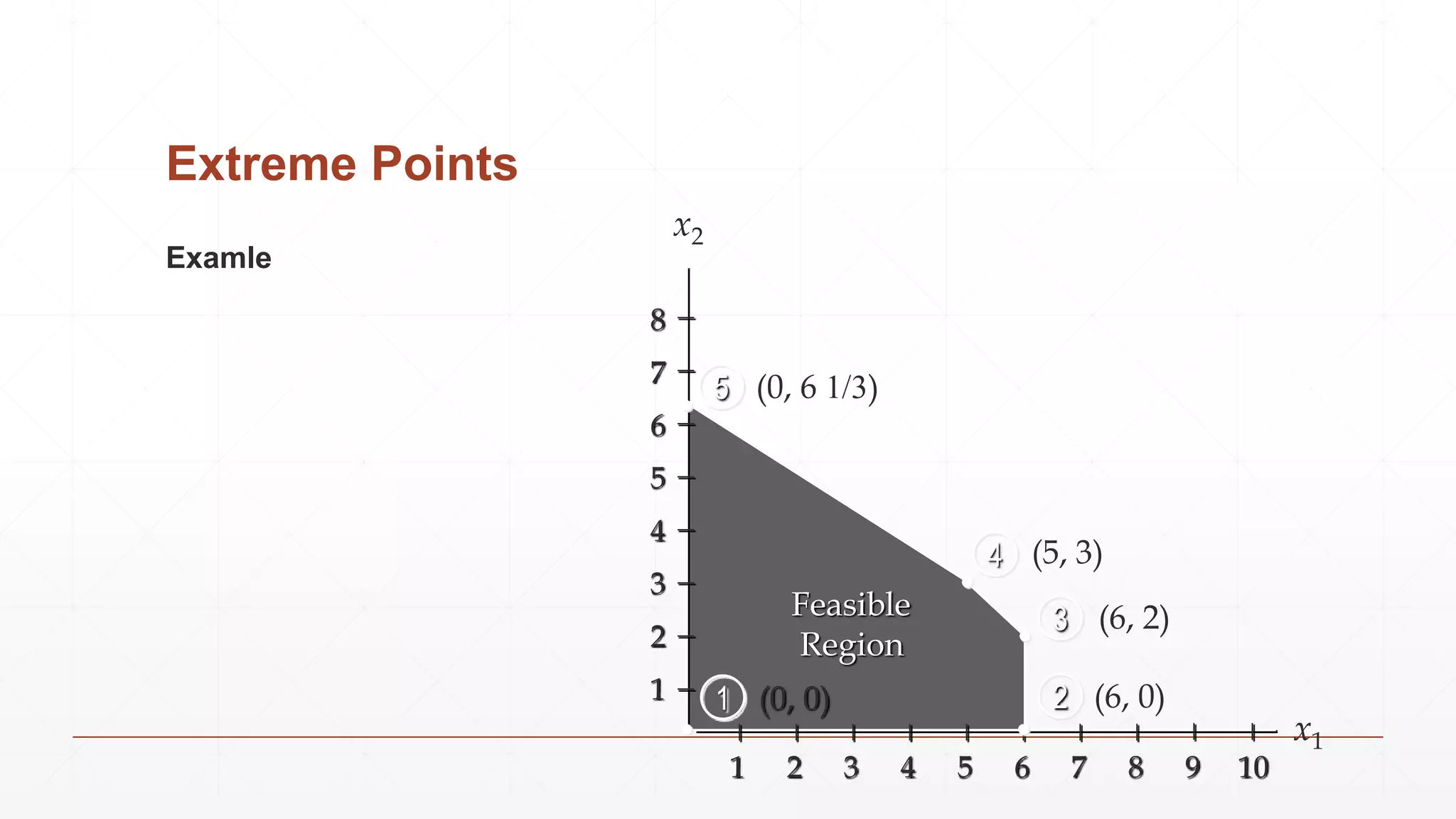
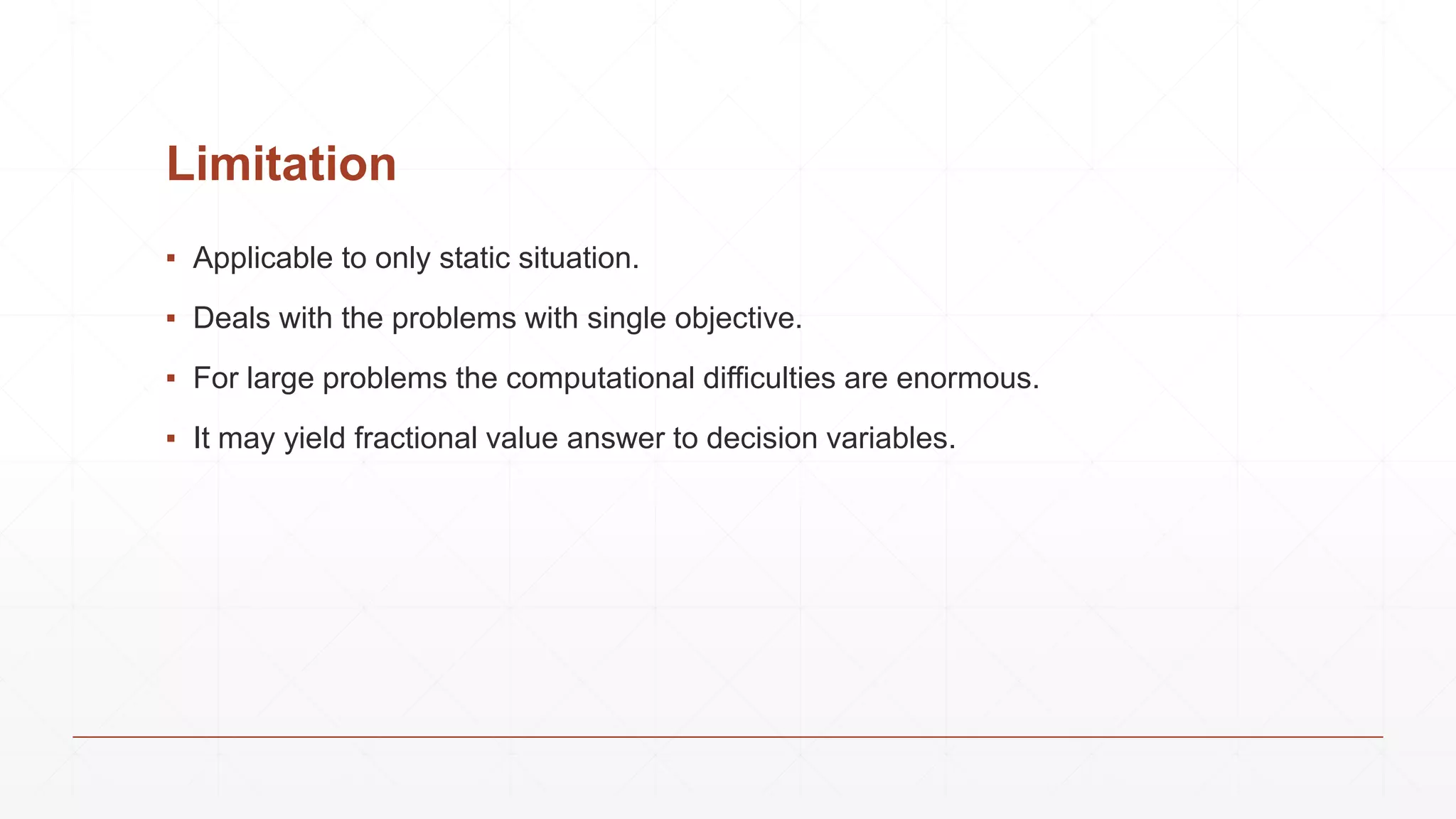
LINEAR
PROGRAMMING
RASHID ANSARI
170847980003
MTECH (ACDS)
INTRODUCTION
▪ Linear programming is a method to achieve the best outcome in a mathematical
model.
▪ It is a special case of mathematical programming.
▪ Use of “programming here means “choosing a course of action”.
▪ Linear programming involves choosing a course of action when the mathematical
model of the problem contains only linear functions.
Linear Programming (LP) Problem
▪ The maximization or minimization of some quantity is the objective in all linear
programming problems.
▪ All LP problems have constraints that limit the degree to which the objective can
be pursued.
▪ A feasible solution satisfies all the problem's constraints.
▪ An optimal solution is a feasible solution that results in the largest possible
objective function value when maximizing (or smallest when minimizing).
Linear Programming (LP) Problem
▪ Linear functions are functions in which each variable appears in a separate term
raised to the first power and is multiplied by a constant (which could be 0).
▪ Linear constraints are linear functions that are restricted to be "less than or equal
to", "equal to", or "greater than or equal to" a constant.
▪ If both the objective function and the constraints are linear, the problem is referred
to as a linear programming problem.
Problem Modelling
▪ Is the process of translating a verbal statement of a problem into a mathematical
statement.
▪ Every LP problems has some unique features, but most problems also have
common features.
Guidelines for Model Formulation
▪ Understand the problem thoroughly.
▪ Describe the objective.
▪ Describe each constraint.
▪ Define the decision variables.
▪ Write the objective in terms of the decision variables.
▪ Write the constraints in terms of the decision variables.
Graphical Solution Procedure
▪ Prepare a graph of the feasible solutions for each of the constraints.
▪ Determine the feasible region that satisfies all the constraints simultaneously.
▪ Draw an objective function line.
▪ Move parallel objective function lines toward larger objective function values
without entirely leaving the feasible region.
▪ Any feasible solution on the objective function line with the largest value is an
optimal solution.
Slack And Surplus Variables
▪ A linear program in which all the variables are non-negative and all the constraints are equalities is said to be in
standard form.
▪ Standard form is attained by adding slack variables to "less than or equal to" constraints, and by subtracting surplus
variables from "greater than or equal to" constraints.
▪ Slack and surplus variables represent the difference between the left and right sides of the constraints.
▪ Slack and surplus variables have objective function coefficients equal to 0.
Maximization Problem
Simple Example Of Maximization Problem
Max 5x1 + 7x2
s.t. x1 < 6
2x1 + 3x2 < 19
x1 + x2 < 8
x1 > 0 and x2 > 0
Objective
Function
“Regular”
Constraints
Non-negativity
Constraints
Graphical Solution
▪ First Constraint Graphed
x2
x1
x1 = 6
(6, 0)
8
7
6
5
4
3
2
1
1 2 3 4 5 6 7 8 9 10
Shaded region
contains all
feasible points
for this constraint
Graphical Solution
▪ Second Constraint Graphed
2x1 + 3x2 = 19
x2
x1
(0, 6 1/3)
(9 1/2, 0)
8
7
6
5
4
3
2
1
Shaded
region contains
all feasible points
for this constraint
1 2 3 4 5 6 7 8 9 10
Graphical Solution
▪ Third Constraint Graphed
x2
x1
x1 + x2 = 8
(0, 8)
(8, 0)
8
7
6
5
4
3
2
1
1 2 3 4 5 6 7 8 9 10
Shaded
region contains
all feasible points
for this constraint
Graphical Solution
▪ Combined-Constraint Graph
Showing Feasible Region
x1
x2
8
7
6
5
4
3
2
1
1 2 3 4 5 6 7 8 9 10
2x1 + 3x2 = 19
x1 + x2 = 8
x1 = 6
Feasible
Region
Graphical Solution
▪ Objective Function Line
x1
x2
(7, 0)
(0, 5)
Objective Function
5x1 + 7x2 = 35
8
7
6
5
4
3
2
1
1 2 3 4 5 6 7 8 9 10
Graphical Solution
▪ Selected Objective Function Lines
x1
x2
5x1 + 7x2 = 35
8
7
6
5
4
3
2
1
5x1 + 7x2 = 42
5x1 + 7x2 = 39
1 2 3 4 5 6 7 8 9 10
Graphical Solution
▪ Optimal Solution
x1
x2
Maximum
Objective Function Line
5x1 + 7x2 = 46
Optimal Solution
(x1 = 5, x2 = 3)
8
7
6
5
4
3
2
1
1 2 3 4 5 6 7 8 9 10
Extreme Points and the Optimal Solution
▪ The corners or vertices of the feasible region are referred to as the extreme
points.
▪ An optimal solution to an LP problem can be found at an extreme point of the
feasible region.
▪ When looking for the optimal solution, you do not have to evaluate all feasible
solution points.
▪ You have to consider only the extreme points of the feasible region.
Extreme Points
Examle
x1
Feasible
Region
1 2
3
4
5
x2
8
7
6
5
4
3
2
1
1 2 3 4 5 6 7 8 9 10
(0, 6 1/3)
(5, 3)
(0, 0)
(6, 2)
(6, 0)
Computer Solution
▪ LP problems involving 1000s of variables and 1000s of constraints are now
routinely solved with computer packages.
▪ Linear programming solvers are now part of many spreadsheet packages, such
as Microsoft Excel.
Application
▪ Business
▪ Industrial
▪ Military
▪ Marketing
Advantages
▪ Imroves the quality of the decisions
▪ Provides better tools for meeting the changing conditions.
▪ Highlights the bottleneck in the production process.
Limitation
▪ Applicable to only static situation.
▪ Deals with the problems with single objective.
▪ For large problems the computational difficulties are enormous.
▪ It may yield fractional value answer to decision variables.
References
LINKS
▪ https://en.wikipedia.org/wiki/Linear_programming
▪ https://faculty.mu.edu.sa/public
▪ https://www.slideshare.net/tiwarimanutiwari/linear-programing
THANK YOU

Linear Programming

  • 1.
  • 2.
    INTRODUCTION ▪ Linear programmingis a method to achieve the best outcome in a mathematical model. ▪ It is a special case of mathematical programming. ▪ Use of “programming here means “choosing a course of action”. ▪ Linear programming involves choosing a course of action when the mathematical model of the problem contains only linear functions.
  • 3.
    Linear Programming (LP)Problem ▪ The maximization or minimization of some quantity is the objective in all linear programming problems. ▪ All LP problems have constraints that limit the degree to which the objective can be pursued. ▪ A feasible solution satisfies all the problem's constraints. ▪ An optimal solution is a feasible solution that results in the largest possible objective function value when maximizing (or smallest when minimizing).
  • 4.
    Linear Programming (LP)Problem ▪ Linear functions are functions in which each variable appears in a separate term raised to the first power and is multiplied by a constant (which could be 0). ▪ Linear constraints are linear functions that are restricted to be "less than or equal to", "equal to", or "greater than or equal to" a constant. ▪ If both the objective function and the constraints are linear, the problem is referred to as a linear programming problem.
  • 5.
    Problem Modelling ▪ Isthe process of translating a verbal statement of a problem into a mathematical statement. ▪ Every LP problems has some unique features, but most problems also have common features.
  • 6.
    Guidelines for ModelFormulation ▪ Understand the problem thoroughly. ▪ Describe the objective. ▪ Describe each constraint. ▪ Define the decision variables. ▪ Write the objective in terms of the decision variables. ▪ Write the constraints in terms of the decision variables.
  • 7.
    Graphical Solution Procedure ▪Prepare a graph of the feasible solutions for each of the constraints. ▪ Determine the feasible region that satisfies all the constraints simultaneously. ▪ Draw an objective function line. ▪ Move parallel objective function lines toward larger objective function values without entirely leaving the feasible region. ▪ Any feasible solution on the objective function line with the largest value is an optimal solution.
  • 8.
    Slack And SurplusVariables ▪ A linear program in which all the variables are non-negative and all the constraints are equalities is said to be in standard form. ▪ Standard form is attained by adding slack variables to "less than or equal to" constraints, and by subtracting surplus variables from "greater than or equal to" constraints. ▪ Slack and surplus variables represent the difference between the left and right sides of the constraints. ▪ Slack and surplus variables have objective function coefficients equal to 0. ▪ A linear program in which all the variables are non-negative and all the constraints are equalities is said to be in standard form. ▪ Standard form is attained by adding slack variables to "less than or equal to" constraints, and by subtracting surplus variables from "greater than or equal to" constraints. ▪ Slack and surplus variables represent the difference between the left and right sides of the constraints. ▪ Slack and surplus variables have objective function coefficients equal to 0.
  • 9.
    Maximization Problem Simple ExampleOf Maximization Problem Max 5x1 + 7x2 s.t. x1 < 6 2x1 + 3x2 < 19 x1 + x2 < 8 x1 > 0 and x2 > 0 Objective Function “Regular” Constraints Non-negativity Constraints
  • 10.
    Graphical Solution ▪ FirstConstraint Graphed x2 x1 x1 = 6 (6, 0) 8 7 6 5 4 3 2 1 1 2 3 4 5 6 7 8 9 10 Shaded region contains all feasible points for this constraint
  • 11.
    Graphical Solution ▪ SecondConstraint Graphed 2x1 + 3x2 = 19 x2 x1 (0, 6 1/3) (9 1/2, 0) 8 7 6 5 4 3 2 1 Shaded region contains all feasible points for this constraint 1 2 3 4 5 6 7 8 9 10
  • 12.
    Graphical Solution ▪ ThirdConstraint Graphed x2 x1 x1 + x2 = 8 (0, 8) (8, 0) 8 7 6 5 4 3 2 1 1 2 3 4 5 6 7 8 9 10 Shaded region contains all feasible points for this constraint
  • 13.
    Graphical Solution ▪ Combined-ConstraintGraph Showing Feasible Region x1 x2 8 7 6 5 4 3 2 1 1 2 3 4 5 6 7 8 9 10 2x1 + 3x2 = 19 x1 + x2 = 8 x1 = 6 Feasible Region
  • 14.
    Graphical Solution ▪ ObjectiveFunction Line x1 x2 (7, 0) (0, 5) Objective Function 5x1 + 7x2 = 35 8 7 6 5 4 3 2 1 1 2 3 4 5 6 7 8 9 10
  • 15.
    Graphical Solution ▪ SelectedObjective Function Lines x1 x2 5x1 + 7x2 = 35 8 7 6 5 4 3 2 1 5x1 + 7x2 = 42 5x1 + 7x2 = 39 1 2 3 4 5 6 7 8 9 10
  • 16.
    Graphical Solution ▪ OptimalSolution x1 x2 Maximum Objective Function Line 5x1 + 7x2 = 46 Optimal Solution (x1 = 5, x2 = 3) 8 7 6 5 4 3 2 1 1 2 3 4 5 6 7 8 9 10
  • 17.
    Extreme Points andthe Optimal Solution ▪ The corners or vertices of the feasible region are referred to as the extreme points. ▪ An optimal solution to an LP problem can be found at an extreme point of the feasible region. ▪ When looking for the optimal solution, you do not have to evaluate all feasible solution points. ▪ You have to consider only the extreme points of the feasible region.
  • 18.
    Extreme Points Examle x1 Feasible Region 1 2 3 4 5 x2 8 7 6 5 4 3 2 1 12 3 4 5 6 7 8 9 10 (0, 6 1/3) (5, 3) (0, 0) (6, 2) (6, 0)
  • 19.
    Computer Solution ▪ LPproblems involving 1000s of variables and 1000s of constraints are now routinely solved with computer packages. ▪ Linear programming solvers are now part of many spreadsheet packages, such as Microsoft Excel.
  • 20.
  • 21.
    Advantages ▪ Imroves thequality of the decisions ▪ Provides better tools for meeting the changing conditions. ▪ Highlights the bottleneck in the production process.
  • 22.
    Limitation ▪ Applicable toonly static situation. ▪ Deals with the problems with single objective. ▪ For large problems the computational difficulties are enormous. ▪ It may yield fractional value answer to decision variables.
  • 23.
  • 24.