Download as PDF, PPTX
![Measure of Impurity: GINI
• Gini Index for a given node t :
• p( j | t) is the relative frequency of class j at node t.
– Maximum (1 - 1/nc) when records are equally
distributed among all classes, implying least
interesting information
– Minimum (0.0) when all records belong to one class,
implying most interesting information
j
tjptGINI 2
)]|([1)(](https://image.slidesharecdn.com/3-300310-160831222500/75/Machine-Learning-An-introduction-18-2048.jpg)
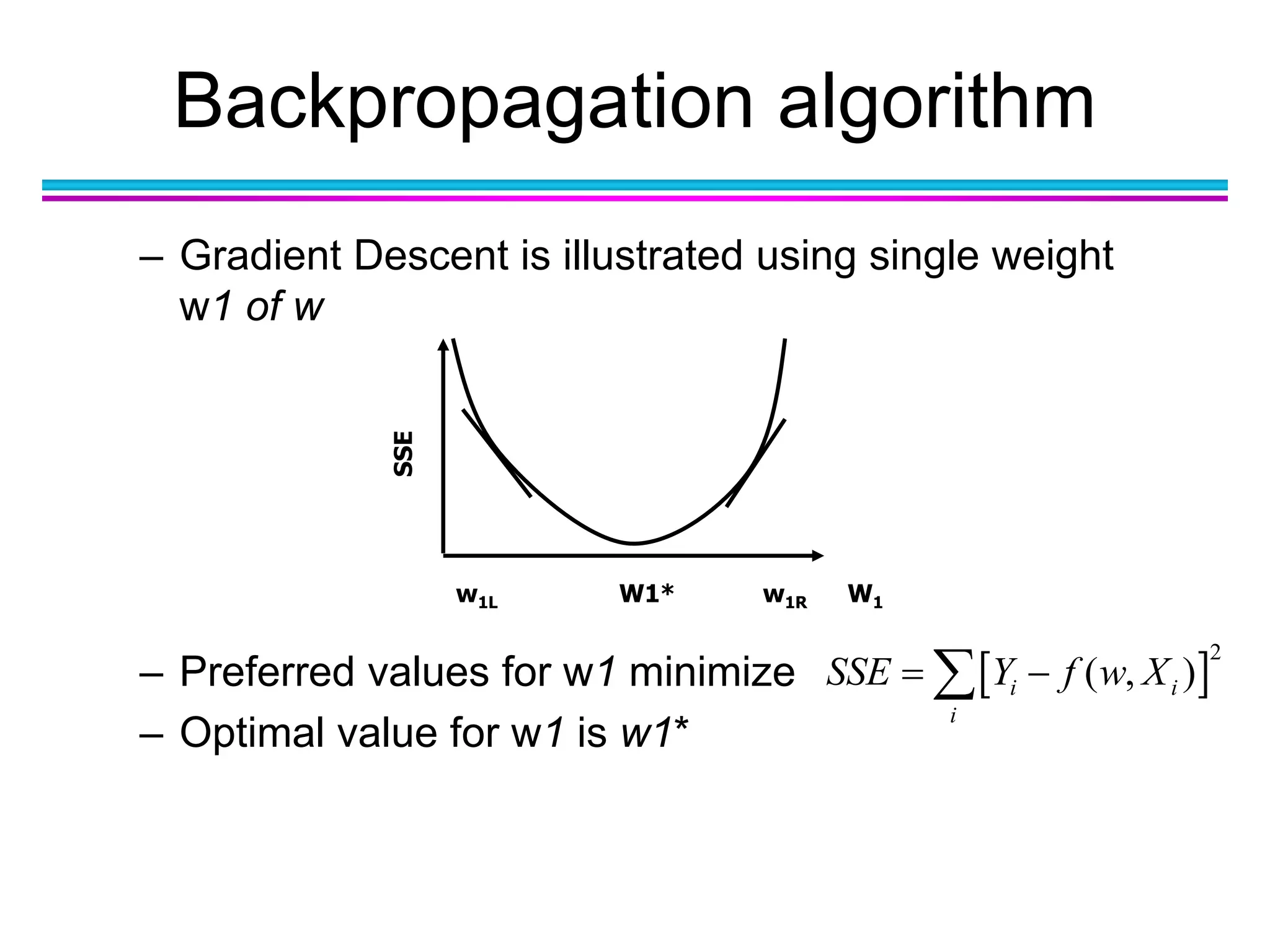
![Backpropagation algorithm
– Direction for adjusting wCURRENT is negative sign of
derivative at SSE at wCURRENT
– To adjust, use magnitude of the derivative of SSE at
wCURRENT
– When curve steep, adjustment large
– When curve nearly flat, adjustment small
– Learning Rate η has values [0, 1]
)(
CURRENTw
SSE
sign
)(
CURRENT
CURRENT
w
SSE
w
](https://image.slidesharecdn.com/3-300310-160831222500/75/Machine-Learning-An-introduction-29-2048.jpg)


![Measure of Impurity: GINI
• Gini Index for a given node t :
• p( j | t) is the relative frequency of class j at node t.
– Maximum (1 - 1/nc) when records are equally
distributed among all classes, implying least
interesting information
– Minimum (0.0) when all records belong to one class,
implying most interesting information
j
tjptGINI 2
)]|([1)(](https://crownmelresort.com/image.slidesharecdn.com/3-300310-160831222500/75/Machine-Learning-An-introduction-18-2048.jpg)


![Backpropagation algorithm
– Direction for adjusting wCURRENT is negative sign of
derivative at SSE at wCURRENT
– To adjust, use magnitude of the derivative of SSE at
wCURRENT
– When curve steep, adjustment large
– When curve nearly flat, adjustment small
– Learning Rate η has values [0, 1]
)(
CURRENTw
SSE
sign
)(
CURRENT
CURRENT
w
SSE
w
](https://crownmelresort.com/image.slidesharecdn.com/3-300310-160831222500/75/Machine-Learning-An-introduction-29-2048.jpg)


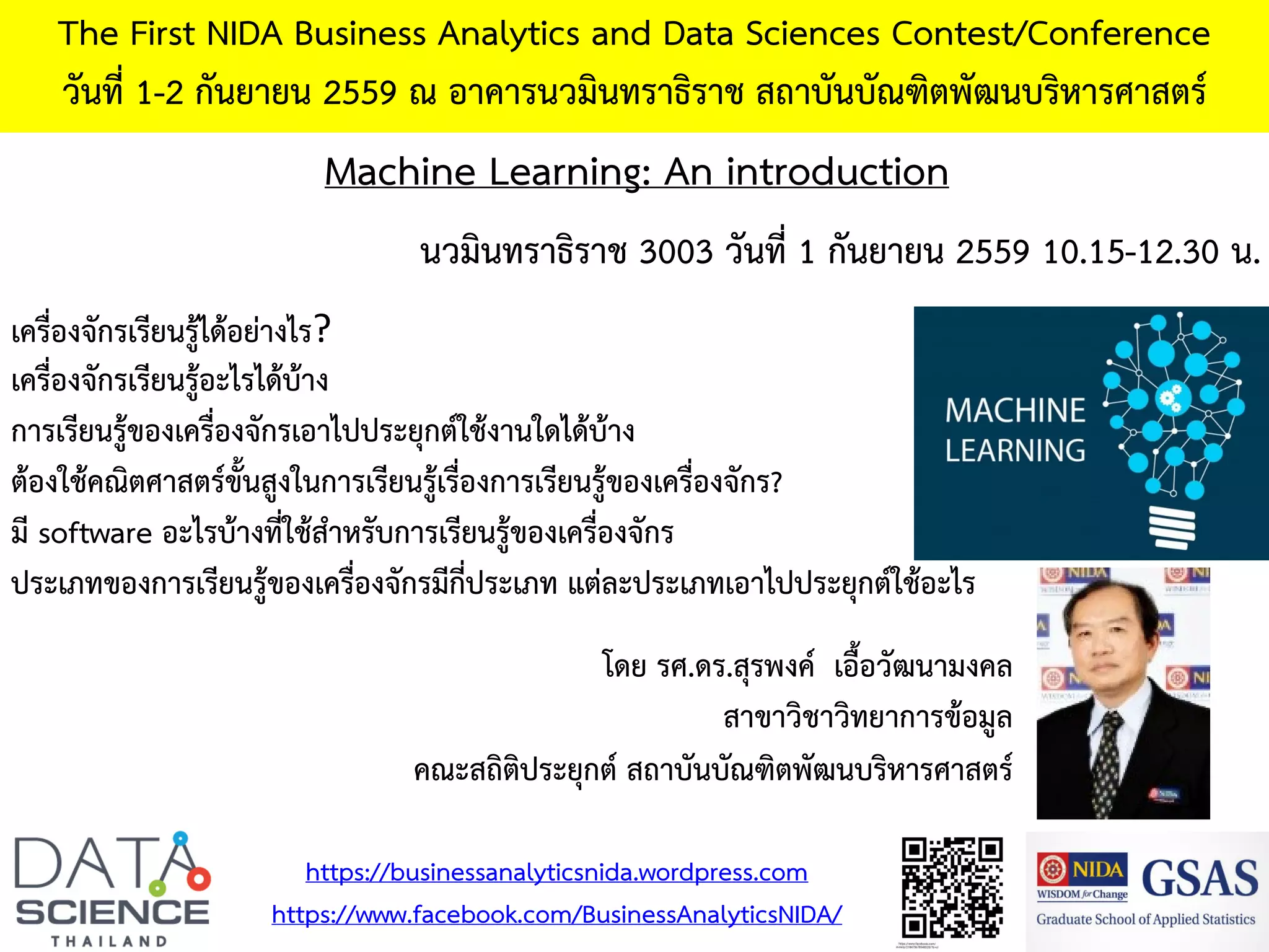
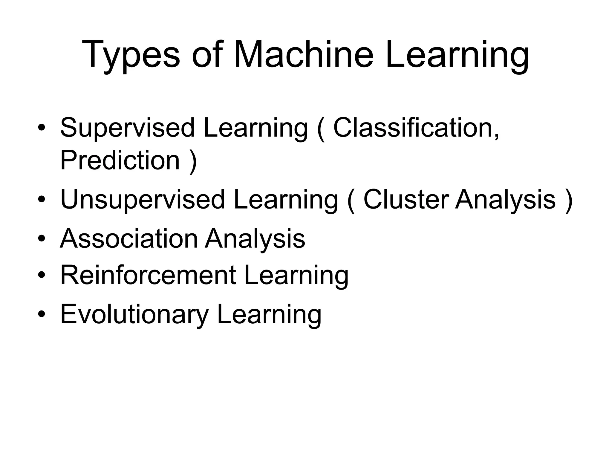
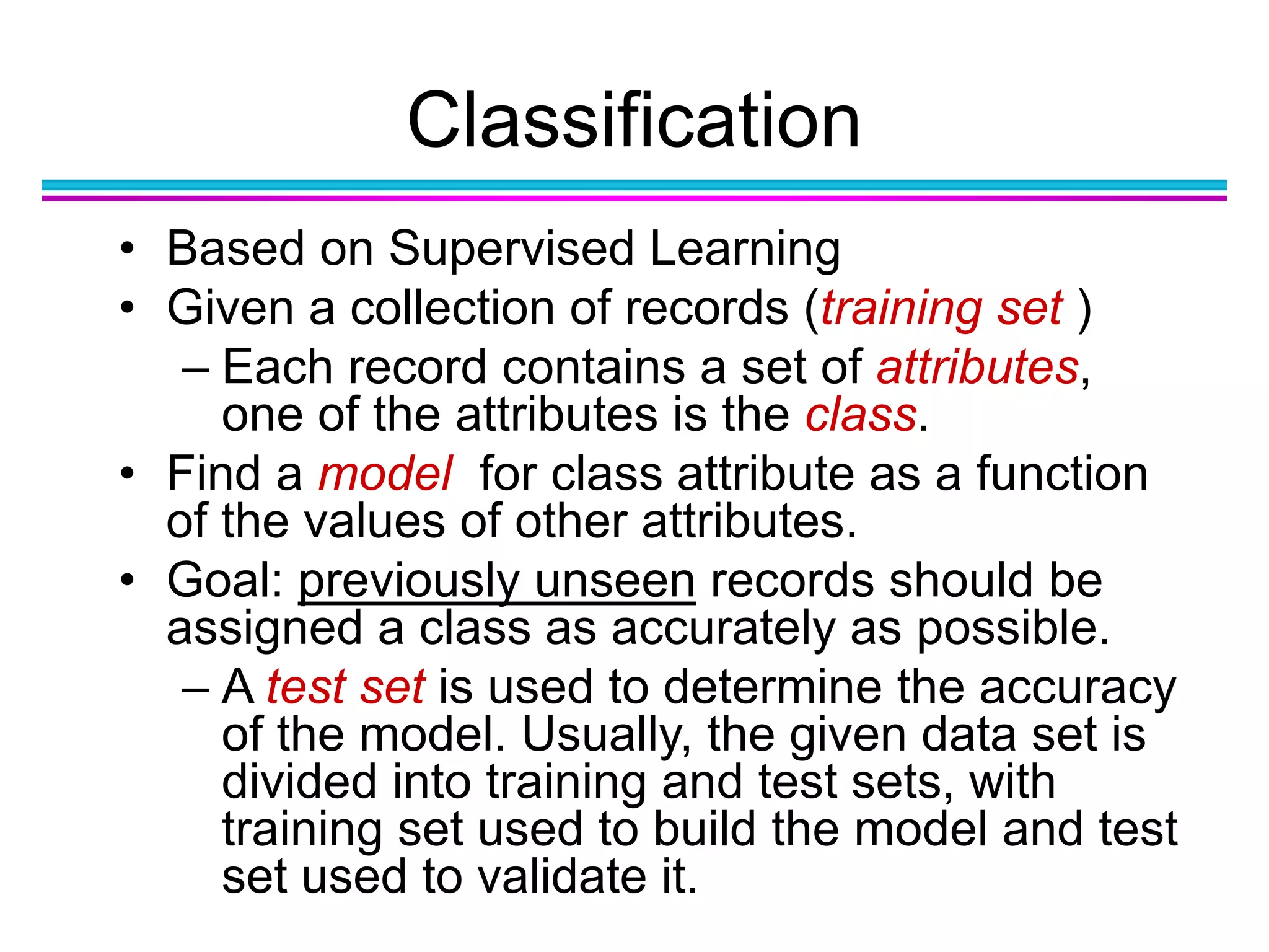
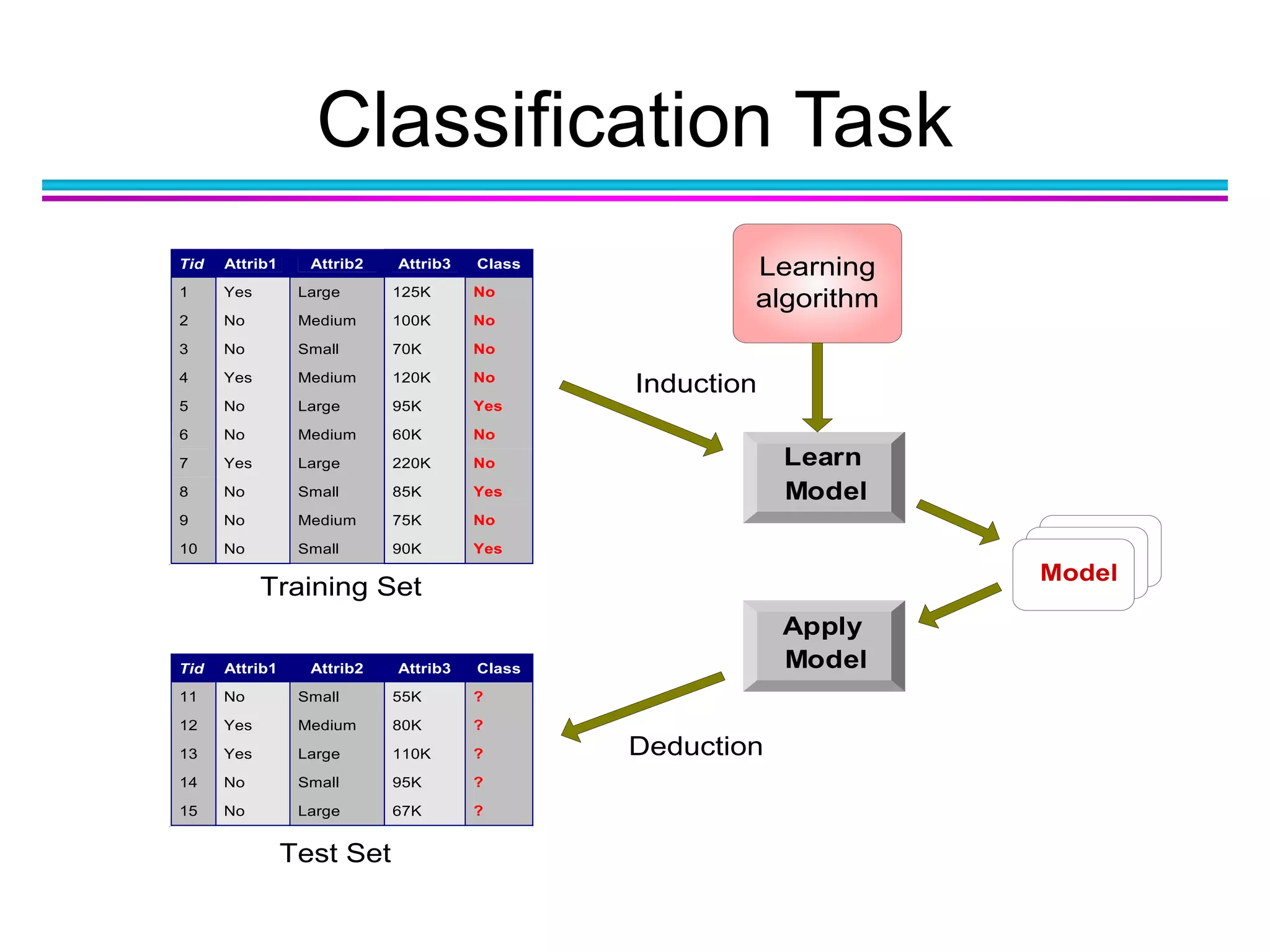
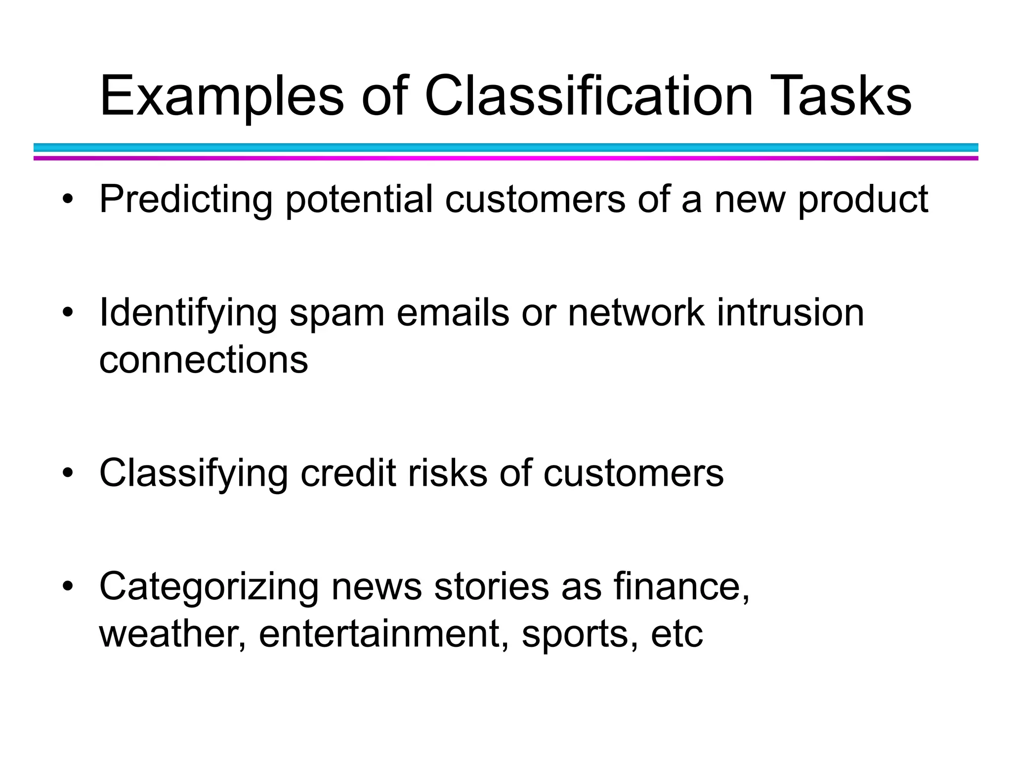
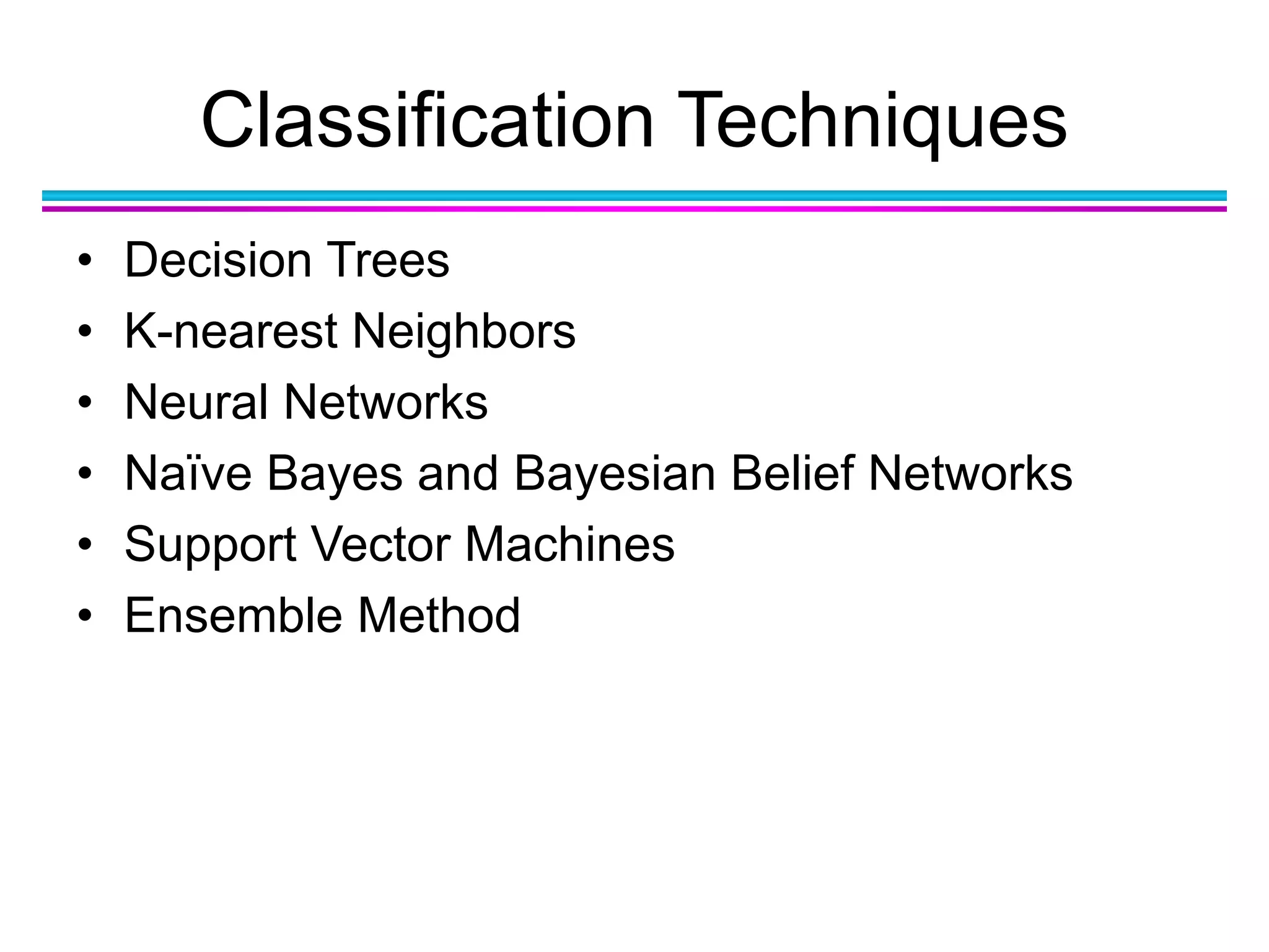
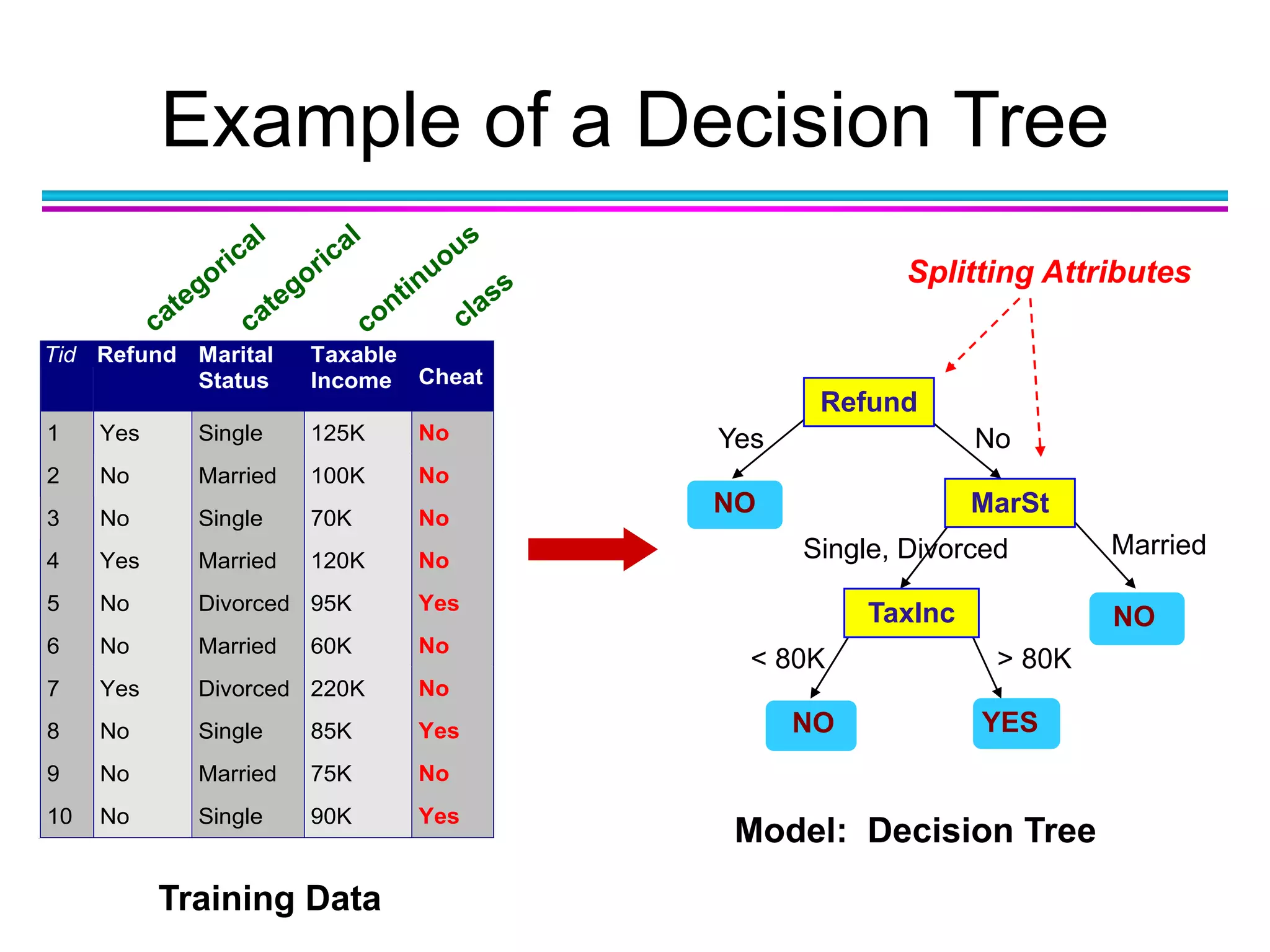
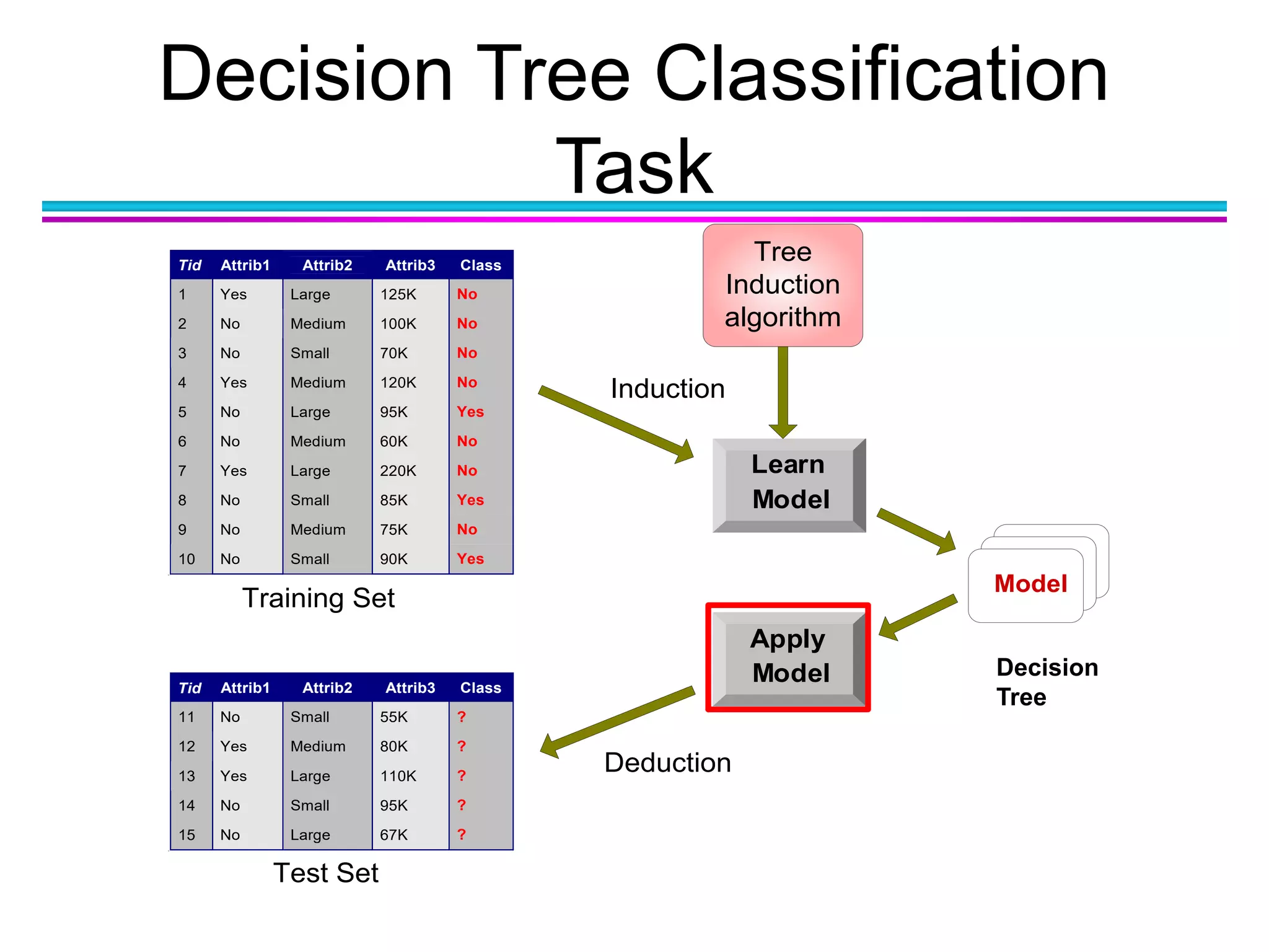
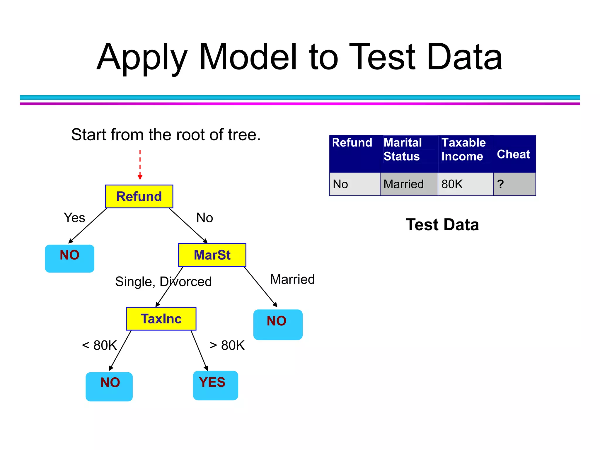
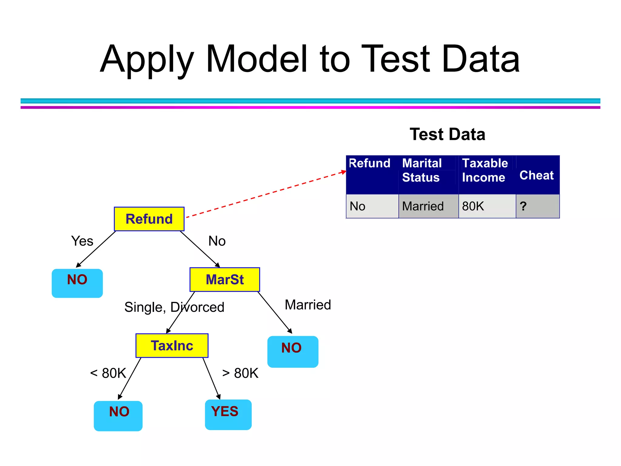
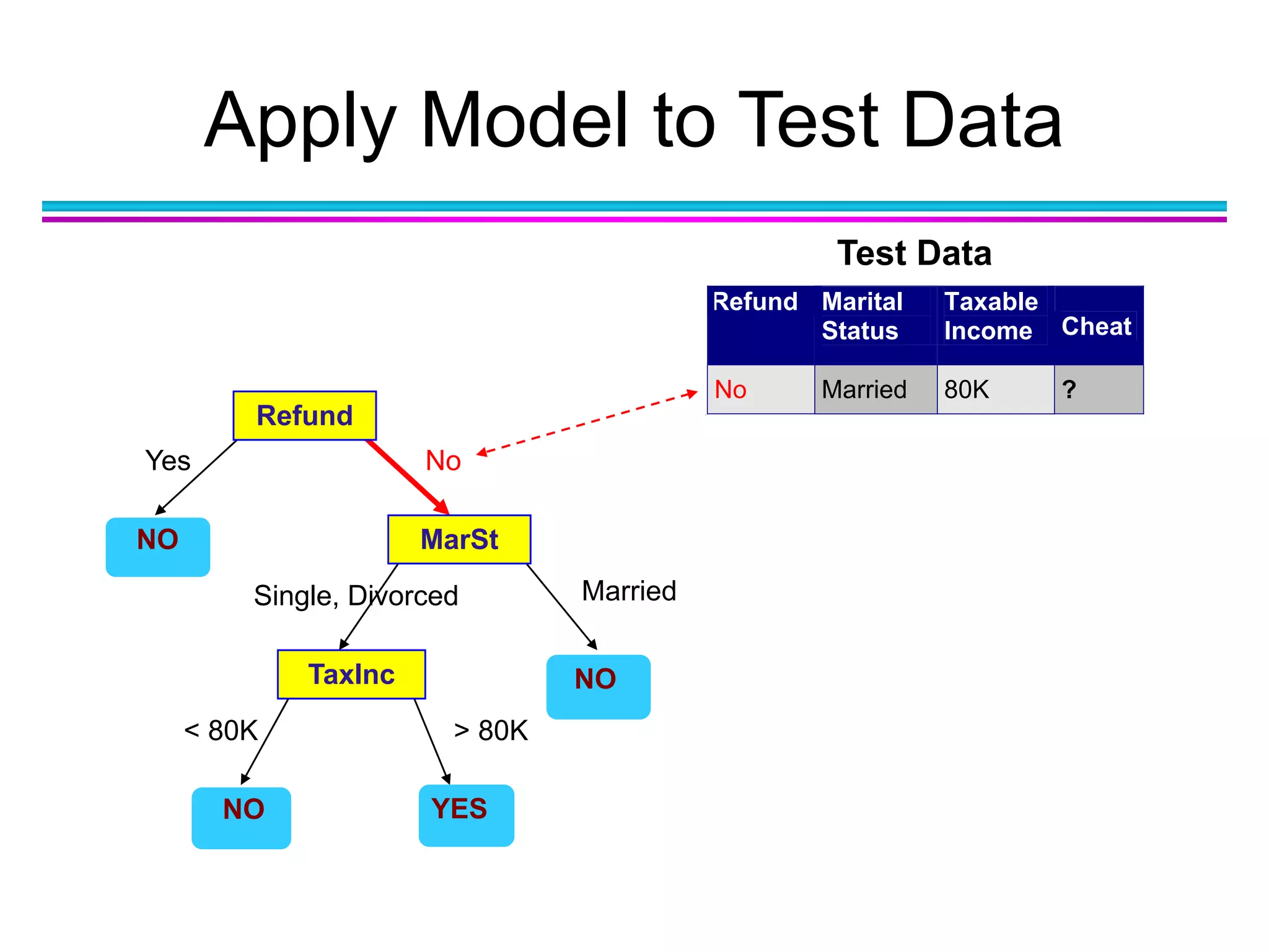
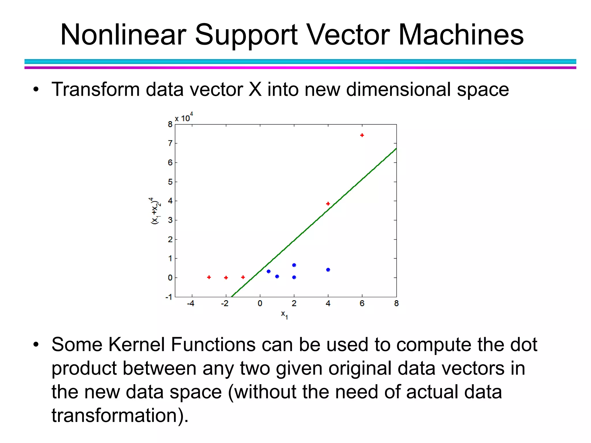
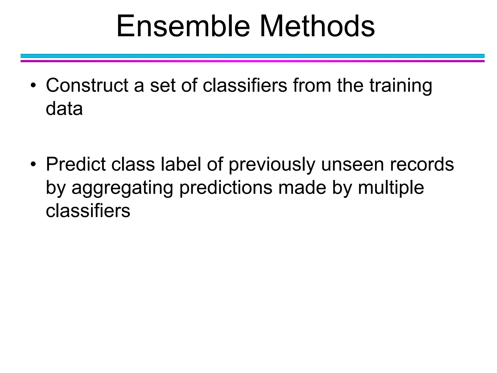
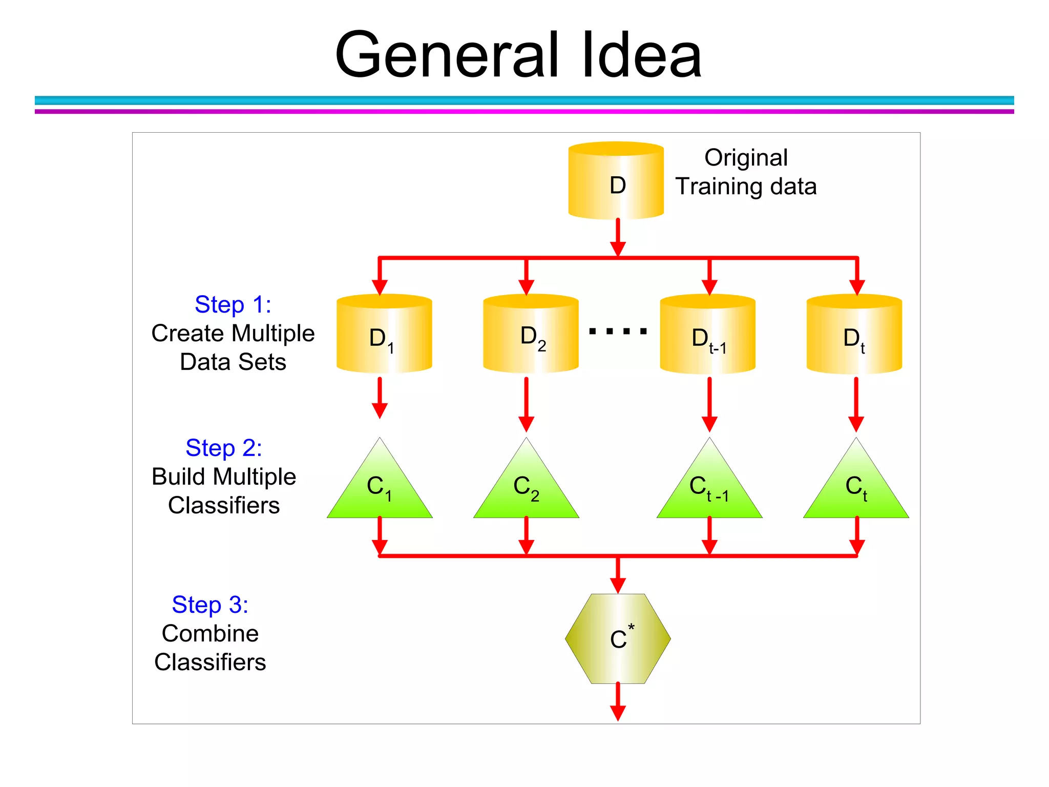
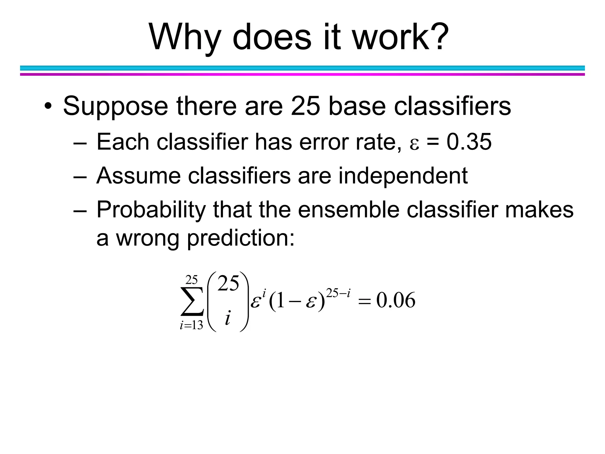
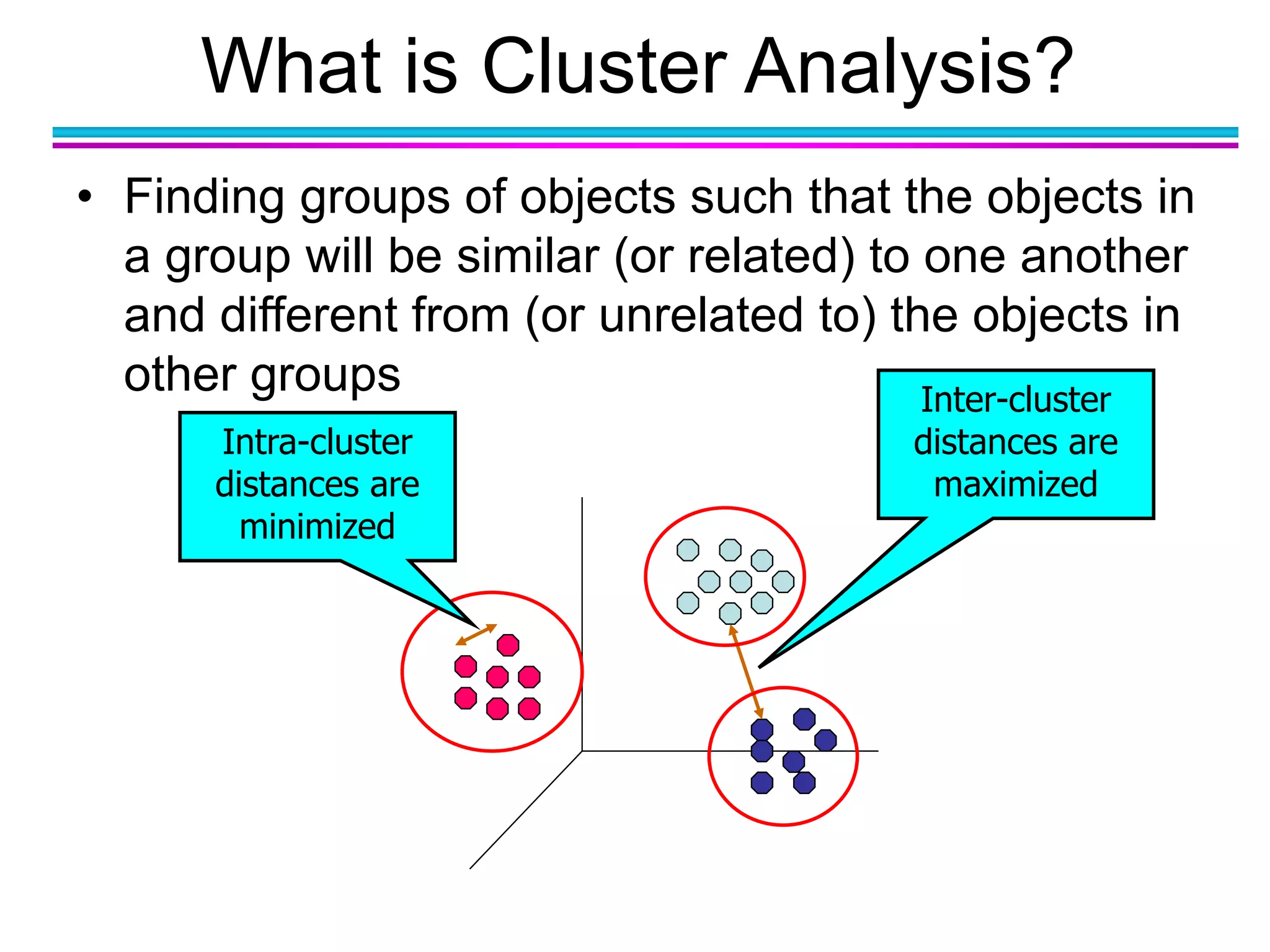
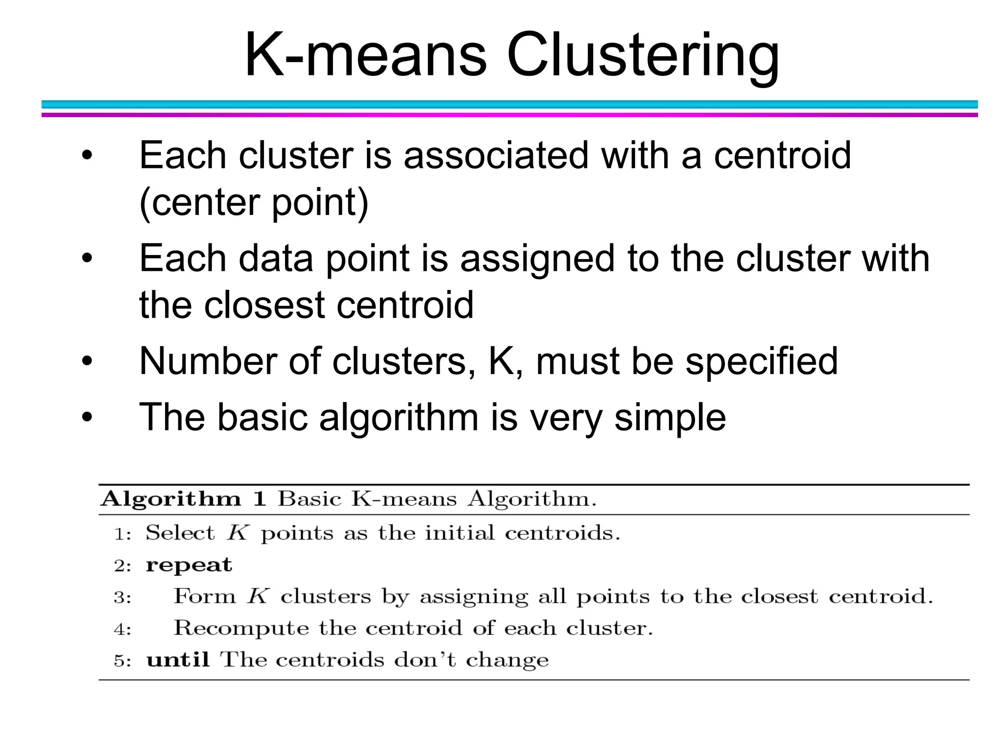
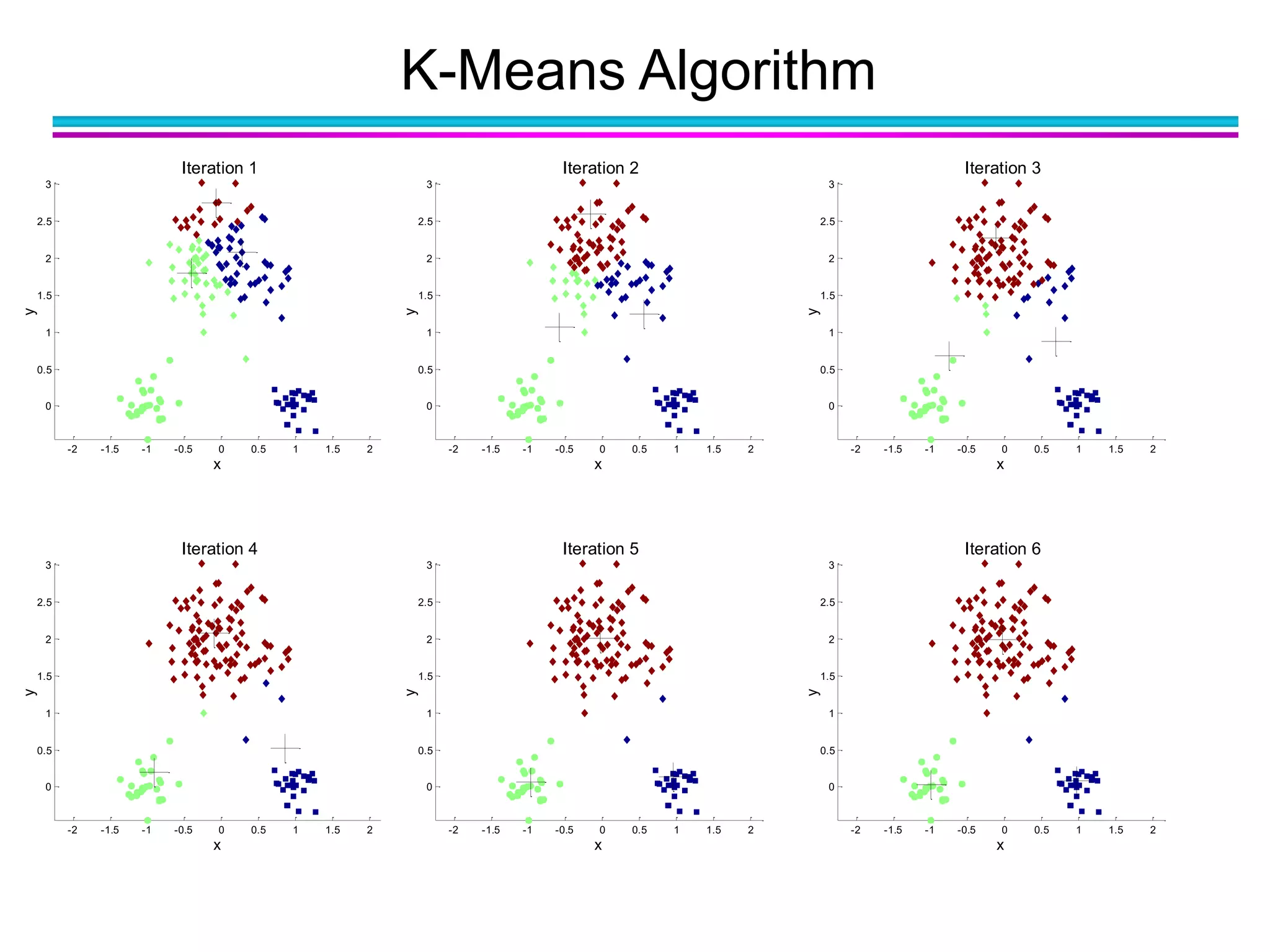
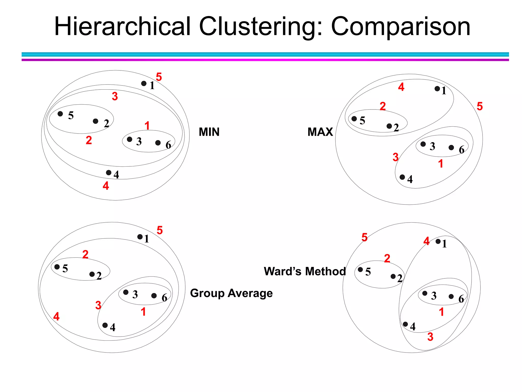
The document discusses the first NIDA Business Analytics and Data Sciences contest, focusing on machine learning, its types, and applications. It elaborates on techniques used in classification, such as decision trees, k-nearest neighbors, and support vector machines, alongside methods for clustering and ensemble learning. The document serves as an introductory guide to various machine learning algorithms and their practical uses in data analysis.


![[ppt]](https://cdn.slidesharecdn.com/ss_thumbnails/ppt2931-thumbnail.jpg?width=640&height=640&fit=bounds)
![[ppt]](https://cdn.slidesharecdn.com/ss_thumbnails/ppt3441-thumbnail.jpg?width=640&height=640&fit=bounds)


![SHS_Core_CAE_Q3_LE1 FOR THIRD [FINAL].pdf](https://cdn.slidesharecdn.com/ss_thumbnails/shscorecaeq3le1final-251116055110-e3081055-thumbnail.jpg?width=640&height=640&fit=bounds)


