Unit-4 classification

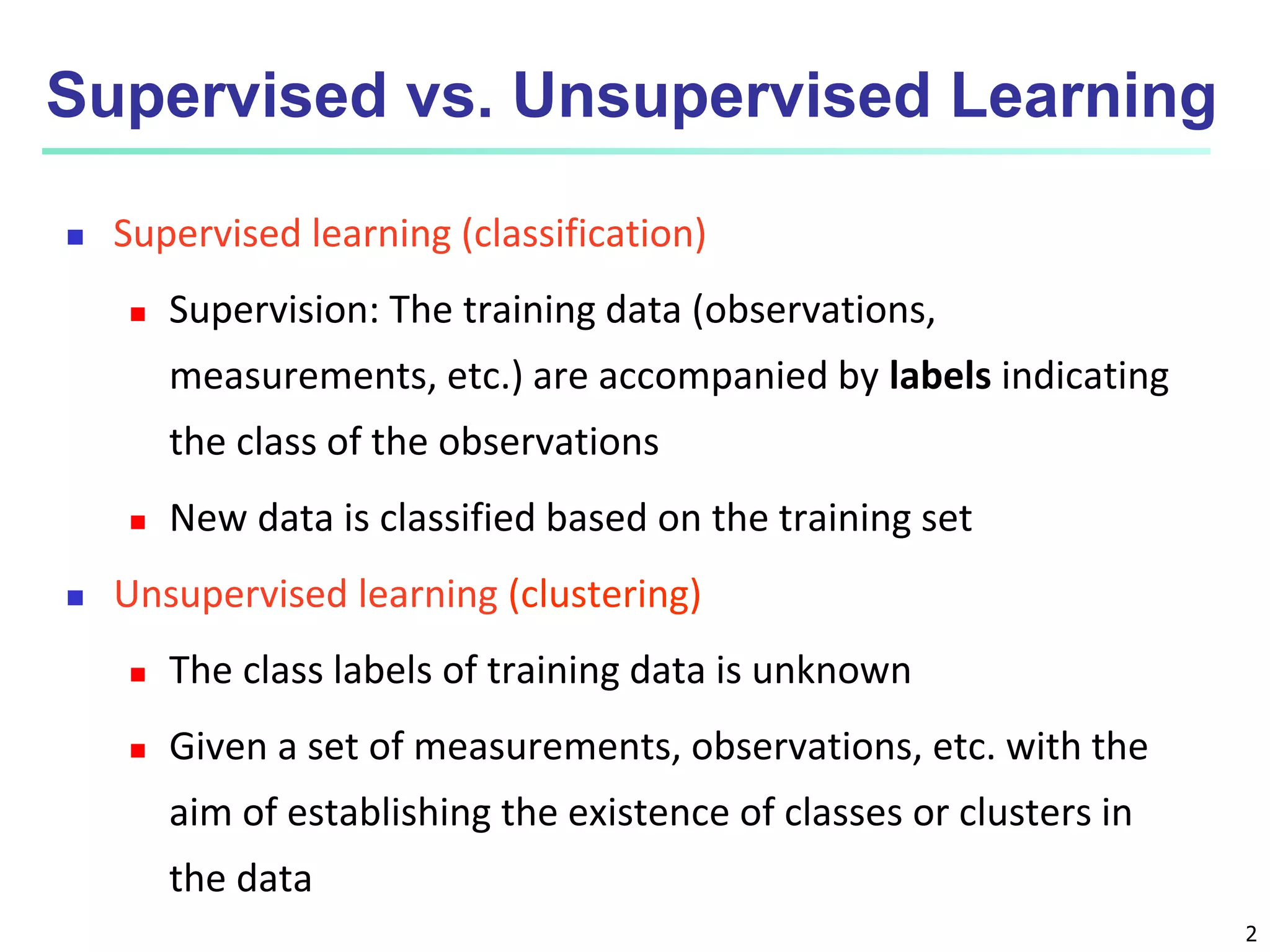
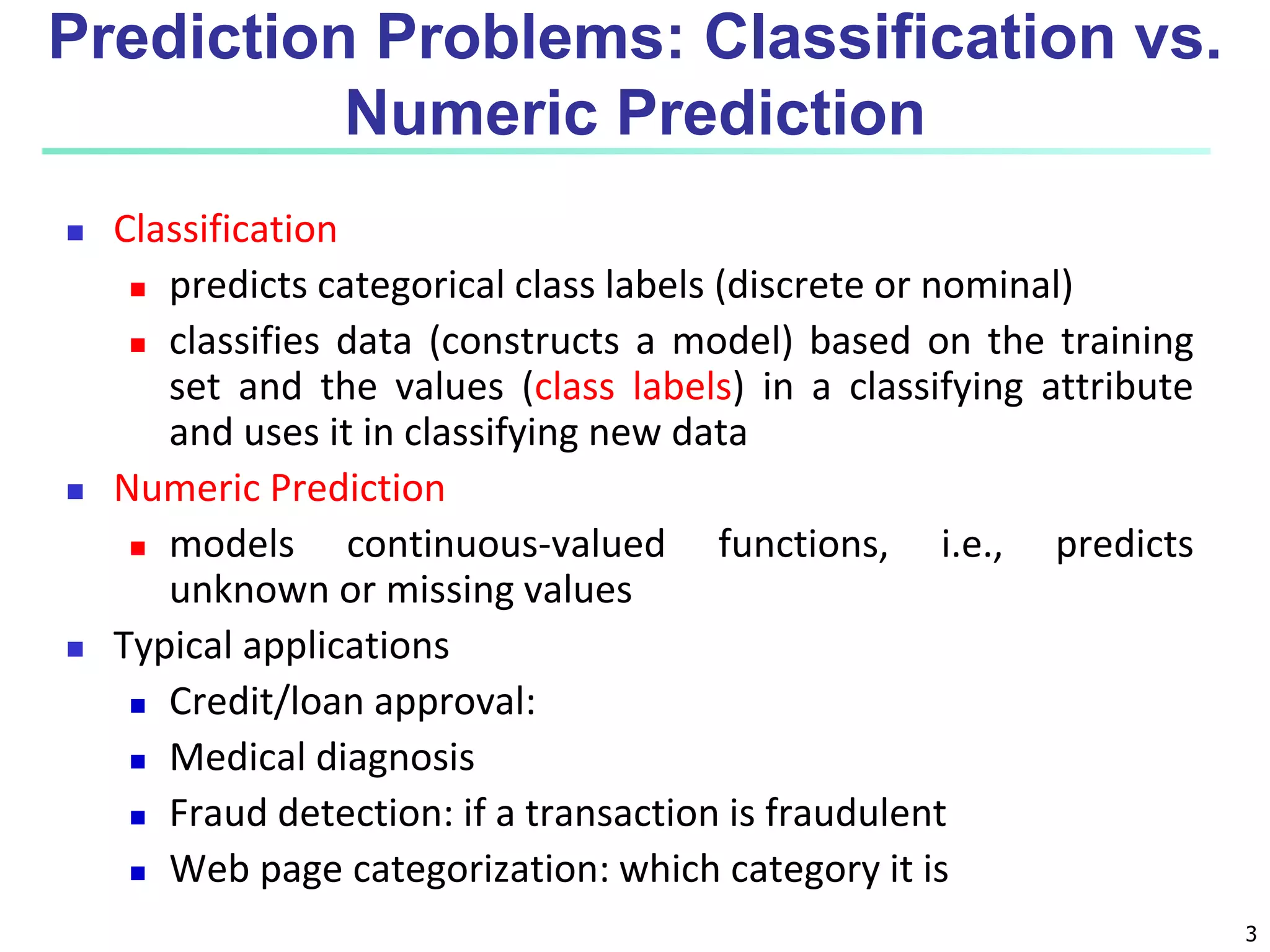
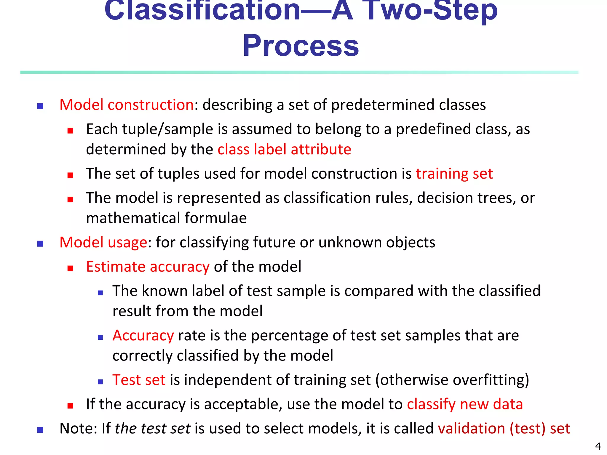
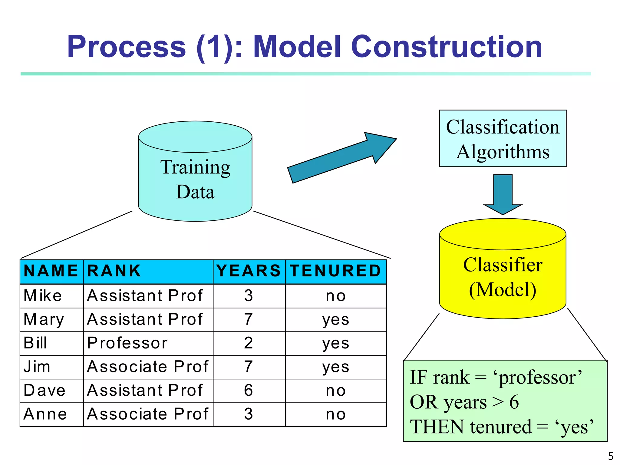
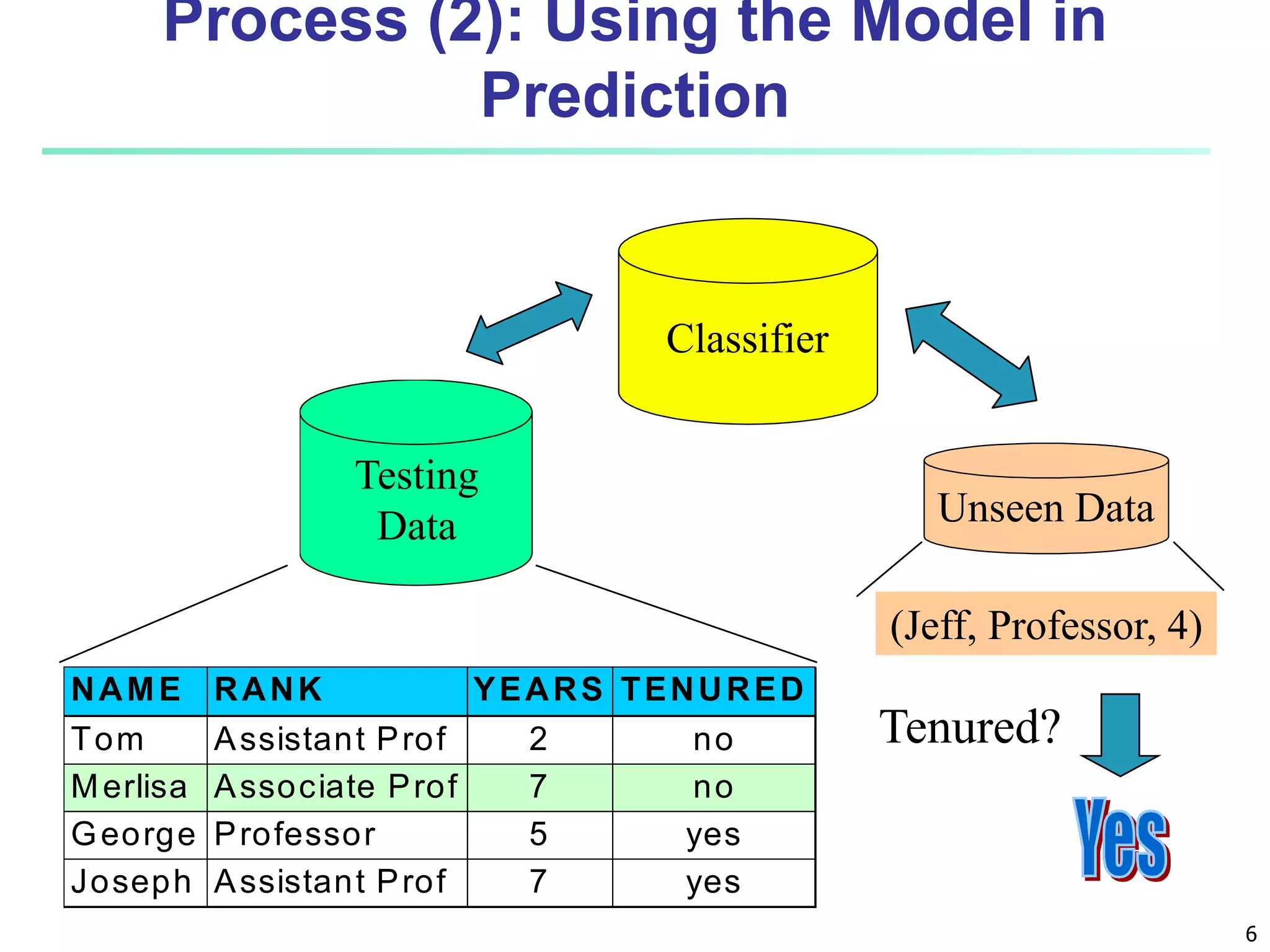
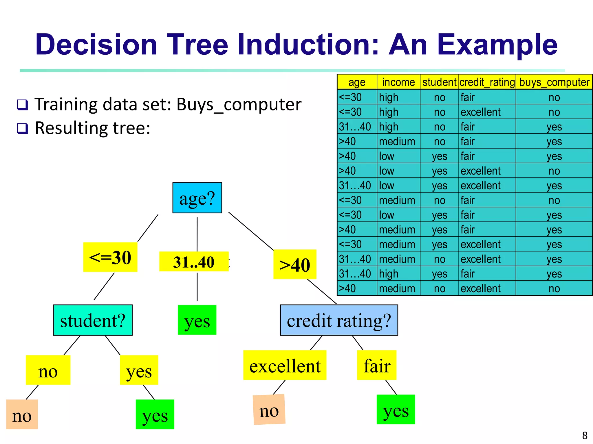
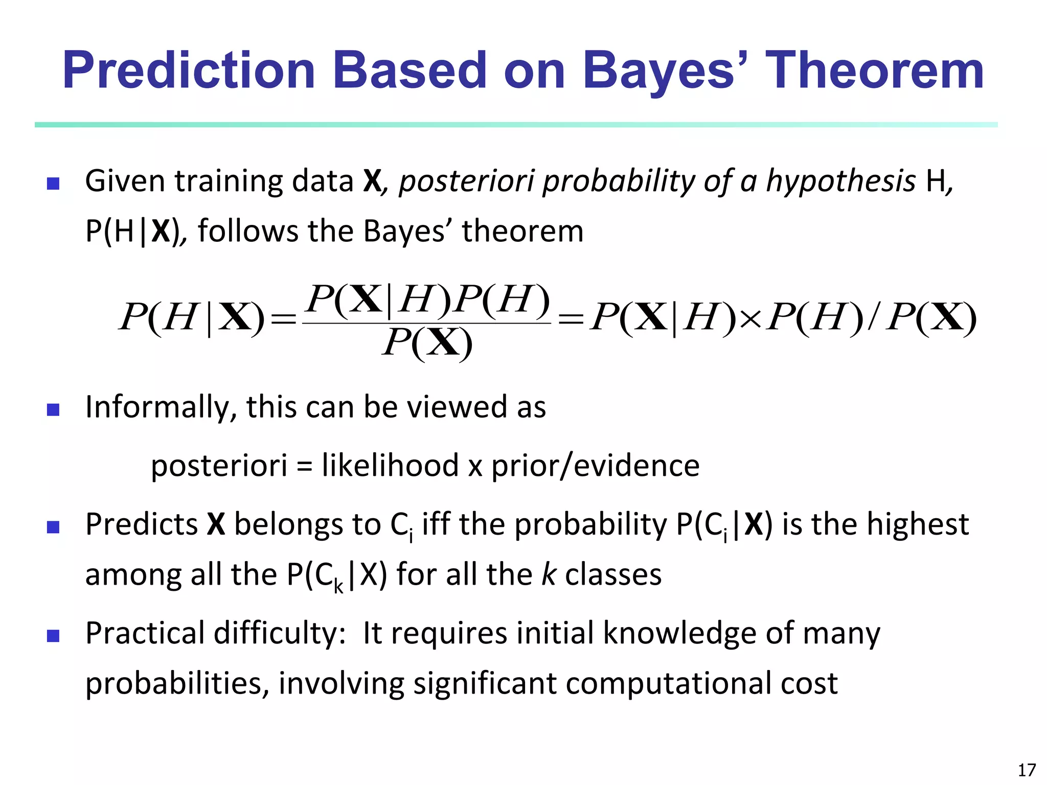
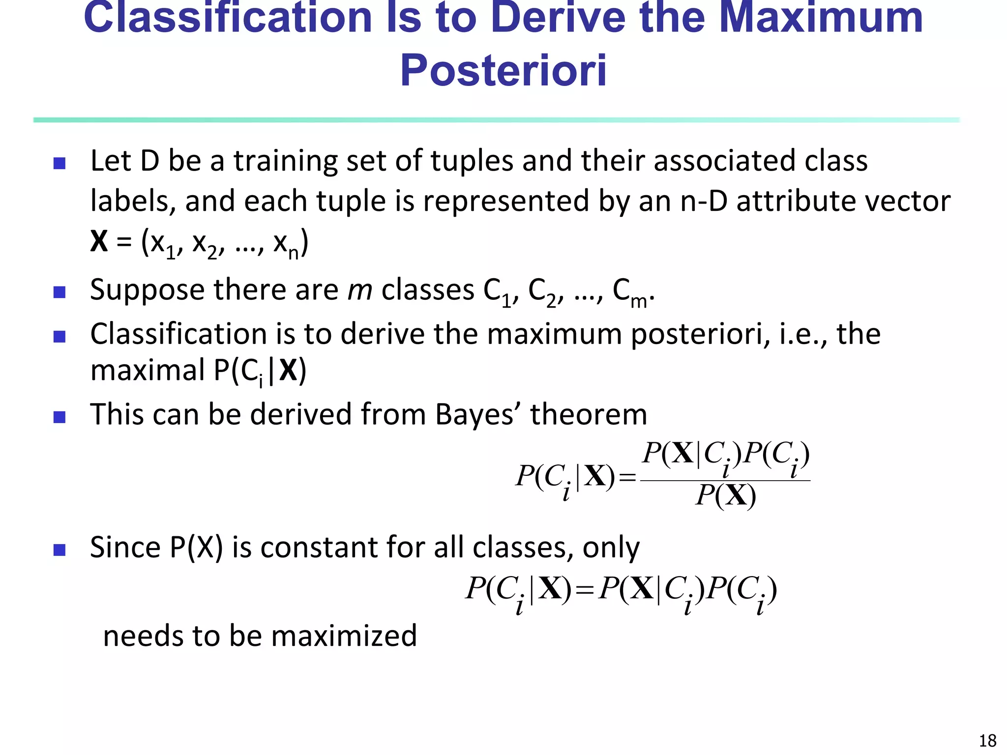
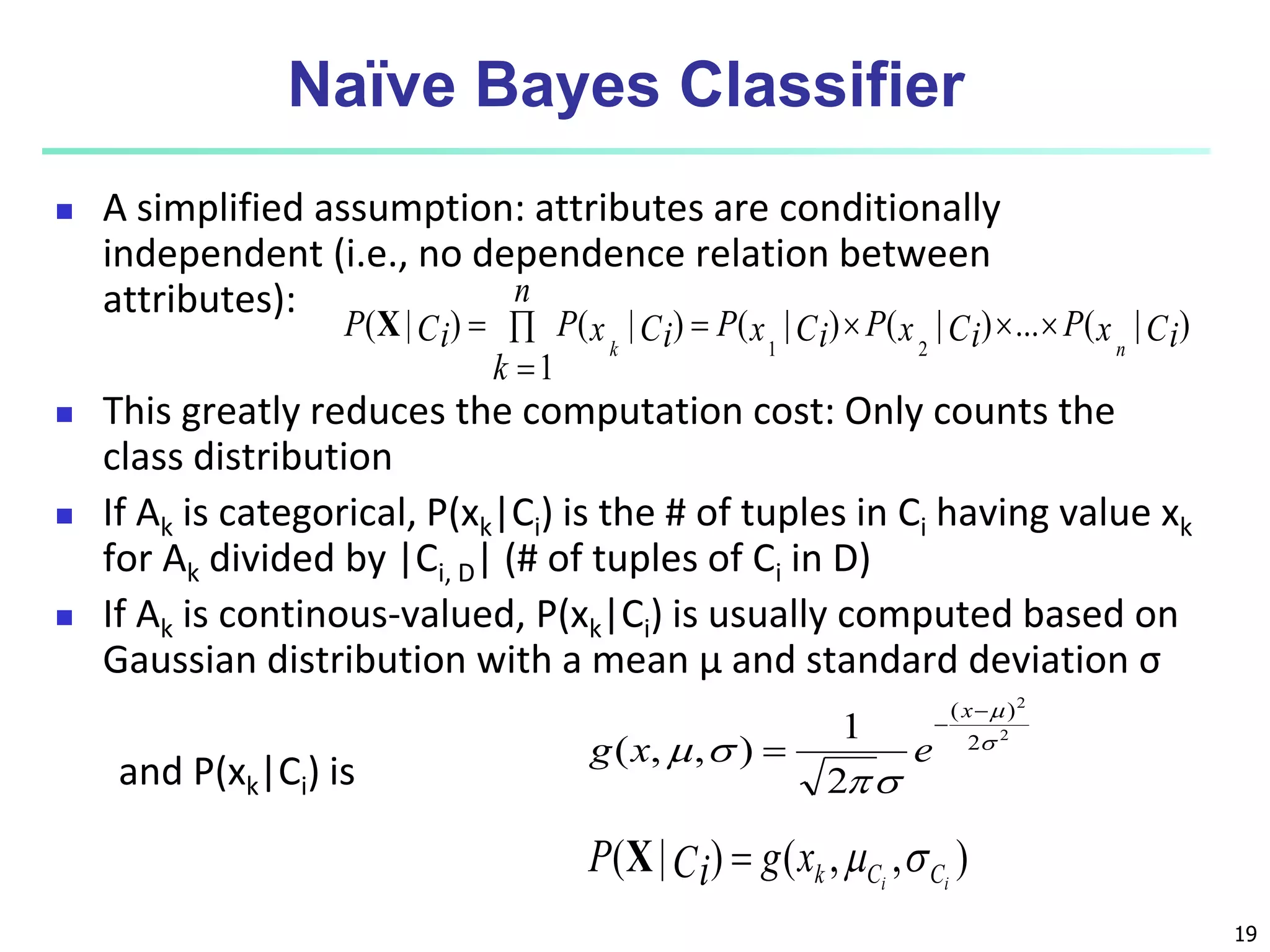
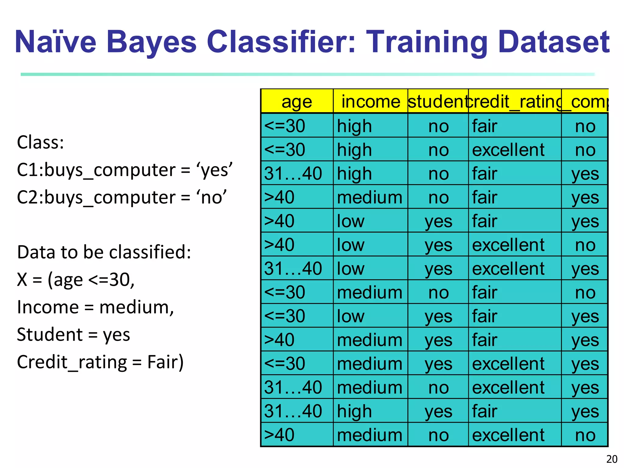
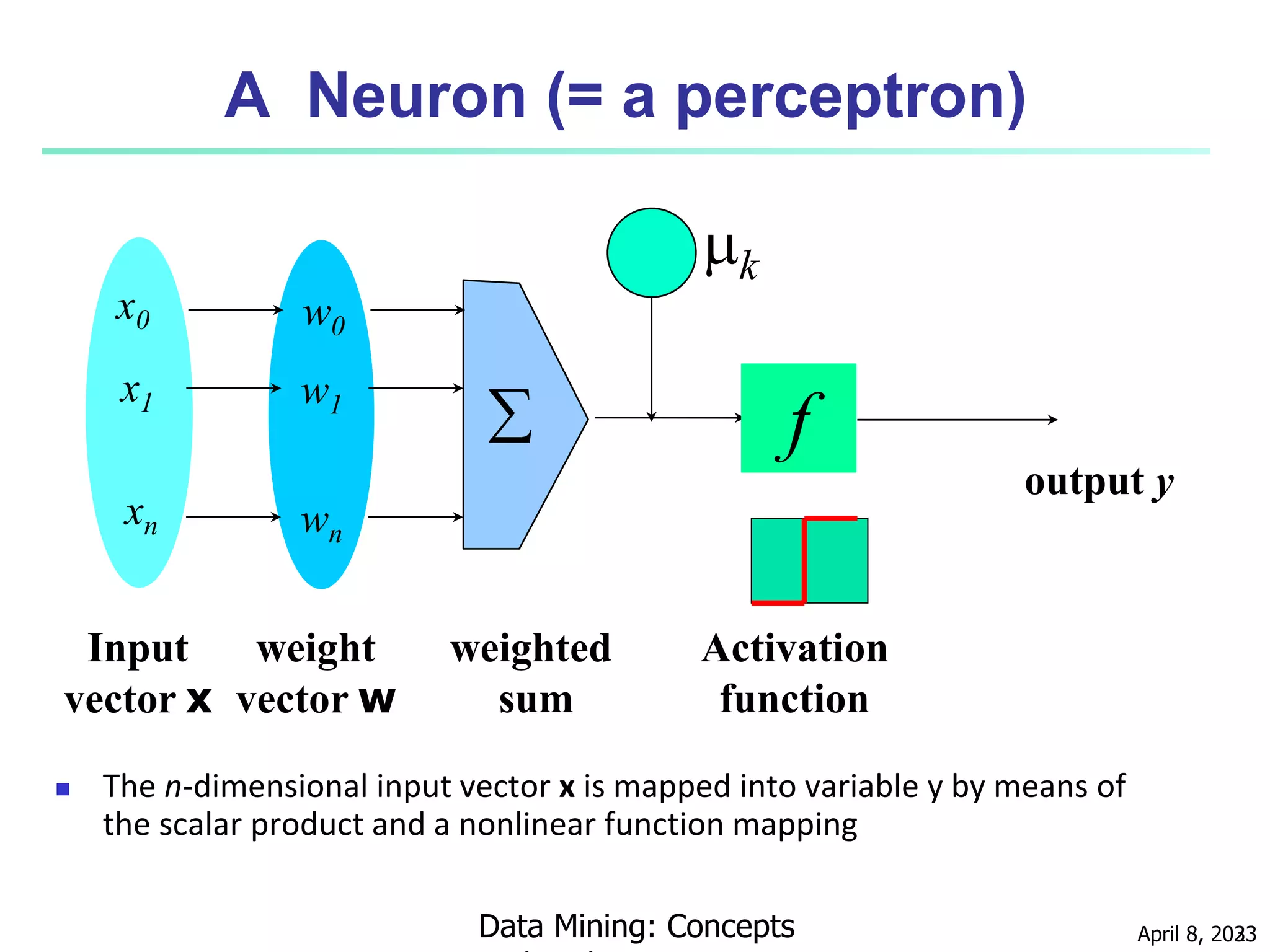
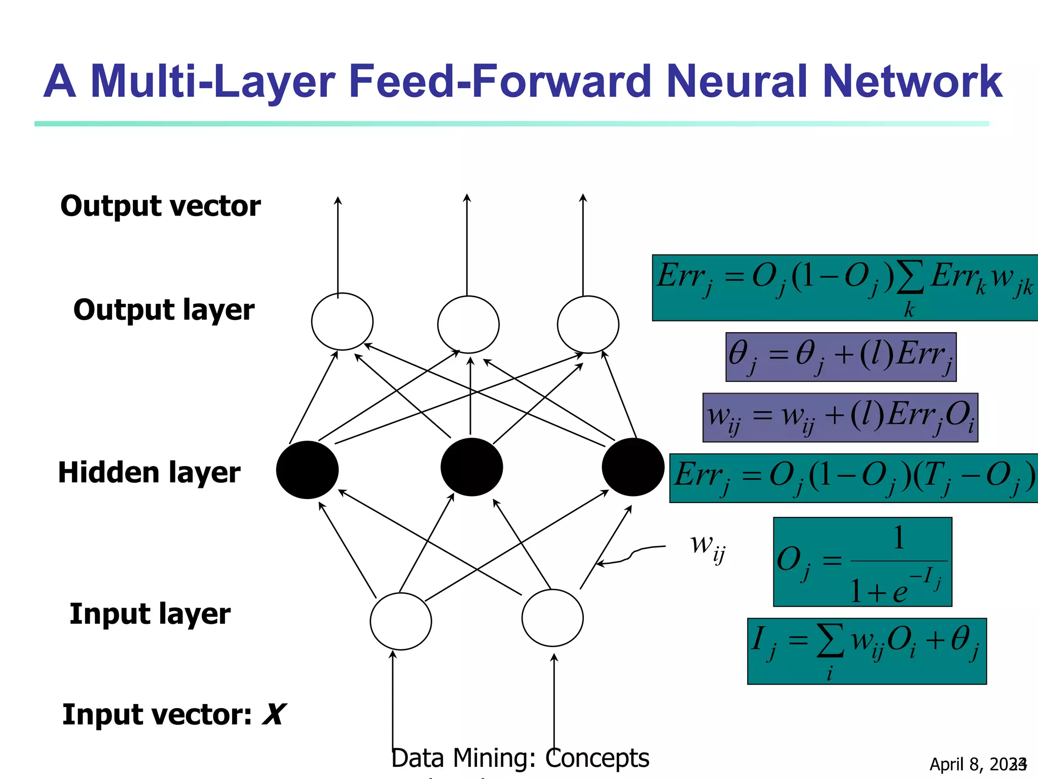
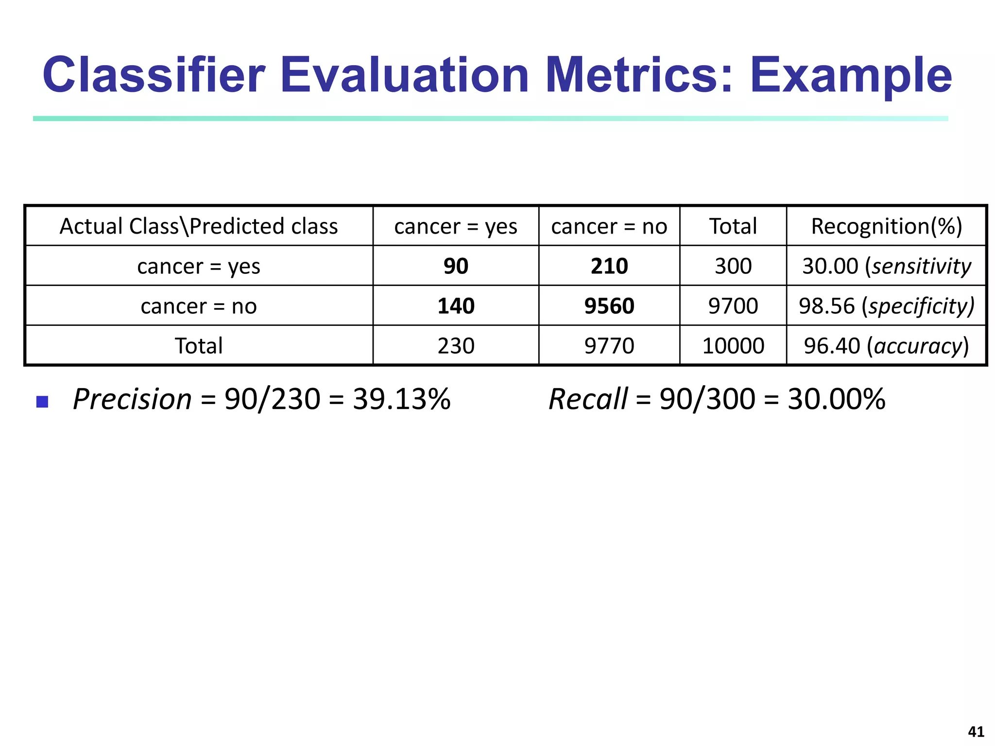
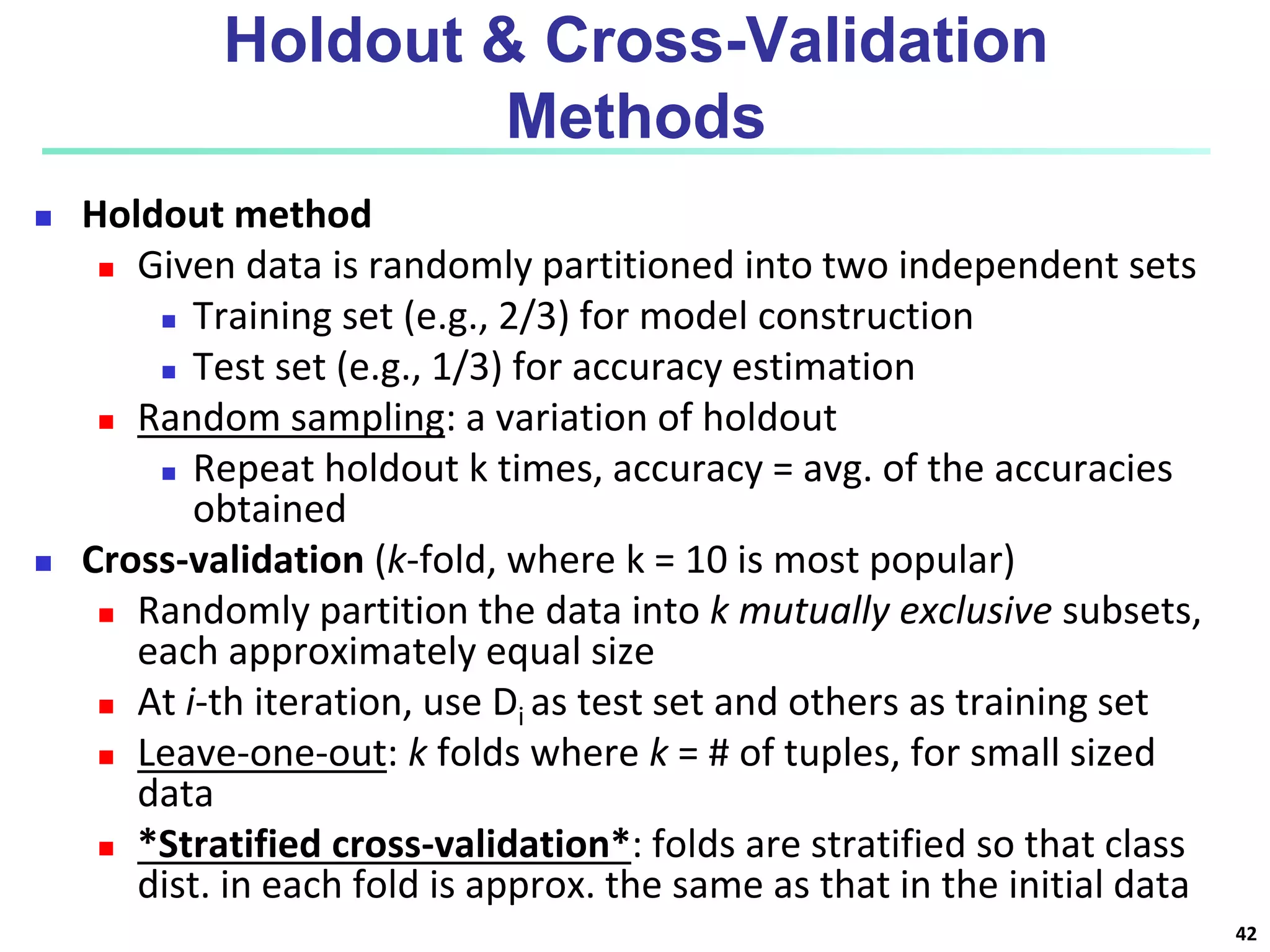
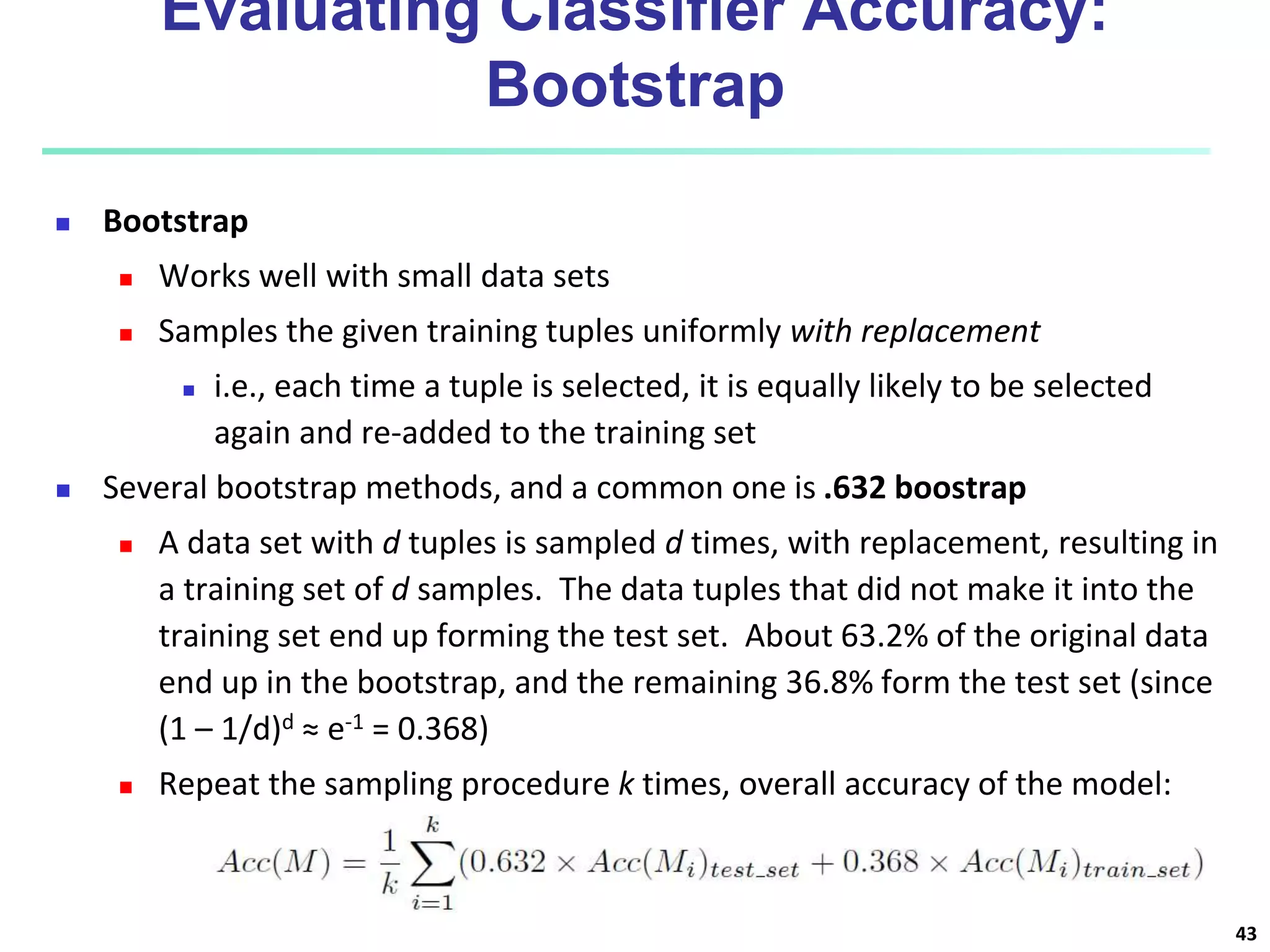
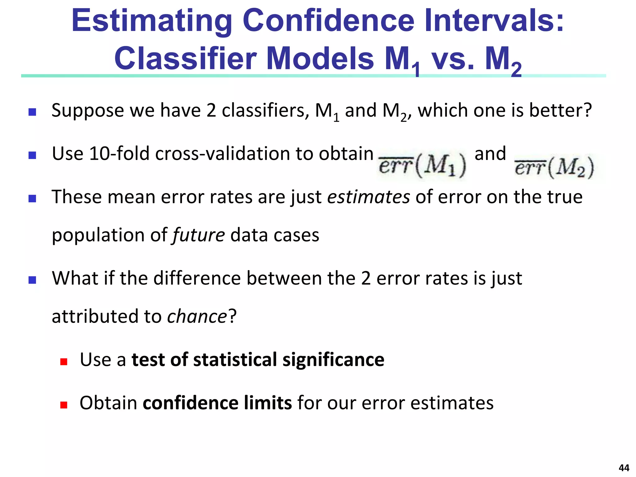
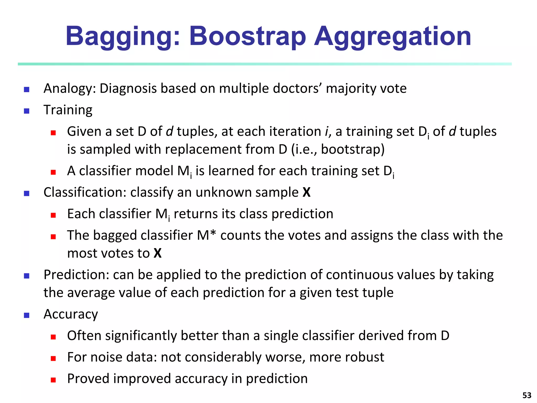
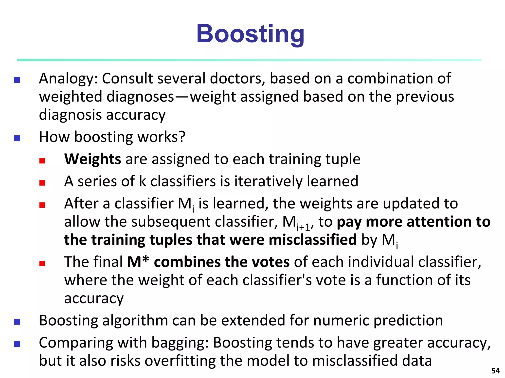
1
Unit: 4
Classification: Basic Concepts
 Classification: Basic Concepts
 Decision Tree Induction
 Bayes Classification Methods
 Rule-Based Classification
 Model Evaluation and Selection
 Techniques to Improve Classification Accuracy:
Ensemble Methods
 Summary

2
Supervised vs. Unsupervised Learning
 Supervised learning (classification)
 Supervision: The training data (observations,
measurements, etc.) are accompanied by labels indicating
the class of the observations
 New data is classified based on the training set
 Unsupervised learning (clustering)
 The class labels of training data is unknown
 Given a set of measurements, observations, etc. with the
aim of establishing the existence of classes or clusters in
the data

3
 Classification
 predicts categorical class labels (discrete or nominal)
 classifies data (constructs a model) based on the training
set and the values (class labels) in a classifying attribute
and uses it in classifying new data
 Numeric Prediction
 models continuous-valued functions, i.e., predicts
unknown or missing values
 Typical applications
 Credit/loan approval:
 Medical diagnosis
 Fraud detection: if a transaction is fraudulent
 Web page categorization: which category it is
Prediction Problems: Classification vs.
Numeric Prediction

4
Classification—A Two-Step
Process
 Model construction: describing a set of predetermined classes
 Each tuple/sample is assumed to belong to a predefined class, as
determined by the class label attribute
 The set of tuples used for model construction is training set
 The model is represented as classification rules, decision trees, or
mathematical formulae
 Model usage: for classifying future or unknown objects
 Estimate accuracy of the model
 The known label of test sample is compared with the classified
result from the model
 Accuracy rate is the percentage of test set samples that are
correctly classified by the model
 Test set is independent of training set (otherwise overfitting)
 If the accuracy is acceptable, use the model to classify new data
 Note: If the test set is used to select models, it is called validation (test) set

5
Process (1): Model Construction
Training
Data
NAME RANK YEARS TENURED
Mike Assistant Prof 3 no
Mary Assistant Prof 7 yes
Bill Professor 2 yes
Jim Associate Prof 7 yes
Dave Assistant Prof 6 no
Anne Associate Prof 3 no
Classification
Algorithms
IF rank = ‘professor’
OR years > 6
THEN tenured = ‘yes’
Classifier
(Model)

6
Process (2): Using the Model in
Prediction
Classifier
Testing
Data
NAME RANK YEARS TENURED
Tom Assistant Prof 2 no
Merlisa Associate Prof 7 no
George Professor 5 yes
Joseph Assistant Prof 7 yes
Unseen Data
(Jeff, Professor, 4)
Tenured?

7
Ensemble Methods
 Summary

8
Decision Tree Induction: An Example
age?
overcast
student? credit rating?
<=30 >40
no yes yes
yes
31..40
fair
excellent
yes
no
age income student credit_rating buys_computer
<=30 high no fair no
<=30 high no excellent no
31…40 high no fair yes
>40 medium no fair yes
>40 low yes fair yes
>40 low yes excellent no
31…40 low yes excellent yes
<=30 medium no fair no
<=30 low yes fair yes
>40 medium yes fair yes
<=30 medium yes excellent yes
31…40 medium no excellent yes
31…40 high yes fair yes
>40 medium no excellent no
 Training data set: Buys_computer
 Resulting tree:

9
Algorithm for Decision Tree Induction
 Basic algorithm (a greedy algorithm)
 Tree is constructed in a top-down recursive divide-and-
conquer manner
 At start, all the training examples are at the root
 Attributes are categorical (if continuous-valued, they are
discretized in advance)
 Examples are partitioned recursively based on selected
attributes
 Test attributes are selected on the basis of a heuristic or
statistical measure (e.g., information gain)
 Conditions for stopping partitioning
 All samples for a given node belong to the same class
 There are no remaining attributes for further partitioning –
majority voting is employed for classifying the leaf
 There are no samples left

10
Attribute Selection Measure:
Information Gain (ID3/C4.5)
 Select the attribute with the highest information gain
 Let pi be the probability that an arbitrary tuple in D belongs to
class Ci, estimated by |Ci, D|/|D|
 Expected information (entropy) needed to classify a tuple in D:
 Information needed (after using A to split D into v partitions) to
classify D:
 Information gained by branching on attribute A
)
(
log
)
( 2
1
i
m
i
i p
p
D
Info 



)
(
|
|
|
|
)
(
1
j
v
j
j
A D
Info
D
D
D
Info 
 

(D)
Info
Info(D)
Gain(A) A



11
Attribute Selection: Information Gain
 Class P: buys_computer = “yes”
 Class N: buys_computer = “no”
means “age <=30” has 5 out of
14 samples, with 2 yes’es and 3
no’s. Hence
Similarly,
age pi ni I(pi, ni)
<=30 2 3 0.971
31…40 4 0 0
>40 3 2 0.971
694
.
0
)
2
,
3
(
14
5
)
0
,
4
(
14
4
)
3
,
2
(
14
5
)
(




I
I
I
D
Infoage
048
.
0
)
_
(
151
.
0
)
(
029
.
0
)
(



rating
credit
Gain
student
Gain
income
Gain
246
.
0
)
(
)
(
)
( 

 D
Info
D
Info
age
Gain age
age income student credit_rating buys_computer
)
3
,
2
(
14
5
I
940
.
0
)
14
5
(
log
14
5
)
14
9
(
log
14
9
)
5
,
9
(
)
( 2
2 



 I
D
Info

12
Overfitting and Tree Pruning
 Overfitting: An induced tree may overfit the training data
 Too many branches, some may reflect anomalies due to
noise or outliers
 Poor accuracy for unseen samples
 Two approaches to avoid overfitting
 Prepruning: Halt tree construction early ̵ do not split a node
if this would result in the goodness measure falling below a
threshold
 Difficult to choose an appropriate threshold
 Postpruning: Remove branches from a “fully grown” tree—
get a sequence of progressively pruned trees
 Use a set of data different from the training data to
decide which is the “best pruned tree”

13
Enhancements to Basic Decision Tree
Induction
 Allow for continuous-valued attributes
 Dynamically define new discrete-valued attributes that
partition the continuous attribute value into a discrete set of
intervals
 Handle missing attribute values
 Assign the most common value of the attribute
 Assign probability to each of the possible values
 Attribute construction
 Create new attributes based on existing ones that are
sparsely represented
 This reduces fragmentation, repetition, and replication

14
Ensemble Methods
 Summary

15
Bayesian Classification: Why?
 A statistical classifier: performs probabilistic prediction, i.e.,
predicts class membership probabilities
 Foundation: Based on Bayes’ Theorem.
 Performance: A simple Bayesian classifier, naïve Bayesian
classifier, has comparable performance with decision tree and
selected neural network classifiers
 Incremental: Each training example can incrementally
increase/decrease the probability that a hypothesis is correct —
prior knowledge can be combined with observed data
 Standard: Even when Bayesian methods are computationally
intractable, they can provide a standard of optimal decision
making against which other methods can be measured

16
Bayes’ Theorem: Basics
 Total probability Theorem:
 Bayes’ Theorem:
 Let X be a data sample (“evidence”): class label is unknown
 Let H be a hypothesis that X belongs to class C
 Classification is to determine P(H|X), (i.e., posteriori probability): the
probability that the hypothesis holds given the observed data sample X
 P(H) (prior probability): the initial probability
 E.g., X will buy computer, regardless of age, income, …
 P(X): probability that sample data is observed
 P(X|H) (likelihood): the probability of observing the sample X, given that
the hypothesis holds
 E.g., Given that X will buy computer, the prob. that X is 31..40,
medium income
)
(
)
1
|
(
)
(
i
A
P
M
i i
A
B
P
B
P 


)
(
/
)
(
)
|
(
)
(
)
(
)
|
(
)
|
( X
X
X
X
X P
H
P
H
P
P
H
P
H
P
H
P 



17
Prediction Based on Bayes’ Theorem
 Given training data X, posteriori probability of a hypothesis H,
P(H|X), follows the Bayes’ theorem
 Informally, this can be viewed as
posteriori = likelihood x prior/evidence
 Predicts X belongs to Ci iff the probability P(Ci|X) is the highest
among all the P(Ck|X) for all the k classes
 Practical difficulty: It requires initial knowledge of many
probabilities, involving significant computational cost
)
(
/
)
(
)
|
(
)
(
)
(
)
|
(
)
|
( X
X
X
X
X P
H
P
H
P
P
H
P
H
P
H
P 



18
Classification Is to Derive the Maximum
Posteriori
 Let D be a training set of tuples and their associated class
labels, and each tuple is represented by an n-D attribute vector
X = (x1, x2, …, xn)
 Suppose there are m classes C1, C2, …, Cm.
 Classification is to derive the maximum posteriori, i.e., the
maximal P(Ci|X)
 This can be derived from Bayes’ theorem
 Since P(X) is constant for all classes, only
needs to be maximized
)
(
)
(
)
|
(
)
|
(
X
X
X
P
i
C
P
i
C
P
i
C
P 
)
(
)
|
(
)
|
(
i
C
P
i
C
P
i
C
P X
X 

19
Naïve Bayes Classifier
 A simplified assumption: attributes are conditionally
independent (i.e., no dependence relation between
attributes):
 This greatly reduces the computation cost: Only counts the
class distribution
 If Ak is categorical, P(xk|Ci) is the # of tuples in Ci having value xk
for Ak divided by |Ci, D| (# of tuples of Ci in D)
 If Ak is continous-valued, P(xk|Ci) is usually computed based on
Gaussian distribution with a mean μ and standard deviation σ
and P(xk|Ci) is
)
|
(
...
)
|
(
)
|
(
1
)
|
(
)
|
(
2
1
Ci
x
P
Ci
x
P
Ci
x
P
n
k
Ci
x
P
Ci
P
n
k







X
2
2
2
)
(
2
1
)
,
,
( 








x
e
x
g
)
,
,
(
)
|
( i
i C
C
k
x
g
Ci
P 


X

20
Naïve Bayes Classifier: Training Dataset
Class:
C1:buys_computer = ‘yes’
C2:buys_computer = ‘no’
Data to be classified:
X = (age <=30,
Income = medium,
Student = yes
Credit_rating = Fair)
age income student
credit_rating
buys_compu

21
Naïve Bayes Classifier: An Example
 P(Ci): P(buys_computer = “yes”) = 9/14 = 0.643
P(buys_computer = “no”) = 5/14= 0.357
 Compute P(X|Ci) for each class
P(age = “<=30” | buys_computer = “yes”) = 2/9 = 0.222
P(age = “<= 30” | buys_computer = “no”) = 3/5 = 0.6
P(income = “medium” | buys_computer = “yes”) = 4/9 = 0.444
P(income = “medium” | buys_computer = “no”) = 2/5 = 0.4
P(student = “yes” | buys_computer = “yes) = 6/9 = 0.667
P(student = “yes” | buys_computer = “no”) = 1/5 = 0.2
P(credit_rating = “fair” | buys_computer = “yes”) = 6/9 = 0.667
P(credit_rating = “fair” | buys_computer = “no”) = 2/5 = 0.4
 X = (age <= 30 , income = medium, student = yes, credit_rating = fair)
P(X|Ci) : P(X|buys_computer = “yes”) = 0.222 x 0.444 x 0.667 x 0.667 = 0.044
P(X|buys_computer = “no”) = 0.6 x 0.4 x 0.2 x 0.4 = 0.019
P(X|Ci)*P(Ci) : P(X|buys_computer = “yes”) * P(buys_computer = “yes”) = 0.028
P(X|buys_computer = “no”) * P(buys_computer = “no”) = 0.007
Therefore, X belongs to class (“buys_computer = yes”)
age income student
credit_rating
buys_comp

22
Naïve Bayes Classifier: Comments
 Advantages
 Easy to implement
 Good results obtained in most of the cases
 Disadvantages
 Assumption: class conditional independence, therefore loss
of accuracy
 Practically, dependencies exist among variables
 E.g., hospitals: patients: Profile: age, family history, etc.
Symptoms: fever, cough etc., Disease: lung cancer,
diabetes, etc.
 Dependencies among these cannot be modeled by Naïve
Bayes Classifier
 How to deal with these dependencies? Bayesian Belief Networks
(Chapter 9)

23
Ensemble Methods
 Summary

24
Using IF-THEN Rules for Classification
 Represent the knowledge in the form of IF-THEN rules
R: IF age = youth AND student = yes THEN buys_computer = yes
 Rule antecedent/precondition vs. rule consequent
 Assessment of a rule: coverage and accuracy
 ncovers = # of tuples covered by R
 ncorrect = # of tuples correctly classified by R
coverage(R) = ncovers /|D| /* D: training data set */
accuracy(R) = ncorrect / ncovers
 If more than one rule are triggered, need conflict resolution
 Size ordering: assign the highest priority to the triggering rules that has
the “toughest” requirement (i.e., with the most attribute tests)
 Class-based ordering: decreasing order of prevalence or misclassification
cost per class
 Rule-based ordering (decision list): rules are organized into one long
priority list, according to some measure of rule quality or by experts

25
age?
student? credit rating?
<=30 >40
no yes yes
yes
31..40
fair
excellent
yes
no
 Example: Rule extraction from our buys_computer decision-tree
IF age = young AND student = no THEN buys_computer = no
IF age = young AND student = yes THEN buys_computer = yes
IF age = mid-age THEN buys_computer = yes
IF age = old AND credit_rating = excellent THEN buys_computer = no
IF age = old AND credit_rating = fair THEN buys_computer = yes
Rule Extraction from a Decision Tree
 Rules are easier to understand than large
trees
 One rule is created for each path from the
root to a leaf
 Each attribute-value pair along a path forms a
conjunction: the leaf holds the class
prediction
 Rules are mutually exclusive and exhaustive

26
Rule Induction: Sequential Covering
Method
 Sequential covering algorithm: Extracts rules directly from training
data
 Typical sequential covering algorithms: FOIL, AQ, CN2, RIPPER
 Rules are learned sequentially, each for a given class Ci will cover
many tuples of Ci but none (or few) of the tuples of other classes
 Steps:
 Rules are learned one at a time
 Each time a rule is learned, the tuples covered by the rules are
removed
 Repeat the process on the remaining tuples until termination
condition, e.g., when no more training examples or when the
quality of a rule returned is below a user-specified threshold
 Comp. w. decision-tree induction: learning a set of rules
simultaneously

27
Sequential Covering Algorithm
while (enough target tuples left)
generate a rule
remove positive target tuples satisfying this rule
Examples covered
by Rule 3
Examples covered
by Rule 2
Examples covered
by Rule 1
Positive
examples

28
Rule Generation
 To generate a rule
while(true)
find the best predicate p
if foil-gain(p) > threshold then add p to current rule
else break
Positive
examples
Negative
examples
A3=1
A3=1&&A1=2
A3=1&&A1=2
&&A8=5

29
How to Learn-One-Rule?
 Start with the most general rule possible: condition = empty
 Adding new attributes by adopting a greedy depth-first strategy
 Picks the one that most improves the rule quality
 Rule-Quality measures: consider both coverage and accuracy
 Foil-gain (in FOIL & RIPPER): assesses info_gain by extending
condition
 favors rules that have high accuracy and cover many positive tuples
 Rule pruning based on an independent set of test tuples
Pos/neg are # of positive/negative tuples covered by R.
If FOIL_Prune is higher for the pruned version of R, prune R
)
log
'
'
'
(log
'
_ 2
2
neg
pos
pos
neg
pos
pos
pos
Gain
FOIL





neg
pos
neg
pos
R
Prune
FOIL



)
(
_

30
 Classification by Neural networks
Ensemble Methods

April 8, 2023
31
Classification by Neural Networks (Backpropagation)
 Backpropagation: A neural network learning algorithm
 A neural network: A set of connected input/output units
where each connection has a weight associated with it
 During the learning phase, the network learns by adjusting
the weights so as to be able to predict the correct class label
of the input tuples
 Also referred to as connectionist learning due to the
connections between units

April 8, 2023
Data Mining: Concepts 32
Neural Network as a Classifier
 Weakness
 Long training time
 Poor interpretability: Difficult to interpret the
symbolic meaning behind the learned weights and
of “hidden units" in the network
 Strength
 High tolerance to noisy data
 Ability to classify untrained patterns
 Well-suited for continuous-valued inputs and
outputs

April 8, 2023
A Neuron (= a perceptron)
 The n-dimensional input vector x is mapped into variable y by means of
the scalar product and a nonlinear function mapping
k
-
f
weighted
sum
Input
vector x
output y
Activation
function
weight
vector w

w0
w1
wn
x0
x1
xn

April 8, 2023
A Multi-Layer Feed-Forward Neural Network
Output layer
Input layer
Hidden layer
Output vector
Input vector: X
wij
 

i
j
i
ij
j O
w
I 
j
I
j
e
O 


1
1
)
)(
1
( j
j
j
j
j O
T
O
O
Err 


jk
k
k
j
j
j w
Err
O
O
Err 

 )
1
(
i
j
ij
ij O
Err
l
w
w )
(


j
j
j Err
l)
(




April 8, 2023
How A Multi-Layer Neural Network Works?
 The inputs to the network correspond to the attributes measured for each
training tuple
 Inputs are fed simultaneously into the units making up the input layer
 They are then weighted and fed simultaneously to a hidden layer
 The number of hidden layers is arbitrary, although usually only one
 The weighted outputs of the last hidden layer are input to units making up
the output layer, which emits the network's prediction
 The network is feed-forward in that none of the weights cycles back to an
input unit or to an output unit of a previous layer

April 8, 2023
Backpropagation
 Iteratively process a set of training tuples & compare the network's
prediction with the actual known target value
 For each training tuple, the weights are modified to minimize the mean
squared error between the network's prediction and the actual target value
 Modifications are made in the “backwards” direction: from the output layer,
through each hidden layer down to the first hidden layer, hence
“backpropagation”
 Steps
 Initialize weights (to small random #s) and biases in the network
 Propagate the inputs forward (by applying activation function)
 Backpropagate the error (by updating weights and biases)
 Terminating condition (when error is very small, etc.)

Model Evaluation and Selection
 Evaluation metrics: How can we measure accuracy? Other
metrics to consider?
 Use validation test set of class-labeled tuples instead of
training set when assessing accuracy
 Methods for estimating a classifier’s accuracy:
 Holdout method, random subsampling
 Cross-validation
 Bootstrap
 Comparing classifiers:
 Confidence intervals
 Cost-benefit analysis and ROC Curves
37

Classifier Evaluation Metrics: Confusion
Matrix
Actual classPredicted
class
buy_computer
= yes
buy_computer
= no
Total
buy_computer = yes 6954 46 7000
buy_computer = no 412 2588 3000
Total 7366 2634 10000
 Given m classes, an entry, CMi,j in a confusion matrix indicates
# of tuples in class i that were labeled by the classifier as class j
 May have extra rows/columns to provide totals
Confusion Matrix:
Actual classPredicted class C1 ¬ C1
C1 True Positives (TP) False Negatives (FN)
¬ C1 False Positives (FP) True Negatives (TN)
Example of Confusion Matrix:
38

Accuracy, Error Rate, Sensitivity and
Specificity
 Classifier Accuracy, or
recognition rate: percentage of
test set tuples that are correctly
classified
Accuracy = (TP + TN)/All
 Error rate: 1 – accuracy, or
Error rate = (FP + FN)/All
 Class Imbalance Problem:
 One class may be rare, e.g.
fraud, or HIV-positive
 Significant majority of the
negative class and minority of
the positive class
 Sensitivity: True Positive
recognition rate
 Sensitivity = TP/P
 Specificity: True Negative
recognition rate
 Specificity = TN/N
AP C ¬C
C TP FN P
¬C FP TN N
P’ N’ All
39

Precision and Recall, and F-
measures
 Precision: exactness – what % of tuples that the classifier
labeled as positive are actually positive
 Recall: completeness – what % of positive tuples did the
classifier label as positive?
 Perfect score is 1.0
 Inverse relationship between precision & recall
 F measure (F1 or F-score): harmonic mean of precision and
recall,
 Fß: weighted measure of precision and recall
 assigns ß times as much weight to recall as to precision
40

Classifier Evaluation Metrics: Example
41
 Precision = 90/230 = 39.13% Recall = 90/300 = 30.00%
Actual ClassPredicted class cancer = yes cancer = no Total Recognition(%)
cancer = yes 90 210 300 30.00 (sensitivity
cancer = no 140 9560 9700 98.56 (specificity)
Total 230 9770 10000 96.40 (accuracy)

Holdout & Cross-Validation
Methods
 Holdout method
 Given data is randomly partitioned into two independent sets
 Training set (e.g., 2/3) for model construction
 Test set (e.g., 1/3) for accuracy estimation
 Random sampling: a variation of holdout
 Repeat holdout k times, accuracy = avg. of the accuracies
obtained
 Cross-validation (k-fold, where k = 10 is most popular)
 Randomly partition the data into k mutually exclusive subsets,
each approximately equal size
 At i-th iteration, use Di as test set and others as training set
 Leave-one-out: k folds where k = # of tuples, for small sized
data
 *Stratified cross-validation*: folds are stratified so that class
dist. in each fold is approx. the same as that in the initial data
42

Evaluating Classifier Accuracy:
Bootstrap
 Bootstrap
 Works well with small data sets
 Samples the given training tuples uniformly with replacement
 i.e., each time a tuple is selected, it is equally likely to be selected
again and re-added to the training set
 Several bootstrap methods, and a common one is .632 boostrap
 A data set with d tuples is sampled d times, with replacement, resulting in
a training set of d samples. The data tuples that did not make it into the
training set end up forming the test set. About 63.2% of the original data
end up in the bootstrap, and the remaining 36.8% form the test set (since
(1 – 1/d)d ≈ e-1 = 0.368)
 Repeat the sampling procedure k times, overall accuracy of the model:
43

Estimating Confidence Intervals:
Classifier Models M1 vs. M2
 Suppose we have 2 classifiers, M1 and M2, which one is better?
 Use 10-fold cross-validation to obtain and
 These mean error rates are just estimates of error on the true
population of future data cases
 What if the difference between the 2 error rates is just
attributed to chance?
 Use a test of statistical significance
 Obtain confidence limits for our error estimates
44

Null Hypothesis
 Perform 10-fold cross-validation
 Assume samples follow a t distribution with k–1 degrees of
freedom (here, k=10)
 Use t-test (or Student’s t-test)
 Null Hypothesis: M1 & M2 are the same
 If we can reject null hypothesis, then
 we conclude that the difference between M1 & M2 is
statistically significant
 Chose model with lower error rate
45

Estimating Confidence Intervals: t-test
 If only 1 test set available: pairwise comparison
 For ith round of 10-fold cross-validation, the same cross
partitioning is used to obtain err(M1)i and err(M2)i
 Average over 10 rounds to get
 t-test computes t-statistic with k-1 degrees of
freedom:
 If two test sets available: use non-paired t-test
where
and
where
where k1 & k2 are # of cross-validation samples used for M1 & M2, resp.
46

Table for t-distribution
 Symmetric
 Significance level,
e.g., sig = 0.05 or
5% means M1 & M2
are significantly
different for 95% of
population
 Confidence limit, z
= sig/2
47

Statistical Significance
 Are M1 & M2 significantly different?
 Compute t. Select significance level (e.g. sig = 5%)
 Consult table for t-distribution: Find t value corresponding
to k-1 degrees of freedom (here, 9)
 t-distribution is symmetric: typically upper % points of
distribution shown → look up value for confidence limit
z=sig/2 (here, 0.025)
 If t > z or t < -z, then t value lies in rejection region:
 Reject null hypothesis that mean error rates of M1 & M2
are same
 Conclude: statistically significant difference between M1
& M2
 Otherwise, conclude that any difference is chance
48

Model Selection: ROC Curves
 ROC (Receiver Operating
Characteristics) curves: for visual
comparison of classification models
 Originated from signal detection theory
 Shows the trade-off between the true
positive rate and the false positive rate
 The area under the ROC curve is a
measure of the accuracy of the model
 Rank the test tuples in decreasing
order: the one that is most likely to
belong to the positive class appears at
the top of the list
 The closer to the diagonal line (i.e., the
closer the area is to 0.5), the less
accurate is the model
 Vertical axis
represents the true
positive rate
 Horizontal axis rep.
the false positive rate
 The plot also shows a
diagonal line
 A model with perfect
accuracy will have an
area of 1.0
49

Issues Affecting Model Selection
 Accuracy
 classifier accuracy: predicting class label
 Speed
 time to construct the model (training time)
 time to use the model (classification/prediction time)
 Robustness: handling noise and missing values
 Scalability: efficiency in disk-resident databases
 Interpretability
 understanding and insight provided by the model
 Other measures, e.g., goodness of rules, such as decision tree
size or compactness of classification rules
50

51
Ensemble Methods
 Summary

Ensemble Methods: Increasing the
Accuracy
 Ensemble methods
 Use a combination of models to increase accuracy
 Combine a series of k learned models, M1, M2, …, Mk, with
the aim of creating an improved model M*
 Popular ensemble methods
 Bagging: averaging the prediction over a collection of
classifiers
 Boosting: weighted vote with a collection of classifiers
 Ensemble: combining a set of heterogeneous classifiers
52

Bagging: Boostrap Aggregation
 Analogy: Diagnosis based on multiple doctors’ majority vote
 Training
 Given a set D of d tuples, at each iteration i, a training set Di of d tuples
is sampled with replacement from D (i.e., bootstrap)
 A classifier model Mi is learned for each training set Di
 Classification: classify an unknown sample X
 Each classifier Mi returns its class prediction
 The bagged classifier M* counts the votes and assigns the class with the
most votes to X
 Prediction: can be applied to the prediction of continuous values by taking
the average value of each prediction for a given test tuple
 Accuracy
 Often significantly better than a single classifier derived from D
 For noise data: not considerably worse, more robust
 Proved improved accuracy in prediction
53

Boosting
 Analogy: Consult several doctors, based on a combination of
weighted diagnoses—weight assigned based on the previous
diagnosis accuracy
 How boosting works?
 Weights are assigned to each training tuple
 A series of k classifiers is iteratively learned
 After a classifier Mi is learned, the weights are updated to
allow the subsequent classifier, Mi+1, to pay more attention to
the training tuples that were misclassified by Mi
 The final M* combines the votes of each individual classifier,
where the weight of each classifier's vote is a function of its
accuracy
 Boosting algorithm can be extended for numeric prediction
 Comparing with bagging: Boosting tends to have greater accuracy,
but it also risks overfitting the model to misclassified data 54

Unit-4 classification

More Related Content

Similar to Unit-4 classification

Recently uploaded

Unit-4 classification