The document discusses the principles of classification in data mining and warehousing, focusing on supervised learning methods including decision trees, naive Bayesian classification, and ensemble methods. It outlines processes for model construction and usage, evaluates classification methods based on accuracy, and addresses issues of overfitting and underfitting in decision trees. It also highlights various attribute selection measures and their application in constructing effective classification models.
Overview of Sanjivani College of Engineering and the Data Mining unit focusing on classification methods.
Distinction between supervised (classification) and unsupervised (clustering) learning, focusing on prediction problems in classification.
Description of the two-step classification process involving model construction and its usage for classifying new data.
Challenges in data preparation including data cleaning, feature selection, and transformation necessary for effective classification.
Importance of accuracy in classifier evaluation, the use of confusion matrices for assessing prediction performance.
The process of decision tree induction, training datasets, algorithms, and greedy approach to partitioning.
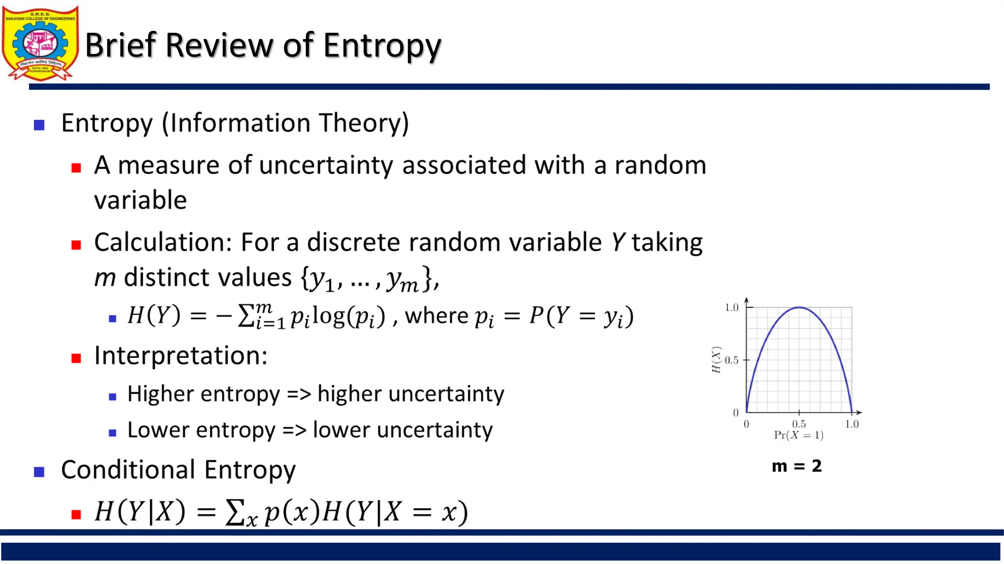
Understanding entropy, information gain for attribute selection in decision trees, and practical examples using datasets.
Methods for dealing with continuous attributes in decision trees, including Gini index for impurity reduction.
Analysis of various attribute selection measures and their strengths and weaknesses in decision tree algorithms.
Issues of overfitting and underfitting in decision trees and techniques like prepruning and postpruning to improve models.
Enhancements in decision trees for continuous attributes, handling missing values, and introducing new derived attributes.Introduction to Bayesian classification, foundations, and application of Bayes' theorem in predicting class memberships.
The Naïve Bayes classifier process, including the classification of new incoming data based on trained probabilities.
Evaluation metrics such as accuracy, precision, recall, and methods to compare classifier performance including confusion matrices.
Contrasts between lazy and eager learning, focusing on methods like instance-based learning vs model construction.
Steps and principles of the k-nearest neighbors algorithm, including distance calculations for classification.
Introduction to regression as a prediction method, linear regression models, and their representation.
Description of ensemble methods in classification, highlighting techniques like bagging and boosting for improving model accuracy.
Sanjivani Rural EducationSociety’s
Sanjivani College of Engineering, Kopargaon-423 603
(An Autonomous Institute, Affiliated to Savitribai Phule Pune University, Pune)
NACC ‘A’ Grade Accredited, ISO 9001:2015 Certified
Department of Computer Engineering
(NBA Accredited)
Prof. S. A. Shivarkar
Assistant Professor
Contact No.8275032712
Email- shivarkarsandipcomp@sanjivani.org.in
Subject- Data Mining and Warehousing (CO314)
Unit –VI: Classification
2.
Content
Introduction, classificationrequirements, methods of supervised learning
Decision trees- attribute selection measures (info gain, Gini ratio, Gini
index), scalable decision tree techniques, rule extraction from decision tree,
Naïve bayesian Classification, Rule based classification
Associative Classification, Lazy Learners-k-Nearest- Multiclass Classification,
Metrics for Evaluating Classifier Evaluating the Accuracy of a Classifier
Regression, Introduction to Ensemble Methods.
3.
Supervised vs. UnsupervisedLearning
Supervised learning (classification)
Supervision: The training data (observations, measurements, etc.) are
accompanied by labels indicating the class of the observations
New data is classified based on the training set
Unsupervised learning (clustering)
The class labels of training data is unknown
Given a set of measurements, observations, etc. with the aim of
establishing the existence of classes or clusters in the data
4.
Prediction Problems: Classificationvs. Numeric Prediction
Classification
predicts categorical class labels (discrete or nominal)
classifies data (constructs a model) based on the training set and the
values (class labels) in a classifying attribute and uses it in classifying new
data
Numeric Prediction
models continuous-valued functions, i.e., predicts unknown or missing
values
Typical applications
Credit/loan approval:
Medical diagnosis: if a tumor is cancerous or benign
Fraud detection: if a transaction is fraudulent
Web page categorization: which category it is
5.
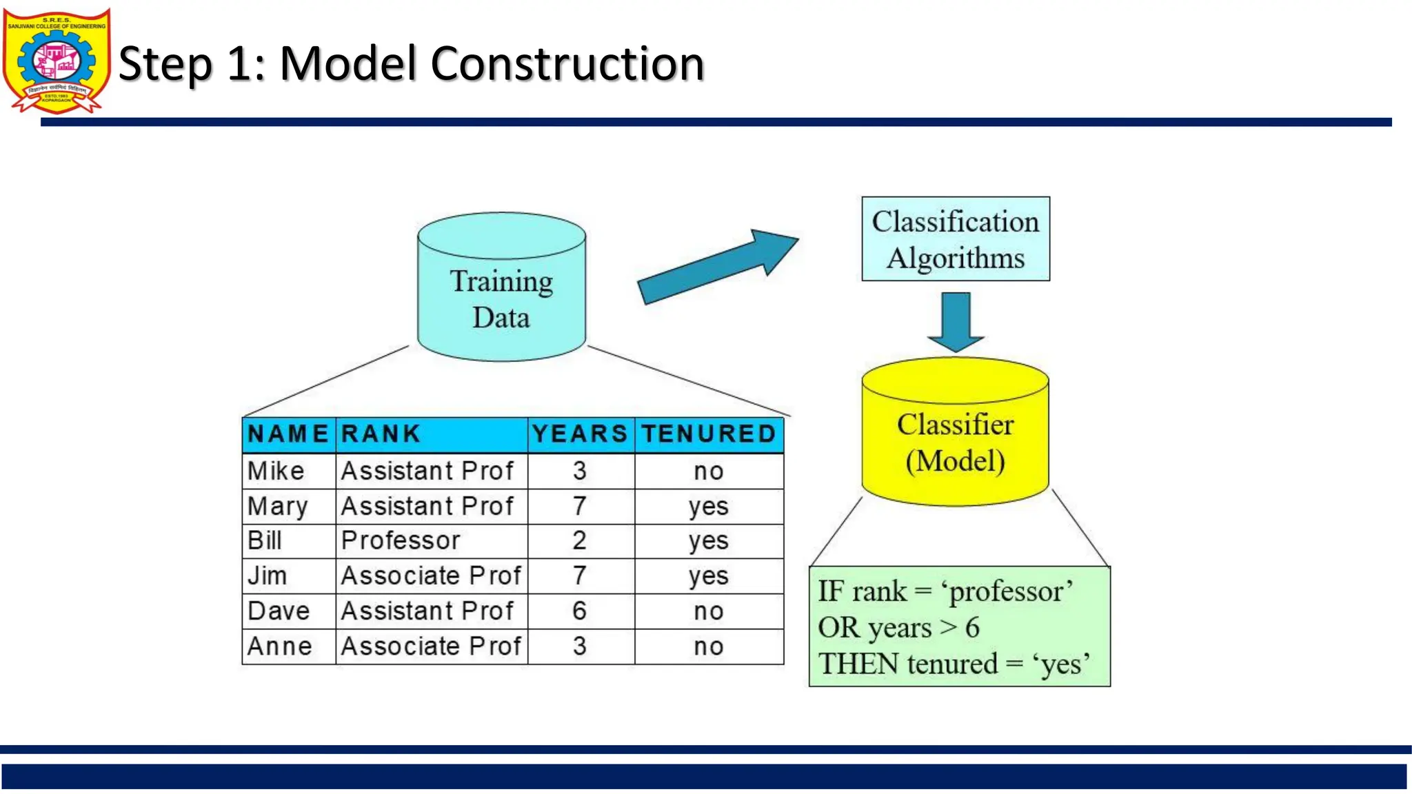
Classification—A Two-Step Process
Model construction: describing a set of predetermined classes
Each tuple/sample is assumed to belong to a predefined class, as determined by the class
label attribute
The set of tuples used for model construction is training set
The model is represented as classification rules, decision trees, or mathematical formulae
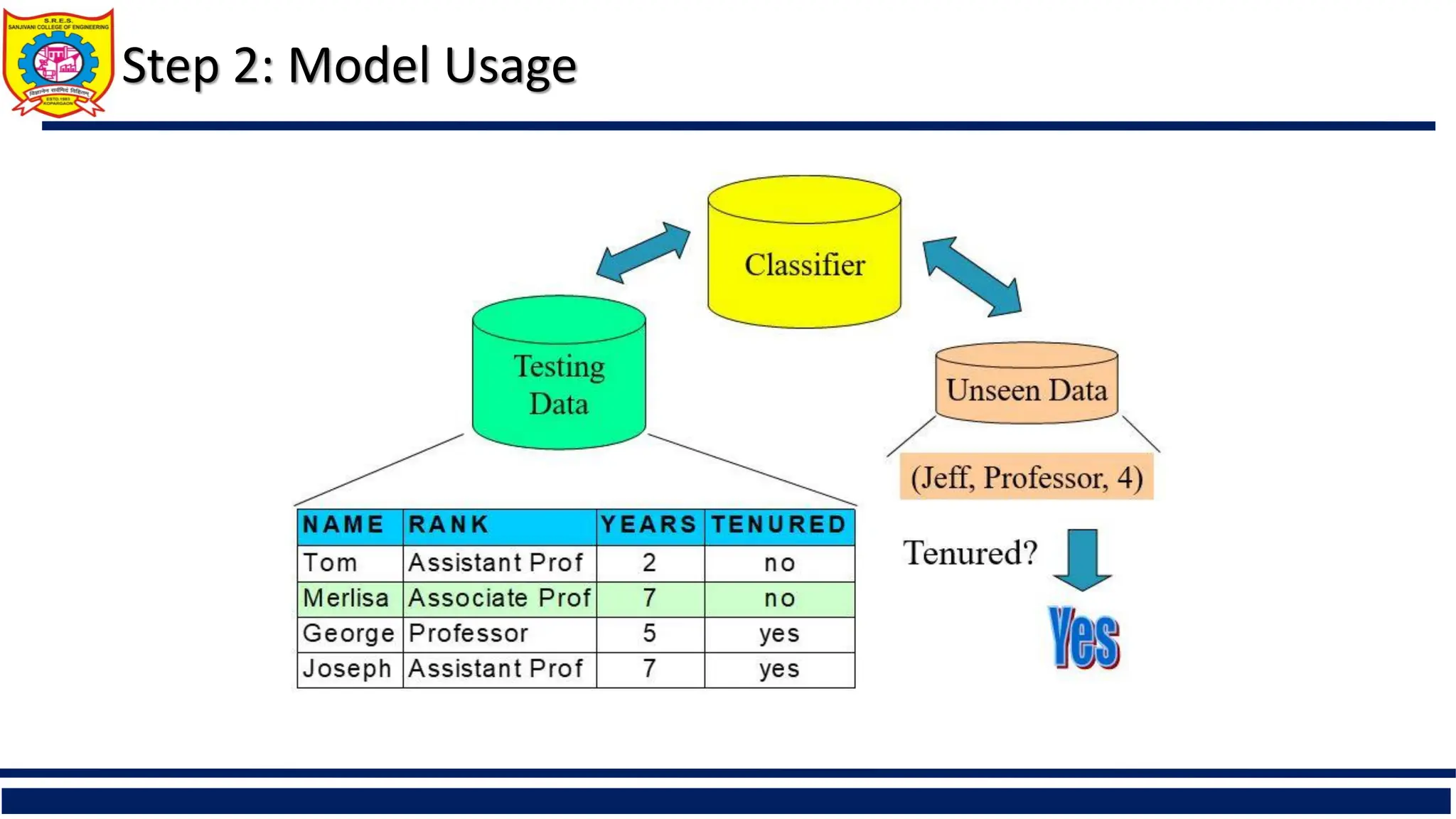
Model usage: for classifying future or unknown objects
Estimate accuracy of the model
The known label of test sample is compared with the classified result from the model
Accuracy rate is the percentage of test set samples that are correctly classified by the
model
Test set is independent of training set (otherwise overfitting)
If the accuracy is acceptable, use the model to classify new data
Note: If the test set is used to select models, it is called validation (test) set
Issues: Data Preparation
Data cleaning
Preprocess data in order to reduce noise and handle
missing values
Relevance analysis (feature selection)
Remove the irrelevant or redundant attributes
Data transformation
Generalize and/or normalize data
9.
Issues: Evaluating ClassificationMethods
Accuracy
classifier accuracy: predicting class label
predictor accuracy: guessing value of predicted attributes
Speed
time to construct the model (training time)
time to use the model (classification/prediction time)
Robustness: handling noise and missing values
Scalability: efficiency in disk-resident databases
Interpretability
understanding and insight provided by the model
Other measures, e.g., goodness of rules, such as decision tree size or compactness of classification rules
10.
Issues: Evaluating ClassificationMethods: Accuracy
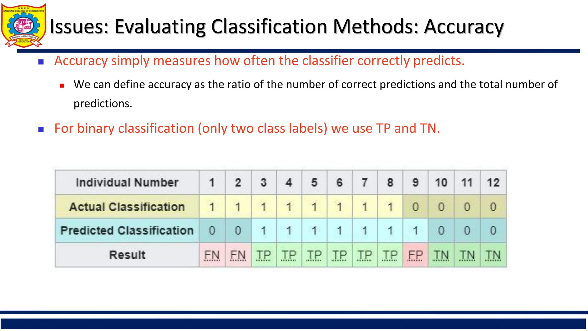
Accuracy simply measures how often the classifier correctly predicts.
We can define accuracy as the ratio of the number of correct predictions and the total number of
predictions.
For binary classification (only two class labels) we use TP and TN.
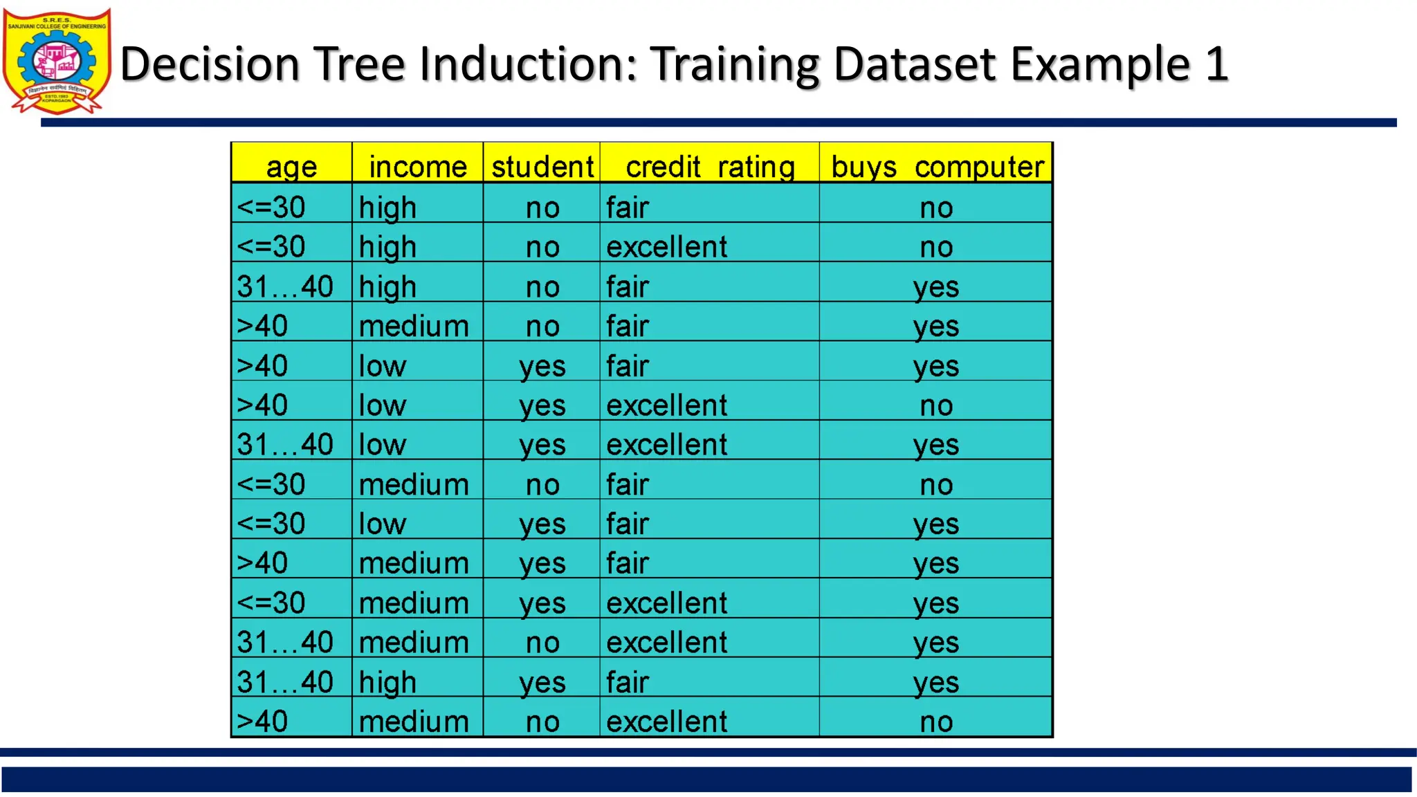
Decision Tree Induction:Training Dataset
age?
overcast
student? credit rating?
<=30 >40
no yes yes
yes
31..40
fair
excellent
yes
no
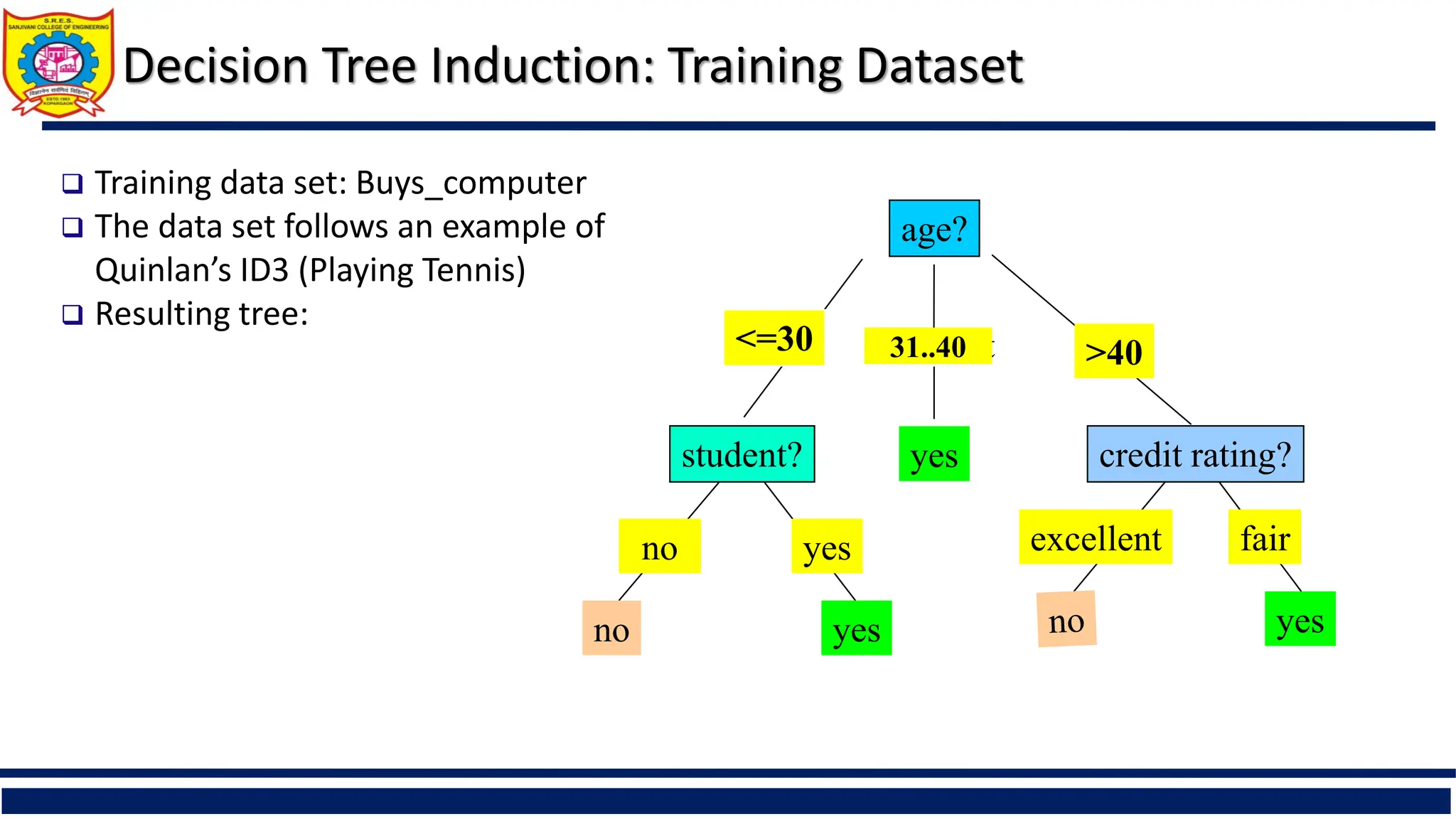
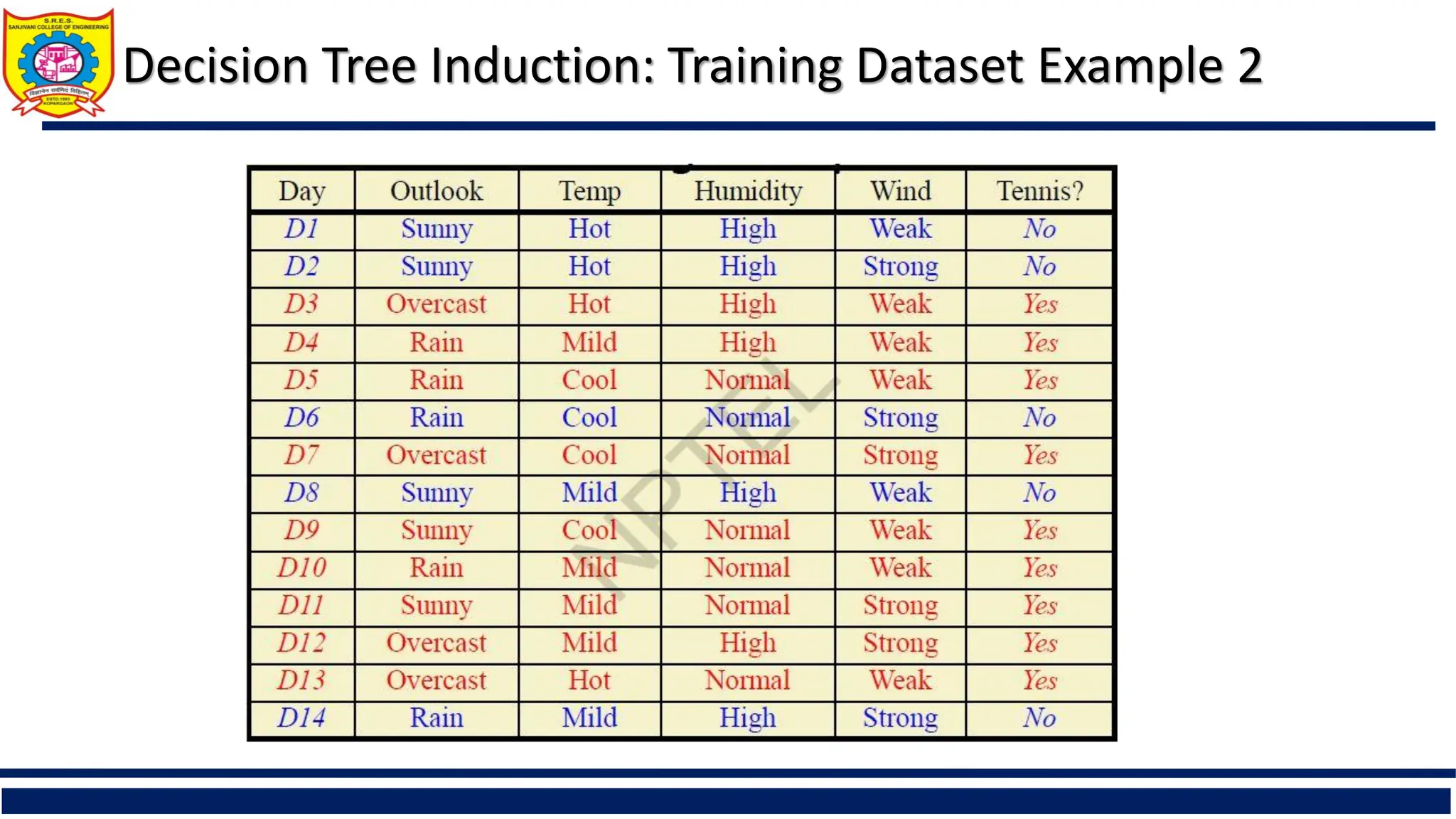
Training data set: Buys_computer
The data set follows an example of
Quinlan’s ID3 (Playing Tennis)
Resulting tree:
14.
Algorithm for DecisionTree Induction
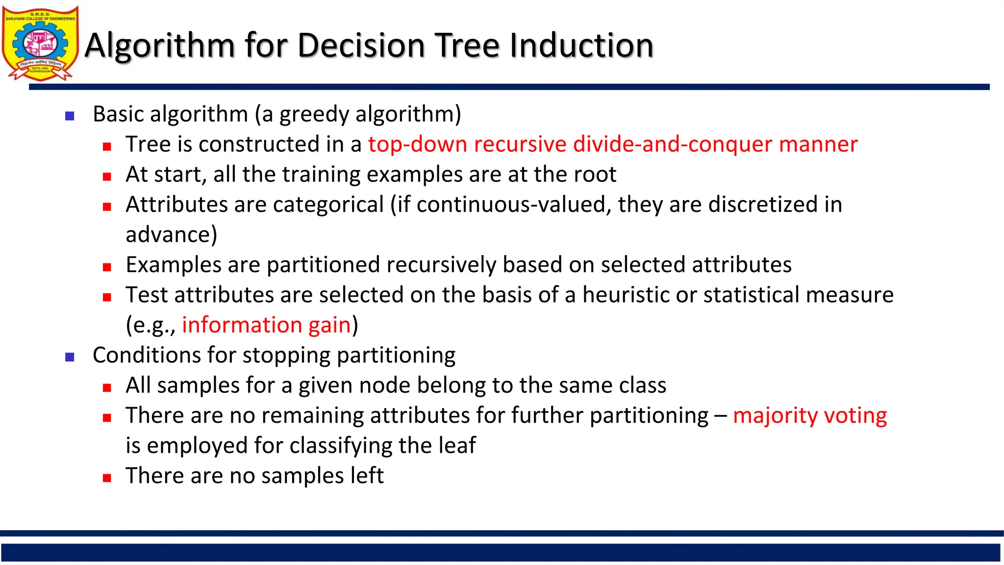
Basic algorithm (a greedy algorithm)
Tree is constructed in a top-down recursive divide-and-conquer manner
At start, all the training examples are at the root
Attributes are categorical (if continuous-valued, they are discretized in
advance)
Examples are partitioned recursively based on selected attributes
Test attributes are selected on the basis of a heuristic or statistical measure
(e.g., information gain)
Conditions for stopping partitioning
All samples for a given node belong to the same class
There are no remaining attributes for further partitioning – majority voting
is employed for classifying the leaf
There are no samples left
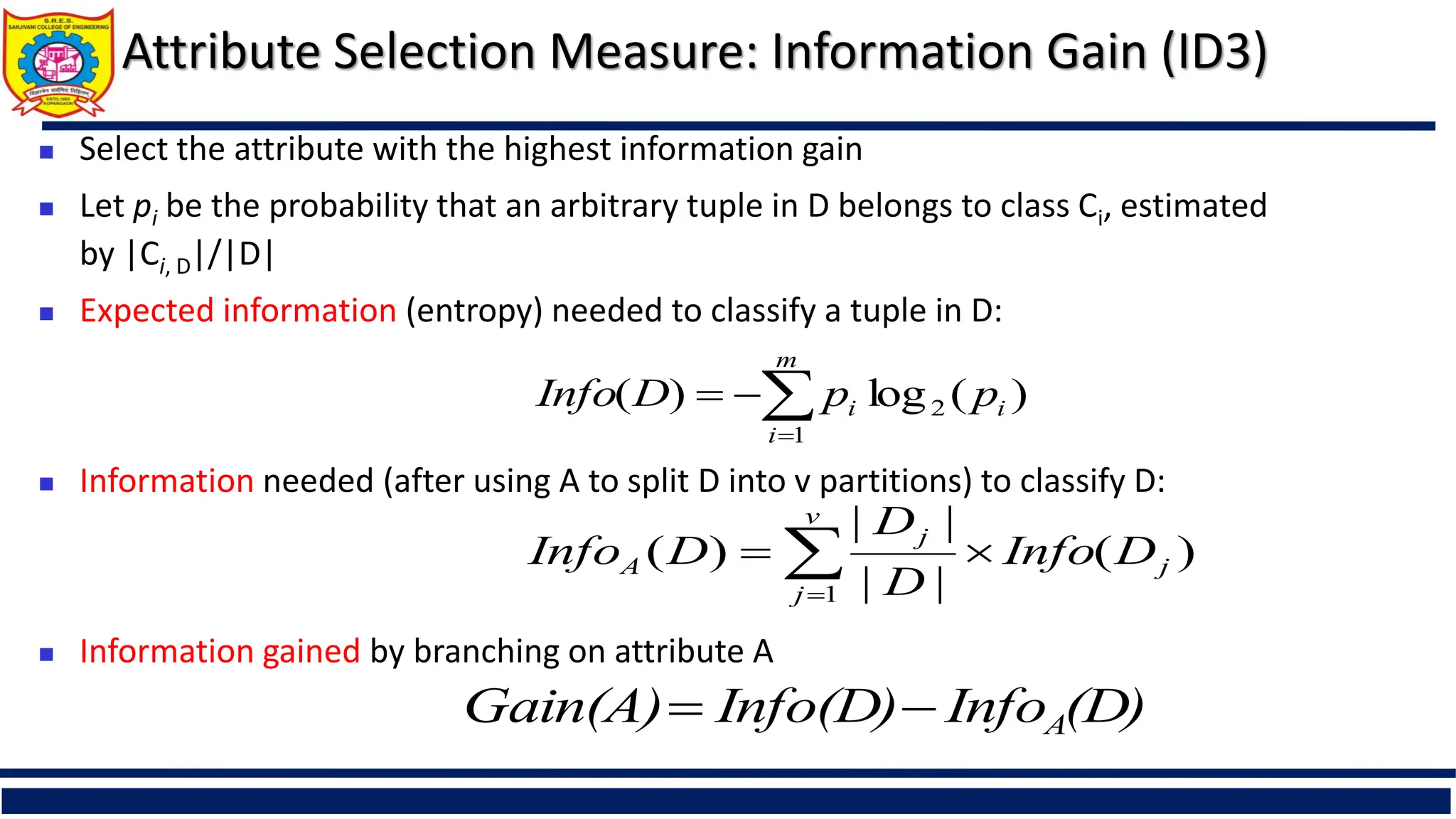
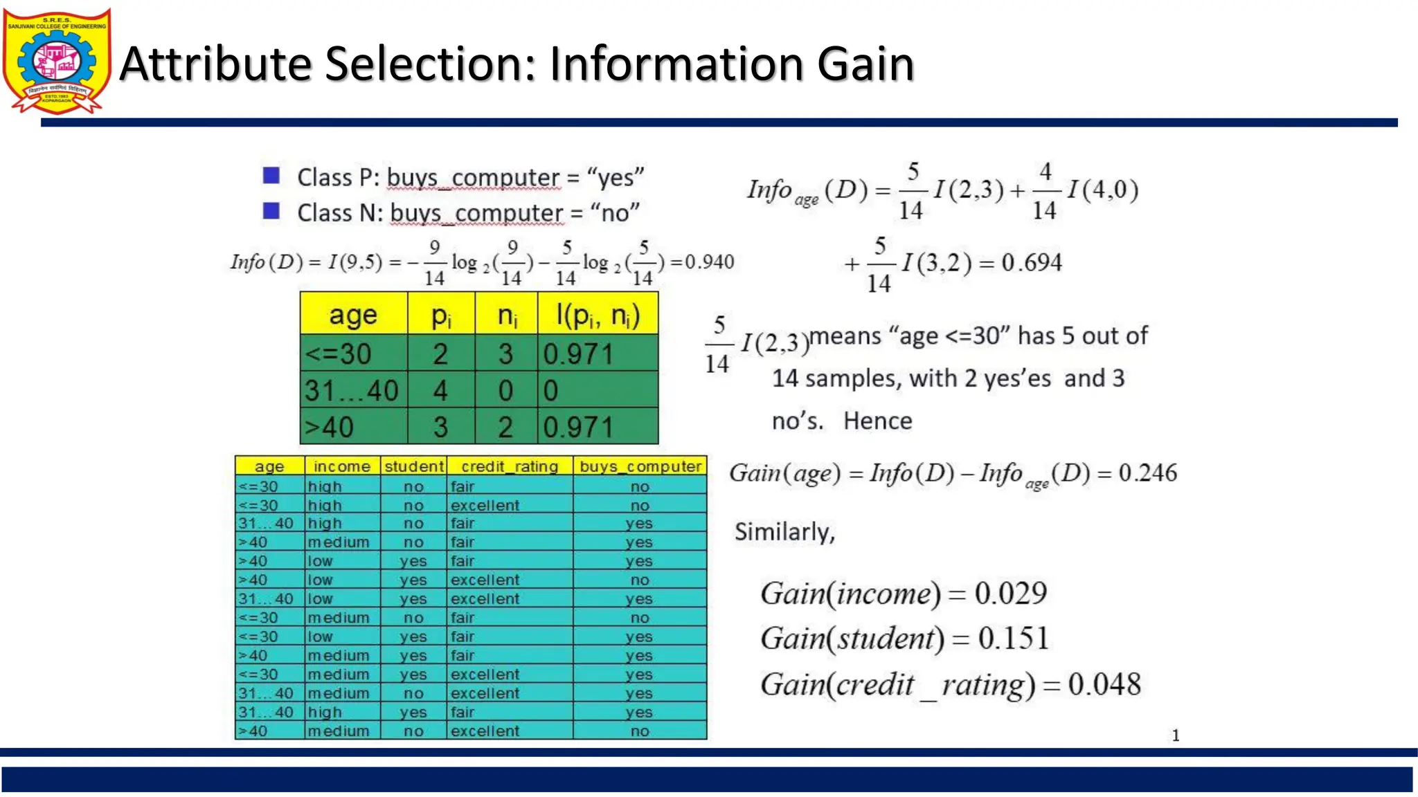
Attribute Selection Measure:Information Gain (ID3)
Select the attribute with the highest information gain
Let pi be the probability that an arbitrary tuple in D belongs to class Ci, estimated
by |Ci, D|/|D|
Expected information (entropy) needed to classify a tuple in D:
Information needed (after using A to split D into v partitions) to classify D:
Information gained by branching on attribute A
)
(
log
)
( 2
1
i
m
i
i p
p
D
Info
)
(
|
|
|
|
)
(
1
j
v
j
j
A D
Info
D
D
D
Info
(D)
Info
Info(D)
Gain(A) A
Computing Information-Gain forContinuous-Value Attributes
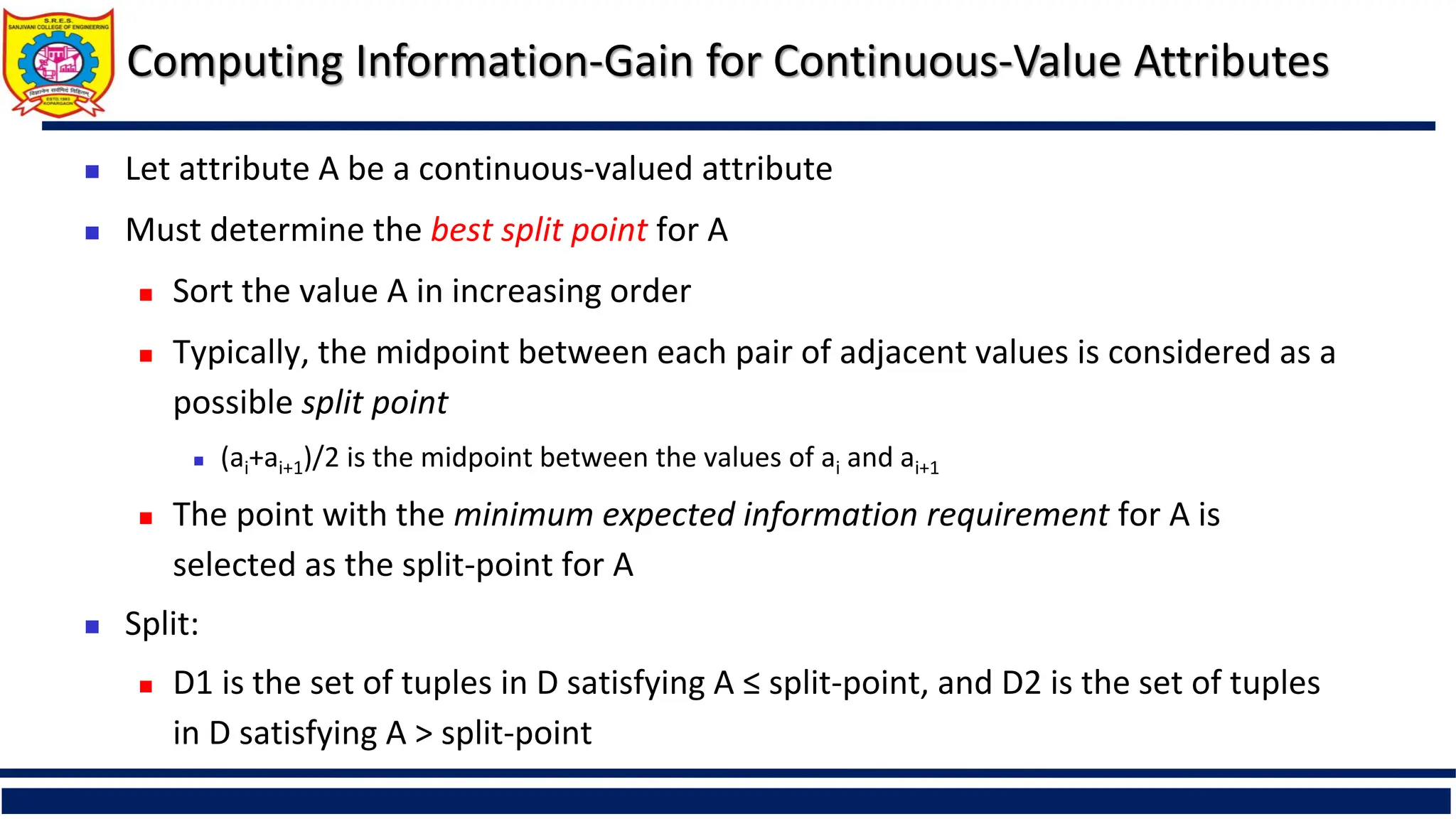
Let attribute A be a continuous-valued attribute
Must determine the best split point for A
Sort the value A in increasing order
Typically, the midpoint between each pair of adjacent values is considered as a
possible split point
(ai+ai+1)/2 is the midpoint between the values of ai and ai+1
The point with the minimum expected information requirement for A is
selected as the split-point for A
Split:
D1 is the set of tuples in D satisfying A ≤ split-point, and D2 is the set of tuples
in D satisfying A > split-point
22.
Gain Ratio forAttribute Selection (C4.5)
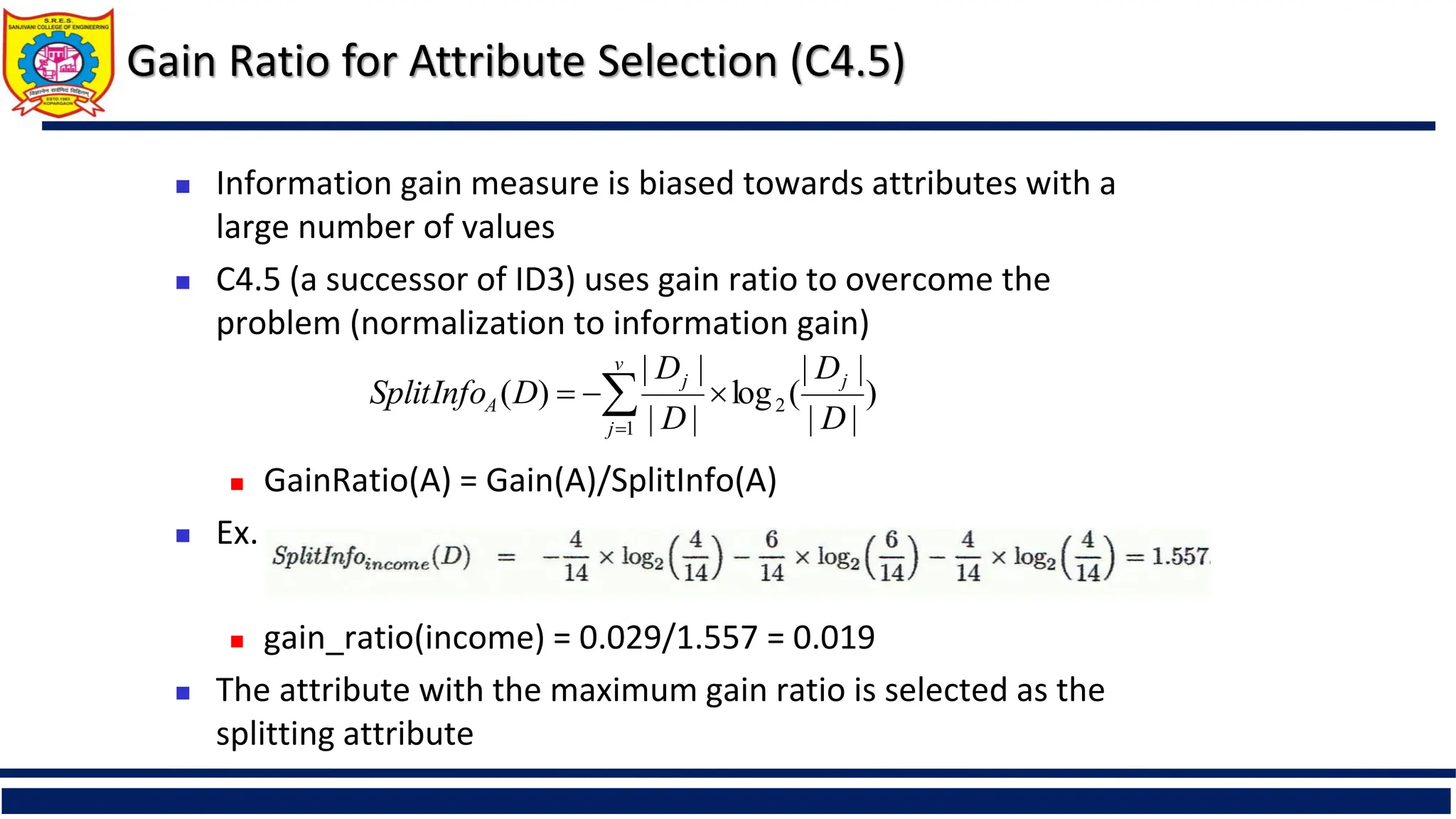
Information gain measure is biased towards attributes with a
large number of values
C4.5 (a successor of ID3) uses gain ratio to overcome the
problem (normalization to information gain)
GainRatio(A) = Gain(A)/SplitInfo(A)
Ex.
gain_ratio(income) = 0.029/1.557 = 0.019
The attribute with the maximum gain ratio is selected as the
splitting attribute
)
|
|
|
|
(
log
|
|
|
|
)
( 2
1 D
D
D
D
D
SplitInfo j
v
j
j
A
23.
Attribute Selection (C4.5):Example 1
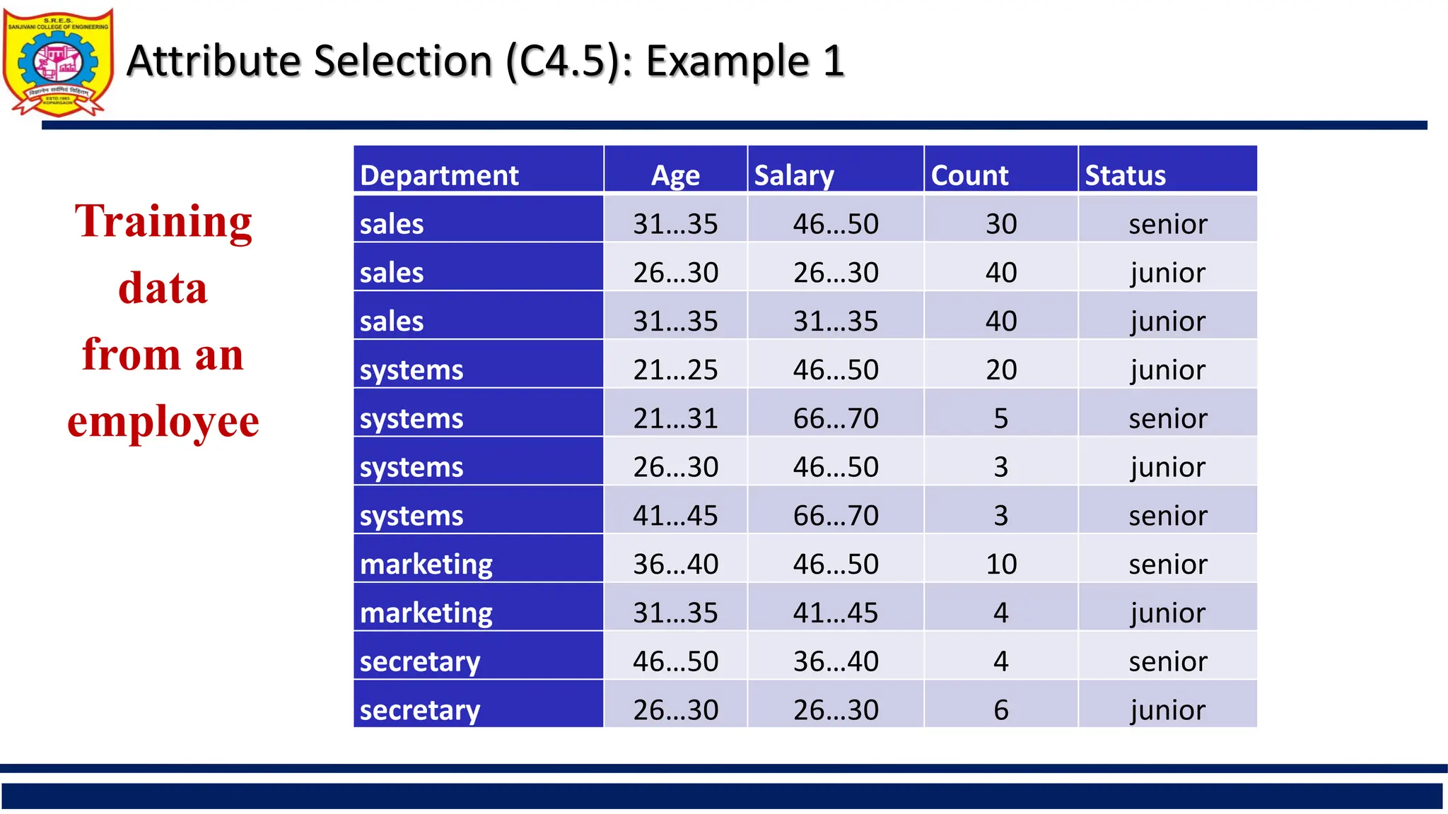
Department Age Salary Count Status
sales 31…35 46…50 30 senior
sales 26…30 26…30 40 junior
sales 31…35 31…35 40 junior
systems 21…25 46…50 20 junior
systems 21…31 66…70 5 senior
systems 26…30 46…50 3 junior
systems 41…45 66…70 3 senior
marketing 36…40 46…50 10 senior
marketing 31…35 41…45 4 junior
secretary 46…50 36…40 4 senior
secretary 26…30 26…30 6 junior
Training
data
from an
employee
24.
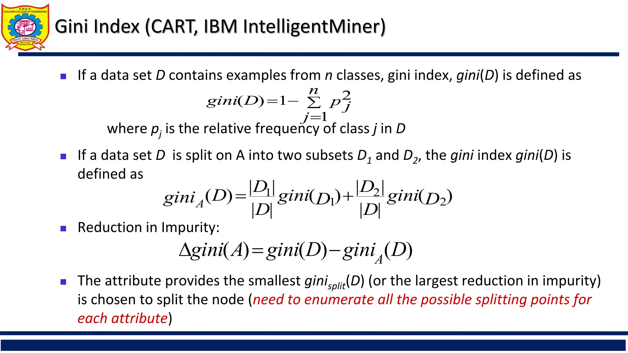
Gini Index (CART,IBM IntelligentMiner)
If a data set D contains examples from n classes, gini index, gini(D) is defined as
where pj is the relative frequency of class j in D
If a data set D is split on A into two subsets D1 and D2, the gini index gini(D) is
defined as
Reduction in Impurity:
The attribute provides the smallest ginisplit(D) (or the largest reduction in impurity)
is chosen to split the node (need to enumerate all the possible splitting points for
each attribute)
n
j
p j
D
gini
1
2
1
)
(
)
(
|
|
|
|
)
(
|
|
|
|
)
( 2
2
1
1
D
gini
D
D
D
gini
D
D
D
giniA
)
(
)
(
)
( D
gini
D
gini
A
gini A
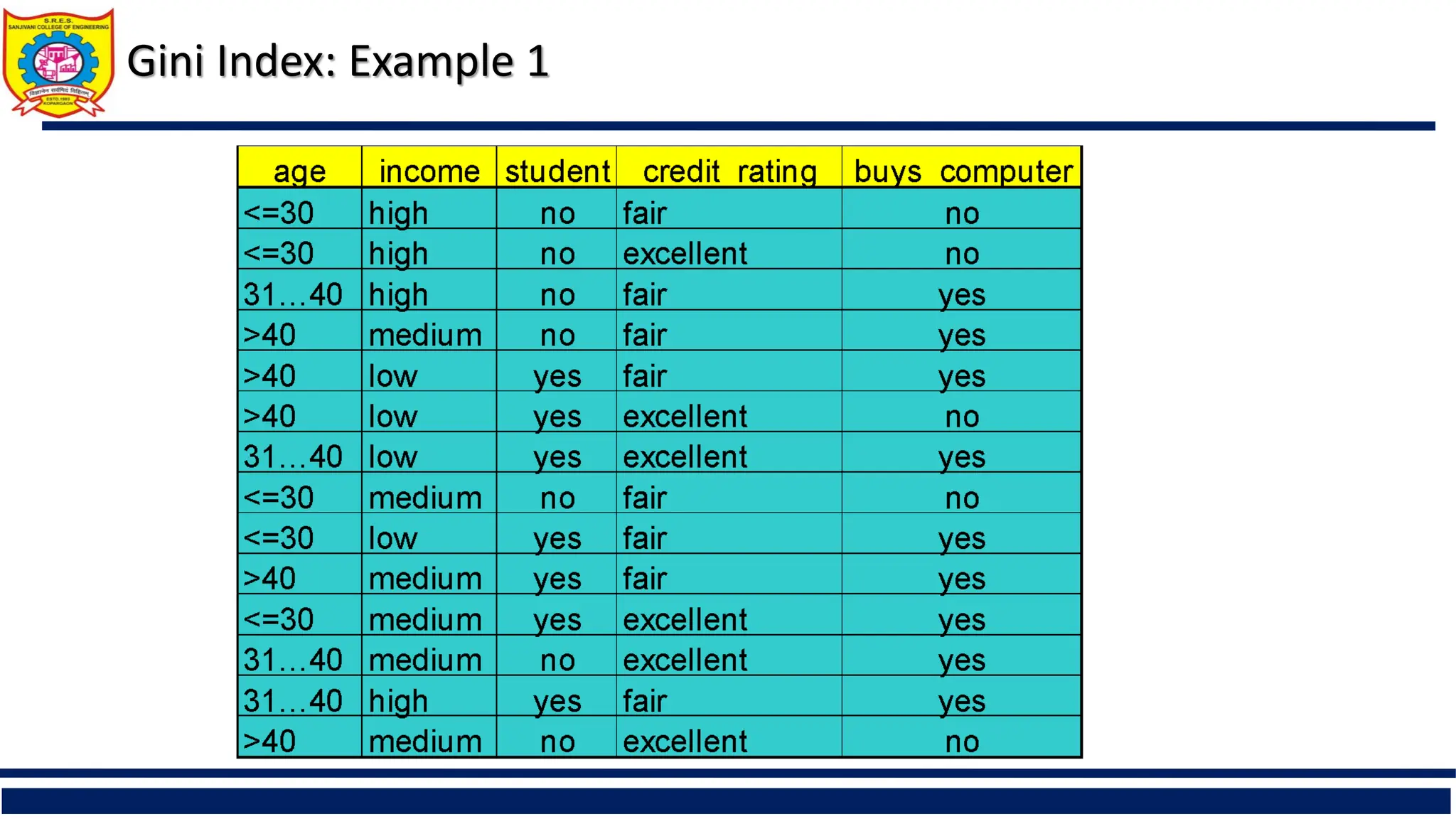
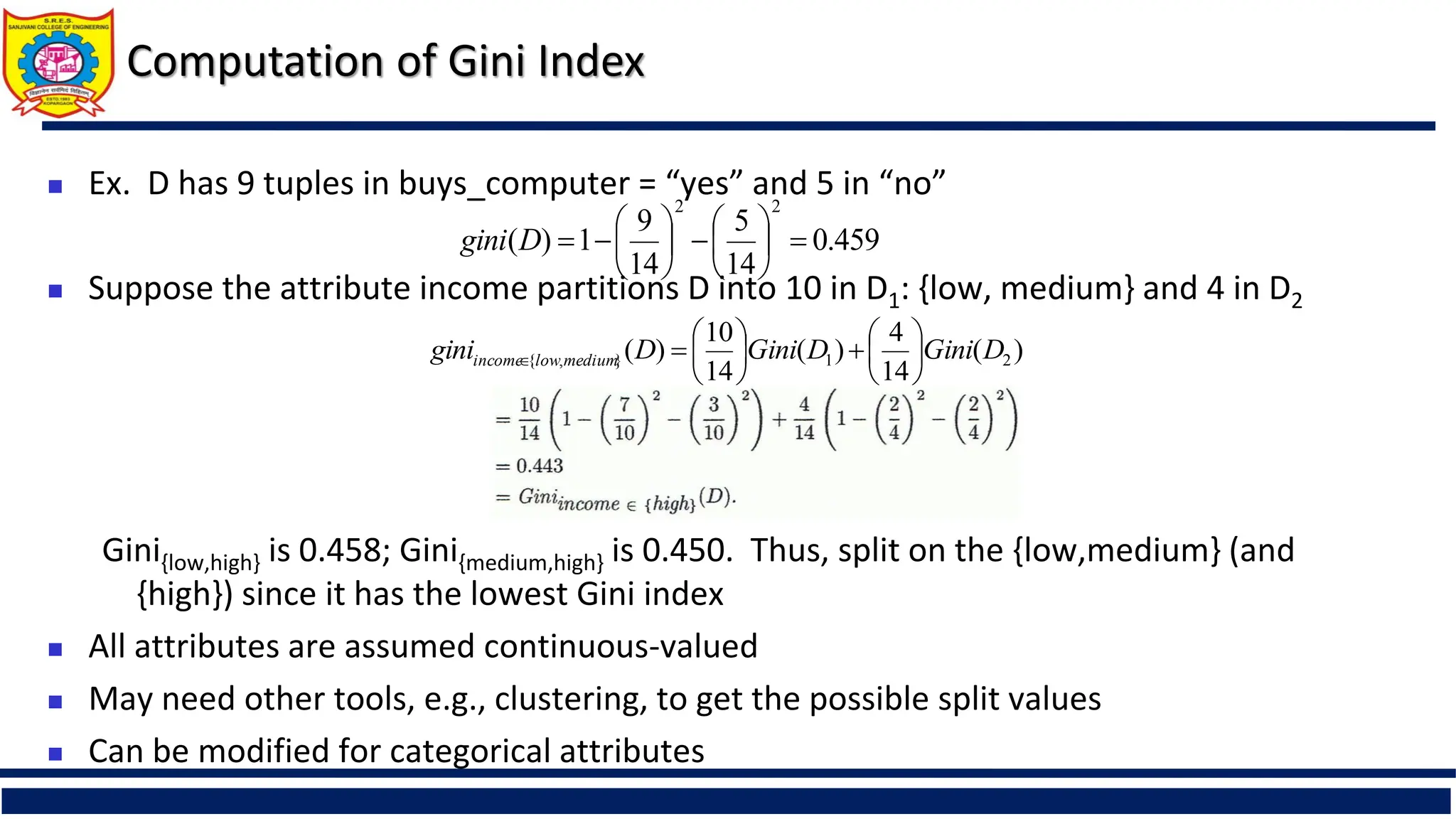
Computation of GiniIndex
Ex. D has 9 tuples in buys_computer = “yes” and 5 in “no”
Suppose the attribute income partitions D into 10 in D1: {low, medium} and 4 in D2
Gini{low,high} is 0.458; Gini{medium,high} is 0.450. Thus, split on the {low,medium} (and
{high}) since it has the lowest Gini index
All attributes are assumed continuous-valued
May need other tools, e.g., clustering, to get the possible split values
Can be modified for categorical attributes
459
.
0
14
5
14
9
1
)
(
2
2
D
gini
)
(
14
4
)
(
14
10
)
( 2
1
}
,
{ D
Gini
D
Gini
D
gini medium
low
income
27.
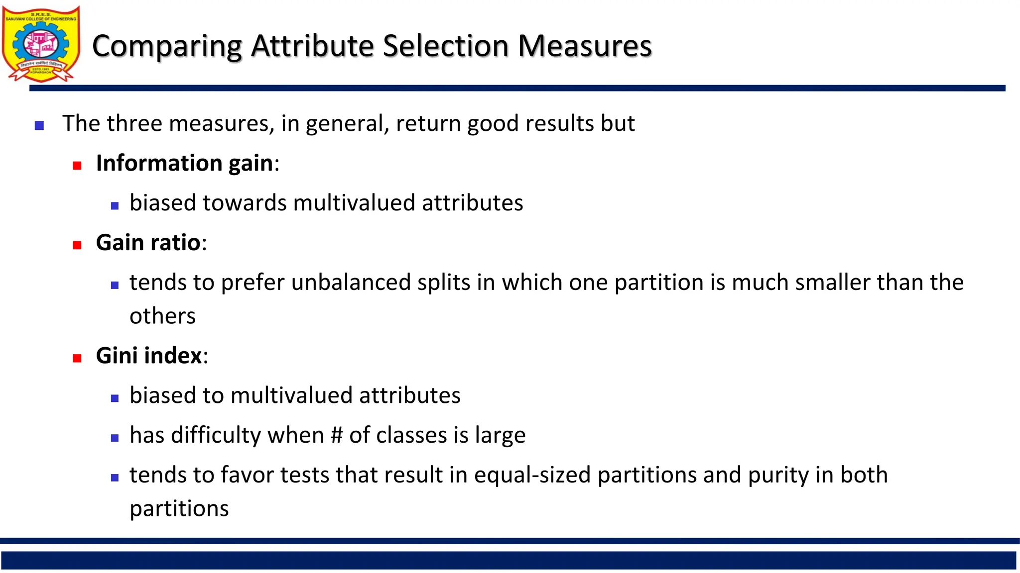
Comparing Attribute SelectionMeasures
The three measures, in general, return good results but
Information gain:
biased towards multivalued attributes
Gain ratio:
tends to prefer unbalanced splits in which one partition is much smaller than the
others
Gini index:
biased to multivalued attributes
has difficulty when # of classes is large
tends to favor tests that result in equal-sized partitions and purity in both
partitions
28.
Other Attribute SelectionMeasures
CHAID: a popular decision tree algorithm, measure based on χ2 test for independence
C-SEP: performs better than info. gain and gini index in certain cases
G-statistic: has a close approximation to χ2 distribution
MDL (Minimal Description Length) principle (i.e., the simplest solution is preferred):
The best tree as the one that requires the fewest # of bits to both (1) encode the tree,
and (2) encode the exceptions to the tree
Multivariate splits (partition based on multiple variable combinations)
CART: finds multivariate splits based on a linear comb. of attrs.
Which attribute selection measure is the best?
Most give good results, none is significantly superior than others
29.
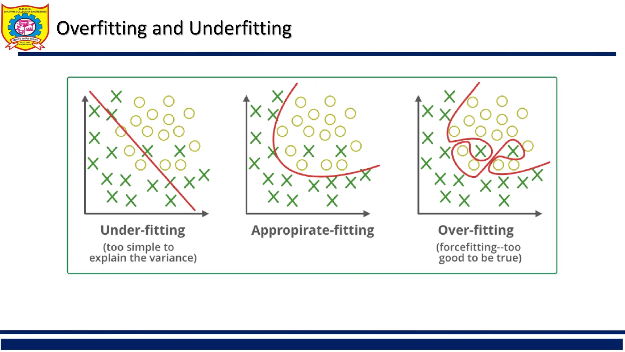
Overfitting: Aninduced tree may overfit the training data
Model tries to accommodate all data points.
Too many branches, some may reflect anomalies due to noise or outliers
Poor accuracy for unseen samples
A solution to avoid overfitting is using a linear algorithm if we have linear data or
using the parameters like the maximal depth if we are using decision trees.
Two approaches to avoid overfitting
Prepruning: Halt tree construction early ̵ do not split a node if this would result in the goodness
measure falling below a threshold
Difficult to choose an appropriate threshold
Postpruning: Remove branches from a “fully grown” tree—get a sequence of progressively
pruned trees
Use a set of data different from the training data to decide which is the “best pruned tree”
Overfitting and Tree Pruning
30.
Underfitting: Aninduced tree may overfit the training data
Model tries to accommodate very few data points e.g. 10% dataset for training and 90 % for
testing.
It has very less accuracy.
An underfit model’s are inaccurate, especially when applied to new,
unseen examples.
Techniques to Reduce Underfitting
Increase model complexity.
Increase the number of features, performing feature engineering.
Remove noise from the data.
Increase the number of epochs or increase the duration of training to get better results.
Overfitting and Tree Pruning
31.
Overfitting and Underfitting
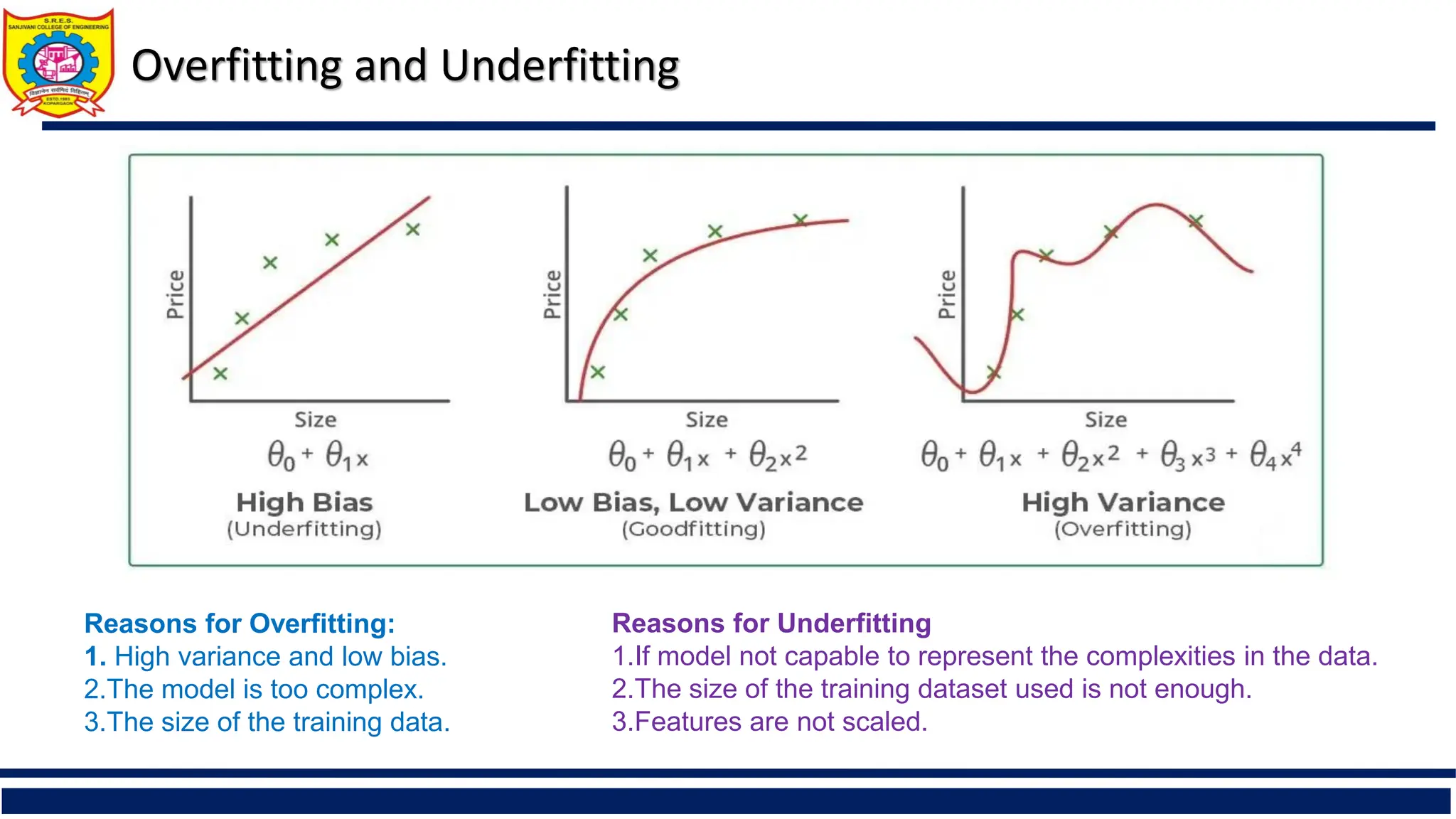
Reasonsfor Overfitting:
1. High variance and low bias.
2.The model is too complex.
3.The size of the training data.
Reasons for Underfitting
1.If model not capable to represent the complexities in the data.
2.The size of the training dataset used is not enough.
3.Features are not scaled.
Enhancements to BasicDecision Tree Induction
Allow for continuous-valued attributes
Dynamically define new discrete-valued attributes that
partition the continuous attribute value into a discrete set of
intervals
Handle missing attribute values
Assign the most common value of the attribute
Assign probability to each of the possible values
Attribute construction
Create new attributes based on existing ones that are
sparsely represented
This reduces fragmentation, repetition, and replication
34.
Bayesian Classification: Why?
A statistical classifier: performs probabilistic prediction, i.e., predicts class
membership probabilities
Foundation: Based on Bayes’ Theorem.
Performance: A simple Bayesian classifier, naïve Bayesian classifier, has comparable
performance with decision tree and selected neural network classifiers
Incremental: Each training example can incrementally increase/decrease the
probability that a hypothesis is correct — prior knowledge can be combined with
observed data
Standard: Even when Bayesian methods are computationally intractable, they can
provide a standard of optimal decision making against which other methods can be
measured
35.
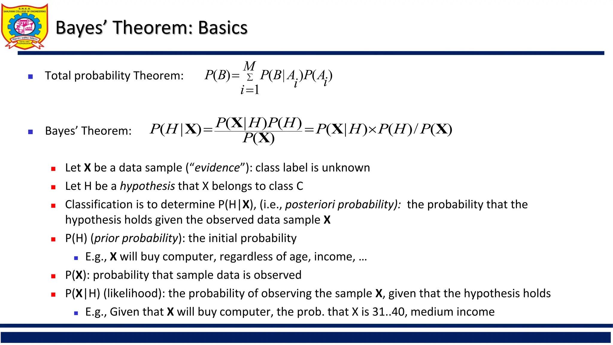
Bayes’ Theorem: Basics
Total probability Theorem:
Bayes’ Theorem:
Let X be a data sample (“evidence”): class label is unknown
Let H be a hypothesis that X belongs to class C
Classification is to determine P(H|X), (i.e., posteriori probability): the probability that the
hypothesis holds given the observed data sample X
P(H) (prior probability): the initial probability
E.g., X will buy computer, regardless of age, income, …
P(X): probability that sample data is observed
P(X|H) (likelihood): the probability of observing the sample X, given that the hypothesis holds
E.g., Given that X will buy computer, the prob. that X is 31..40, medium income
)
(
)
1
|
(
)
( i
A
P
M
i i
A
B
P
B
P
)
(
/
)
(
)
|
(
)
(
)
(
)
|
(
)
|
( X
X
X
X
X P
H
P
H
P
P
H
P
H
P
H
P
36.
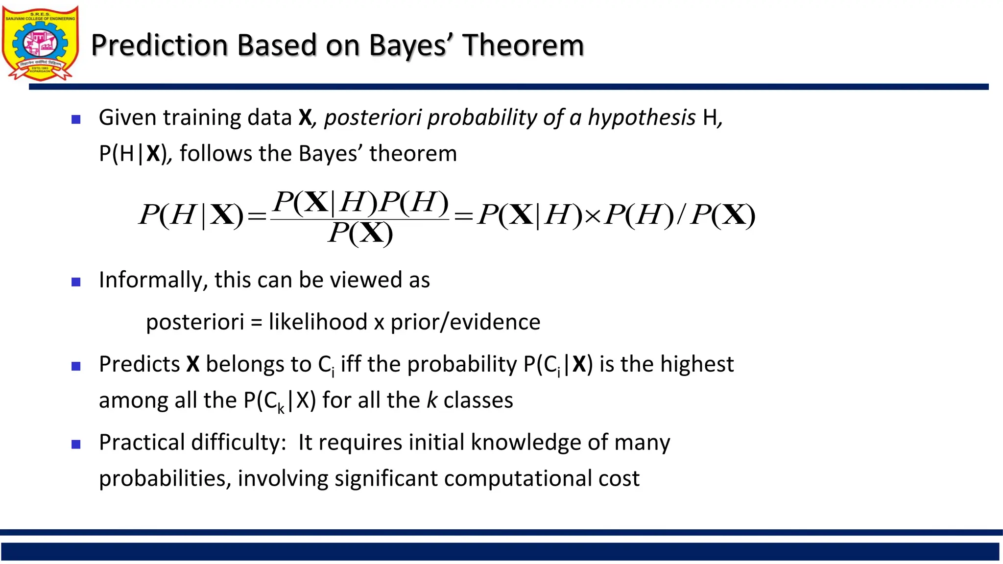
Prediction Based onBayes’ Theorem
Given training data X, posteriori probability of a hypothesis H,
P(H|X), follows the Bayes’ theorem
Informally, this can be viewed as
posteriori = likelihood x prior/evidence
Predicts X belongs to Ci iff the probability P(Ci|X) is the highest
among all the P(Ck|X) for all the k classes
Practical difficulty: It requires initial knowledge of many
probabilities, involving significant computational cost
)
(
/
)
(
)
|
(
)
(
)
(
)
|
(
)
|
( X
X
X
X
X P
H
P
H
P
P
H
P
H
P
H
P
37.
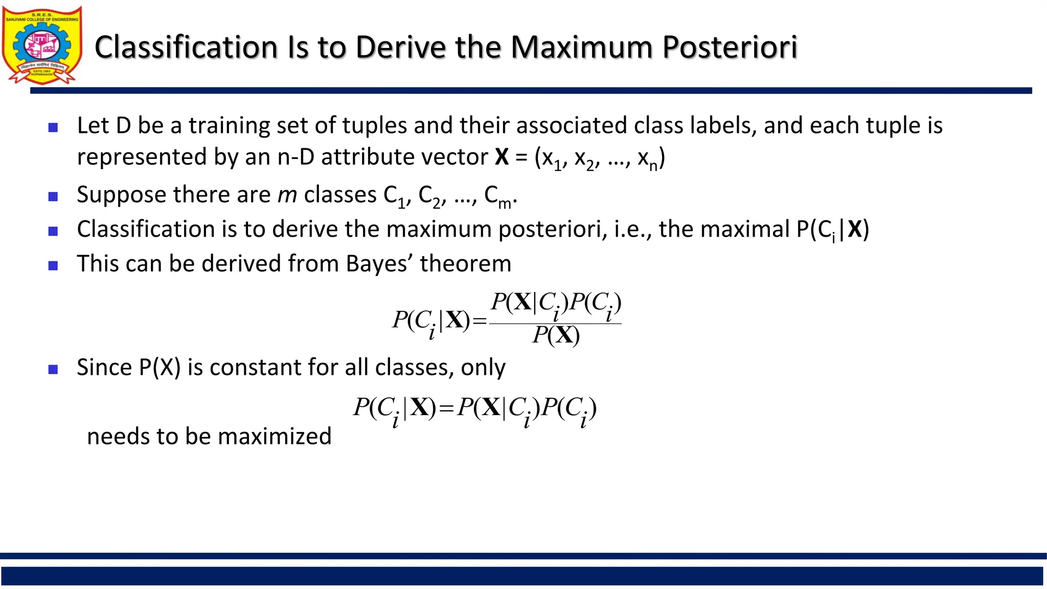
Classification Is toDerive the Maximum Posteriori
Let D be a training set of tuples and their associated class labels, and each tuple is
represented by an n-D attribute vector X = (x1, x2, …, xn)
Suppose there are m classes C1, C2, …, Cm.
Classification is to derive the maximum posteriori, i.e., the maximal P(Ci|X)
This can be derived from Bayes’ theorem
Since P(X) is constant for all classes, only
needs to be maximized
)
(
)
(
)
|
(
)
|
(
X
X
X
P
i
C
P
i
C
P
i
C
P
)
(
)
|
(
)
|
( i
C
P
i
C
P
i
C
P X
X
38.
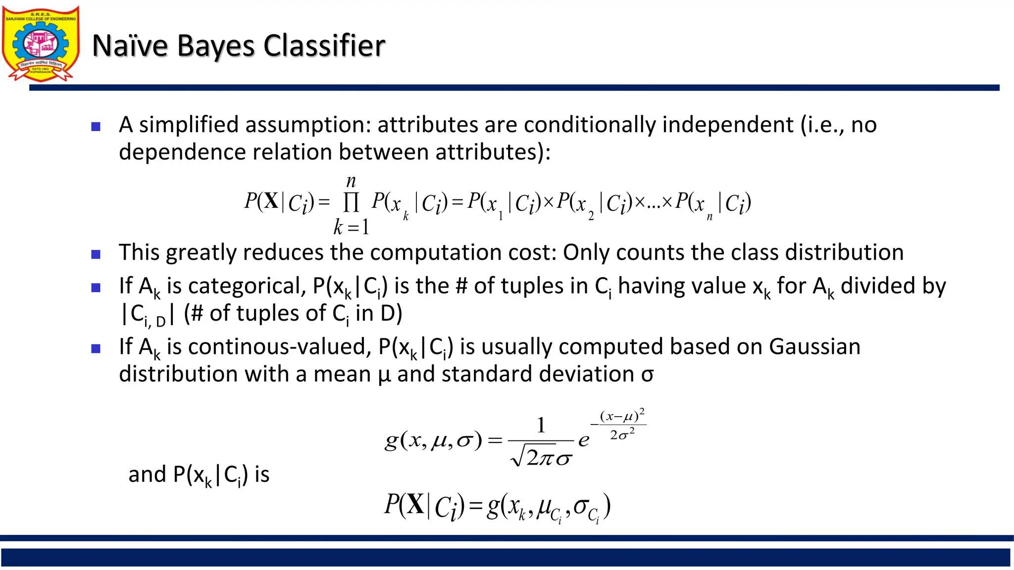
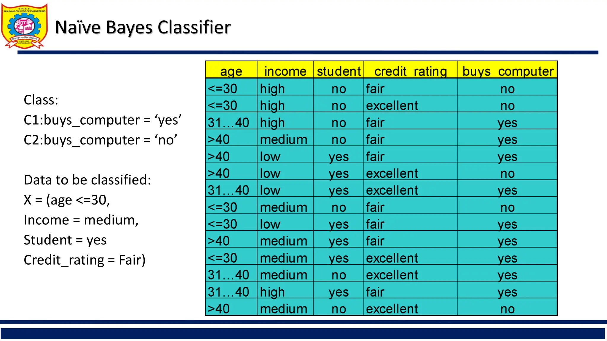
Naïve Bayes Classifier
A simplified assumption: attributes are conditionally independent (i.e., no
dependence relation between attributes):
This greatly reduces the computation cost: Only counts the class distribution
If Ak is categorical, P(xk|Ci) is the # of tuples in Ci having value xk for Ak divided by
|Ci, D| (# of tuples of Ci in D)
If Ak is continous-valued, P(xk|Ci) is usually computed based on Gaussian
distribution with a mean μ and standard deviation σ
and P(xk|Ci) is
)
|
(
...
)
|
(
)
|
(
1
)
|
(
)
|
(
2
1
Ci
x
P
Ci
x
P
Ci
x
P
n
k
Ci
x
P
Ci
P
n
k
X
2
2
2
)
(
2
1
)
,
,
(
x
e
x
g
)
,
,
(
)
|
( i
i C
C
k
x
g
Ci
P
X
Model Evaluation
Evaluationmetrics: How can we measure accuracy? Other
metrics to consider?
Use validation test set of class-labeled tuples instead of
training set when assessing accuracy
Methods for estimating a classifier’s accuracy:
Holdout method, random subsampling
Cross-validation
Bootstrap
Comparing classifiers:
Confidence intervals
Cost-benefit analysis and ROC Curves
41.
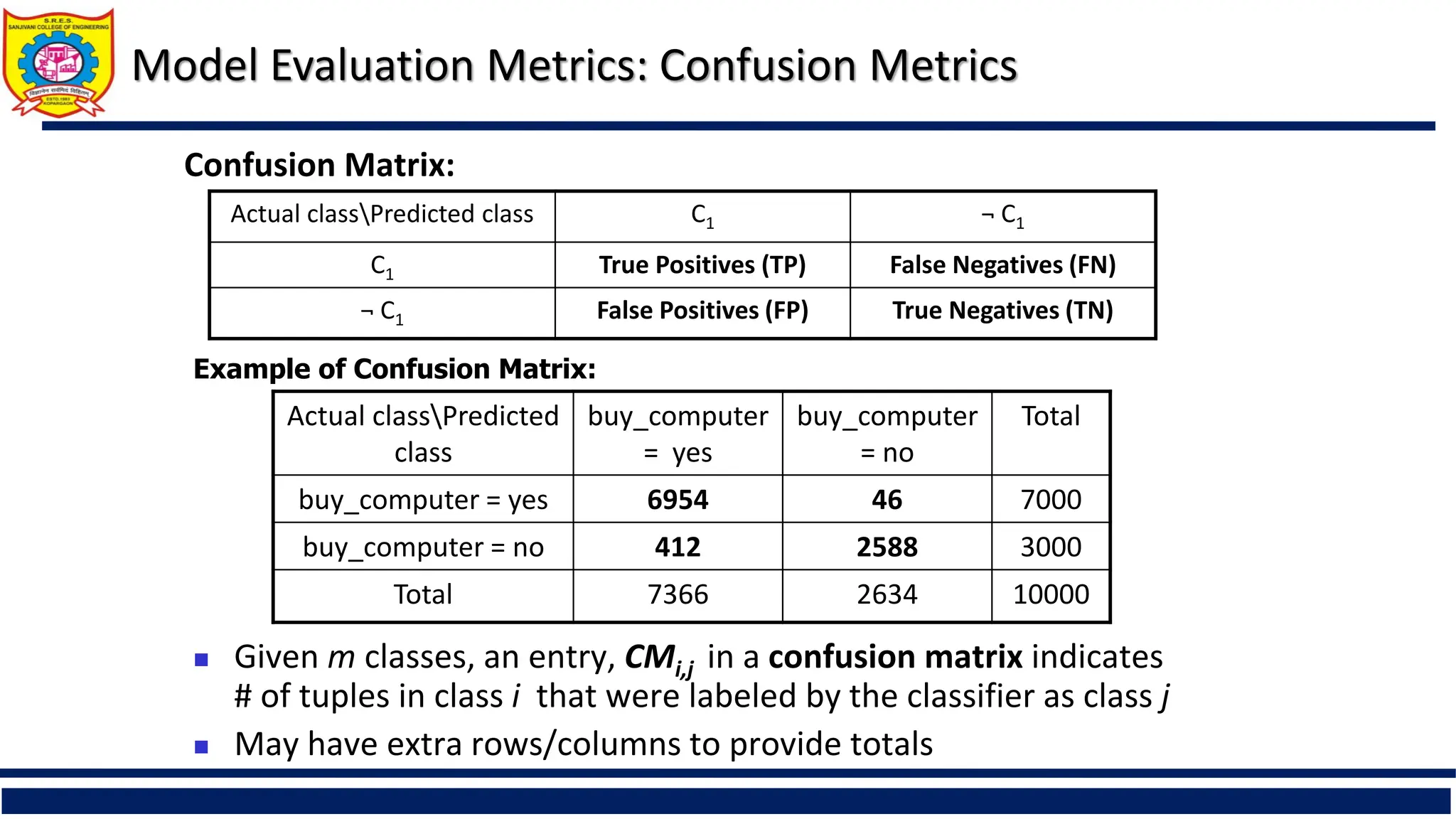
Model Evaluation Metrics:Confusion Metrics
Actual classPredicted
class
buy_computer
= yes
buy_computer
= no
Total
buy_computer = yes 6954 46 7000
buy_computer = no 412 2588 3000
Total 7366 2634 10000
Given m classes, an entry, CMi,j in a confusion matrix indicates
# of tuples in class i that were labeled by the classifier as class j
May have extra rows/columns to provide totals
Confusion Matrix:
Actual classPredicted class C1 ¬ C1
C1 True Positives (TP) False Negatives (FN)
¬ C1 False Positives (FP) True Negatives (TN)
Example of Confusion Matrix:
42.
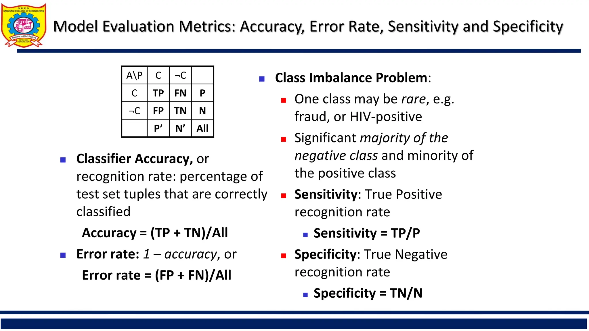
Model Evaluation Metrics:Accuracy, Error Rate, Sensitivity and Specificity
Classifier Accuracy, or
recognition rate: percentage of
test set tuples that are correctly
classified
Accuracy = (TP + TN)/All
Error rate: 1 – accuracy, or
Error rate = (FP + FN)/All
Class Imbalance Problem:
One class may be rare, e.g.
fraud, or HIV-positive
Significant majority of the
negative class and minority of
the positive class
Sensitivity: True Positive
recognition rate
Sensitivity = TP/P
Specificity: True Negative
recognition rate
Specificity = TN/N
AP C ¬C
C TP FN P
¬C FP TN N
P’ N’ All
43.
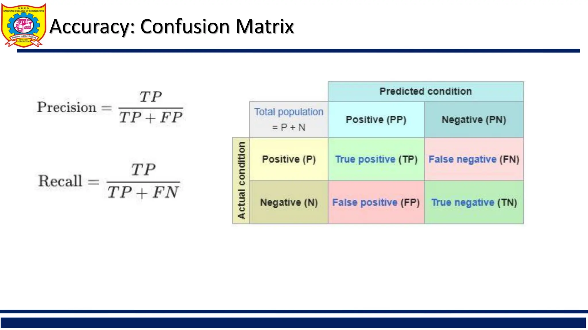
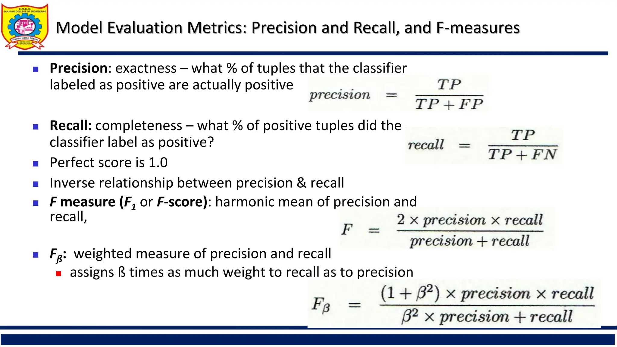
Model Evaluation Metrics:Precision and Recall, and F-measures
Precision: exactness – what % of tuples that the classifier
labeled as positive are actually positive
Recall: completeness – what % of positive tuples did the
classifier label as positive?
Perfect score is 1.0
Inverse relationship between precision & recall
F measure (F1 or F-score): harmonic mean of precision and
recall,
Fß: weighted measure of precision and recall
assigns ß times as much weight to recall as to precision
44.
Lazy vs. EagerLearning
Lazy vs. eager learning
Lazy learning (e.g., instance-based learning): Simply
stores training data (or only minor processing) and
waits until it is given a test tuple
Eager learning (the above discussed methods): Given
a set of training tuples, constructs a classification model
before receiving new (e.g., test) data to classify
Lazy: less time in training but more time in predicting
Accuracy
Lazy method effectively uses a richer hypothesis space
since it uses many local linear functions to form an
implicit global approximation to the target function
Eager: must commit to a single hypothesis that covers
the entire instance space
45.
Lazy Learner: Instance-BasedMethods
Instance-based learning:
Store training examples and delay the processing (“lazy
evaluation”) until a new instance must be classified
Typical approaches
k-nearest neighbor approach
Instances represented as points in a Euclidean space.
Locally weighted regression
Constructs local approximation
Case-based reasoning
Uses symbolic representations and knowledge-based
inference
46.
The k-Nearest NeighborAlgorithm
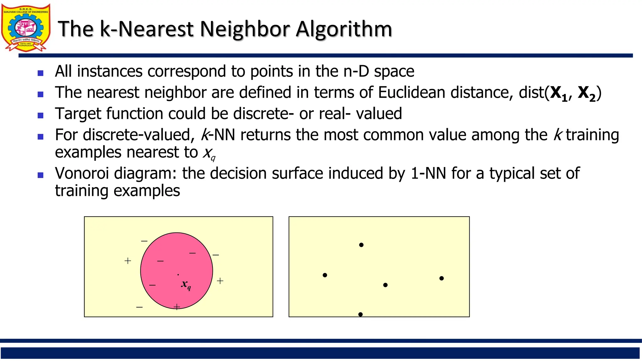
All instances correspond to points in the n-D space
The nearest neighbor are defined in terms of Euclidean distance, dist(X1, X2)
Target function could be discrete- or real- valued
For discrete-valued, k-NN returns the most common value among the k training
examples nearest to xq
Vonoroi diagram: the decision surface induced by 1-NN for a typical set of
training examples
.
_
_ xq
+
_ _
+
_
_
+
.
.
.
. .
47.
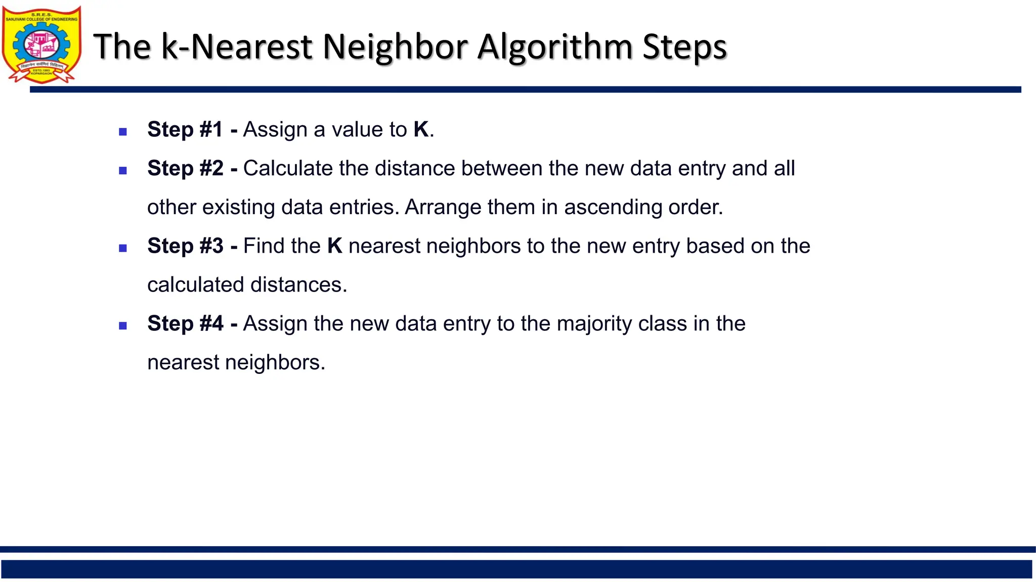
Step #1- Assign a value to K.
Step #2 - Calculate the distance between the new data entry and all
other existing data entries. Arrange them in ascending order.
Step #3 - Find the K nearest neighbors to the new entry based on the
calculated distances.
Step #4 - Assign the new data entry to the majority class in the
nearest neighbors.
The k-Nearest Neighbor Algorithm Steps
48.
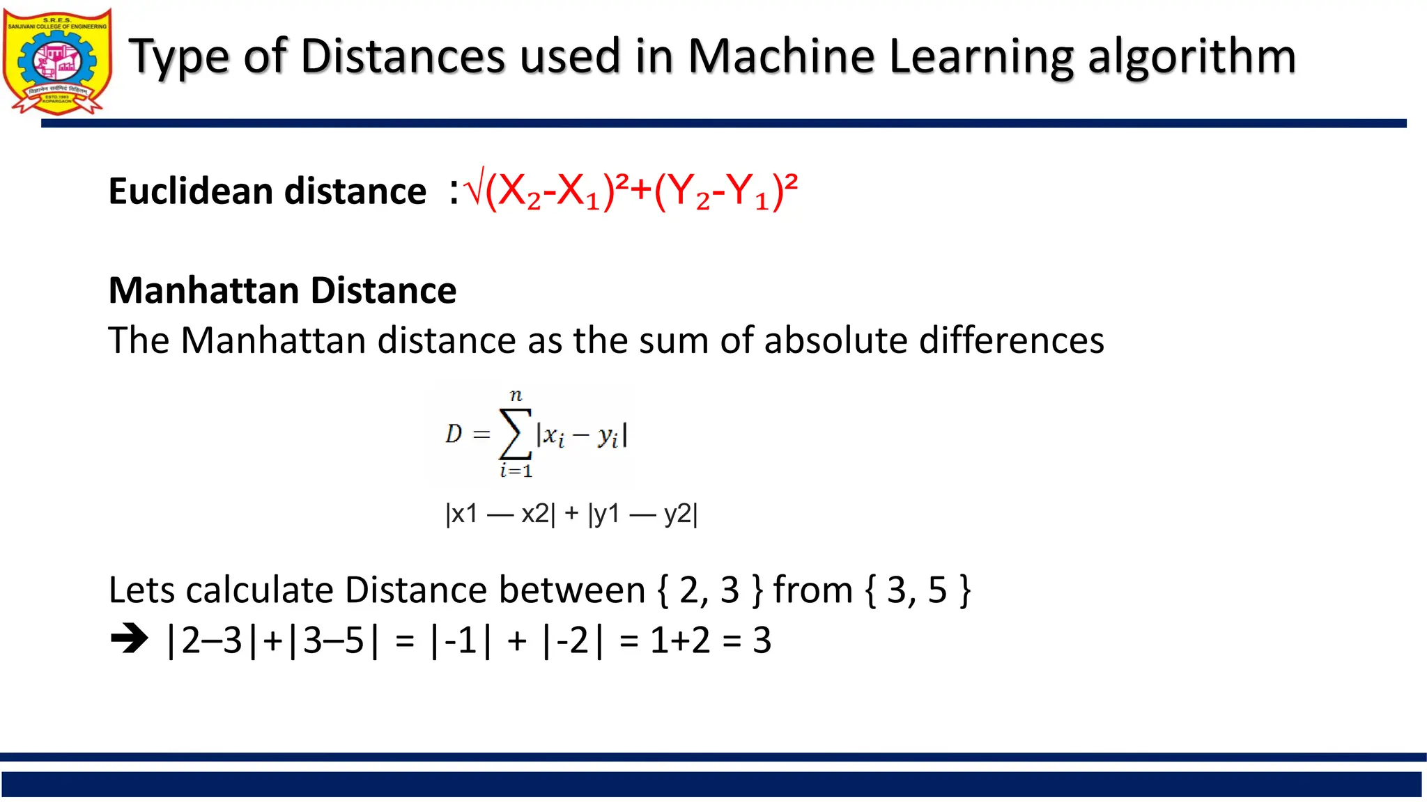
Type of Distancesused in Machine Learning algorithm
Euclidean distance :√(X₂-X₁)²+(Y₂-Y₁)²
Manhattan Distance
The Manhattan distance as the sum of absolute differences
Lets calculate Distance between { 2, 3 } from { 3, 5 }
|2–3|+|3–5| = |-1| + |-2| = 1+2 = 3
|x1 — x2| + |y1 — y2|
49.
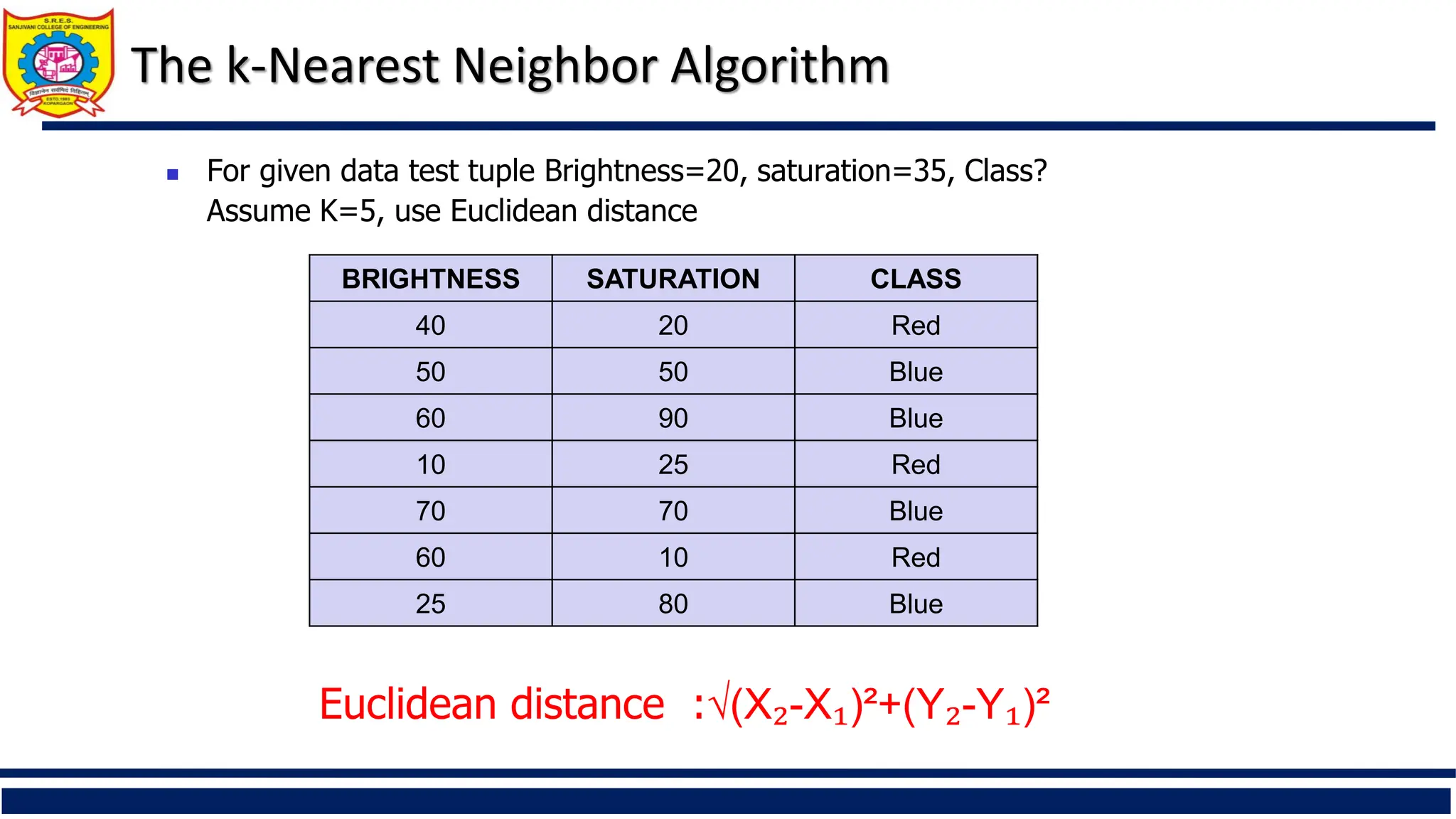
For givendata test tuple Brightness=20, saturation=35, Class?
Assume K=5, use Euclidean distance
BRIGHTNESS SATURATION CLASS
40 20 Red
50 50 Blue
60 90 Blue
10 25 Red
70 70 Blue
60 10 Red
25 80 Blue
Euclidean distance :√(X₂-X₁)²+(Y₂-Y₁)²
The k-Nearest Neighbor Algorithm
50.
What Is Prediction?
(Numerical) prediction is similar to classification
construct a model
use model to predict continuous or ordered value for a given input
Prediction is different from classification
Classification refers to predict categorical class label
Prediction models continuous-valued functions
Major method for prediction: regression
model the relationship between one or more independent or
predictor variables and a dependent or response variable
Regression analysis
Linear and multiple regression
Non-linear regression
Other regression methods: generalized linear model, Poisson
regression, log-linear models, regression trees
51.
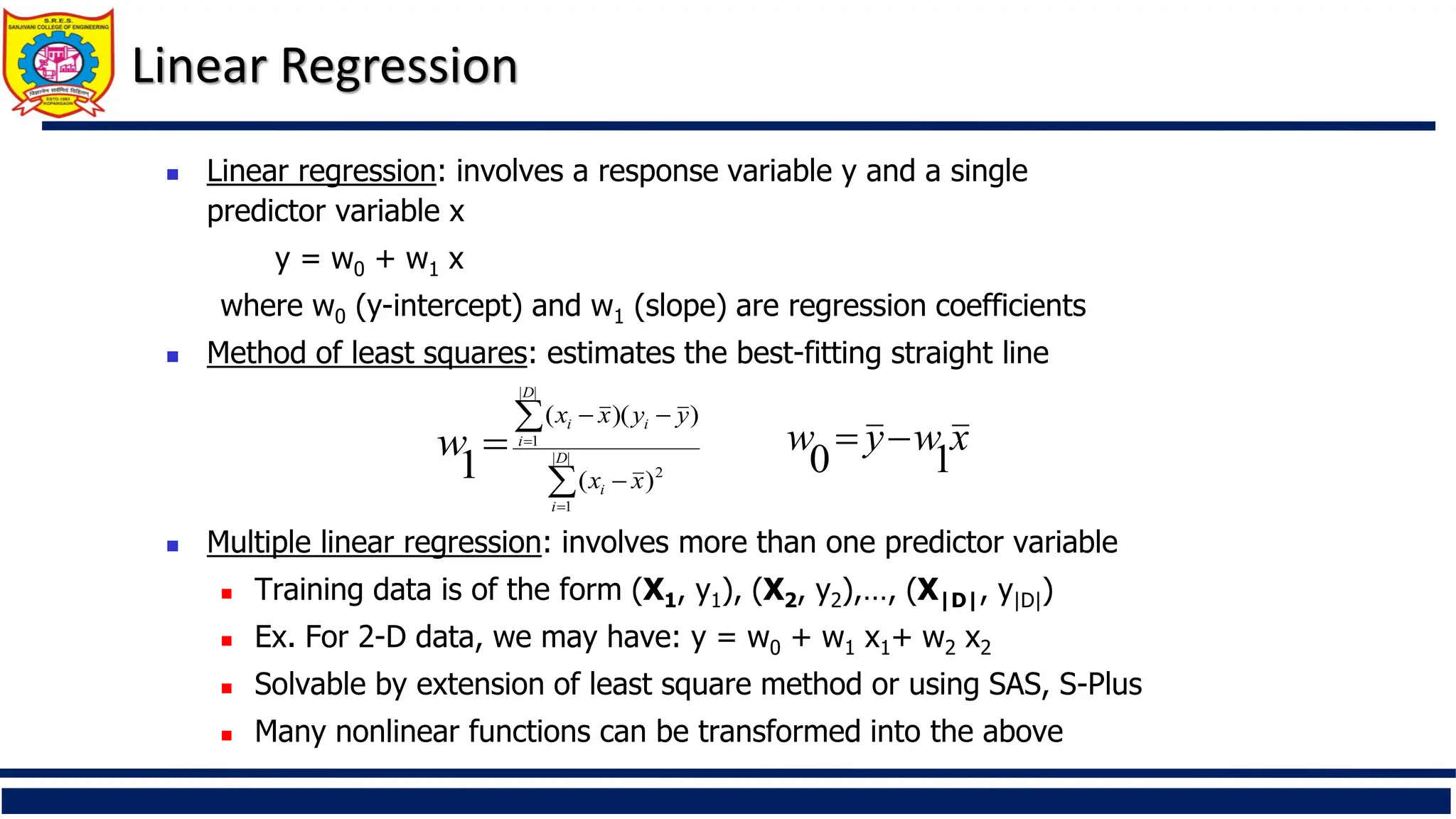
Linear Regression
Linearregression: involves a response variable y and a single
predictor variable x
y = w0 + w1 x
where w0 (y-intercept) and w1 (slope) are regression coefficients
Method of least squares: estimates the best-fitting straight line
Multiple linear regression: involves more than one predictor variable
Training data is of the form (X1, y1), (X2, y2),…, (X|D|, y|D|)
Ex. For 2-D data, we may have: y = w0 + w1 x1+ w2 x2
Solvable by extension of least square method or using SAS, S-Plus
Many nonlinear functions can be transformed into the above
|
|
1
2
|
|
1
)
(
)
)(
(
1 D
i
i
D
i
i
i
x
x
y
y
x
x
w x
w
y
w
1
0
52.
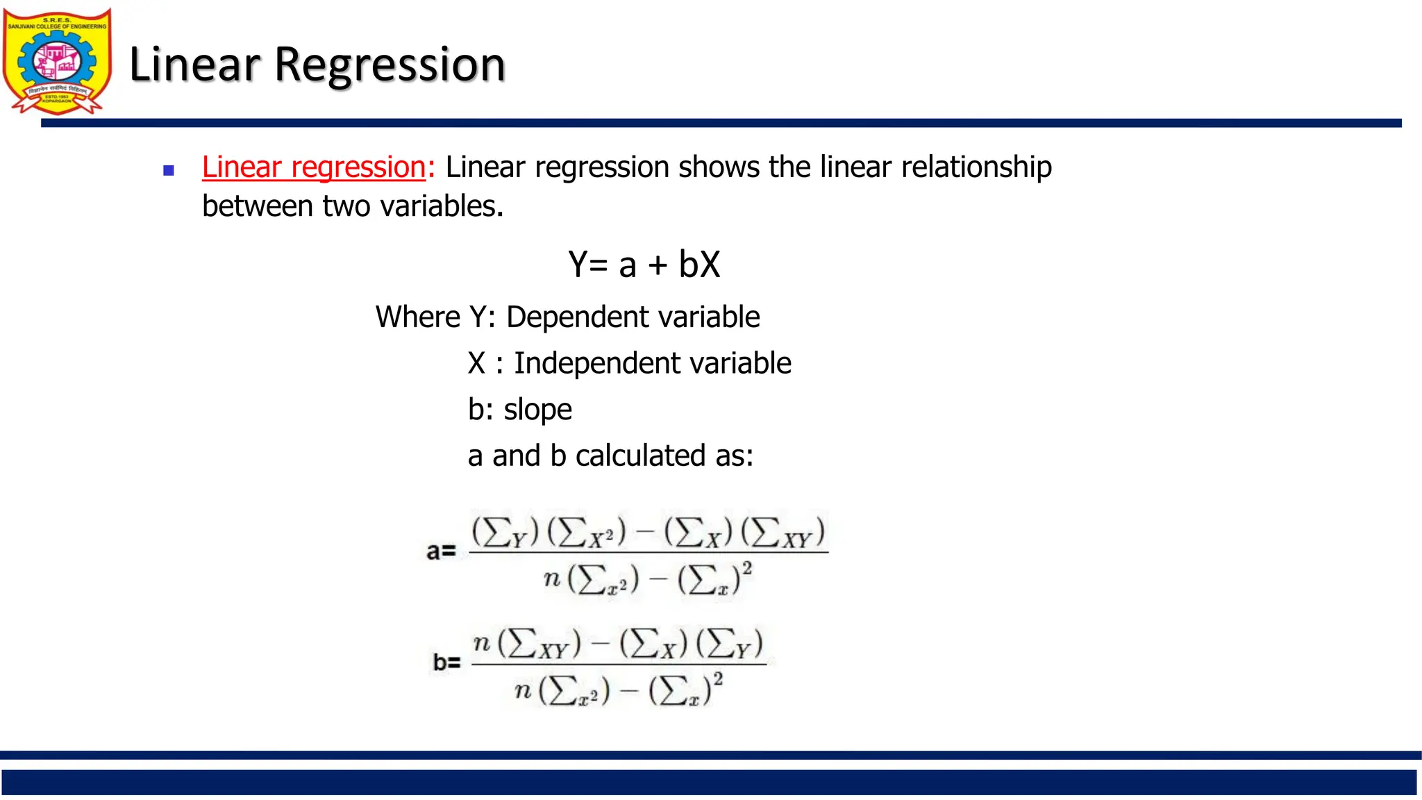
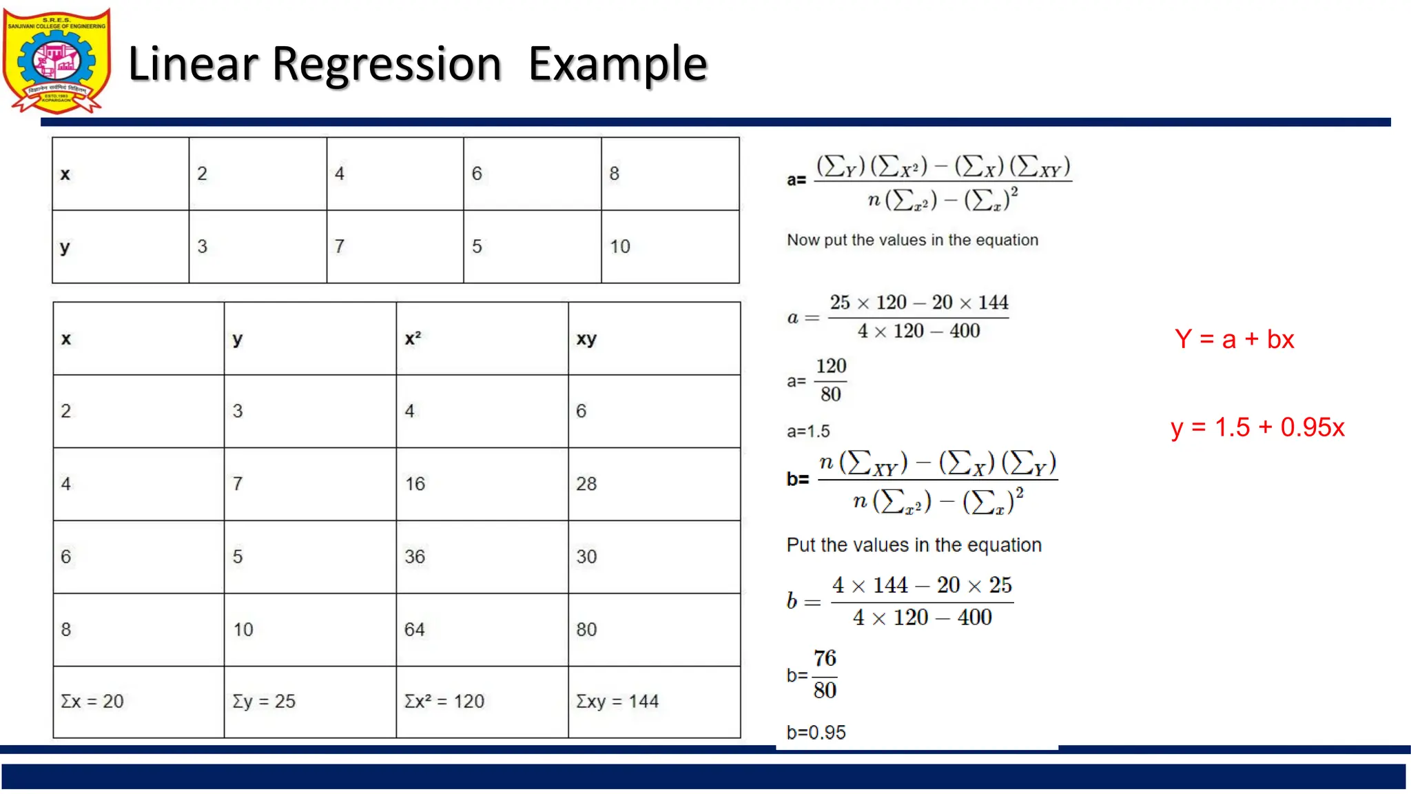
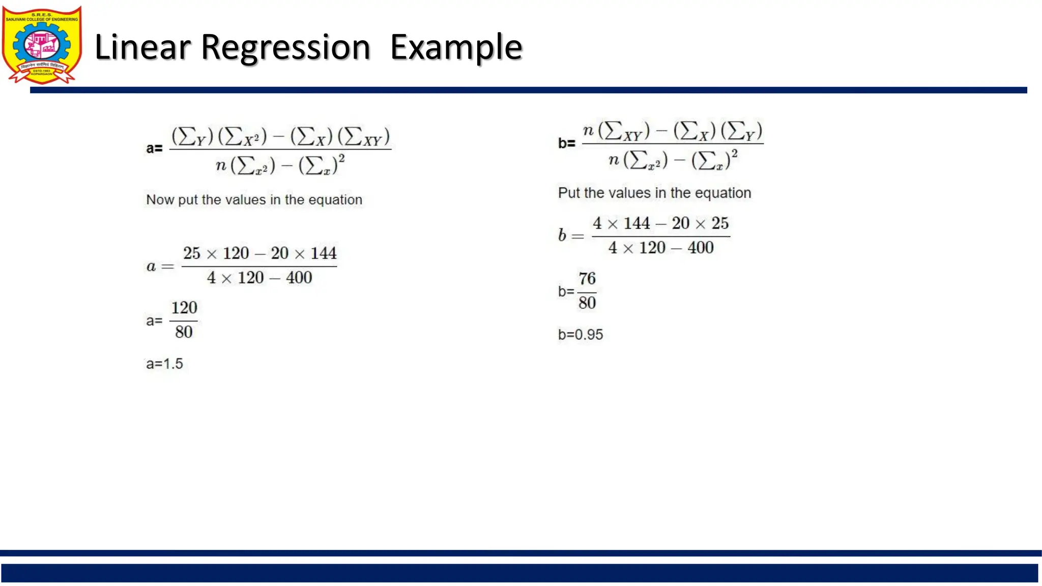
Linear Regression
Linearregression: Linear regression shows the linear relationship
between two variables.
Y= a + bX
Where Y: Dependent variable
X : Independent variable
b: slope
a and b calculated as:
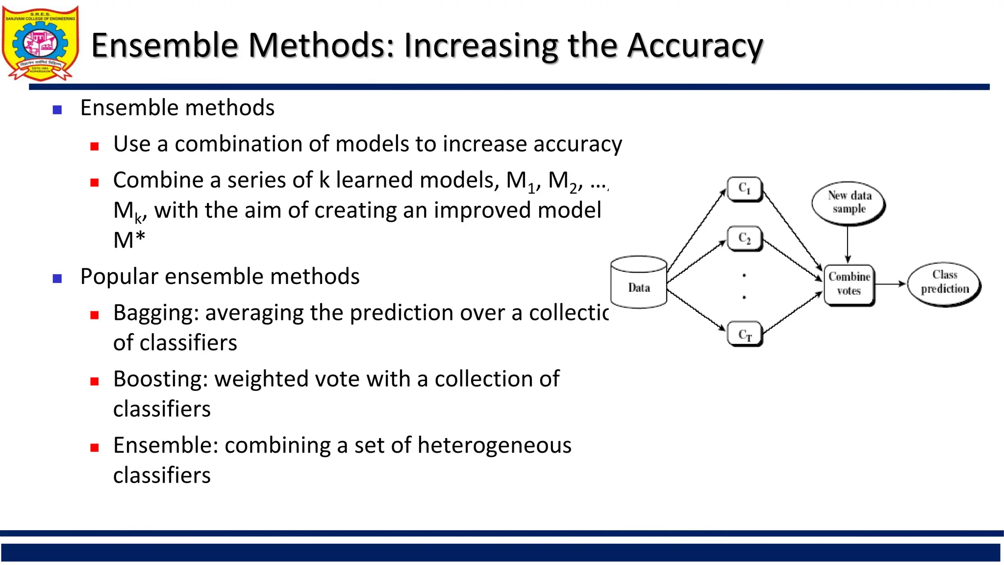
Ensemble Methods: Increasingthe Accuracy
Ensemble methods
Use a combination of models to increase accuracy
Combine a series of k learned models, M1, M2, …,
Mk, with the aim of creating an improved model
M*
Popular ensemble methods
Bagging: averaging the prediction over a collection
of classifiers
Boosting: weighted vote with a collection of
classifiers
Ensemble: combining a set of heterogeneous
classifiers
56.
DEPARTMENT OF COMPUTERENGINEERING, Sanjivani COE, Kopargaon 56
Reference
Han, Jiawei Kamber, Micheline Pei and Jian, “Data Mining: Concepts and
Techniques”,Elsevier Publishers, ISBN:9780123814791, 9780123814807.
https://onlinecourses.nptel.ac.in/noc24_cs22
https://medium.com/analytics-vidhya/type-of-distances-used-in-machine-
learning-algorithm-c873467140de
https://www.freecodecamp.org/news/k-nearest-neighbors-algorithm-
classifiers-and-model-example/