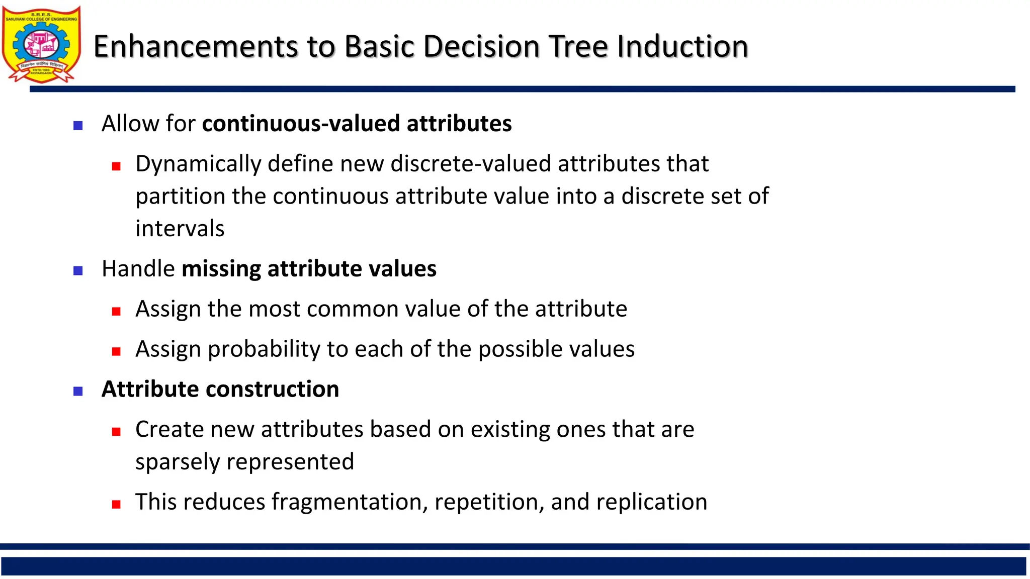
Supervised Learning Decision Trees Machine Learning

Sanjivani Rural Education Society’s
Sanjivani College of Engineering, Kopargaon-423 603
(An Autonomous Institute, Affiliated to Savitribai Phule Pune University, Pune)
NACC ‘A’ Grade Accredited, ISO 9001:2015 Certified
Department of Computer Engineering
(NBA Accredited)
Prof. S. A. Shivarkar
Assistant Professor
Contact No.8275032712
Email- shivarkarsandipcomp@sanjivani.org.in
Subject- Supervised Modeling and AI Technologies (CO9401)
Unit –II: Supervised Learning Decision Trees

Content
 Decision trees, Designing/Building of decision trees, Greedy algorithm,
Decision tree algorithm selection algorithm, Constraints of decision tree
algorithm, Use of Decision tree as a classifier as well as regressor,
 Attribute selection(Entropy, Information gain, GINI index)

Decision Tree Induction: Training Dataset

Decision Tree Induction: Training Dataset
age?
overcast
student? credit rating?
<=30 >40
no yes yes
yes
31..40
fair
excellent
yes
no
 Training data set: Buys_computer
 The data set follows an example of
Quinlan’s ID3 (Playing Tennis)
 Resulting tree:

Algorithm for Decision Tree Induction
 Basic algorithm (a greedy algorithm)
 Tree is constructed in a top-down recursive divide-and-conquer manner
 At start, all the training examples are at the root
 Attributes are categorical (if continuous-valued, they are discretized in
advance)
 Examples are partitioned recursively based on selected attributes
 Test attributes are selected on the basis of a heuristic or statistical measure
(e.g., information gain)
 Conditions for stopping partitioning
 All samples for a given node belong to the same class
 There are no remaining attributes for further partitioning – majority voting
is employed for classifying the leaf
 There are no samples left

Brief Review of Entropy

m = 2

Attribute Selection Measure: Information Gain (ID3)
 Select the attribute with the highest information gain
 Let pi be the probability that an arbitrary tuple in D belongs to class Ci, estimated
by |Ci, D|/|D|
 Expected information (entropy) needed to classify a tuple in D:
 Information needed (after using A to split D into v partitions) to classify D:
 Information gained by branching on attribute A
)
(
log
)
( 2
1
i
m
i
i p
p
D
Info 



)
(
|
|
|
|
)
(
1
j
v
j
j
A D
Info
D
D
D
Info 
 

(D)
Info
Info(D)
Gain(A) A



Decision Tree Induction: Training Dataset Example 1

Attribute Selection: Information Gain

Decision Tree Induction: Training Dataset Example 2

Computing Information-Gain for Continuous-Value Attributes
 Let attribute A be a continuous-valued attribute
 Must determine the best split point for A
 Sort the value A in increasing order
 Typically, the midpoint between each pair of adjacent values is considered as a
possible split point
 (ai+ai+1)/2 is the midpoint between the values of ai and ai+1
 The point with the minimum expected information requirement for A is
selected as the split-point for A
 Split:
 D1 is the set of tuples in D satisfying A ≤ split-point, and D2 is the set of tuples
in D satisfying A > split-point

Gain Ratio for Attribute Selection (C4.5)
 Information gain measure is biased towards attributes with a
large number of values
 C4.5 (a successor of ID3) uses gain ratio to overcome the
problem (normalization to information gain)
 GainRatio(A) = Gain(A)/SplitInfo(A)
 Ex.
 gain_ratio(income) = 0.029/1.557 = 0.019
 The attribute with the maximum gain ratio is selected as the
splitting attribute
)
|
|
|
|
(
log
|
|
|
|
)
( 2
1 D
D
D
D
D
SplitInfo j
v
j
j
A 

 


Attribute Selection (C4.5): Example 1
Department Age Salary Count Status
sales 31…35 46…50 30 senior
sales 26…30 26…30 40 junior
sales 31…35 31…35 40 junior
systems 21…25 46…50 20 junior
systems 21…31 66…70 5 senior
systems 26…30 46…50 3 junior
systems 41…45 66…70 3 senior
marketing 36…40 46…50 10 senior
marketing 31…35 41…45 4 junior
secretary 46…50 36…40 4 senior
secretary 26…30 26…30 6 junior
Training
data
from an
employee

Gini Index (CART, IBM IntelligentMiner)
 If a data set D contains examples from n classes, gini index, gini(D) is defined as
where pj is the relative frequency of class j in D
 If a data set D is split on A into two subsets D1 and D2, the gini index gini(D) is
defined as
 Reduction in Impurity:
 The attribute provides the smallest ginisplit(D) (or the largest reduction in impurity)
is chosen to split the node (need to enumerate all the possible splitting points for
each attribute)




n
j
p j
D
gini
1
2
1
)
(
)
(
|
|
|
|
)
(
|
|
|
|
)
( 2
2
1
1
D
gini
D
D
D
gini
D
D
D
giniA


)
(
)
(
)
( D
gini
D
gini
A
gini A




Computation of Gini Index
 Ex. D has 9 tuples in buys_computer = “yes” and 5 in “no”
 Suppose the attribute income partitions D into 10 in D1: {low, medium} and 4 in D2
Gini{low,high} is 0.458; Gini{medium,high} is 0.450. Thus, split on the {low,medium} (and
{high}) since it has the lowest Gini index
 All attributes are assumed continuous-valued
 May need other tools, e.g., clustering, to get the possible split values
 Can be modified for categorical attributes
459
.
0
14
5
14
9
1
)
(
2
2
















D
gini
)
(
14
4
)
(
14
10
)
( 2
1
}
,
{ D
Gini
D
Gini
D
gini medium
low
income 















Comparing Attribute Selection Measures
 The three measures, in general, return good results but
 Information gain:
 biased towards multivalued attributes
 Gain ratio:
 tends to prefer unbalanced splits in which one partition is much smaller than the
others
 Gini index:
 biased to multivalued attributes
 has difficulty when # of classes is large
 tends to favor tests that result in equal-sized partitions and purity in both
partitions

Other Attribute Selection Measures
 CHAID: a popular decision tree algorithm, measure based on χ2 test for independence
 C-SEP: performs better than info. gain and gini index in certain cases
 G-statistic: has a close approximation to χ2 distribution
 MDL (Minimal Description Length) principle (i.e., the simplest solution is preferred):
 The best tree as the one that requires the fewest # of bits to both (1) encode the tree,
and (2) encode the exceptions to the tree
 Multivariate splits (partition based on multiple variable combinations)
 CART: finds multivariate splits based on a linear comb. of attrs.
 Which attribute selection measure is the best?
 Most give good results, none is significantly superior than others

 Overfitting: An induced tree may overfit the training data
 Model tries to accommodate all data points.
 Too many branches, some may reflect anomalies due to noise or outliers
 Poor accuracy for unseen samples
 A solution to avoid overfitting is using a linear algorithm if we have linear data or
using the parameters like the maximal depth if we are using decision trees.
 Two approaches to avoid overfitting
 Prepruning: Halt tree construction early ̵ do not split a node if this would result in the goodness
measure falling below a threshold
 Difficult to choose an appropriate threshold
 Postpruning: Remove branches from a “fully grown” tree—get a sequence of progressively
pruned trees
 Use a set of data different from the training data to decide which is the “best pruned tree”
Overfitting and Tree Pruning

 Underfitting: An induced tree may overfit the training data
 Model tries to accommodate very few data points e.g. 10% dataset for training and 90 % for
testing.
 It has very less accuracy.
 An underfit model’s are inaccurate, especially when applied to new,
unseen examples.
 Techniques to Reduce Underfitting
 Increase model complexity.
 Increase the number of features, performing feature engineering.
 Remove noise from the data.
 Increase the number of epochs or increase the duration of training to get better results.
Overfitting and Tree Pruning

Overfitting and Underfitting
Reasons for Overfitting:
1. High variance and low bias.
2.The model is too complex.
3.The size of the training data.
Reasons for Underfitting
1.If model not capable to represent the complexities in the data.
2.The size of the training dataset used is not enough.
3.Features are not scaled.

Enhancements to Basic Decision Tree Induction
 Allow for continuous-valued attributes
 Dynamically define new discrete-valued attributes that
partition the continuous attribute value into a discrete set of
intervals
 Handle missing attribute values
 Assign the most common value of the attribute
 Assign probability to each of the possible values
 Attribute construction
 Create new attributes based on existing ones that are
sparsely represented
 This reduces fragmentation, repetition, and replication

DEPARTMENT OF COMPUTER ENGINEERING, Sanjivani COE, Kopargaon 25
Reference
 Han, Jiawei Kamber, Micheline Pei and Jian, “Data Mining: Concepts and
Techniques”,Elsevier Publishers, ISBN:9780123814791, 9780123814807.
 https://onlinecourses.nptel.ac.in/noc24_cs22
 https://medium.com/analytics-vidhya/type-of-distances-used-in-machine-
learning-algorithm-c873467140de
 https://www.freecodecamp.org/news/k-nearest-neighbors-algorithm-
classifiers-and-model-example/

Supervised Learning Decision Trees Machine Learning

More Related Content

Similar to Supervised Learning Decision Trees Machine Learning

More from ShivarkarSandip

Recently uploaded

Supervised Learning Decision Trees Machine Learning