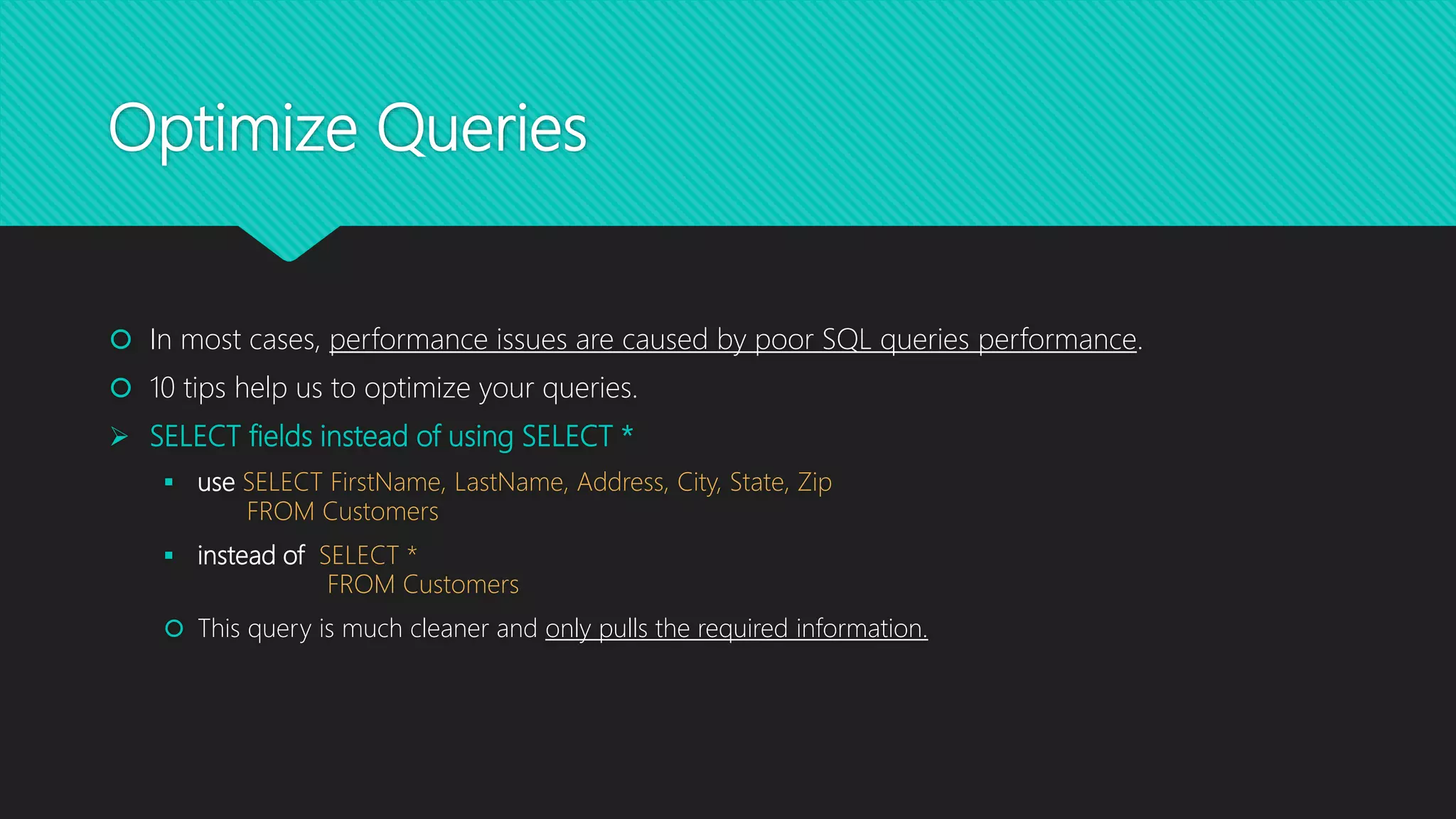
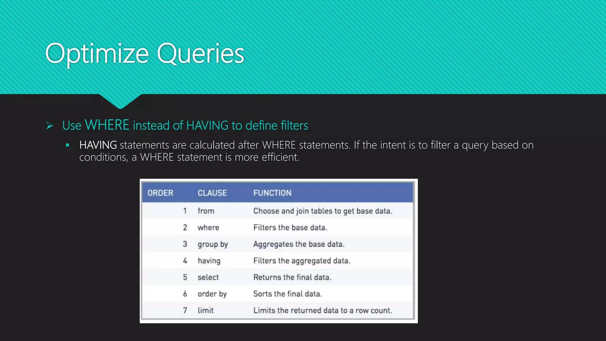
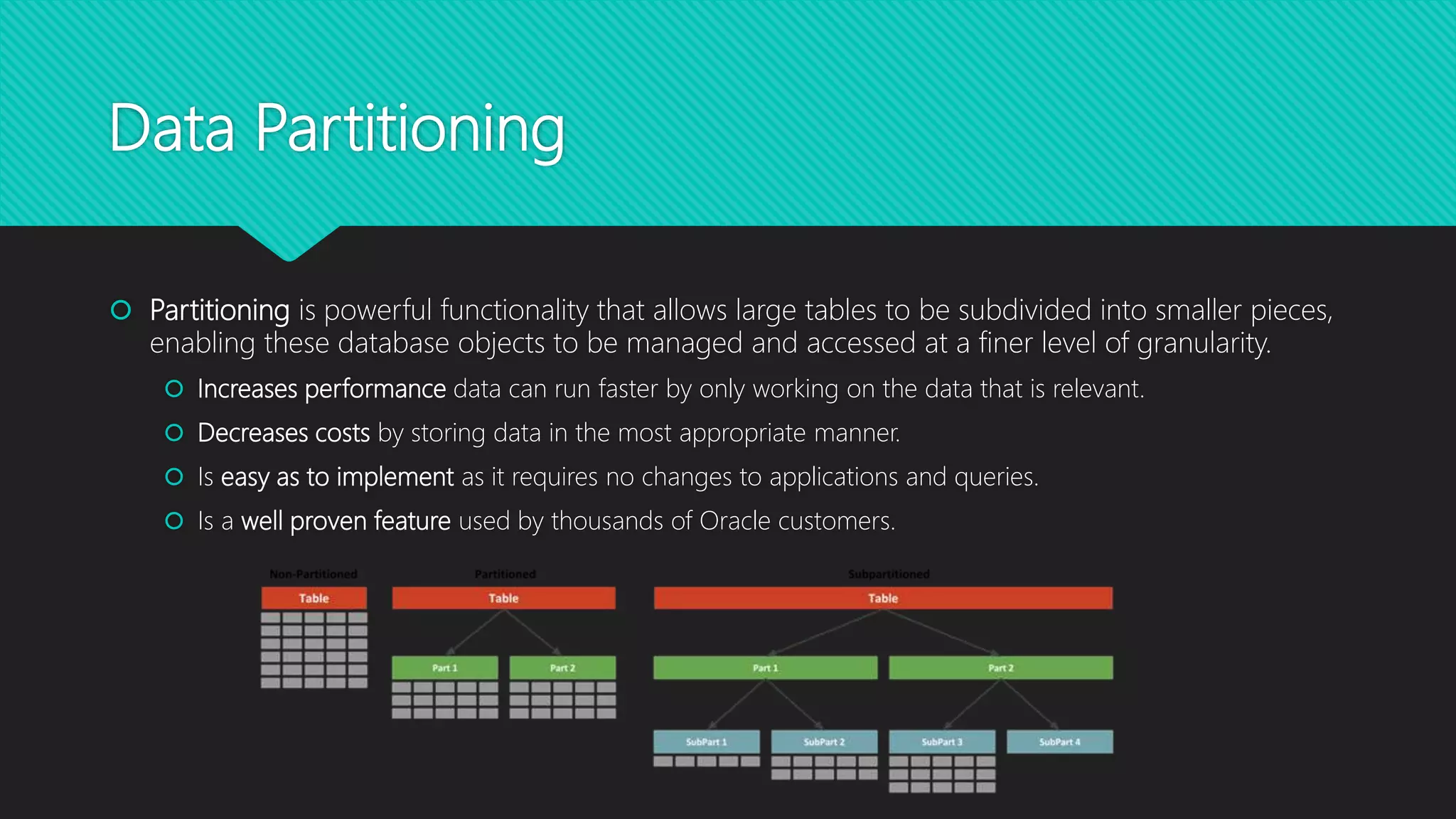
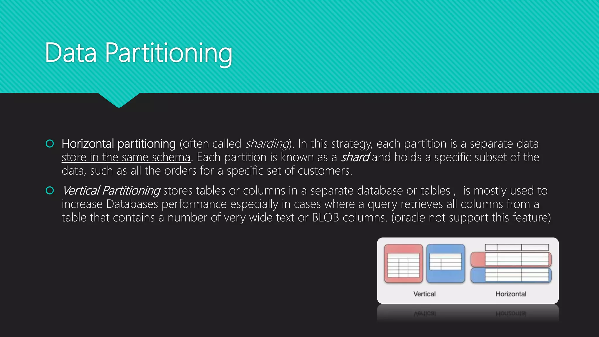
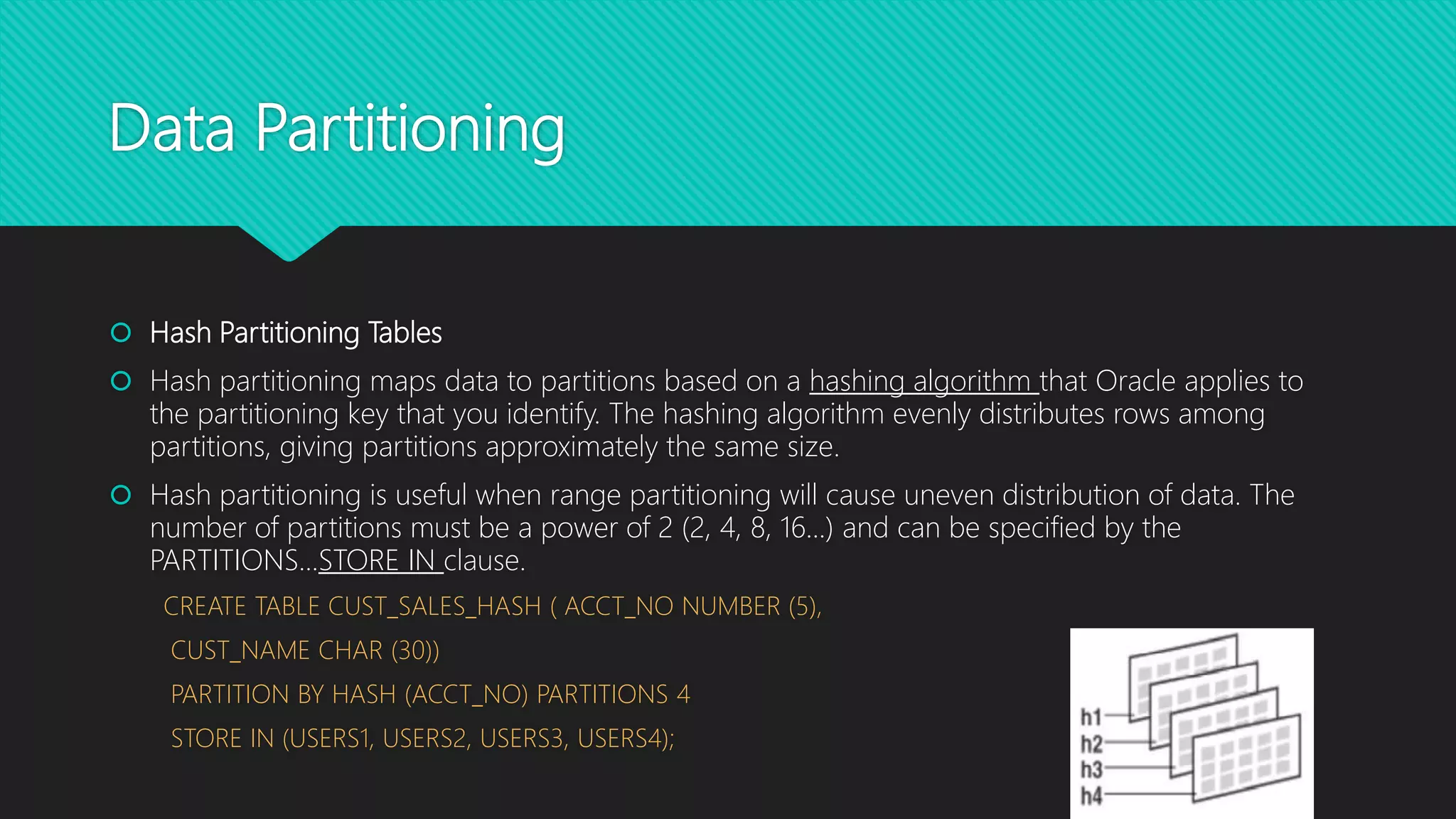
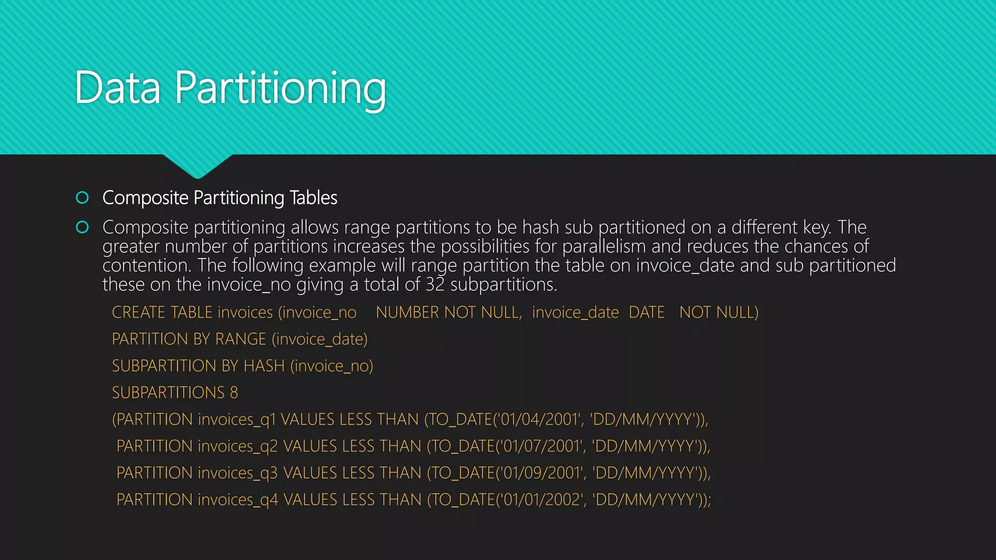
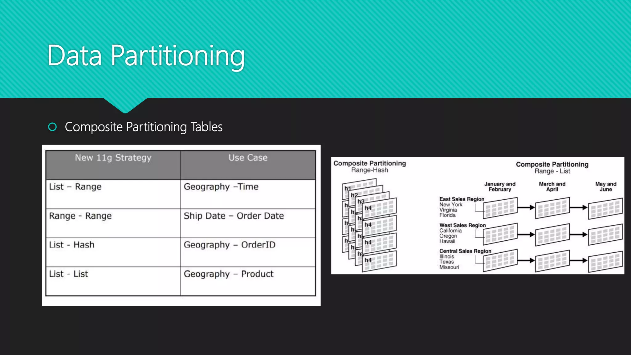
Database optimization

Database Optimization
Segmatek Co.

Improve Your Database Performance
 Get a stronger Server
 Database version
 Optimize Queries
 Create optimal indexes
 Data partitioning

Get a stronger Server
 CPU : The better your CPU, the faster and more efficient your database will be. if your database
underperforms, you should consider upgrading to a higher class CPU unit
 Disk Space :The database actually uses more disk space than they actually require. you have to
make sure that you have enough disk space available for your server. You should also run your
database on dedicated hard disks. You can deal with this by using a database caching
mechanism. It will help you in optimizing your database performance. You can also add more
hard disks for increasing your server performance.
 Memory : having more memory available will help to boost the system’s efficiency and overall
performance.

Database version
 Another major factor in database performance is the version of Database you're currently
deploying.
 Staying up to date with the latest version of your database can have significant impact on overall
database performance. It's possible that one query may perform better in older versions of
Database than in new ones, but when looking at overall performance, new versions tend to
perform better.

Optimize Queries
 In most cases, performance issues are caused by poor SQL queries performance.
 10 tips help us to optimize your queries.
 SELECT fields instead of using SELECT *
 use SELECT FirstName, LastName, Address, City, State, Zip
FROM Customers
 instead of SELECT *
FROM Customers
 This query is much cleaner and only pulls the required information.

Optimize Queries
 Avoid SELECT DISTINCT
 SELECT DISTINCT is a handy way to remove duplicates from a query. SELECT DISTINCT works
by GROUPing all fields in the query to create distinct results.
 To avoid using SELECT DISTINCT, select more fields to create unique results.
Inefficient : SELECT DISTINCT FirstName, LastName, State
FROM Customers
 This query doesn’t account for multiple people in the same state having the same first and last name.
Popular names such as David Smith or Diane Johnson will be grouped together, causing an inaccurate
number of records. In larger databases, a large number of David Smiths and Diane Johnsons will cause
this query to run slowly.
Efficient : SELECT FirstName, LastName, Address, City, State, ZipCode
FROM Customers
 By adding more fields, unduplicated records were returned without using SELECT DISTINCT. The
database does not have to group any fields, and the number of records is accurate.

Optimize Queries
 Create joins with INNER JOIN (not WHERE)
 Some SQL developers prefer to make joins with WHERE clauses, such as the following:
SELECT Customers.CustomerID, Customers.Name, Sales.LastSaleDate
FROM Customers, Sales
WHERE Customers.CustomerID = Sales.CustomerID
 This type of join creates a Cartesian Join, also called a Cartesian Product or CROSS JOIN.
 In a Cartesian Join, all possible combinations of the variables are created. In this example, if we had 1,000
customers with 1,000 total sales, the query would first generate 1,000,000 results (all possible combinations), then
filter for the 1,000 records where CustomerID is correctly joined.
 To prevent creating a Cartesian Join, use INNER JOIN instead:
SELECT Customers.CustomerID, Customers.Name, Sales.LastSaleDate
FROM Customers
INNER JOIN Sales
ON Customers.CustomerID = Sales.CustomerID
The database would only generate the 1,000 desired records where CustomerID is equal.
 Some DBMS systems are able to recognize WHERE joins and automatically run them as INNER JOINs instead. In
those DBMS systems, there will be no difference in performance between a WHERE join and INNER JOIN.

Optimize Queries
 Use WHERE instead of HAVING to define filters
 HAVING statements are calculated after WHERE statements. If the intent is to filter a query based on
conditions, a WHERE statement is more efficient.

Optimize Queries
 let’s assume 200 sales have been made in the year 2016, and we want to query for the number of sales
per customer in 2016.
SELECT Customers.CustomerID, Customers.Name, Count(Sales.SalesID)
FROM Customers
INNER JOIN Sales
GROUP BY Customers.CustomerID, Customers.Name
HAVING Sales.LastSaleDate BETWEEN #1/1/2016# AND #12/31/2016#
 This query would pull 1,000 sales records from the Sales table, then filter for the 200 records generated
in the year 2016, and finally count the records in the dataset.

Optimize Queries
FROM Customers
INNER JOIN Sales
WHERE Sales.LastSaleDate BETWEEN #1/1/2016# AND #12/31/2016#
 This query would pull the 200 records from the year 2016, and then count the records in the dataset. The first
step in the HAVING clause has been completely eliminated.
 HAVING should only be used when filtering on an aggregated field. In the query above, we could
additionally filter for customers with greater than 5 sales using a HAVING statement.
FROM Customers
INNER JOIN Sales
HAVING Count(Sales.SalesID) > 5

Optimize Queries
 Use wildcards at the end of a phrase only
 When searching plaintext data, such as cities or names, wildcards create the widest search
possible. However, the widest search is also the most inefficient search.
 Consider this query to pull cities beginning with ‘Char’:
SELECT City FROM Customers
WHERE City LIKE ‘%Char%’
This query will pull the expected results of Charleston, Charlotte, and Charlton. However, it will also pull
unexpected results, such as Cape Charles, Crab Orchard, and Richardson.
 A more efficient query would be:
SELECT City FROM Customers
WHERE City LIKE ‘Char%’
This query will pull only the expected results of Charleston, Charlotte, and Charlton.

Optimize Queries
 Use LIMIT to sample query results
 Before running a query for the first time, ensure the results will be desirable and meaningful by
using a LIMIT statement. (In some DBMS systems, the word TOP is used interchangeably with
LIMIT.) The LIMIT statement returns only the number of records specified.
 In the 2016 sales query from above, we will examine a limit of 10 records:
FROM Customers
INNER JOIN Sales
LIMIT 10

Optimize Queries
 Run your query during off-peak hours
 In order to minimize the impact of your analytical queries on the production database, talk to a
DBA(database administrator) about scheduling the query to run at an off-peak time. The query
should run when concurrent users are at their lowest number, which is typically the middle of
the night (3 – 5 a.m.) ,The more of the following criteria your query has, the more likely of a
candidate it should be to run at night:
 Selecting from large tables (>1,000,000 records)
 Cartesian Joins or CROSS JOINs
 Looping statements
 SELECT DISTINCT statements
 Nested subqueries
 Wildcard searches in long text or memo fields
 Multiple schema queries

Optimize Queries
 Run DELETE and UPDATE Queries in Batches
 Deleting and updating data — especially in very large tables — can be complicated. It can take
a lot of time and both these commands are executed as a single transaction. This means that in
case of any interruptions, the entire transaction must be rolled back, which can be even more
time-consuming.
 However, if you follow the good practice of running DELETE and UPDATE queries in batches,
you will be able to save time by increasing concurrency and reducing bottlenecks.
 If you delete and update a smaller number of rows at a time, other queries can be executed
when the batches are being committed to the disk. And any roll-backs that you might have to
do will take less time.

Optimize Queries
 Keep Your Tables Static (Fixed-length)
 Another great way to optimize your database performance is to use static tables.
 This means that your table shouldn’t include any columns with variable lengths, like TEXT or
BLOB. You can use CHAR, VARCHAR, BINARY, and VARBINARY columns, but they need to be
padded so that they match the specified column width.
 Using fixed-length tables is beneficial as they are faster and easier to cache. In addition to that,
static tables are more secure — they’re easier to reconstruct after a crash.
 Use EXPLAIN with Your SELECT Queries
 Using the EXPLAIN keyword is a great way to quickly fix slow queries. It gives you insight into
how your query will be carried out and help you find potential places for query optimization.
 Simply type the EXPLAIN keyword in front of your SELECT query. This won’t trigger the actual
query, but instead, you will see the execution plan.

Create Optimal Indexes
What is Index ? A database index allows a query to efficiently retrieve data from a database. Indexes are
related to specific tables and consist of one or more keys. A table can have more than one index built
from it. use INDEX to avoid scan all the table
 A book has a table of contents. When searching for a topic in the book, we can quickly find out the
page number of the topic we’re looking for from the table of contents.
Indexing is a data structure technique which allows you to quickly retrieve records from a database file. An
Index is a small table having only two columns. The first column comprises a copy of the primary key of a
table. Its second column contains a set of pointers for holding the address of the disk block where that
specific key value stored.
An index :
 Takes a search key as input
 Efficiently returns a collection of matching records.

 Consider the following list of indexing design ideas when building a new index:
 Using a Different Index Type : There are several index types available, and each index has benefits
for certain situations. The following list gives performance ideas associated with each index type.
 B-Tree Indexes : These indexes are the standard index type, and they are excellent for primary
key and highly-selective indexes. the database can use B-tree indexes to retrieve data sorted by
the index columns.
CREATE INDEX name_of_index
ON table_name(column);

 The B-tree index is similar to the tree structure
 When Database wants to access the index, it starts with the outermost root block. The root level
determines the second level of the branch block. Branch block leads to what we call leaf.
 This leaf block has the ROWID information required for us
 After reaching the ROWID information readings to access the ROWID information, it will now
read the block containing the relevant ROWID information in our table.

 Bitmap Index: This index type is the most commonly used index type after B-Tree. Bitmap
Indexing is a special type of database indexing that uses bitmaps technique is used for huge
databases, when column is of low cardinality (indexes with relatively few unique values) and these
columns are most used in the query.
 Bit: Bit is a basic unit of information used in computing that can have only one of two values
either 0 or 1 (true or false).
 For example, there are only 2 values for the Gender Column. This value is repeated for each user,
male and female, or columns where a limited number of values can be entered, such as Yes or
No or any unique values.
 CREATE BITMAP INDEX Index_Name ON Table_Name (Column_Name);

SELECT * FROM STUDENT WHERE New_Emp = "No" and
Job = "Salesperson";
Here the result 0100 represents that the second column
has to be retrieved as a result.
Now Suppose, If we want to find out the details for the
Employee who is not new in the company and is a sales
person then we will run the query:
Employee example, Given below is the Employee table :

 Function-Based Index: In this type of index, When you use the function in the Where condition of
your queries, it will not use the index unless you have created the index with this function. In this
case you need to create Function based index . An example of this and the corresponding script
is as follows.
Create index MAD_IX on customer (lower(name));
When you create an Function based index like above, the query will use the index despite the lower
function put in the where condition.

 Concatenated Index: This type of index is actually the advanced version of the B-Tree index. With
Concatenated Index we can concatenate more than one column in an index.(We can create
indexes on multiple columns. Multiple column indexes created in this way are called
Concatenated Index.) For example: In the Customer Table, we can index and query the Name
and Surname column.
Create index MAD_IX on customer(name,lastname);
When creating an index as above, the following query will be able to use the index.
select * from customer where name='mehmet' and lastname='deveci';
 Unique Index: This type of index is the advanced version of the B-Tree index structure. Normally,
the B-Tree index structure is Non-Unique. When we use the Unique keyword to create this index
type, Oracle will create a Unique index. This type of index is especially used on columns with
unique records. It is created as follows.
Create unique index MTC_IX on customer(SSID);

 Reverse Key Index: A Reverse Key Index simply takes the index column values and reverses them
before inserting into the index. This index is an improved type of B-Tree index. In this index type,
the value of the index key is always reversed. Ex; Suppose that our index values are 123, 456, 789,
in this case Reversed key index values will be 321, 654, 987. This index is created as follows.
create Index MID_IX on customer(customer_id) reverse;
 Compressed Index : The use of index compression in indexes with multiple columns can be very
useful, especially if the column contains data repetition.
 Compress : Oracle 9i onward allows whole tables or individual table partitions to be compressed to
reduce disk space requirements.
Less disk space and less I / O operation to achieve compressed index.
CREATE INDEX INDX_COMP ON HR.EMPLOYEES (FIRST_NAME, LAST_NAME) COMPRESS 2;

 Invisible Index : One of the features that come with 11g. Invisible indexes are not visible by Oracle
optimizer.
 Especially useful when testing the effect of the index on our queries. We can make the index
invisible at any time and make it visible at any time. If an index is invisible and made visible again,
the index does not need to be rebuilt
 When an index is disabled with UNUSABLE, the index must be rebuilt before it can be reused.
This process takes time.
 ALTER INDEX INDX_1 INVISIBLE;
 ALTER INDEX INDX_1 VISIBLE;

Data Partitioning
 Partitioning is powerful functionality that allows large tables to be subdivided into smaller pieces,
enabling these database objects to be managed and accessed at a finer level of granularity.
 Increases performance data can run faster by only working on the data that is relevant.
 Decreases costs by storing data in the most appropriate manner.
 Is easy as to implement as it requires no changes to applications and queries.
 Is a well proven feature used by thousands of Oracle customers.

Data Partitioning
 Horizontal partitioning (often called sharding). In this strategy, each partition is a separate data
store in the same schema. Each partition is known as a shard and holds a specific subset of the
data, such as all the orders for a specific set of customers.
 Vertical Partitioning stores tables or columns in a separate database or tables , is mostly used to
increase Databases performance especially in cases where a query retrieves all columns from a
table that contains a number of very wide text or BLOB columns. (oracle not support this feature)

Data Partitioning
 Partitioning Types in oracle:
 Range Partitioning
 List Partitioning
 Auto-List Partitioning
 Hash Partitioning .
 Composite Partitioning
 Interval Partitioning
 Multi-Column Range Partitioning
 Reference Partitioning Partitions
 Virtual Column Based Partitioning
 Interval Reference Partitioning

Data Partitioning
 Partition key : column that will partitioning the table with.
 Range Partitioning Tables
 Range partitioning is useful when you have distinct ranges of data you want to store together. The
classic example of this is the use of dates. Partitioning a table using date ranges allows all data of a
similar age to be stored in same partition. Once historical data is no longer needed the whole partition
can be removed. If the table is indexed correctly search criteria can limit the search to the partitions
that hold data of a correct age.
CREATE TABLE invoices (invoice_no NUMBER NOT NULL, invoice_date DATE NOT NULL)
PARTITION BY RANGE (invoice_date)
(PARTITION invoices_q1 VALUES LESS THAN (TO_DATE('01/04/2001', 'DD/MM/YYYY')) TABLESPACE users,
PARTITION invoices_q2 VALUES LESS THAN (TO_DATE('01/07/2001', 'DD/MM/YYYY')) TABLESPACE users,
PARTITION invoices_q3 VALUES LESS THAN (TO_DATE('01/09/2001', 'DD/MM/YYYY')) TABLESPACE users;

Data Partitioning
 List Partitioning The data distribution is defined by a discrete list of values. One or multiple
columns can be used as partition key.
CREATE TABLE sales_by_region (item# INTEGER, qty INTEGER, store_name VARCHAR(30), state_code
VARCHAR(2), sale_date DATE)
PARTITION BY LIST (state_code) (
PARTITION region_east
VALUES ('MA','NY','CT','NH','ME','MD','VA','PA','NJ')
PARTITION region_west
VALUES ('CA','AZ','NM','OR','WA','UT','NV','CO')
PARTITION region_south
VALUES ('TX','KY','TN','LA','MS','AR','AL','GA'));

Data Partitioning
 Hash Partitioning Tables
 Hash partitioning maps data to partitions based on a hashing algorithm that Oracle applies to
the partitioning key that you identify. The hashing algorithm evenly distributes rows among
partitions, giving partitions approximately the same size.
 Hash partitioning is useful when range partitioning will cause uneven distribution of data. The
number of partitions must be a power of 2 (2, 4, 8, 16...) and can be specified by the
PARTITIONS...STORE IN clause.
CREATE TABLE CUST_SALES_HASH ( ACCT_NO NUMBER (5),
CUST_NAME CHAR (30))
PARTITION BY HASH (ACCT_NO) PARTITIONS 4
STORE IN (USERS1, USERS2, USERS3, USERS4);

Data Partitioning
 Composite Partitioning Tables
 Composite partitioning allows range partitions to be hash sub partitioned on a different key. The
greater number of partitions increases the possibilities for parallelism and reduces the chances of
contention. The following example will range partition the table on invoice_date and sub partitioned
these on the invoice_no giving a total of 32 subpartitions.
CREATE TABLE invoices (invoice_no NUMBER NOT NULL, invoice_date DATE NOT NULL)
PARTITION BY RANGE (invoice_date)
SUBPARTITION BY HASH (invoice_no)
SUBPARTITIONS 8
(PARTITION invoices_q1 VALUES LESS THAN (TO_DATE('01/04/2001', 'DD/MM/YYYY')),
PARTITION invoices_q2 VALUES LESS THAN (TO_DATE('01/07/2001', 'DD/MM/YYYY')),
PARTITION invoices_q3 VALUES LESS THAN (TO_DATE('01/09/2001', 'DD/MM/YYYY')),
PARTITION invoices_q4 VALUES LESS THAN (TO_DATE('01/01/2002', 'DD/MM/YYYY'));

Data Partitioning
 Composite Partitioning Tables

Data Partitioning
 Interval Partitioning - Interval Partitioning has been introduced in oracle 11g. we can automate the
creation of range partition .While creating the partitioned table, we just need to define one partition. New
partitions will be created automatically based on interval criteria when the data is inserted to the table. We
don’t need to create the future partitions.
 Auto-List Partitioning - Auto-List Partitioning was introduced with Oracle 12c Release 2 and is an extension
of LIST Partitioning. Similar to INTERVAL Partitioning, new partitions can now be created automatically
when new rows are inserted into a LIST partitioned table.
 Reference Partitioning Partitions - an existing parent-child relationship. The primary key relationship is used
to inherit the partitioning strategy of the parent table to its child table.
 Virtual Column Based Partitioning - allows the partitioning key to be an expression, using one or more
existing columns of a table, and storing the expression as metadata only.
 Multi-Column Range Partitioning - allows us to specify more than one column as a partition key.
 Interval Reference Partitioning - an extension to reference partitioning that allows the use of interval
partitioned tables as parent tables for reference partitioning.
 Partitioning Existing Tables - The ALTER TABLE ... EXCHANGE PARTITION ... syntax can be used to partition
an existing table.

Database optimization

More Related Content

Similar to Database optimization

Recently uploaded

Database optimization