CS8451 - Design and Analysis of Algorithms

Mathematical analysis for
Recursive algorithms
Dr.K.Muthumanickam
Associate Professor/IT
Kongunadu College of Engineering and Technology
Tholur Patti, Thottiam Taluk
Trichy District – 621215, Tamilnadu

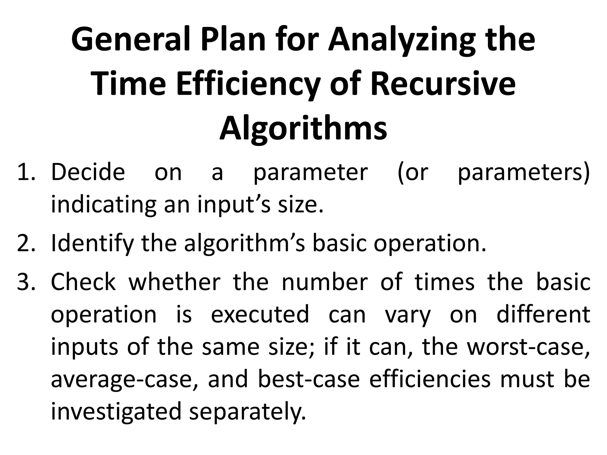
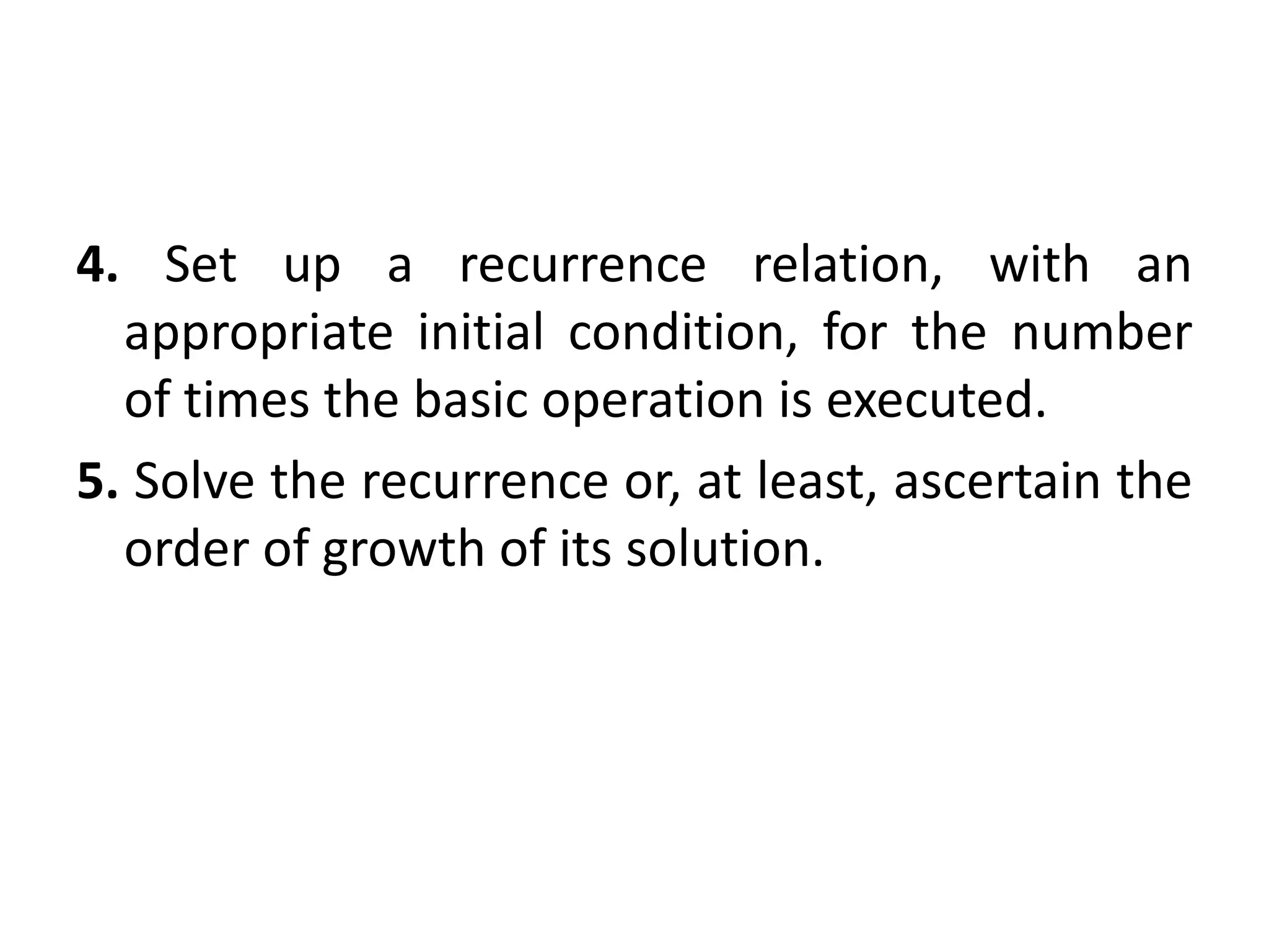
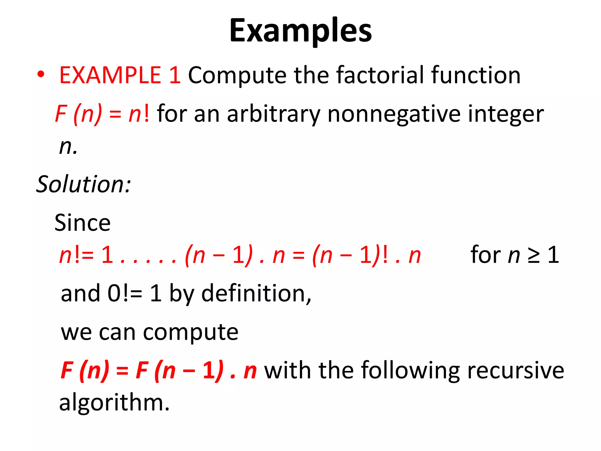
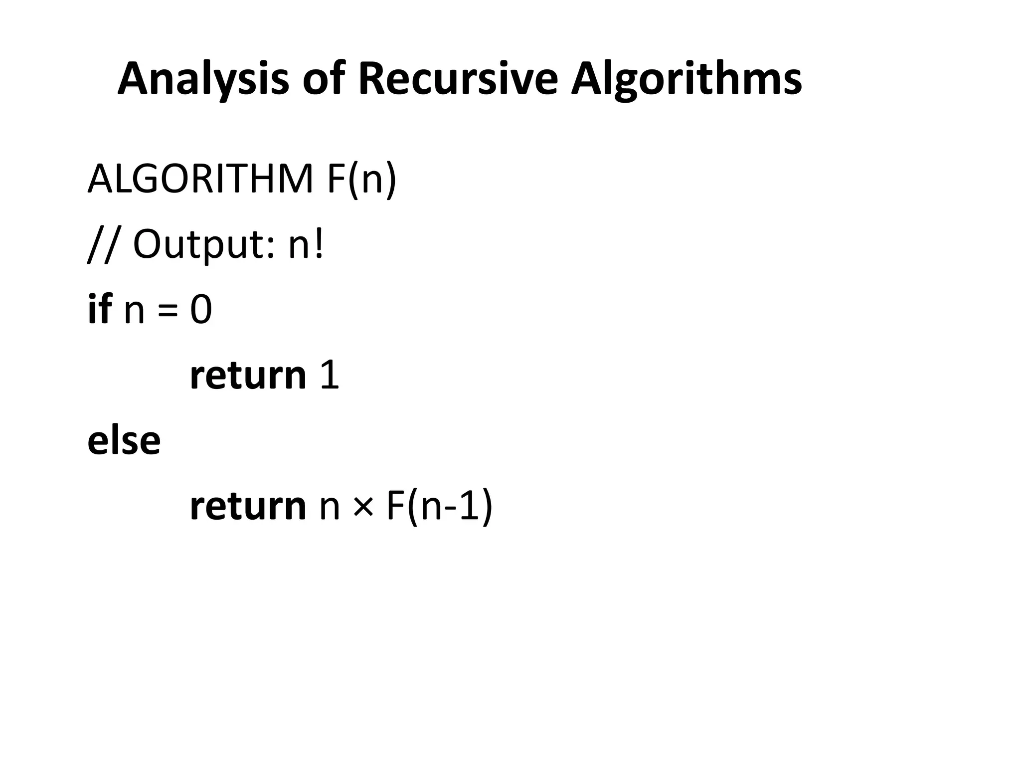
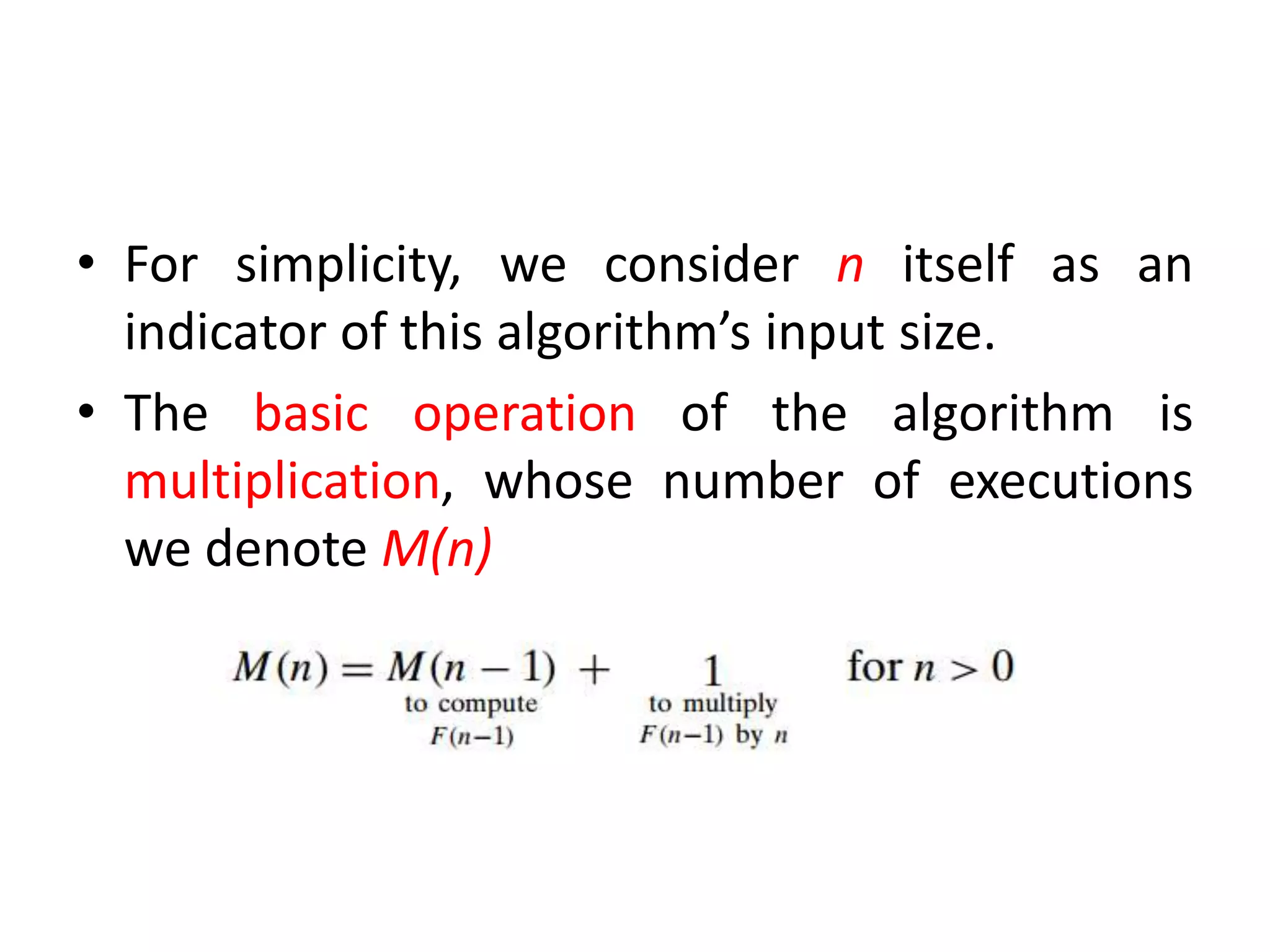
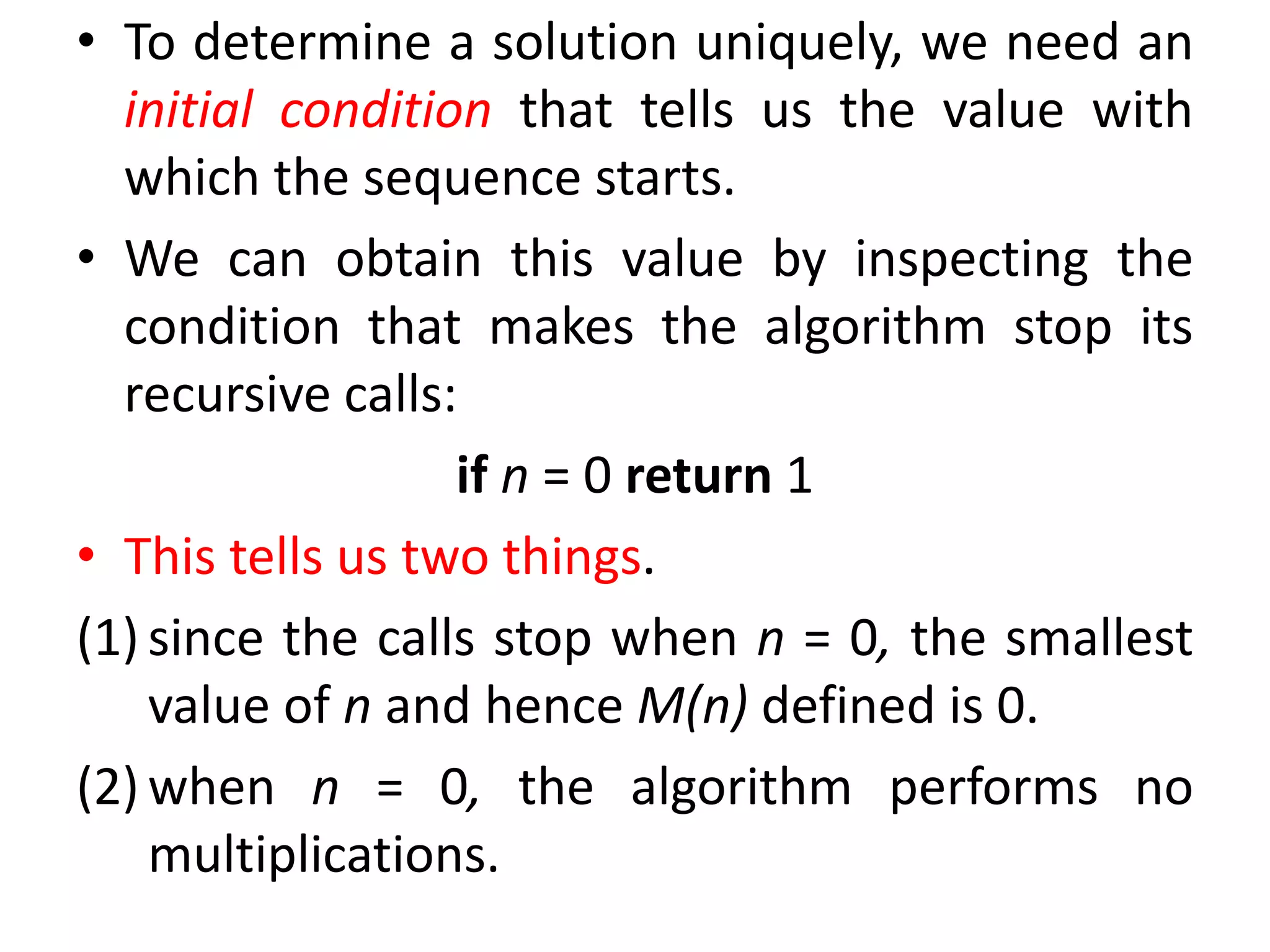
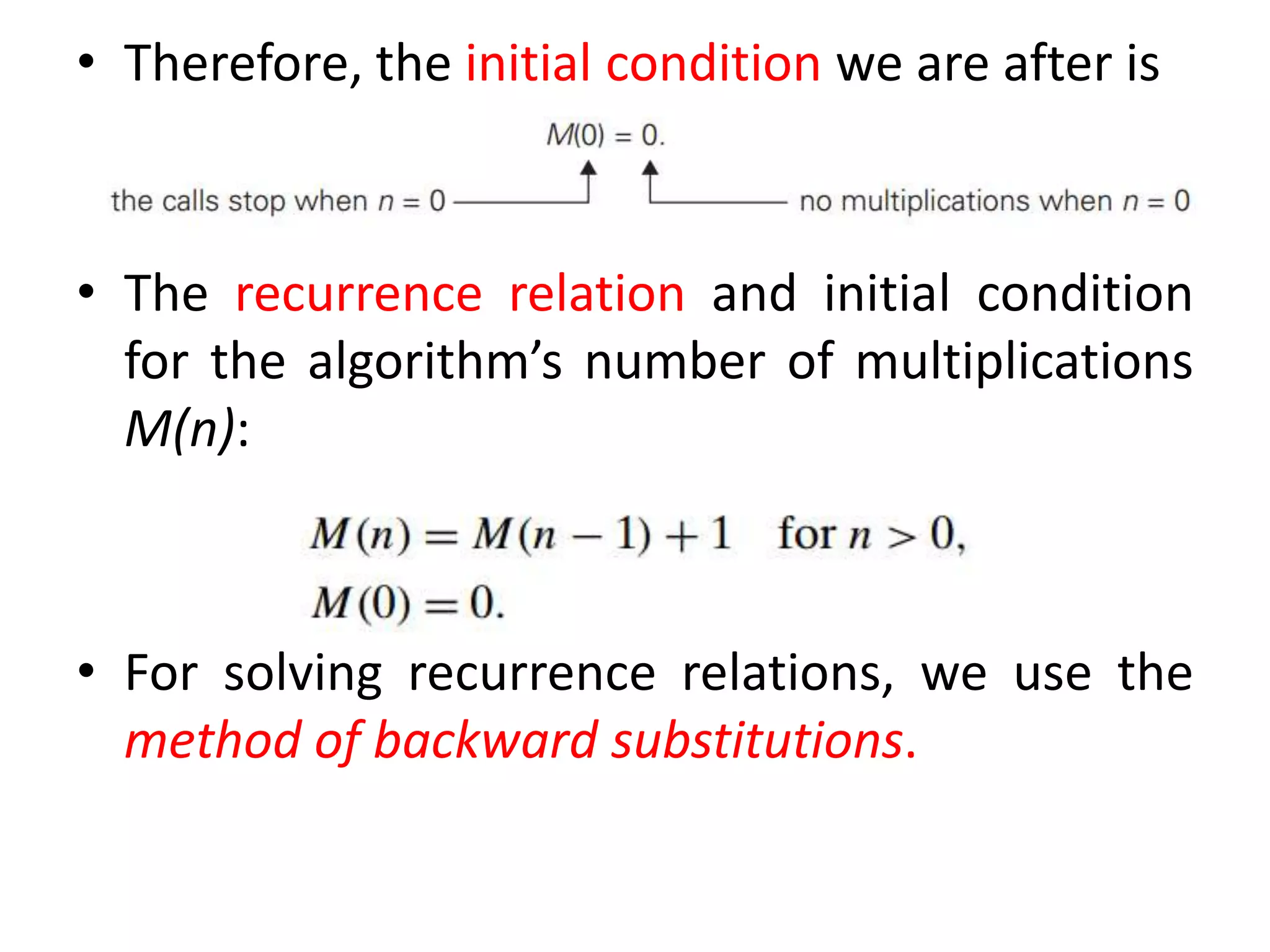
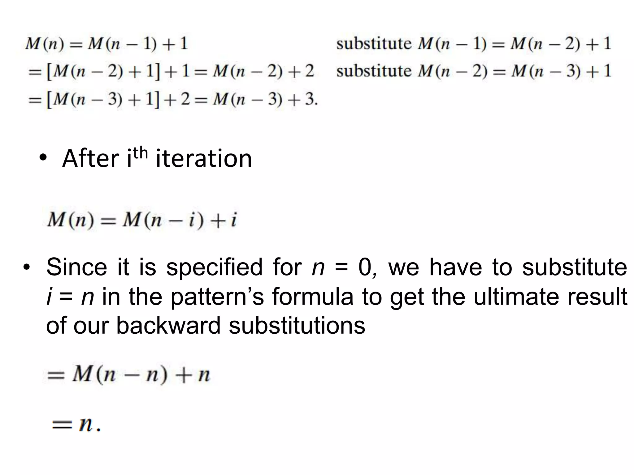
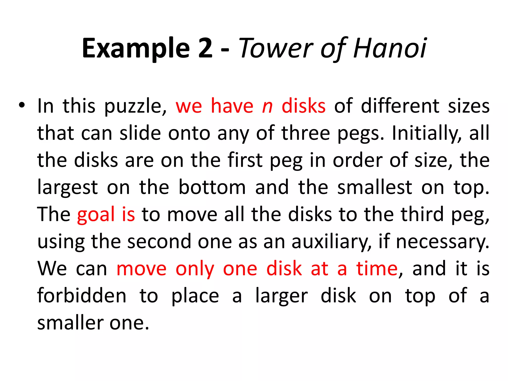
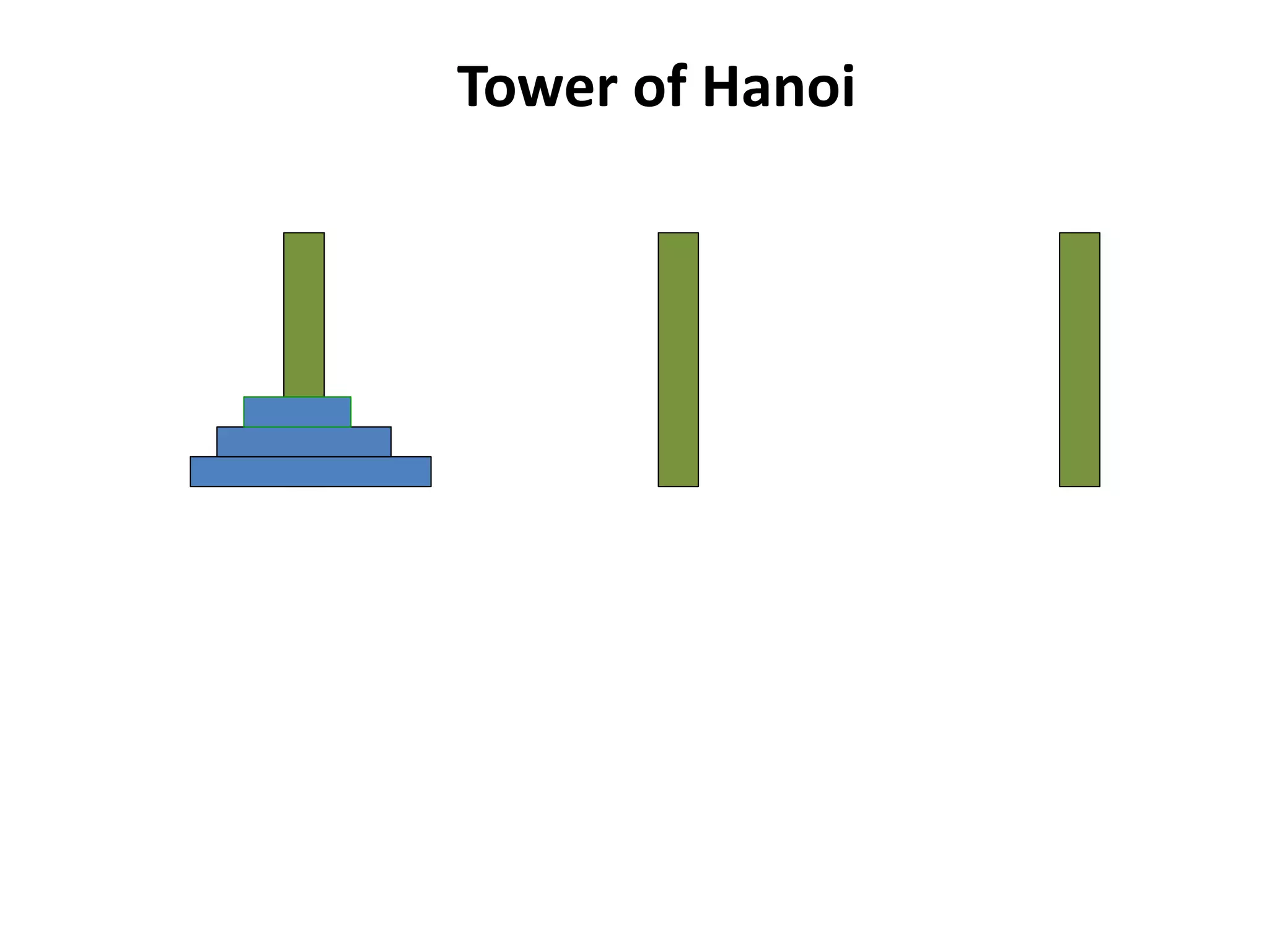
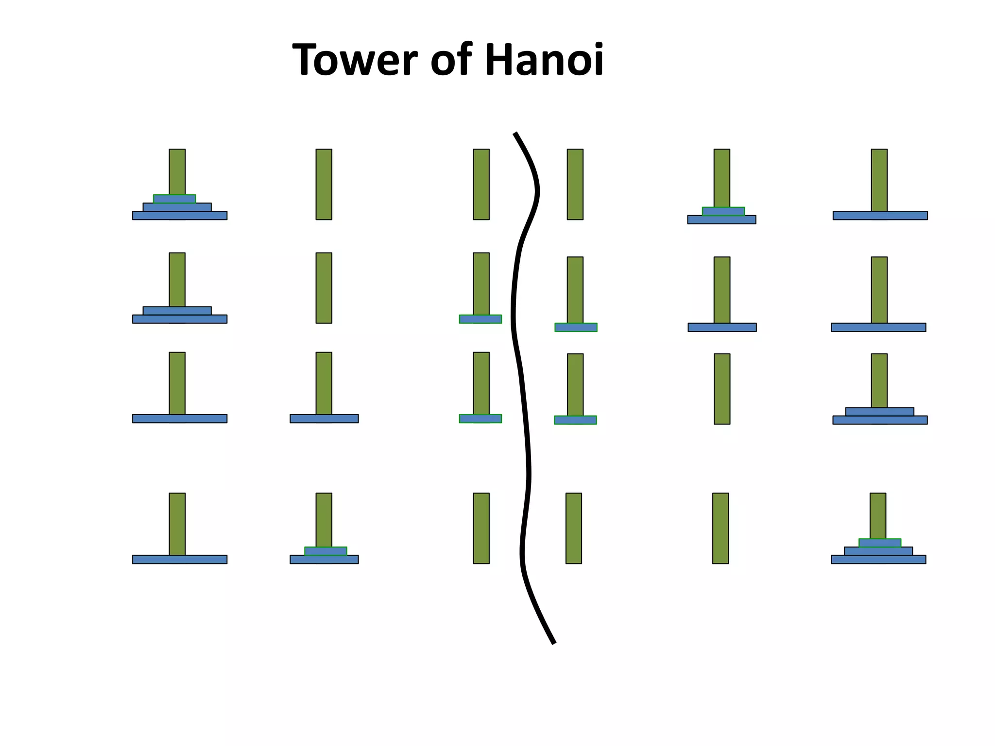
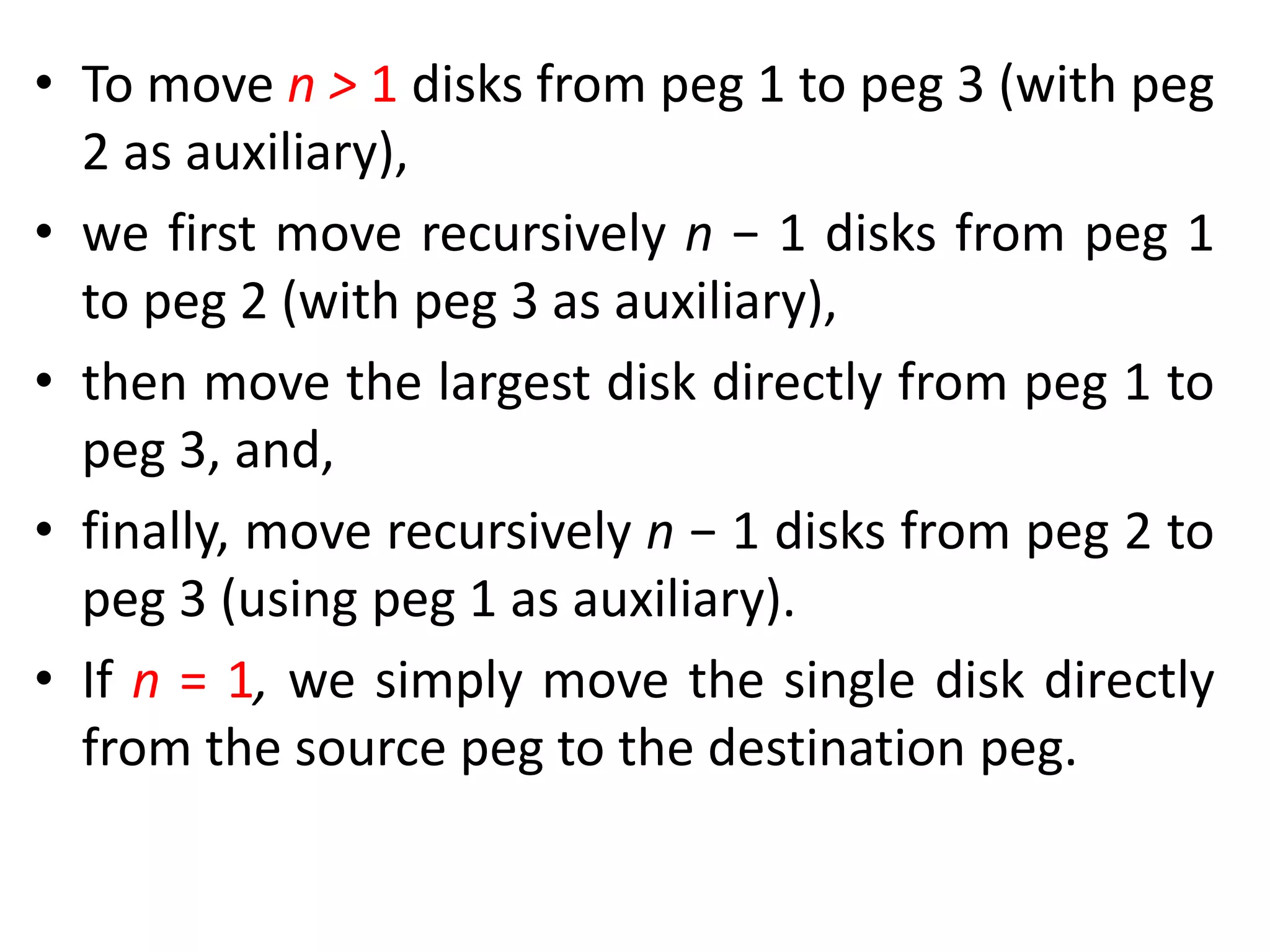
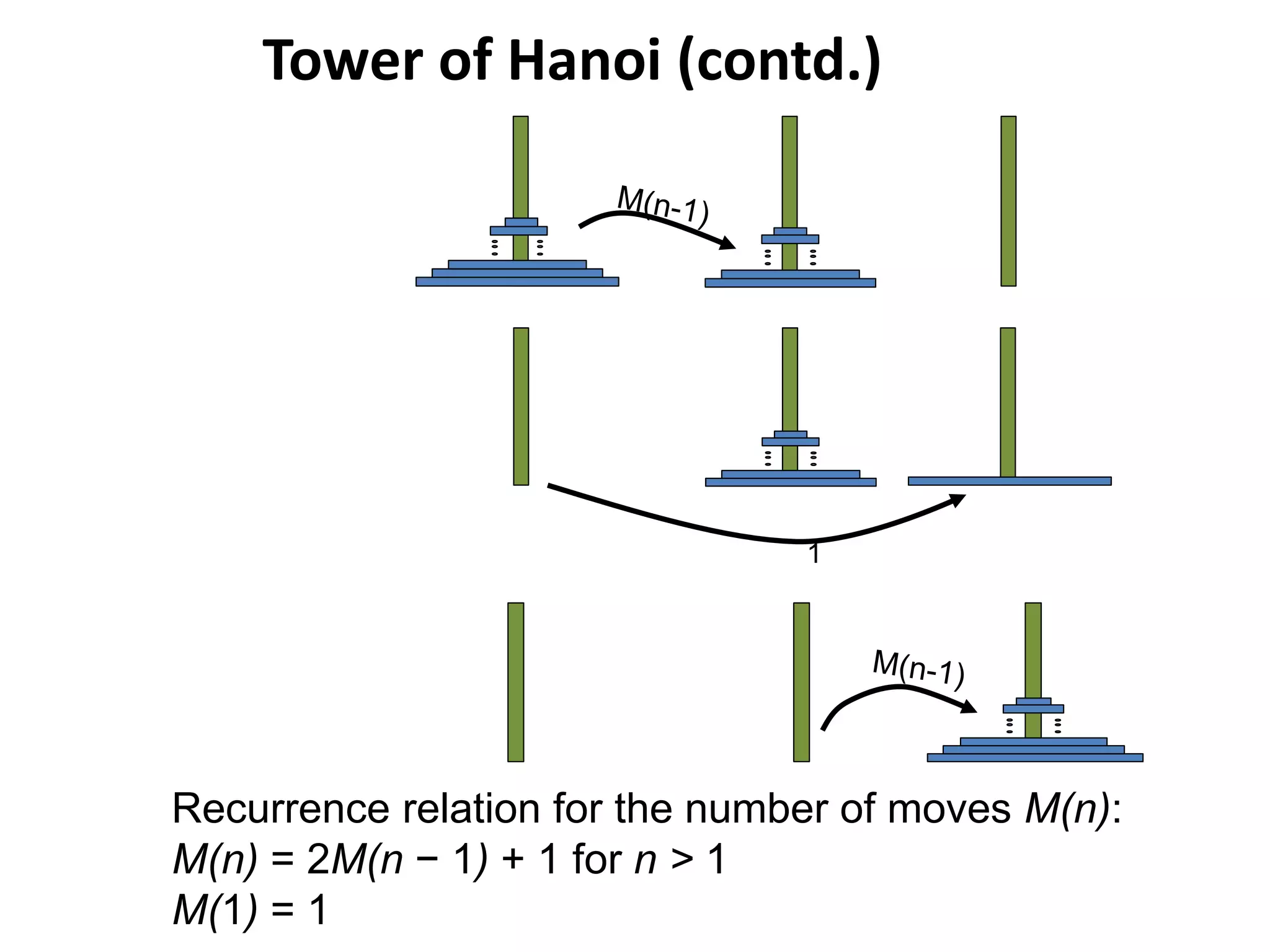
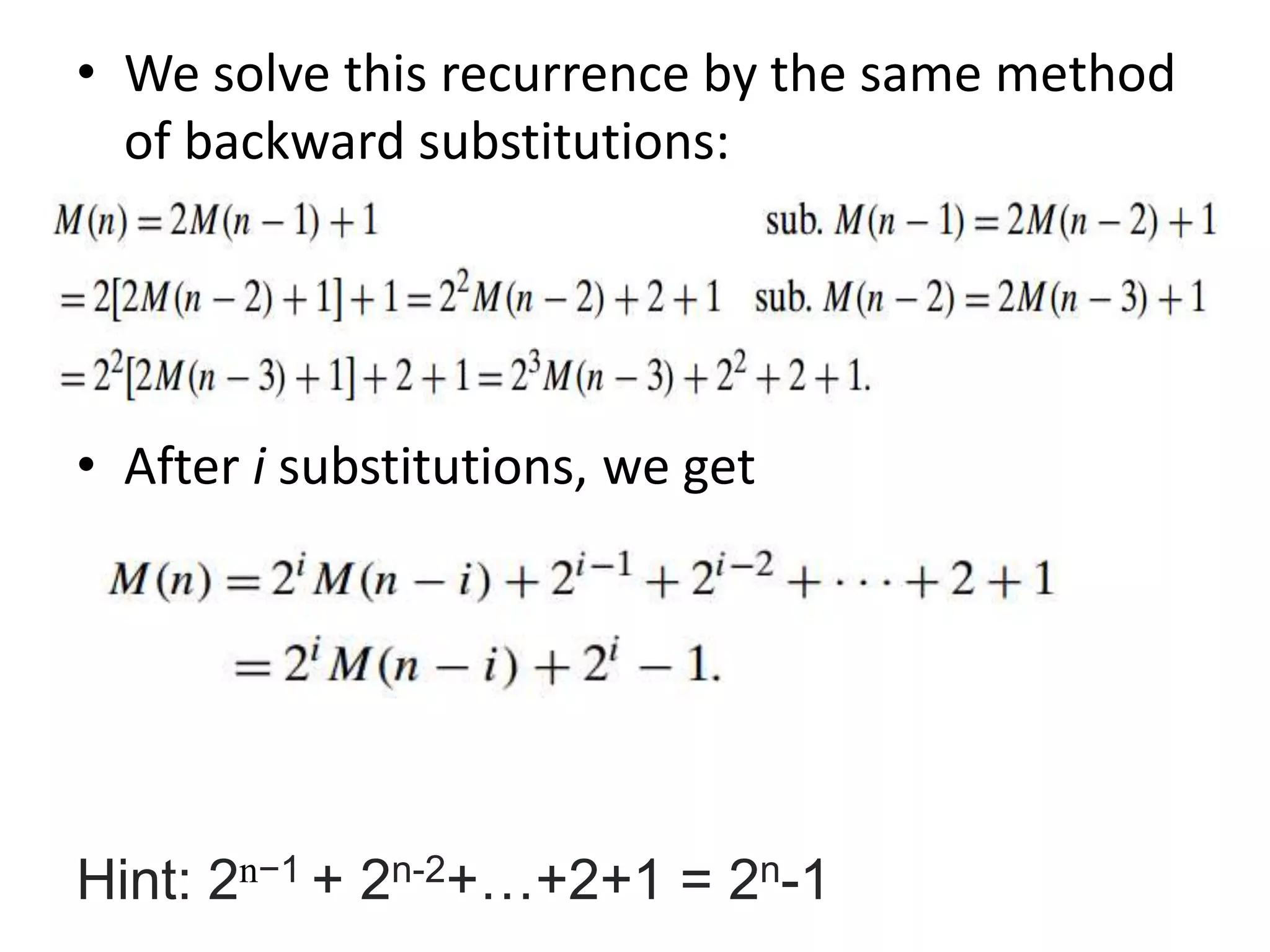
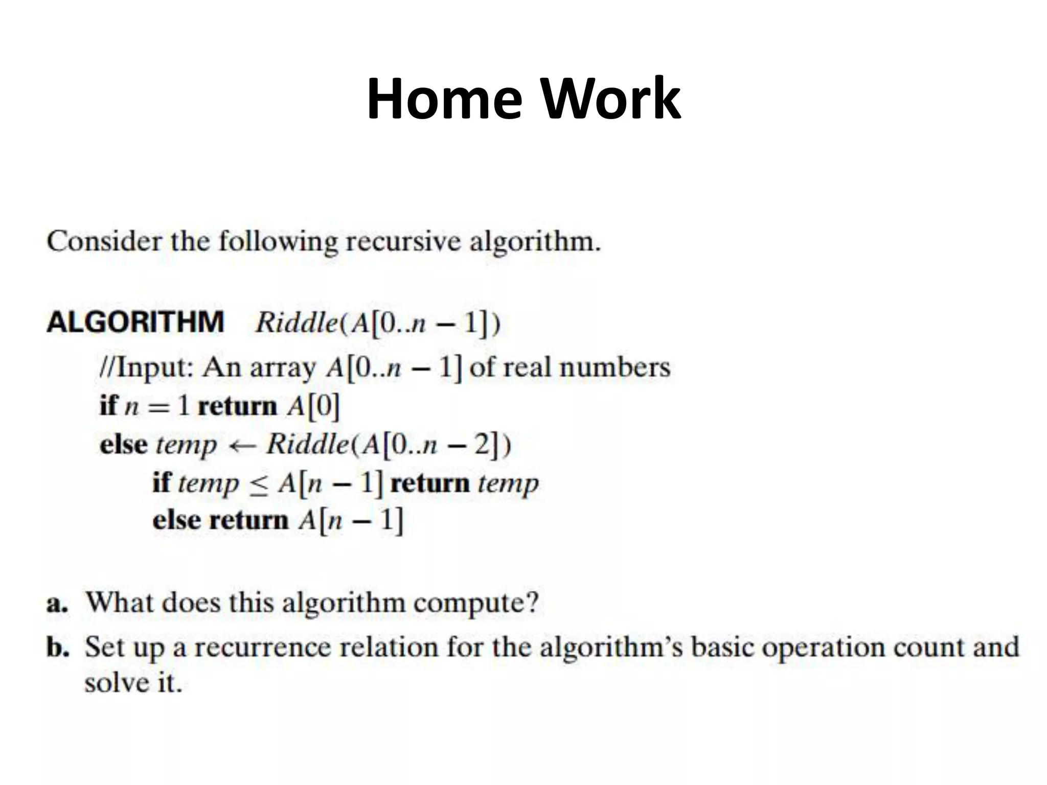
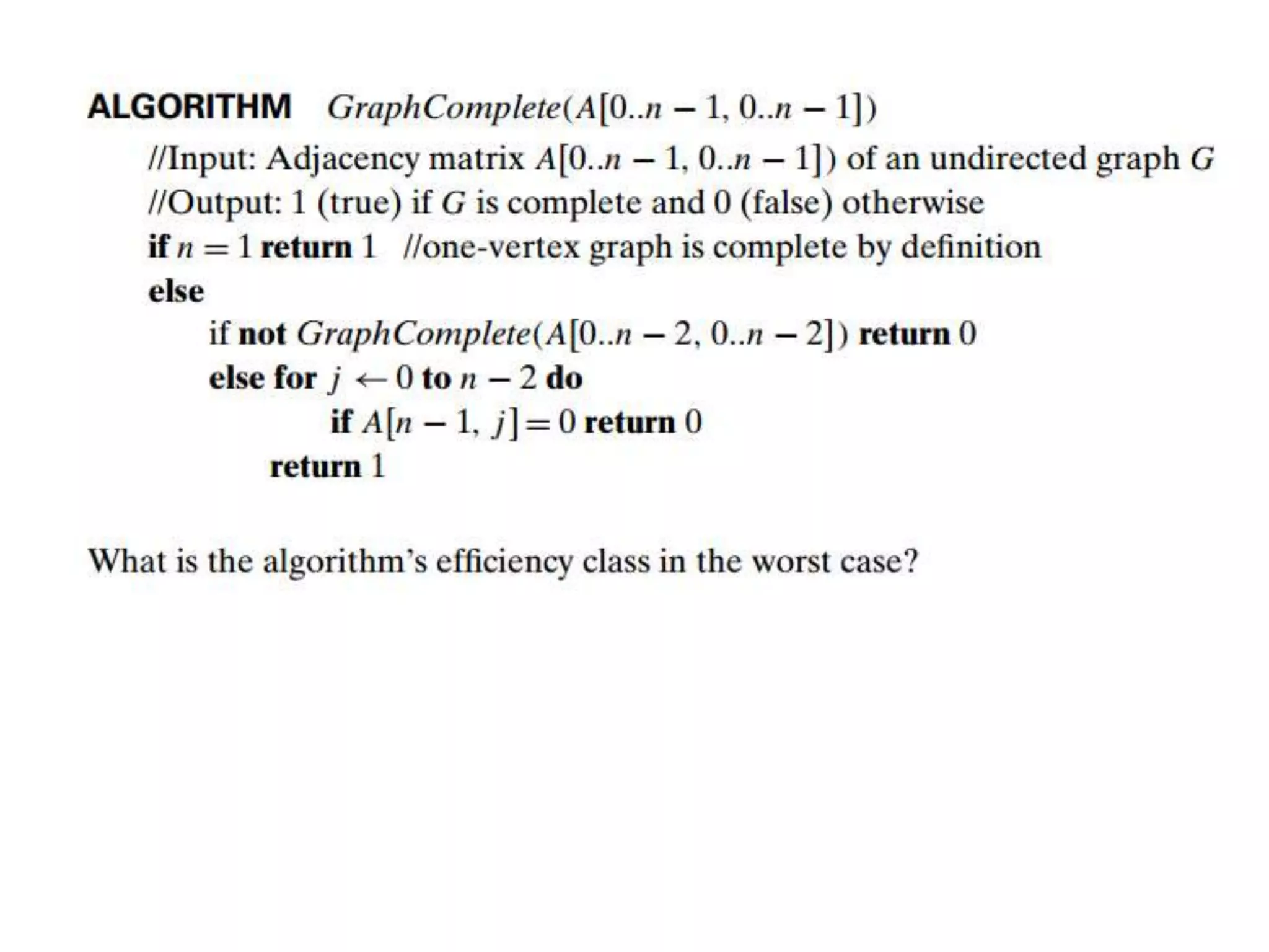
General Plan for Analyzing the
Time Efficiency of Recursive
Algorithms
1. Decide on a parameter (or parameters)
indicating an input’s size.
2. Identify the algorithm’s basic operation.
3. Check whether the number of times the basic
operation is executed can vary on different
inputs of the same size; if it can, the worst-case,
average-case, and best-case efficiencies must be
investigated separately.

4. Set up a recurrence relation, with an
appropriate initial condition, for the number
of times the basic operation is executed.
5. Solve the recurrence or, at least, ascertain the
order of growth of its solution.

Examples
• EXAMPLE 1 Compute the factorial function
F (n) = n! for an arbitrary nonnegative integer
n.
Solution:
Since
n!= 1 . . . . . (n − 1) . n = (n − 1)! . n for n ≥ 1
and 0!= 1 by definition,
we can compute
F (n) = F (n − 1) . n with the following recursive
algorithm.

Analysis of Recursive Algorithms
ALGORITHM F(n)
// Output: n!
if n = 0
return 1
else
return n × F(n-1)

• For simplicity, we consider n itself as an
indicator of this algorithm’s input size.
• The basic operation of the algorithm is
multiplication, whose number of executions
we denote M(n)

• To determine a solution uniquely, we need an
initial condition that tells us the value with
which the sequence starts.
• We can obtain this value by inspecting the
condition that makes the algorithm stop its
recursive calls:
if n = 0 return 1
• This tells us two things.
(1) since the calls stop when n = 0, the smallest
value of n and hence M(n) defined is 0.
(2) when n = 0, the algorithm performs no
multiplications.

• Therefore, the initial condition we are after is
• The recurrence relation and initial condition
for the algorithm’s number of multiplications
M(n):
• For solving recurrence relations, we use the
method of backward substitutions.

• After ith iteration
• Since it is specified for n = 0, we have to substitute
i = n in the pattern’s formula to get the ultimate result
of our backward substitutions

Example 2 - Tower of Hanoi
• In this puzzle, we have n disks of different sizes
that can slide onto any of three pegs. Initially, all
the disks are on the first peg in order of size, the
largest on the bottom and the smallest on top.
The goal is to move all the disks to the third peg,
using the second one as an auxiliary, if necessary.
We can move only one disk at a time, and it is
forbidden to place a larger disk on top of a
smaller one.

• To move n > 1 disks from peg 1 to peg 3 (with peg
2 as auxiliary),
• we first move recursively n − 1 disks from peg 1
to peg 2 (with peg 3 as auxiliary),
• then move the largest disk directly from peg 1 to
peg 3, and,
• finally, move recursively n − 1 disks from peg 2 to
peg 3 (using peg 1 as auxiliary).
• If n = 1, we simply move the single disk directly
from the source peg to the destination peg.

• Let us apply the general plan outlined above to
the Tower of Hanoi problem.
• The number of disks n is the input’s size
• Moving one disk as the algorithm’s basic
operation.
• The number of moves M(n) depends on n only,
and we get the following recurrence equation
for it:

Tower of Hanoi (contd.)
1
Recurrence relation for the number of moves M(n):
M(n) = 2M(n − 1) + 1 for n > 1
M(1) = 1

• We solve this recurrence by the same method
of backward substitutions:
• After i substitutions, we get
Hint: 2n−1 + 2n-2+…+2+1 = 2n-1

Since the initial condition is specified for n = 1, which is
achieved for i = n − 1, we get the following formula for
the solution to recurrence

Tower of Hanoi (contd.)
• Recursion tree (# of function calls)
n
n-1 n-1
n-2 n-2 n-2 n-2
… … …
2
1
1
2
1
1
2
1
1
2
1
1

• Input Size is n = 2k
• Basic operation is addition
• The number of additions made in computing
plus one more addition is
made by the algorithm to increase the
returned value by 1. This leads to the
recurrence
• Since the recursive calls end when n is equal
to 1 and there are no additions made
then, the initial condition is A(1) = 0.

Algorithm Visualization
• In addition to the mathematical and empirical
analyses of algorithms, there is yet a third way
to study algorithms. It is called algorithm
visualization and can be defined as the use of
images to convey some useful information
about algorithms.

• That information can be a visual illustration of
an algorithm’s operation, of its performance
on different kinds of inputs, or of its execution
speed versus that of other algorithms for the
same problem.
• To accomplish this goal, an algorithm
visualization uses graphic elements—points,
line segments, two- or three-dimensional
bars, and so on—to represent some
“interesting events” in the algorithm’s
operation.

• There are two principal variations of algorithm
visualization:
1. Static algorithm visualization
2. Dynamic algorithm visualization, also called
algorithm animation
• Static algorithm visualization shows an
algorithm’s progress through a series of still
images. Algorithm animation, on the other
hand, shows a continuous, movie-like
presentation of an algorithm’s operations.

• Initial and final screens of a typical
visualization of a sorting algorithm using
the bar representation.

• Sorting out Sorting - Animation

CS8451 - Design and Analysis of Algorithms

More Related Content

What's hot

Similar to CS8451 - Design and Analysis of Algorithms

Recently uploaded

CS8451 - Design and Analysis of Algorithms