The document discusses fundamentals of analyzing algorithm efficiency, including:
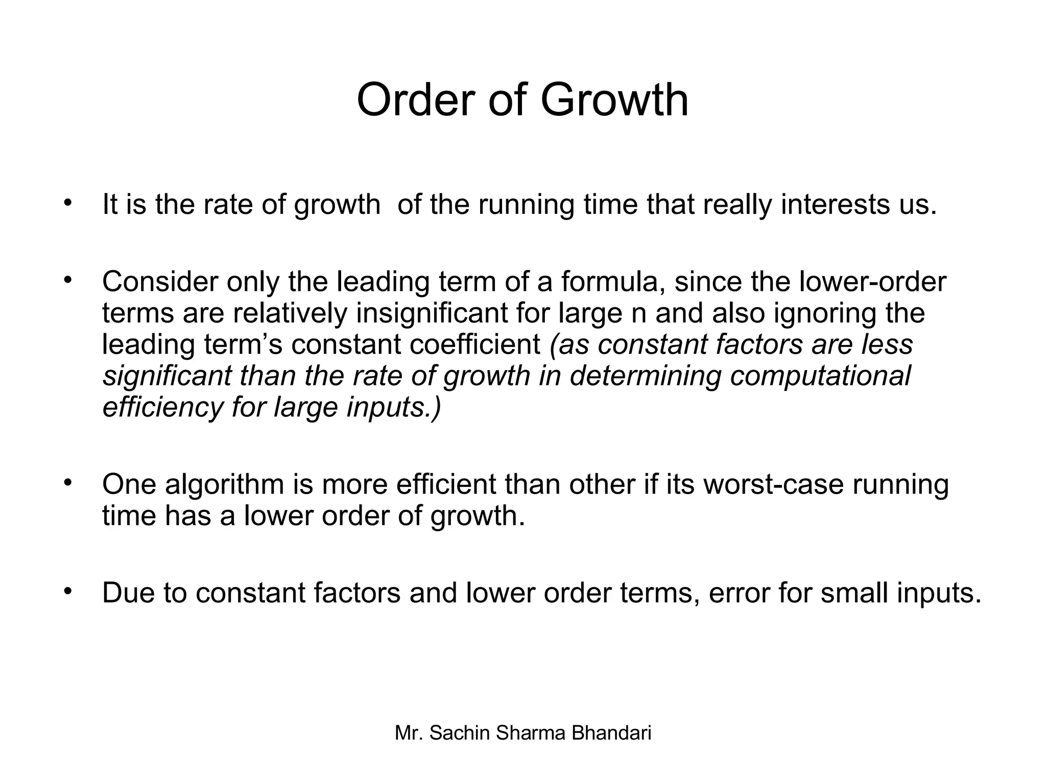
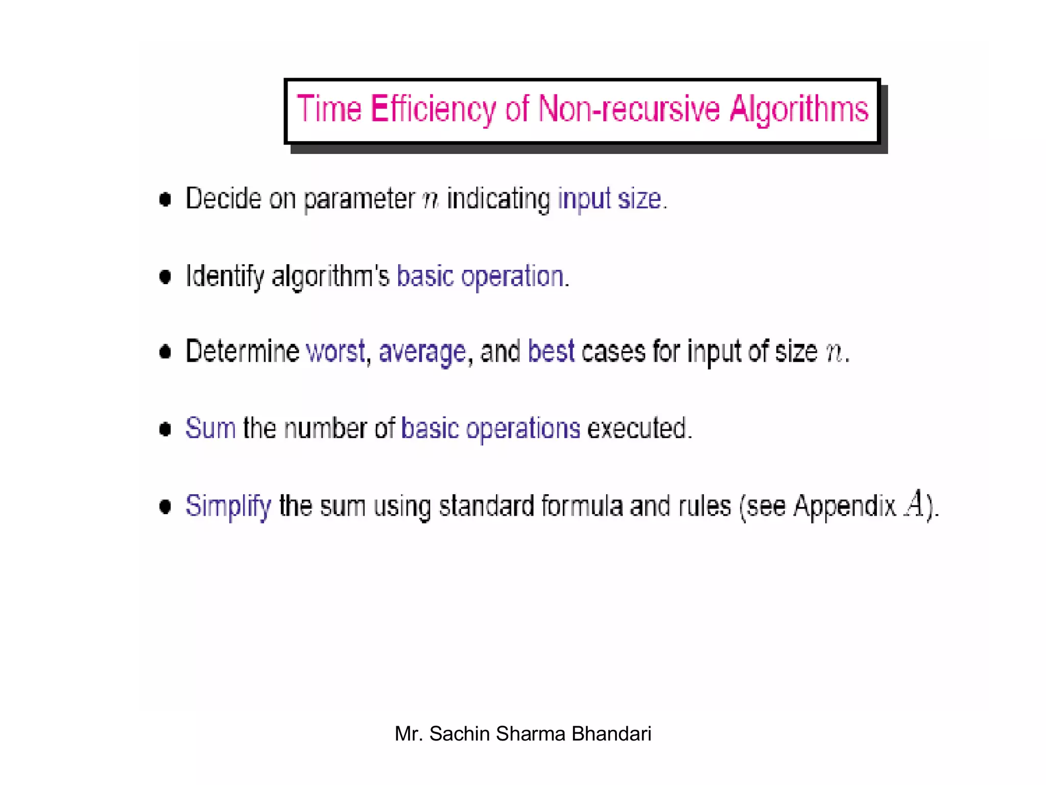
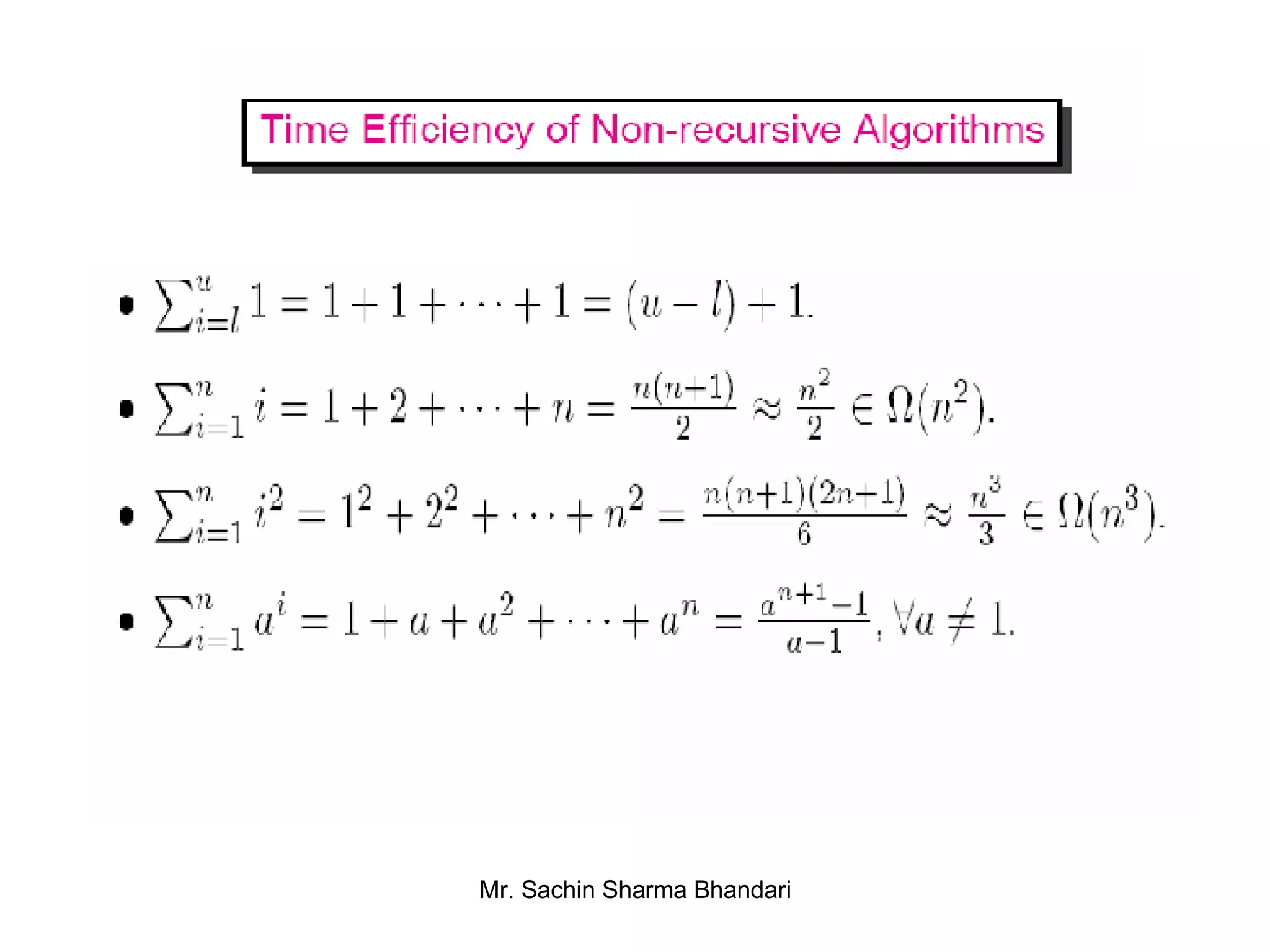
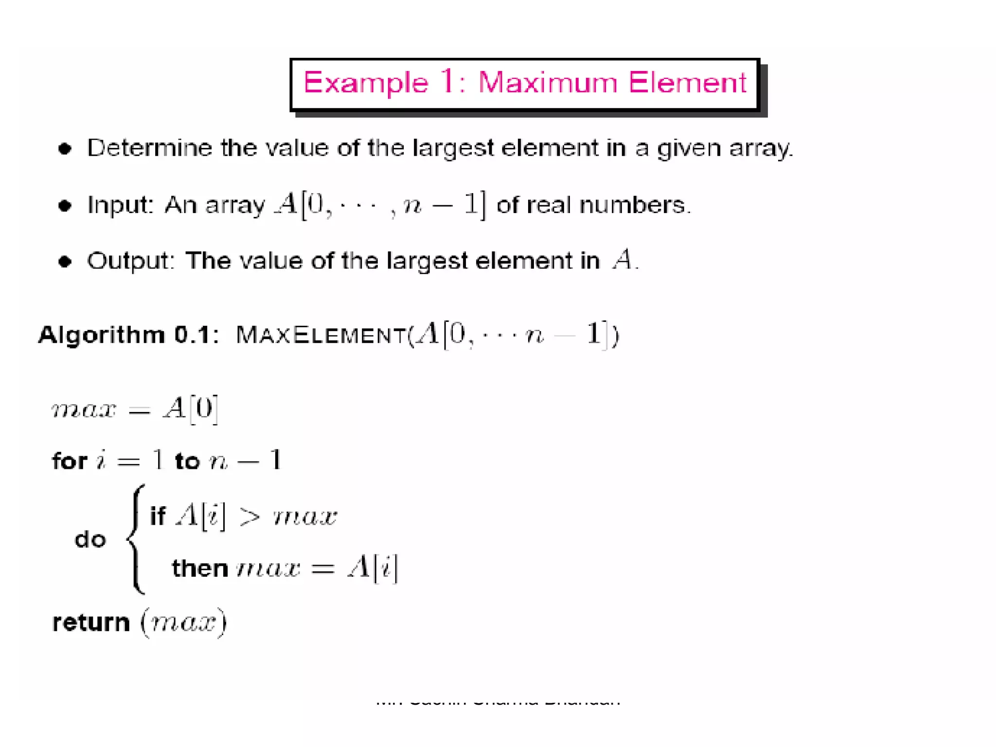
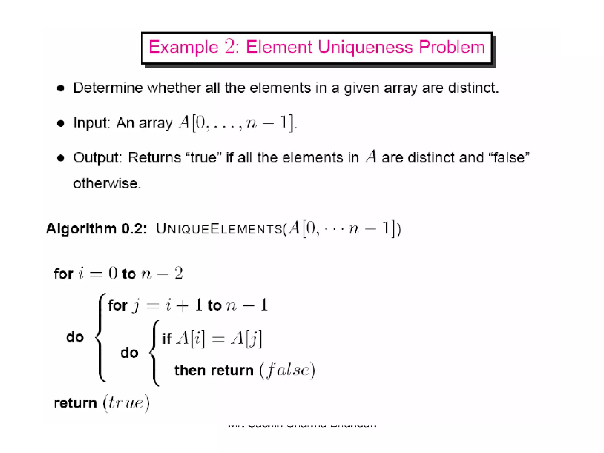
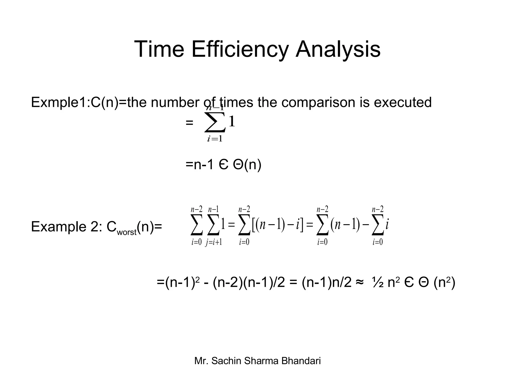
- Measuring an algorithm's time efficiency based on input size and number of basic operations.
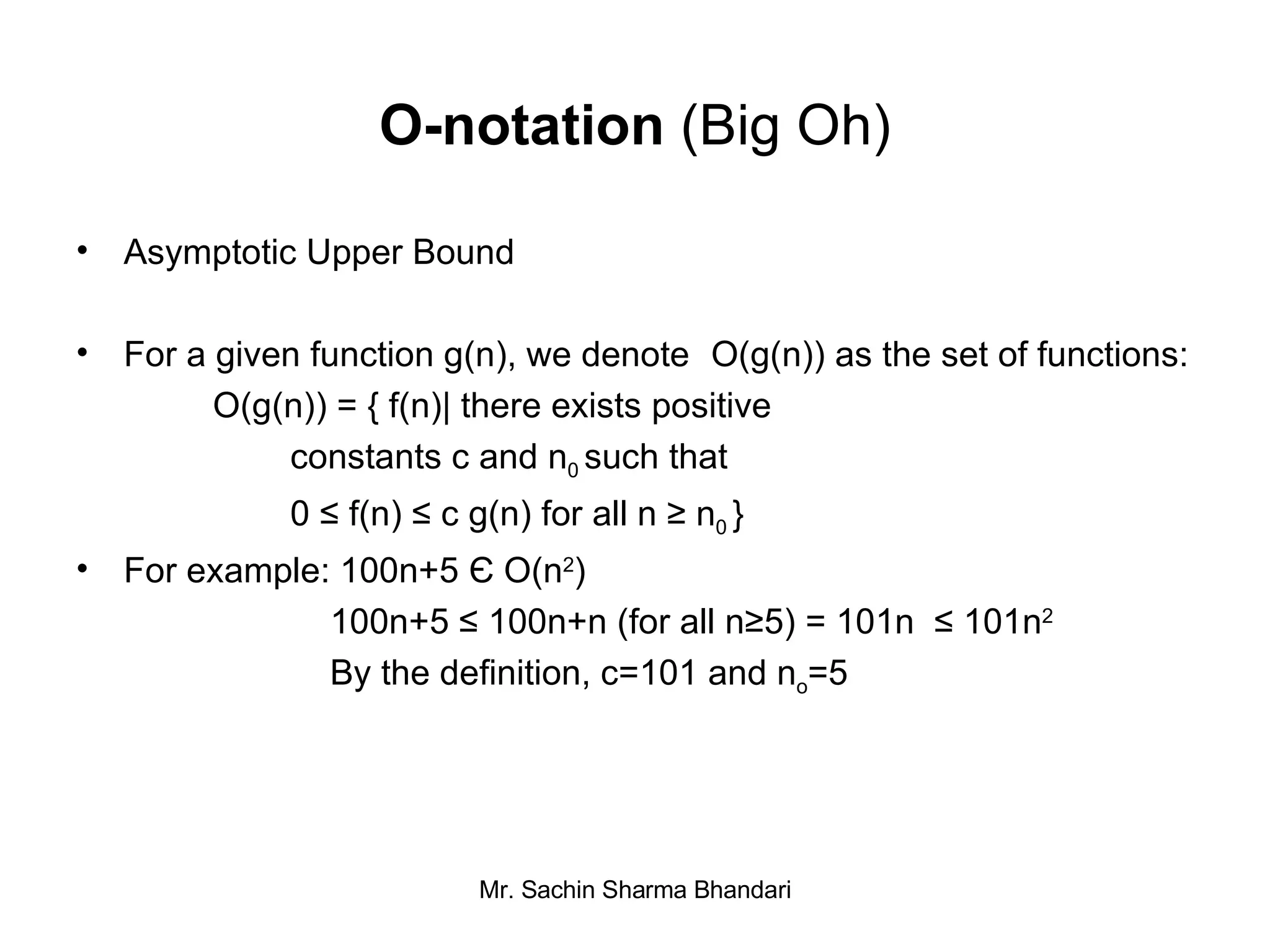
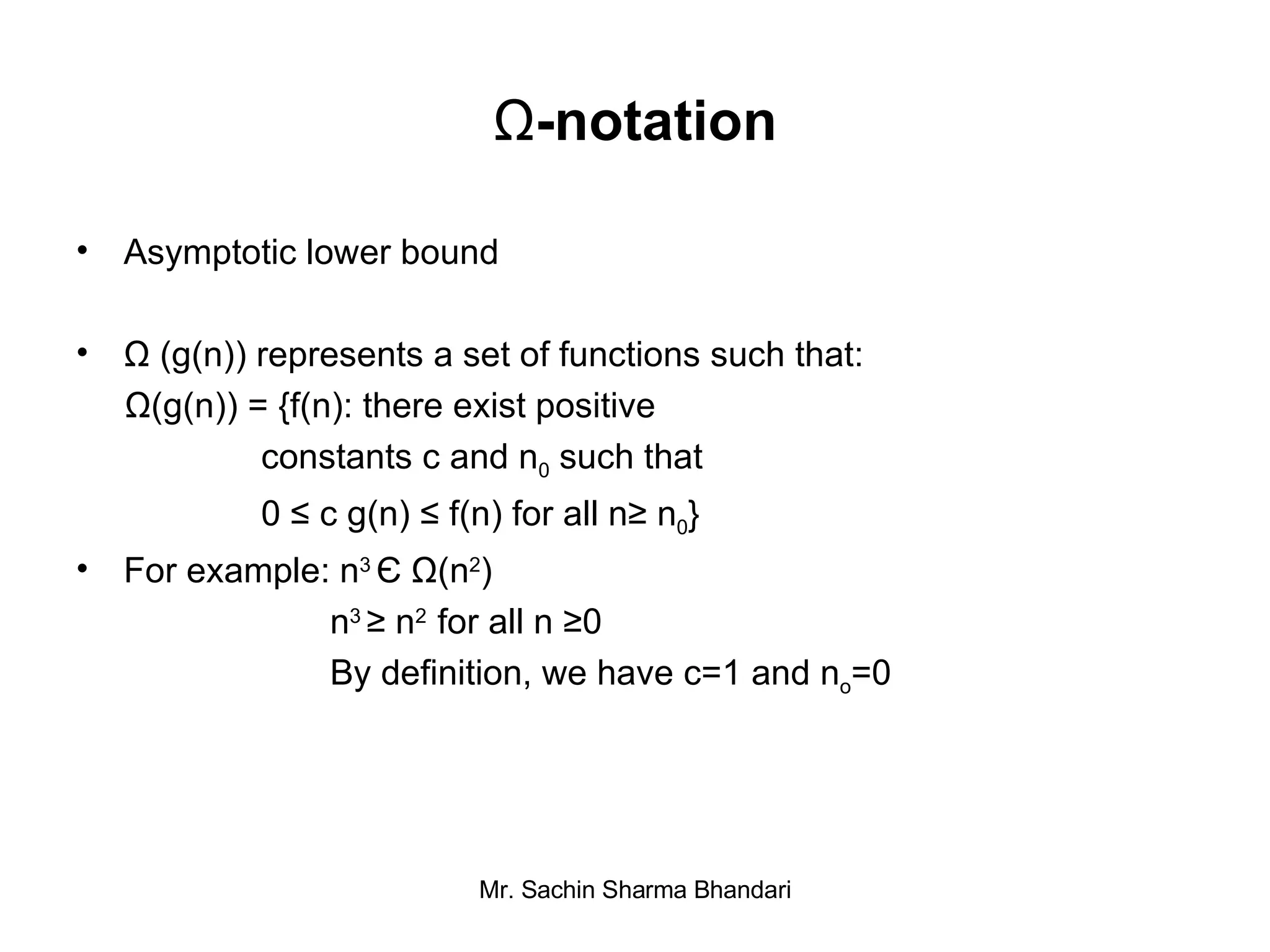
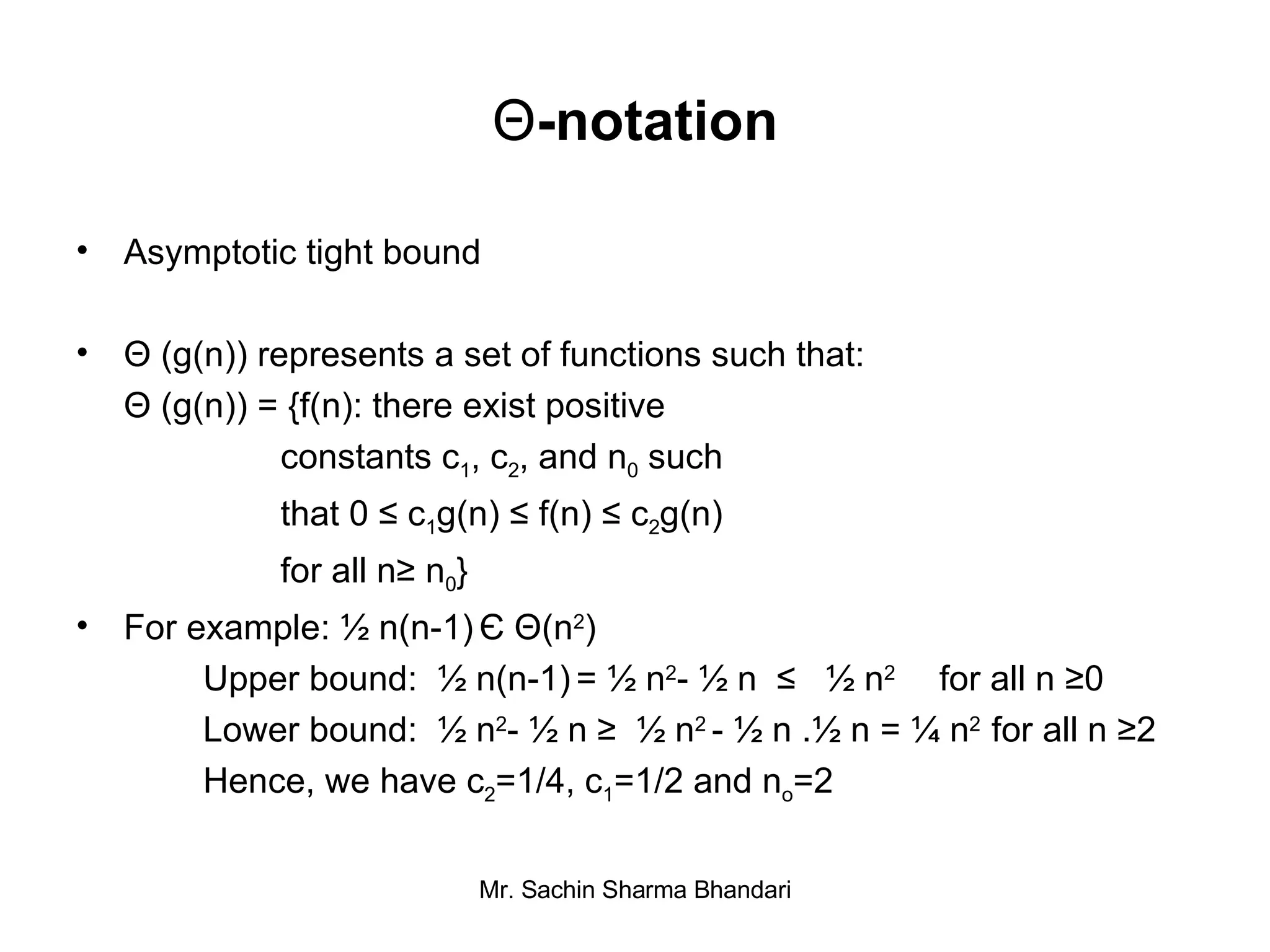
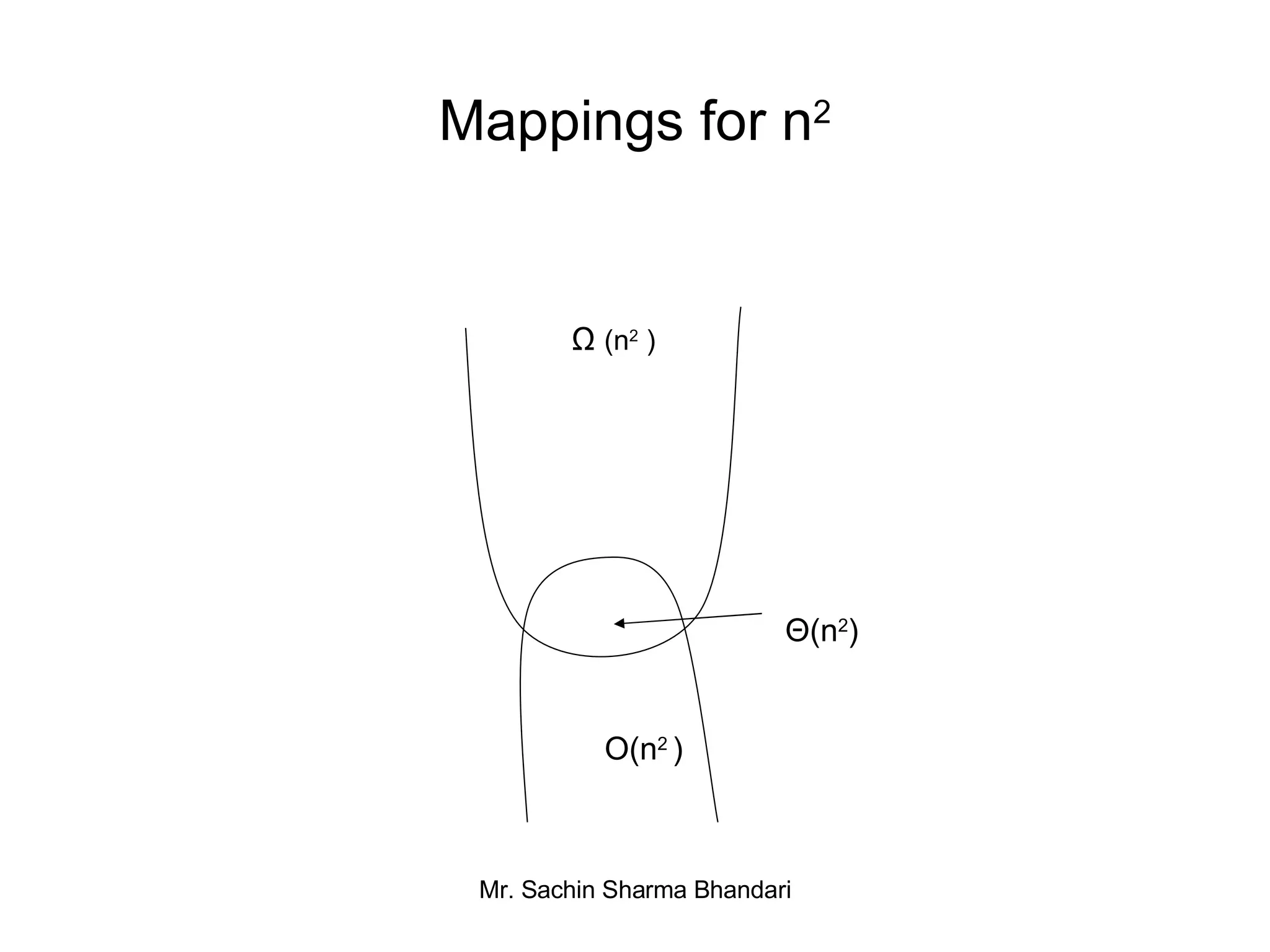
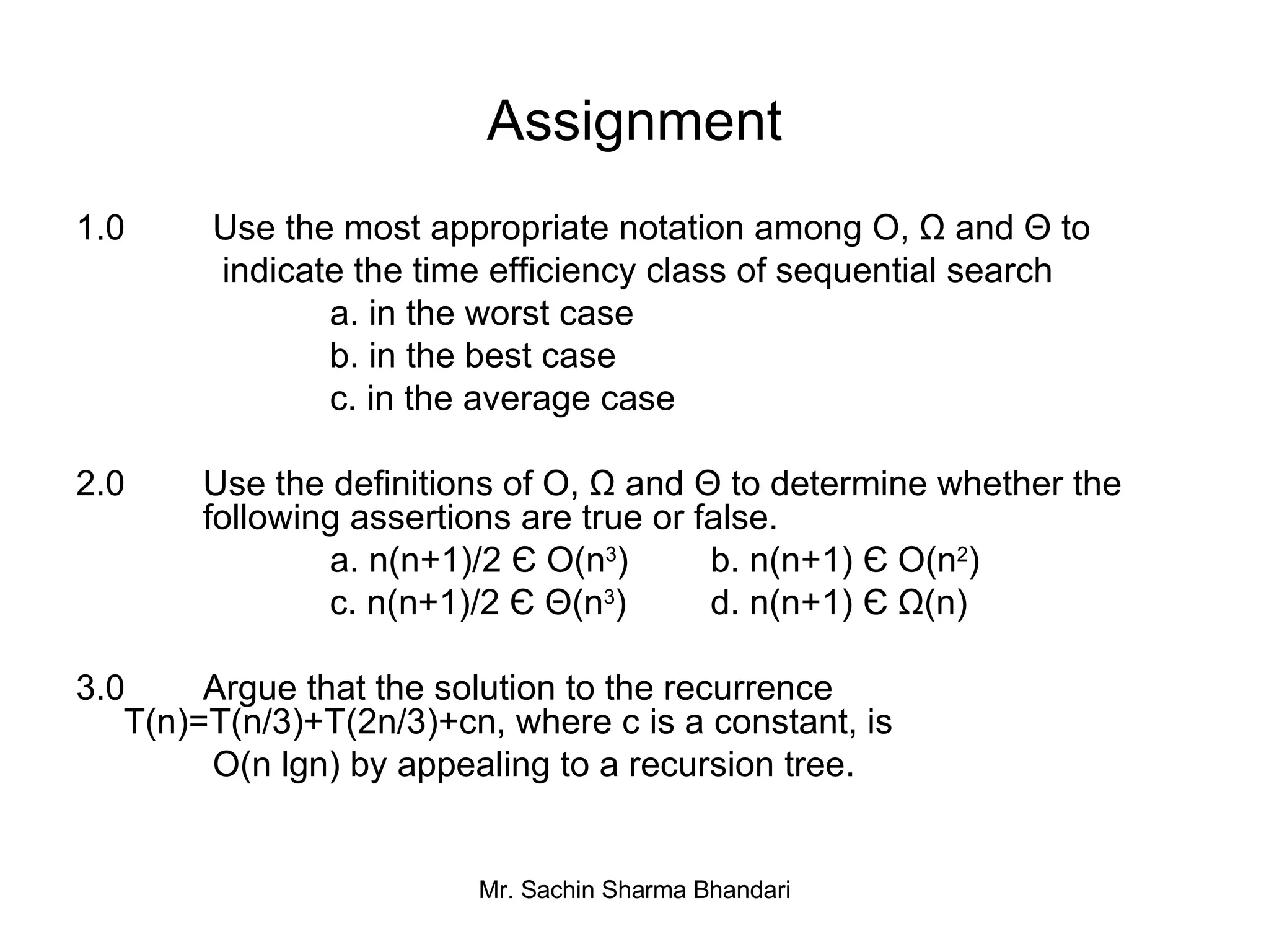
- Using asymptotic notations like O, Ω, Θ to classify algorithms by order of growth.
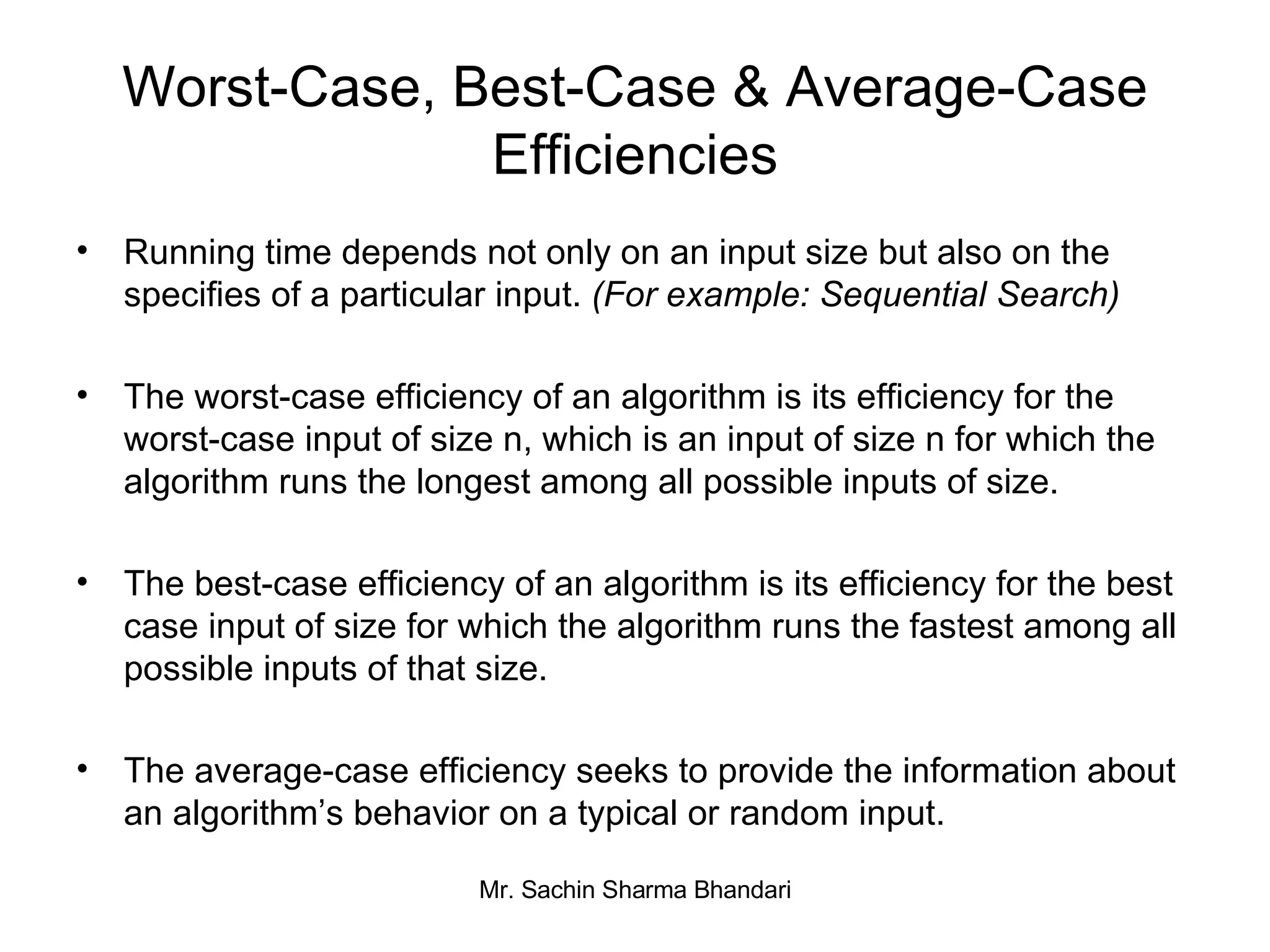
- Analyzing worst-case, best-case, and average-case efficiencies.
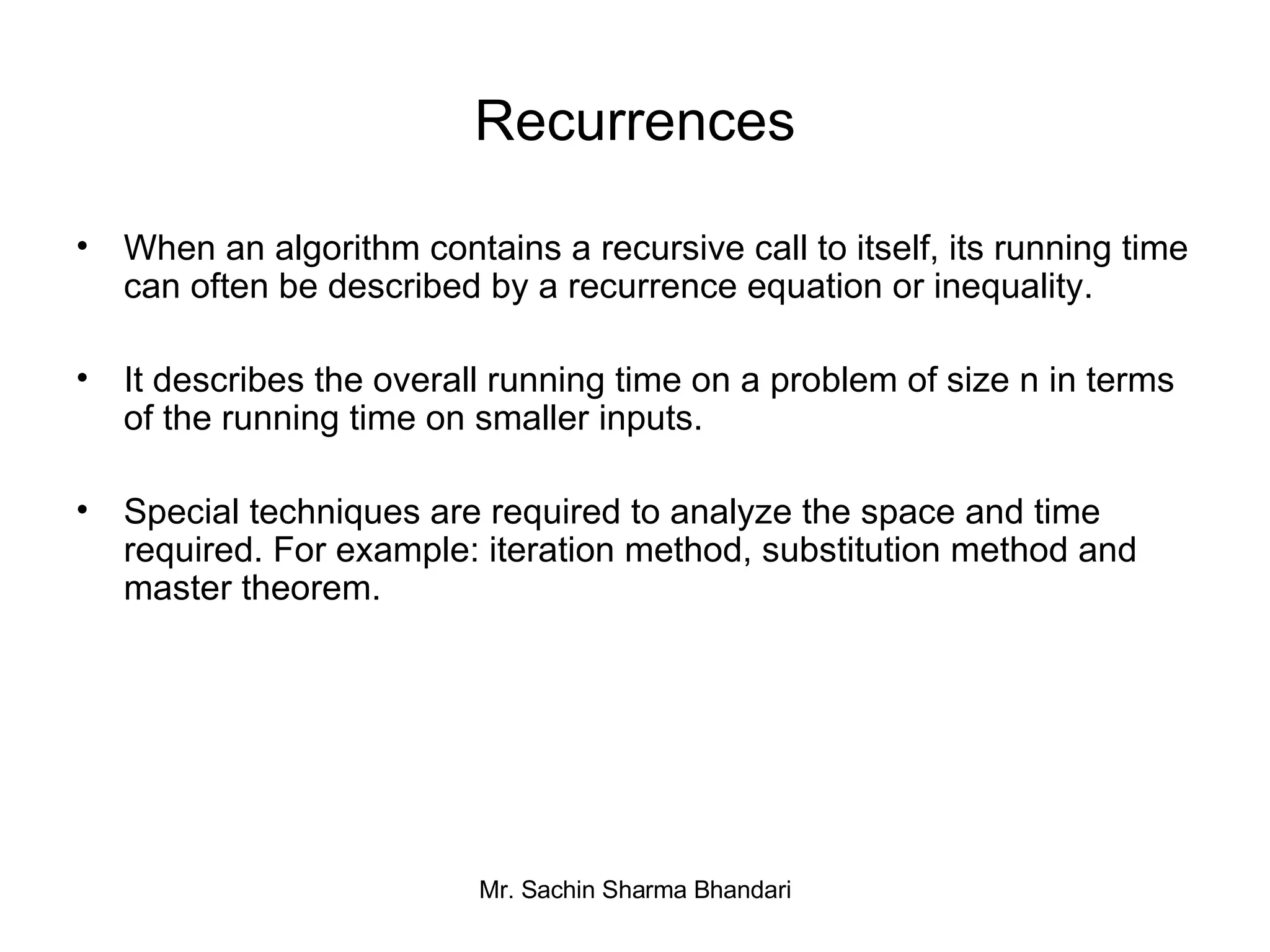
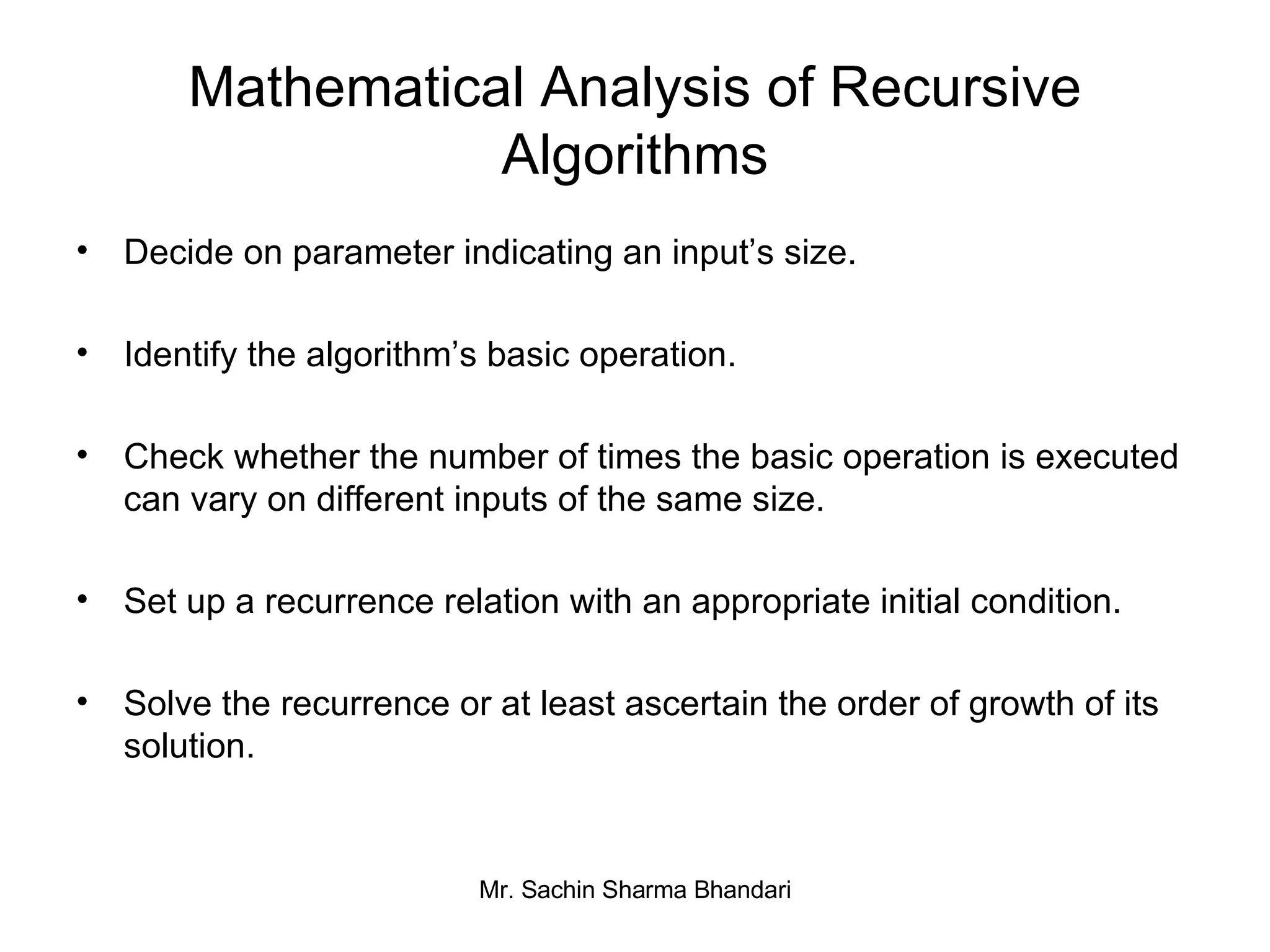
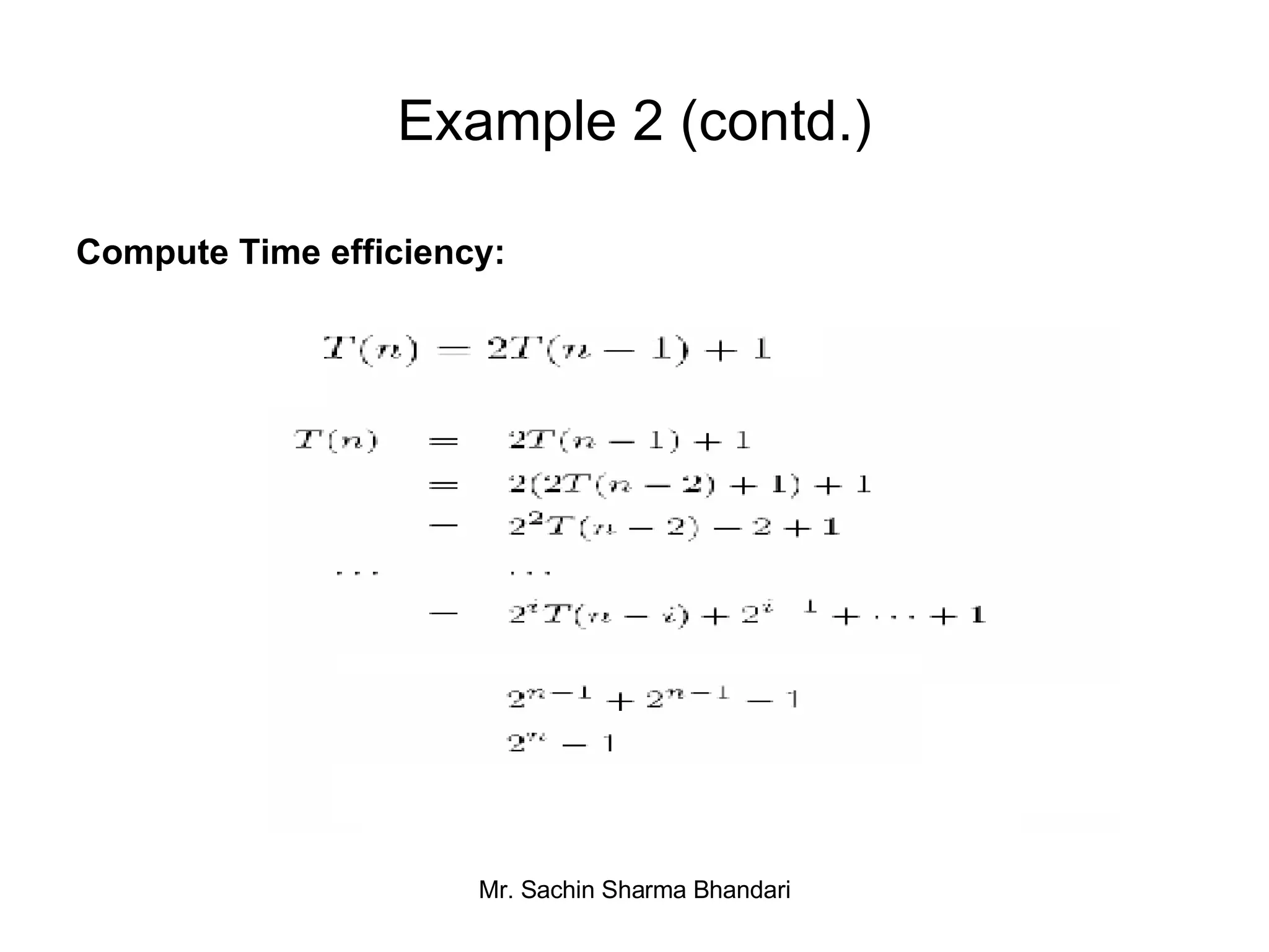
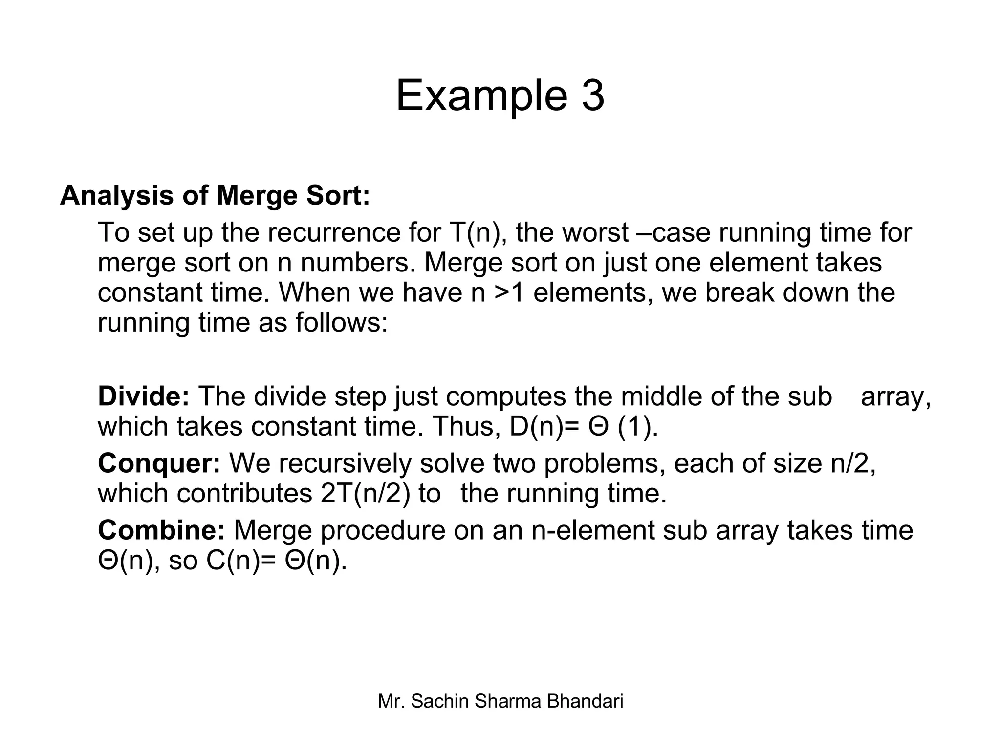
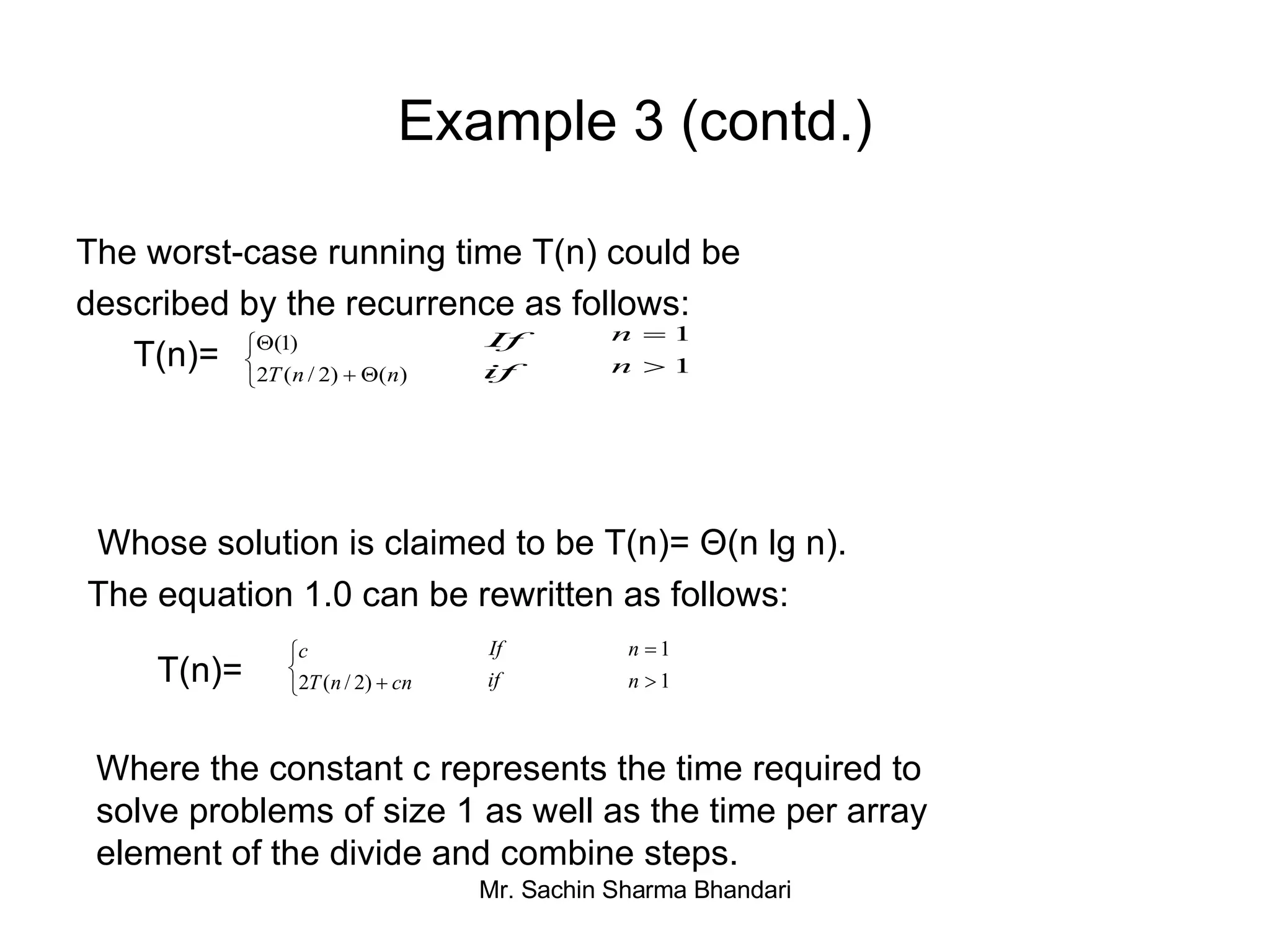
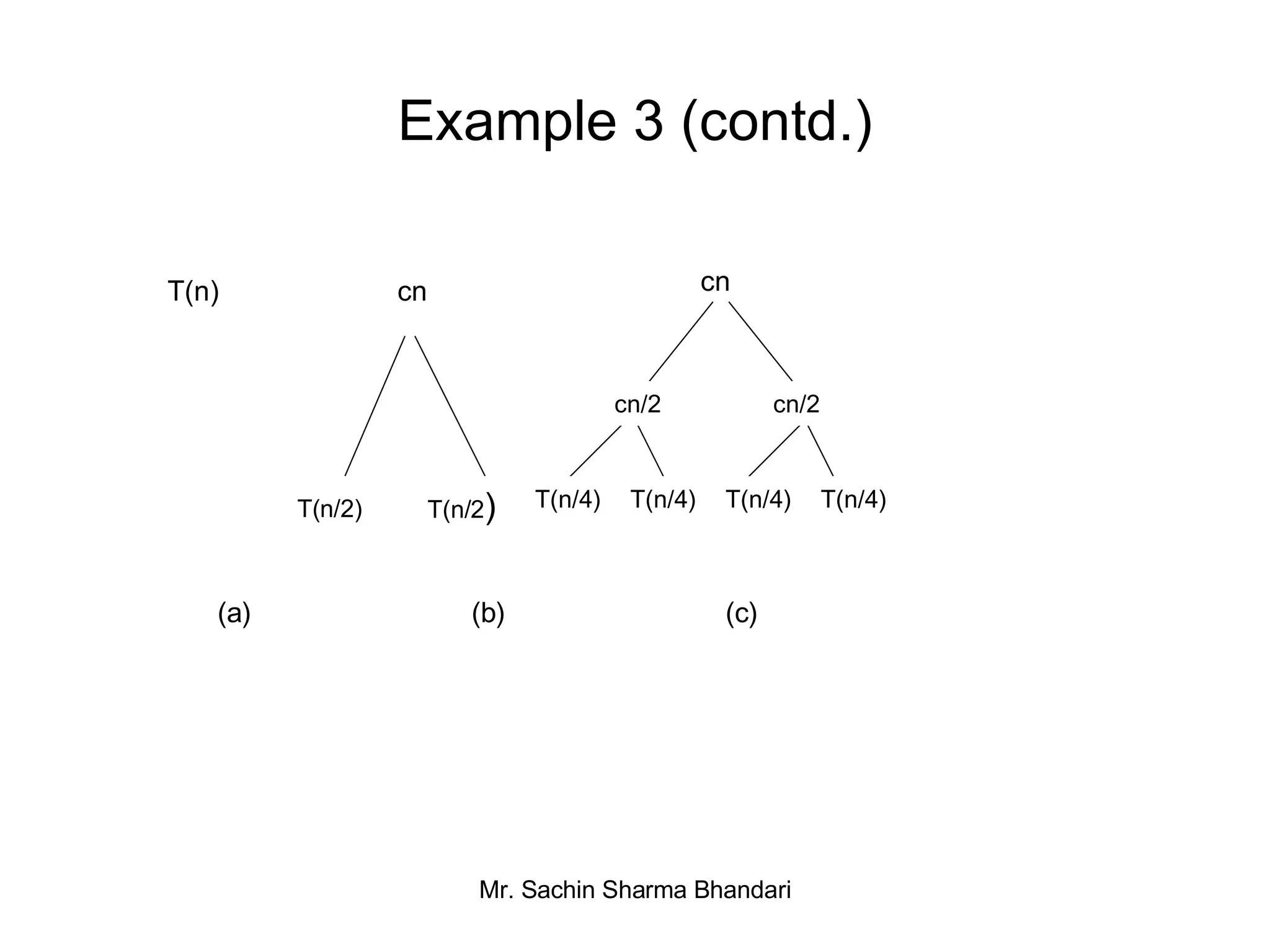
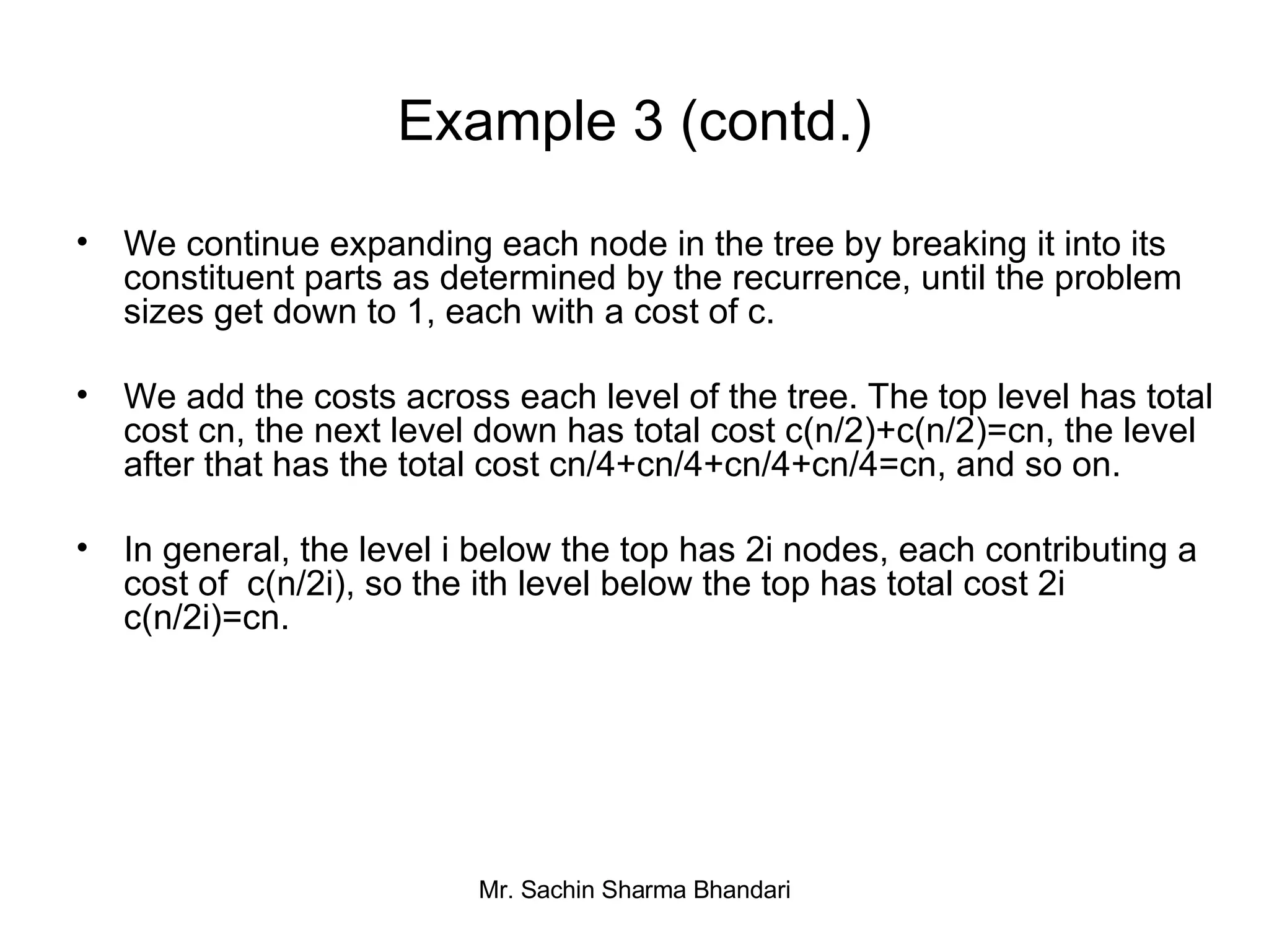
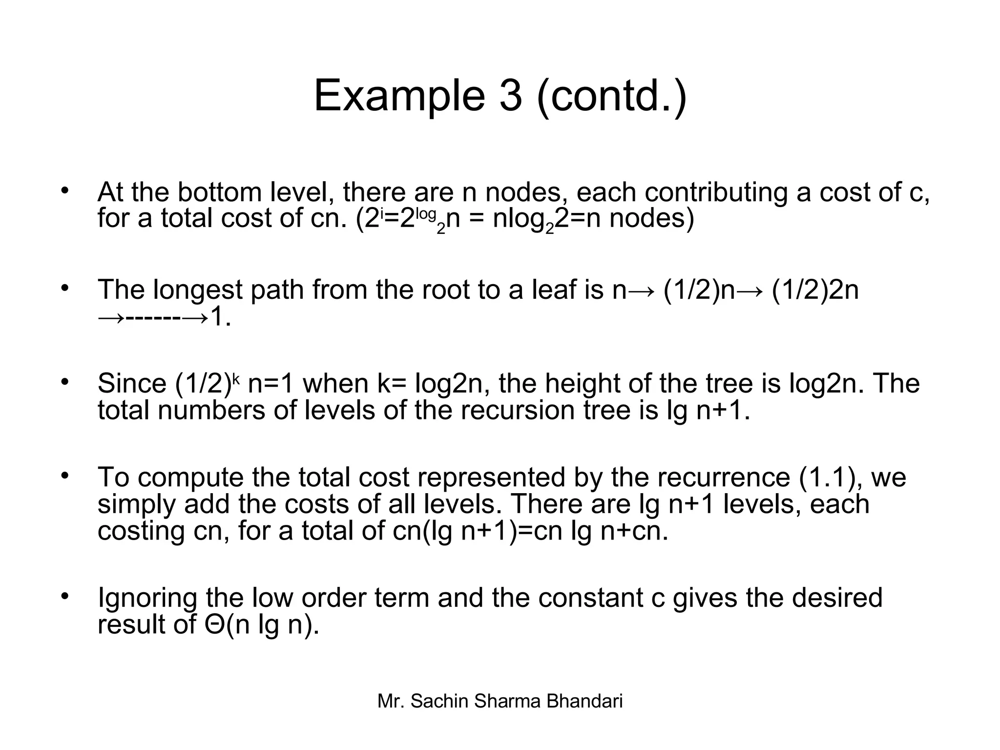
- Setting up recurrence relations to analyze recursive algorithms like merge sort.


![Sequential Search Algorithm: Sequential search (A[0..n-1],k) // searches for a given value in a given array by sequential search // Input: An array A[0..n-1] and a search key k // Output: The index of the first element of A that matches k or -1 if there are no matching elements. i=0 While i<n and A [i] ≠k do i=i+1 If i<n return i Else return -1](https://image.slidesharecdn.com/slide2-1194148724361620-2/75/Slide2-5-2048.jpg)
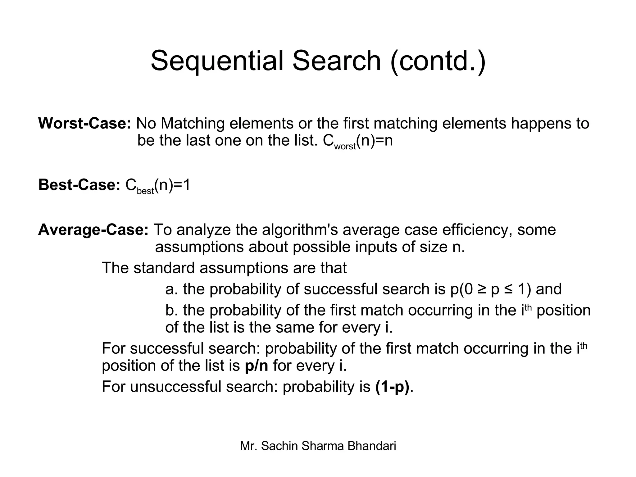
![Sequential Search (contd.) C avg (n)=[1.p/n+2.p/n+..........+i.p/n+.........+n.p/n]+n.(1-p) = p/n[1+2+…….+i+…………+n]+n(1-p) =p/n (n(n+1))/2+n(1-p) =p(n+1)/2+n(1-p) If p=1 (successful search), the average number of key comparisons made by sequential search is (n+1)/2 i.e. the algorithm will inspect half of the list’s elements. If p=0 (unsuccessful search), the average number of key comparisons made by sequential search will be n .](https://image.slidesharecdn.com/slide2-1194148724361620-2/75/Slide2-7-2048.jpg)


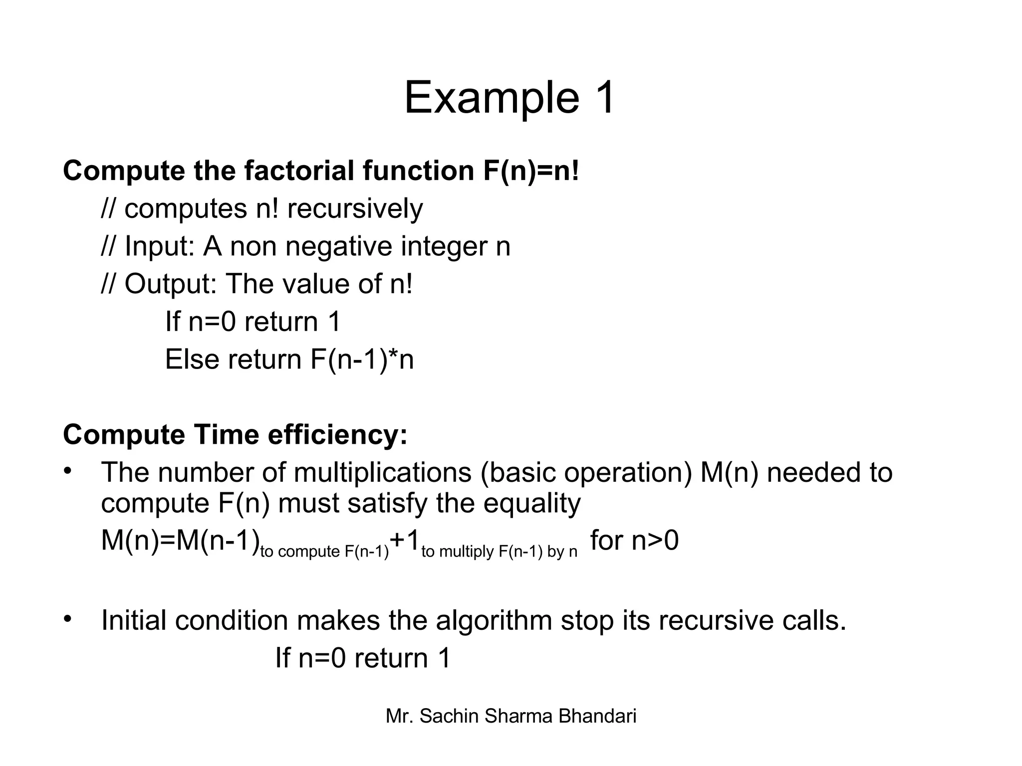
![Example 1 (contd.) From the method of backward substitutions, we have M(n) =M(n-1)+1 substitute M(n-1)=M(n-2)+1 =[M(n-2)+1]+1=M(n-2)+2 substituteM(n-2)=M(n-3)+1 =[M(n-3)+1]+1=M(n-3)+3 . . =M(n-i)+i =………=M(n-n)+n =M(0)+n but M(0)=0 =n](https://image.slidesharecdn.com/slide2-1194148724361620-2/75/Slide2-23-2048.jpg)


![Sequential Search Algorithm: Sequential search (A[0..n-1],k) // searches for a given value in a given array by sequential search // Input: An array A[0..n-1] and a search key k // Output: The index of the first element of A that matches k or -1 if there are no matching elements. i=0 While i<n and A [i] ≠k do i=i+1 If i<n return i Else return -1](https://crownmelresort.com/image.slidesharecdn.com/slide2-1194148724361620-2/75/Slide2-5-2048.jpg)

![Sequential Search (contd.) C avg (n)=[1.p/n+2.p/n+..........+i.p/n+.........+n.p/n]+n.(1-p) = p/n[1+2+…….+i+…………+n]+n(1-p) =p/n (n(n+1))/2+n(1-p) =p(n+1)/2+n(1-p) If p=1 (successful search), the average number of key comparisons made by sequential search is (n+1)/2 i.e. the algorithm will inspect half of the list’s elements. If p=0 (unsuccessful search), the average number of key comparisons made by sequential search will be n .](https://crownmelresort.com/image.slidesharecdn.com/slide2-1194148724361620-2/75/Slide2-7-2048.jpg)


![Example 1 (contd.) From the method of backward substitutions, we have M(n) =M(n-1)+1 substitute M(n-1)=M(n-2)+1 =[M(n-2)+1]+1=M(n-2)+2 substituteM(n-2)=M(n-3)+1 =[M(n-3)+1]+1=M(n-3)+3 . . =M(n-i)+i =………=M(n-n)+n =M(0)+n but M(0)=0 =n](https://crownmelresort.com/image.slidesharecdn.com/slide2-1194148724361620-2/75/Slide2-23-2048.jpg)


![Support, Monitoring, Continuous Improvement & Scaling Agentic Automation [3/3]](https://cdn.slidesharecdn.com/ss_thumbnails/agenticcommunityseries-day3-cfd-251120170304-ddef8112-thumbnail.jpg?width=640&height=640&fit=bounds)


