The document covers the concept of recursion as a problem-solving technique, explaining how it divides problems into smaller subproblems, with examples such as the factorial function and Fibonacci numbers. Additionally, it discusses the advantages and disadvantages of recursive algorithms, the divide-and-conquer method, and approaches to solve recurrences through methods like the substitution and iteration methods. It also introduces the Master Theorem for analyzing the running time of divide-and-conquer algorithms.
![Counting Digits
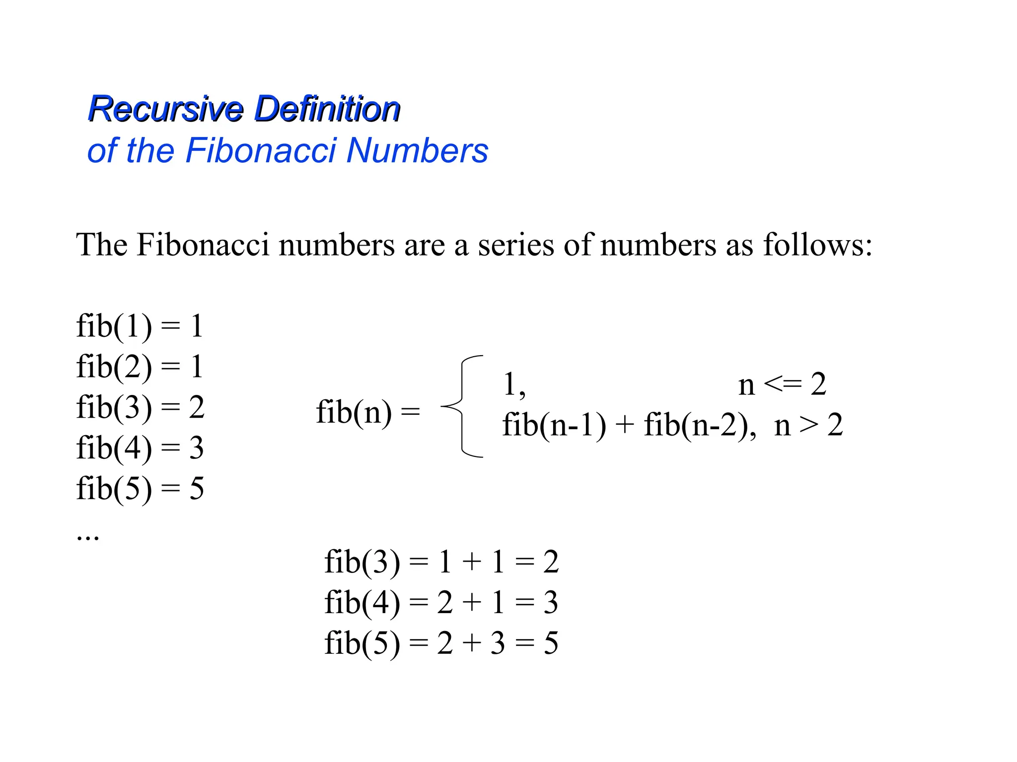
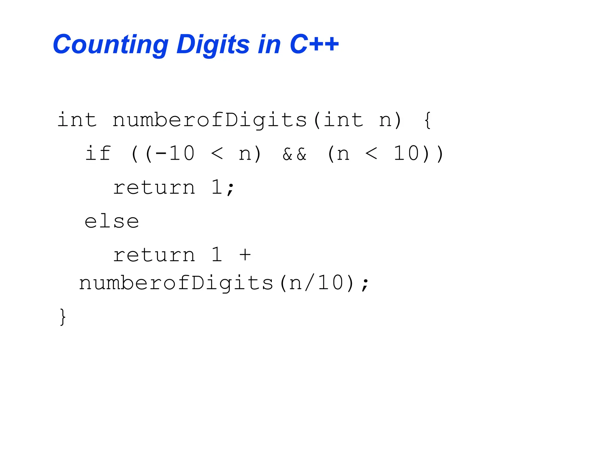
• Recursive definition
digits(n) = 1 if (–9 <= n <= 9)
1 + digits(n/10) otherwise
• Example
digits(321) =
1 + digits(321/10) = 1 +digits(32) =
1 + [1 + digits(32/10)] = 1 + [1 + digits(3)] =
1 + [1 + (1)] =
3](https://image.slidesharecdn.com/3-240917091329-ed94d333/75/3-Recursion-and-Recurrences-ppt-detail-about-recursive-learning-8-2048.jpg)
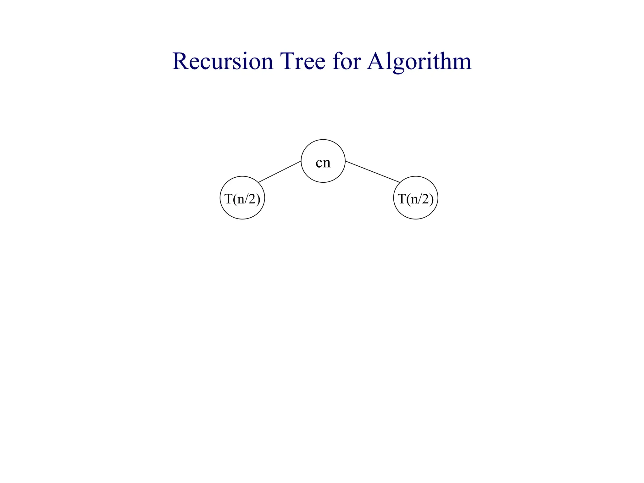
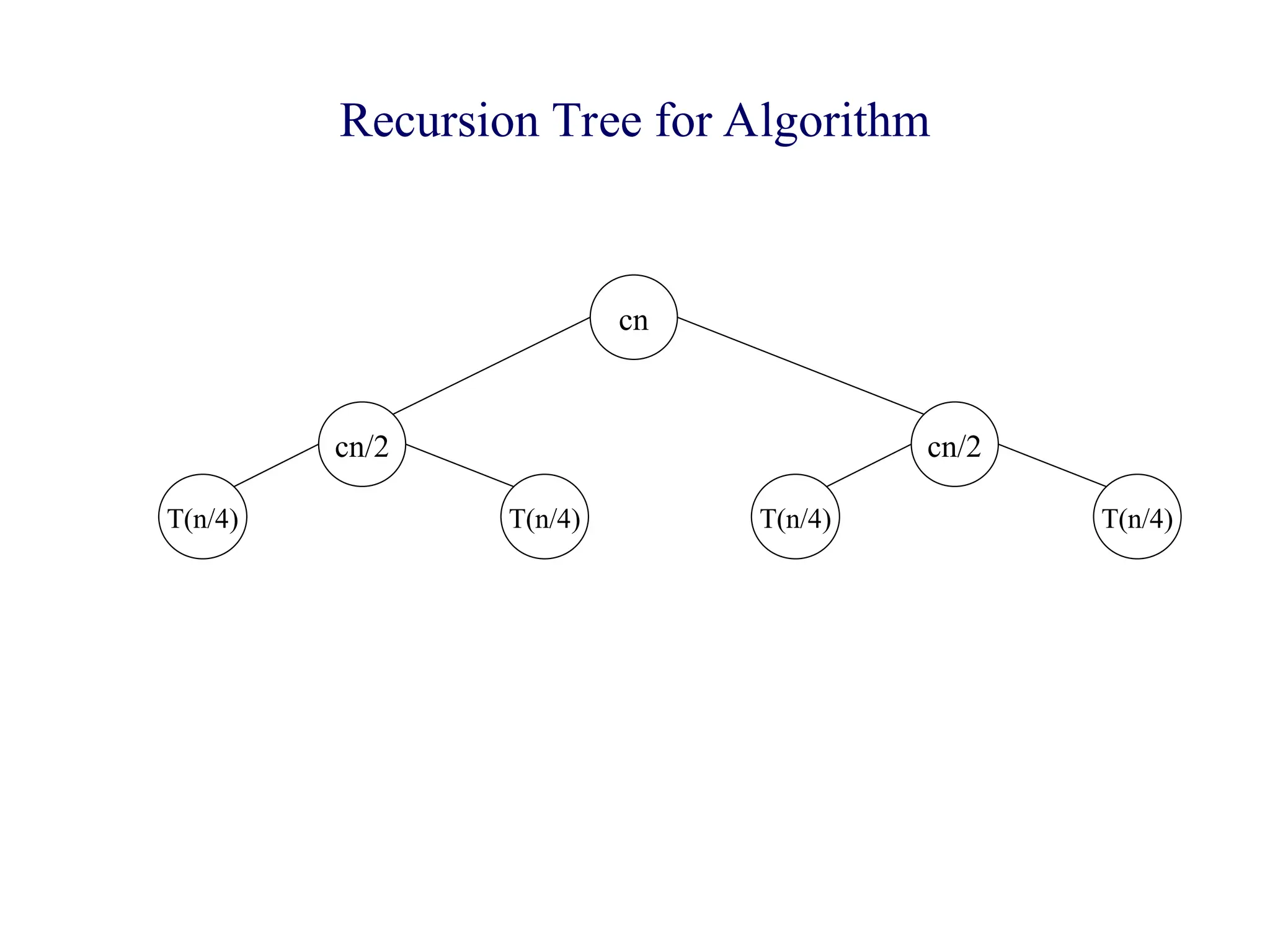
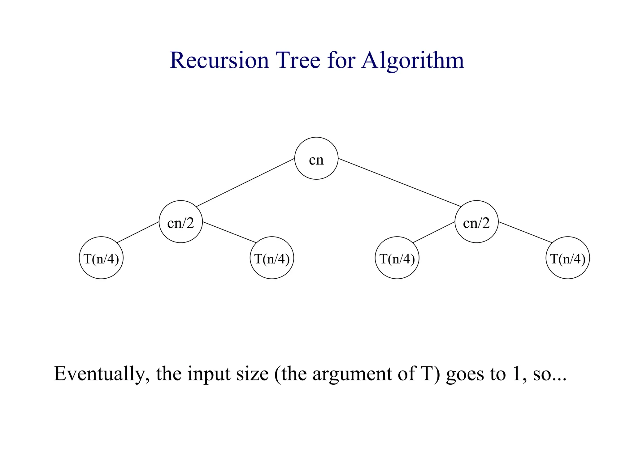
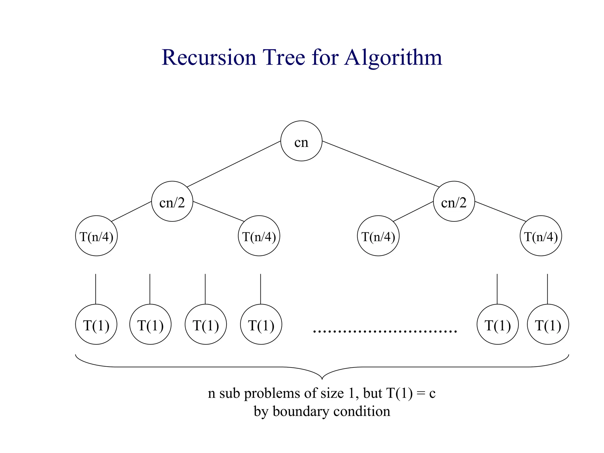
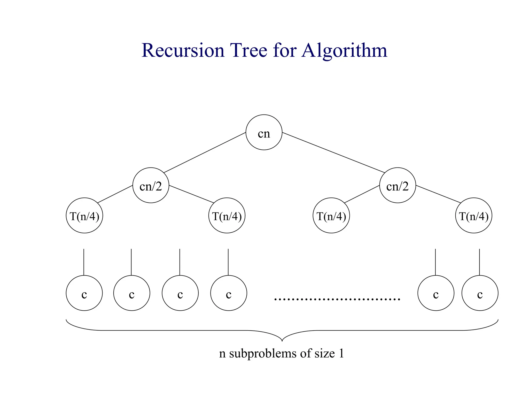
![Recursion Tree for Algorithm
level nodes/ cost/
level level
0 20
= 1 cn
1 21
= 2 cn
2 22
= 4 cn
. .
. .
. .
N-1 2N-1
=n cn
Since 2N-1
= n,
N-1 = lg(n)
levels = N = 1+lg(n)
T(n) = total cost = (levels)(cost/level)
T(n) = cn [1+lg(n)] = O( n lg(n))
n nodes at level N-1](https://image.slidesharecdn.com/3-240917091329-ed94d333/75/3-Recursion-and-Recurrences-ppt-detail-about-recursive-learning-39-2048.jpg)


![Counting Digits
• Recursive definition
digits(n) = 1 if (–9 <= n <= 9)
1 + digits(n/10) otherwise
• Example
digits(321) =
1 + digits(321/10) = 1 +digits(32) =
1 + [1 + digits(32/10)] = 1 + [1 + digits(3)] =
1 + [1 + (1)] =
3](https://crownmelresort.com/image.slidesharecdn.com/3-240917091329-ed94d333/75/3-Recursion-and-Recurrences-ppt-detail-about-recursive-learning-8-2048.jpg)


![Recursion Tree for Algorithm
level nodes/ cost/
level level
0 20
= 1 cn
1 21
= 2 cn
2 22
= 4 cn
. .
. .
. .
N-1 2N-1
=n cn
Since 2N-1
= n,
N-1 = lg(n)
levels = N = 1+lg(n)
T(n) = total cost = (levels)(cost/level)
T(n) = cn [1+lg(n)] = O( n lg(n))
n nodes at level N-1](https://crownmelresort.com/image.slidesharecdn.com/3-240917091329-ed94d333/75/3-Recursion-and-Recurrences-ppt-detail-about-recursive-learning-39-2048.jpg)