Downloaded 101 times


![Preconditioned System
𝒙 𝒌+𝟏 = 𝑮 𝝎 𝒙 𝒌 + 𝒇 𝝎
𝐺 𝐺𝑆 𝐴 = 𝐼 − (𝐷 − 𝐸)−1 𝐴𝐺𝐽𝐴 𝐴 = 𝐼 − 𝐷−1 𝐴,
𝒙 𝒌+𝟏 = 𝑴−𝟏
𝑵𝒙 𝒌 + 𝑴−𝟏
𝒃
We have two forms for iterative method
Ex)
𝐺 = 𝑀−1
𝑁 = 𝑀−1
𝑀 − 𝐴 = 𝐼 − 𝑀−1
𝐴 𝑓 = 𝑀−1
𝑏
𝐼 − 𝐺 𝑥 = 𝑓
Another view…
[𝐼 − (𝐼 − 𝑀−1
𝐴)]𝑥 = 𝑓
𝑀−1
𝐴𝑥 = 𝑓
𝑴−𝟏
𝑨𝒙 = 𝑴−𝟏
𝒃 Preconditioner 𝑀](https://image.slidesharecdn.com/141206labmeetinglinearsystemspublic-141216055915-conversion-gate02/75/Solving-Poisson-Equation-using-Conjugate-Gradient-Method-and-its-implementation-8-2048.jpg)


![Preconditioned System
𝒙 𝒌+𝟏 = 𝑮 𝝎 𝒙 𝒌 + 𝒇 𝝎
𝐺 𝐺𝑆 𝐴 = 𝐼 − (𝐷 − 𝐸)−1 𝐴𝐺𝐽𝐴 𝐴 = 𝐼 − 𝐷−1 𝐴,
𝒙 𝒌+𝟏 = 𝑴−𝟏
𝑵𝒙 𝒌 + 𝑴−𝟏
𝒃
We have two forms for iterative method
Ex)
𝐺 = 𝑀−1
𝑁 = 𝑀−1
𝑀 − 𝐴 = 𝐼 − 𝑀−1
𝐴 𝑓 = 𝑀−1
𝑏
𝐼 − 𝐺 𝑥 = 𝑓
Another view…
[𝐼 − (𝐼 − 𝑀−1
𝐴)]𝑥 = 𝑓
𝑀−1
𝐴𝑥 = 𝑓
𝑴−𝟏
𝑨𝒙 = 𝑴−𝟏
𝒃 Preconditioner 𝑀](https://crownmelresort.com/image.slidesharecdn.com/141206labmeetinglinearsystemspublic-141216055915-conversion-gate02/75/Solving-Poisson-Equation-using-Conjugate-Gradient-Method-and-its-implementation-8-2048.jpg)


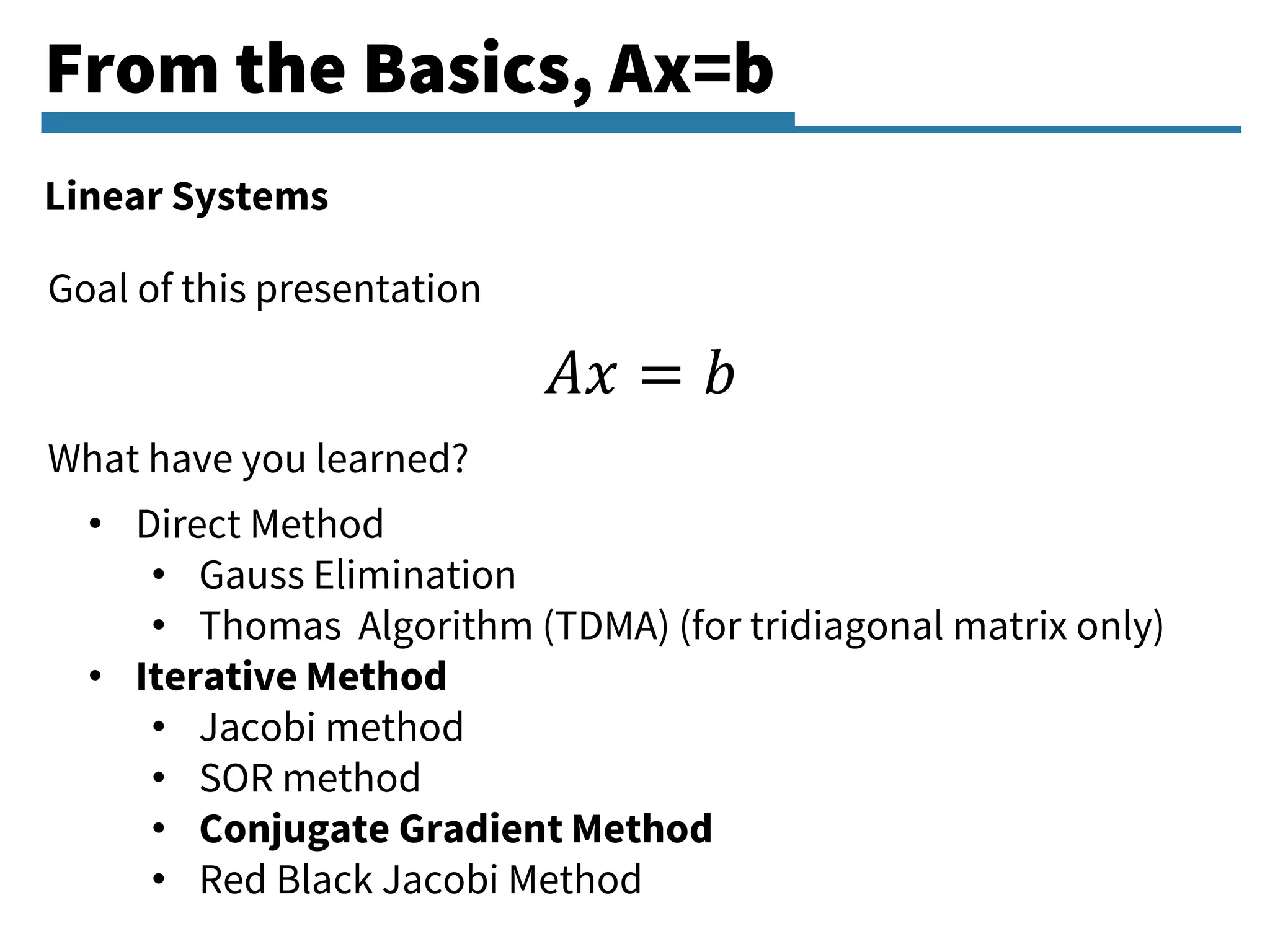
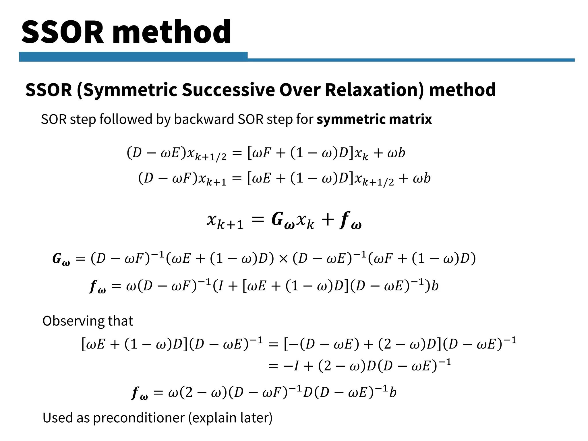
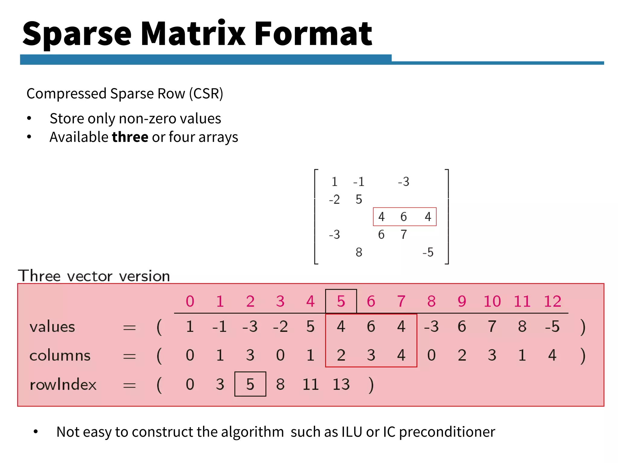
The document presents a thorough exploration of solving the Poisson equation using the conjugate gradient method, detailing various iterative techniques including Jacobi, Gauss-Seidel, and Successive Over-Relaxation (SOR). It discusses the implementation of these methods for large sparse matrices, the use of preconditioners, and the utility of the Intel Math Kernel Library (MKL) for efficient computation. Additionally, the document covers optimization strategies and references key literature on the subject.
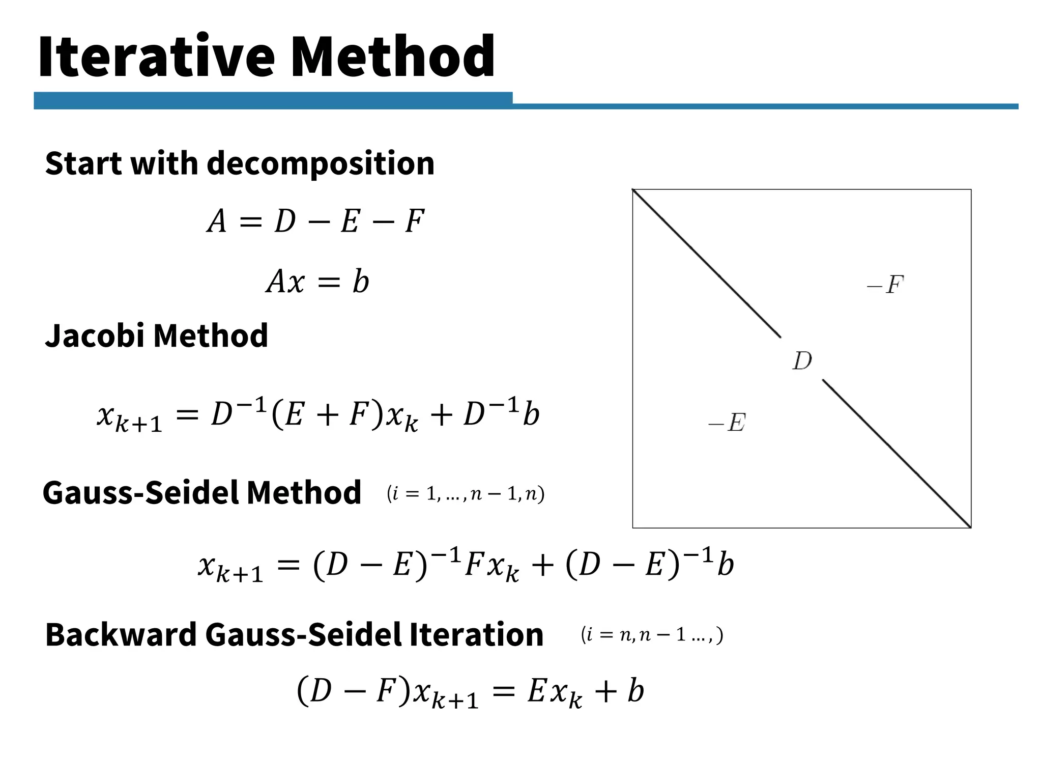
Introduction to the Poisson equation. Discussion on methods like Direct, Jacobi, SOR, and Conjugate Gradient for solving linear systems.
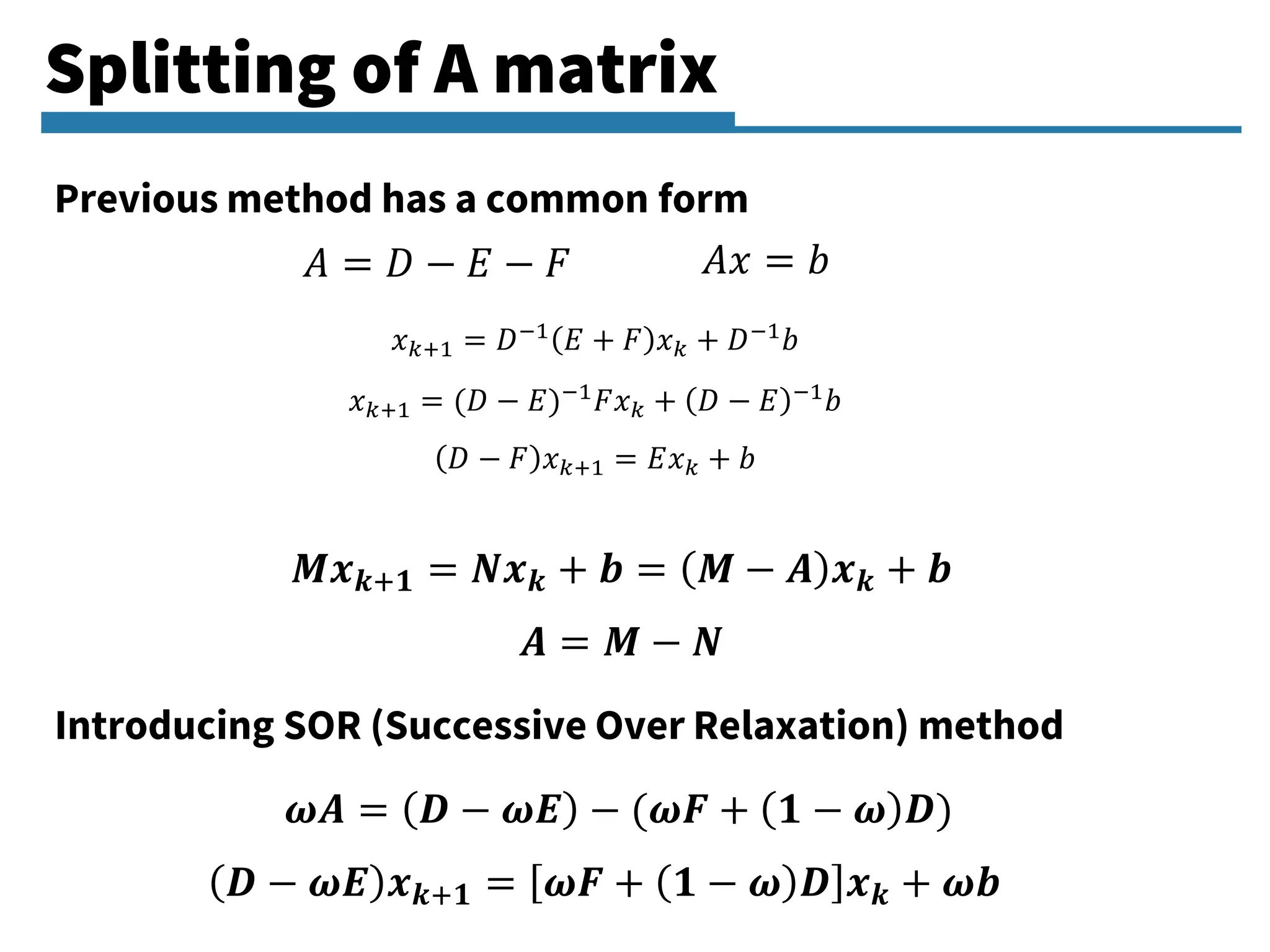
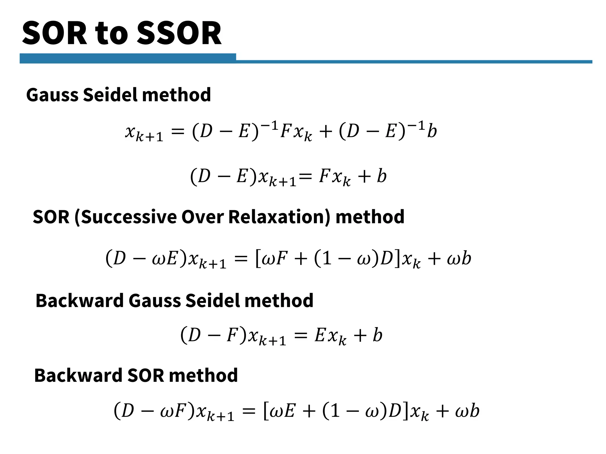
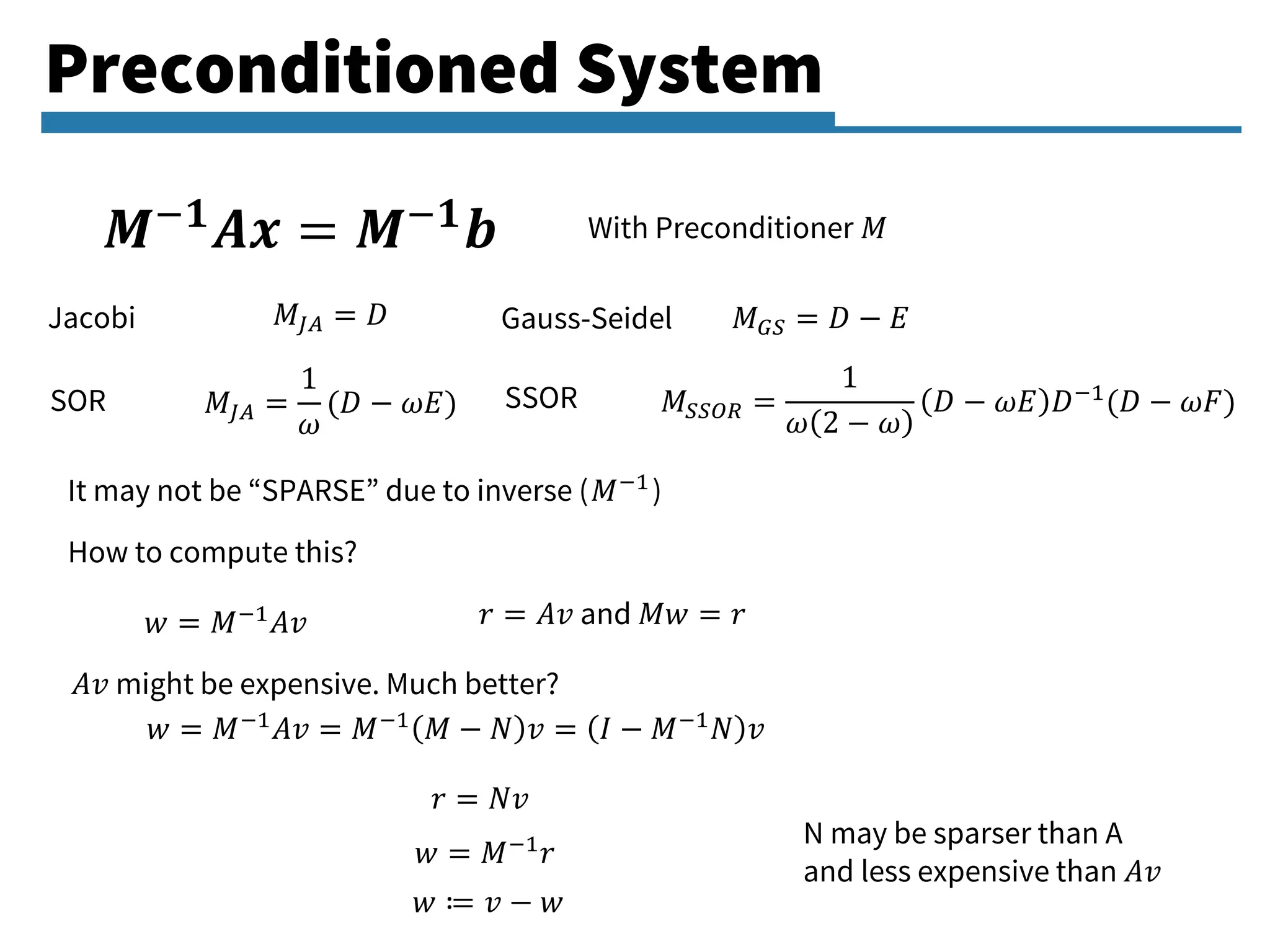
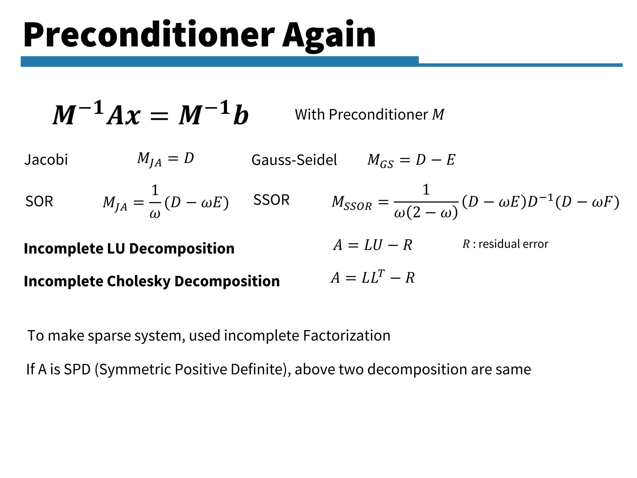
Discussion of SOR, SSOR, and preconditioned iterative methods in solving linear systems, emphasizing matrix decomposition.
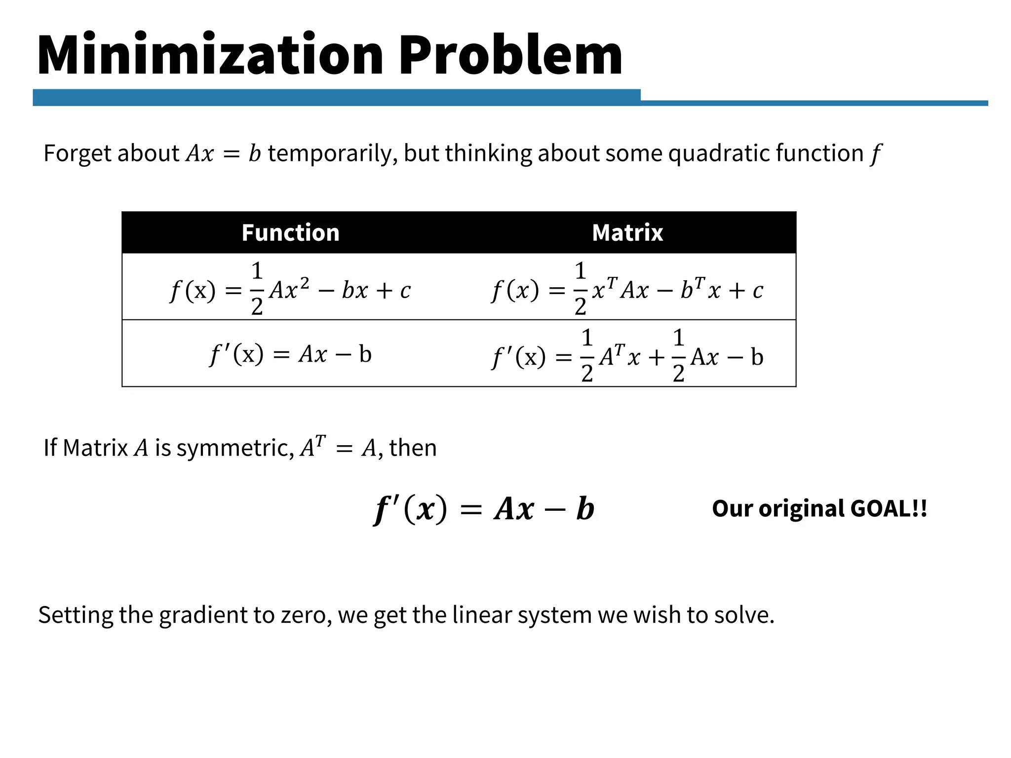
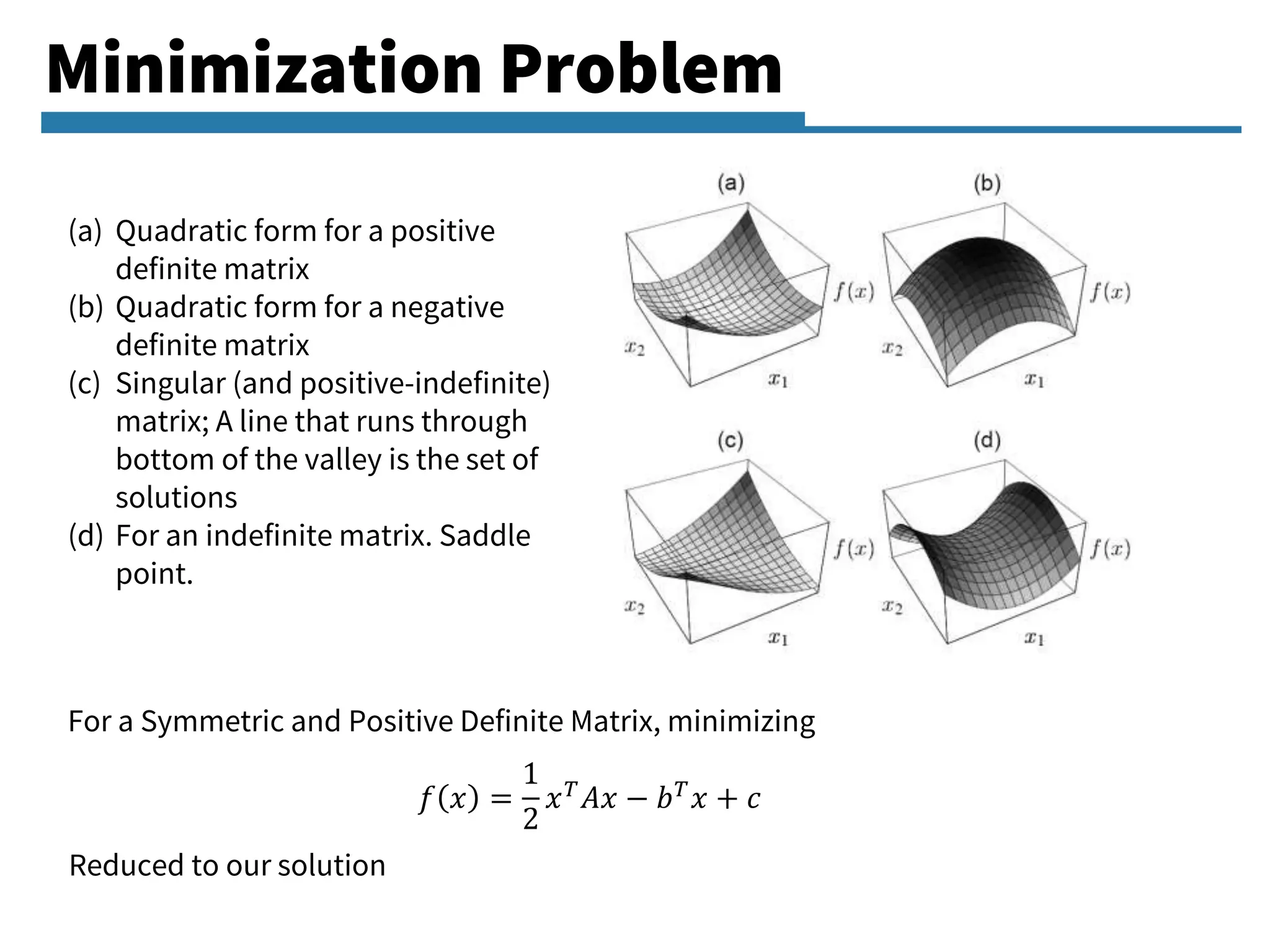
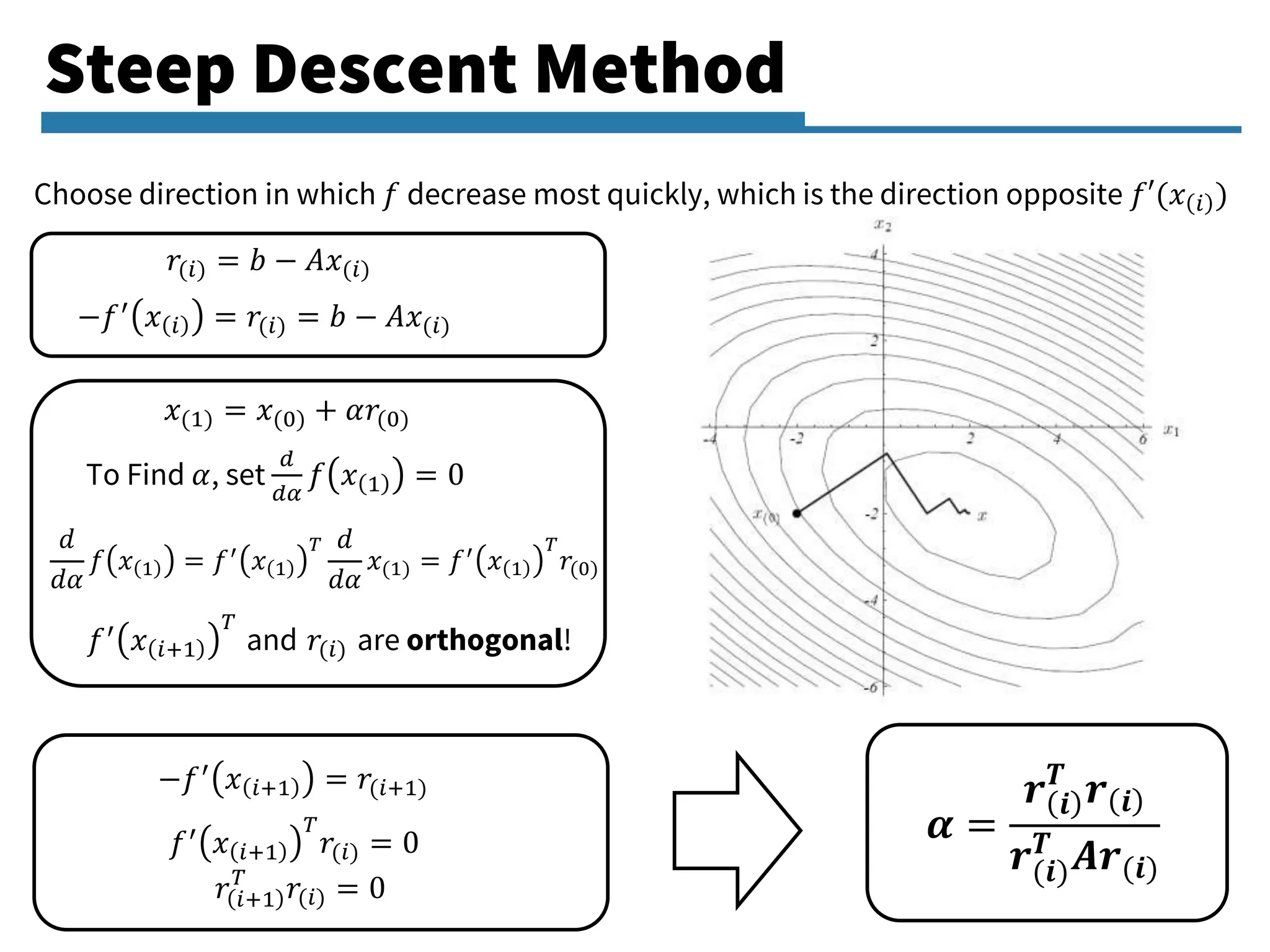
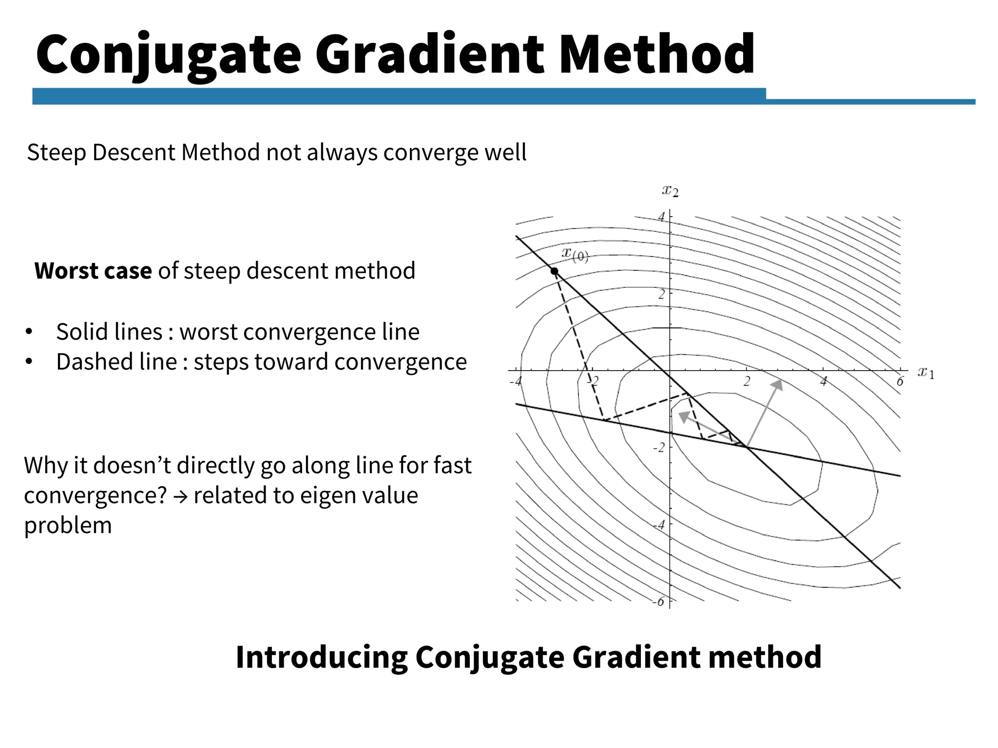
Focusing on the minimization problems related to quadratic functions using gradient methods.
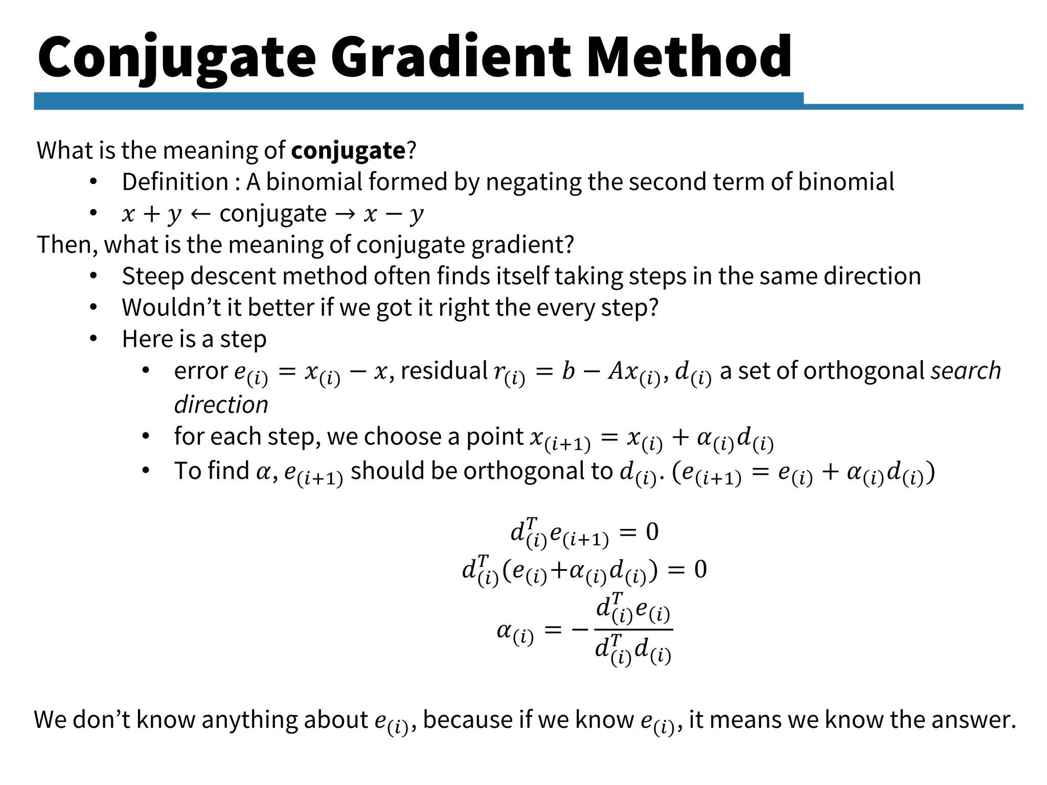
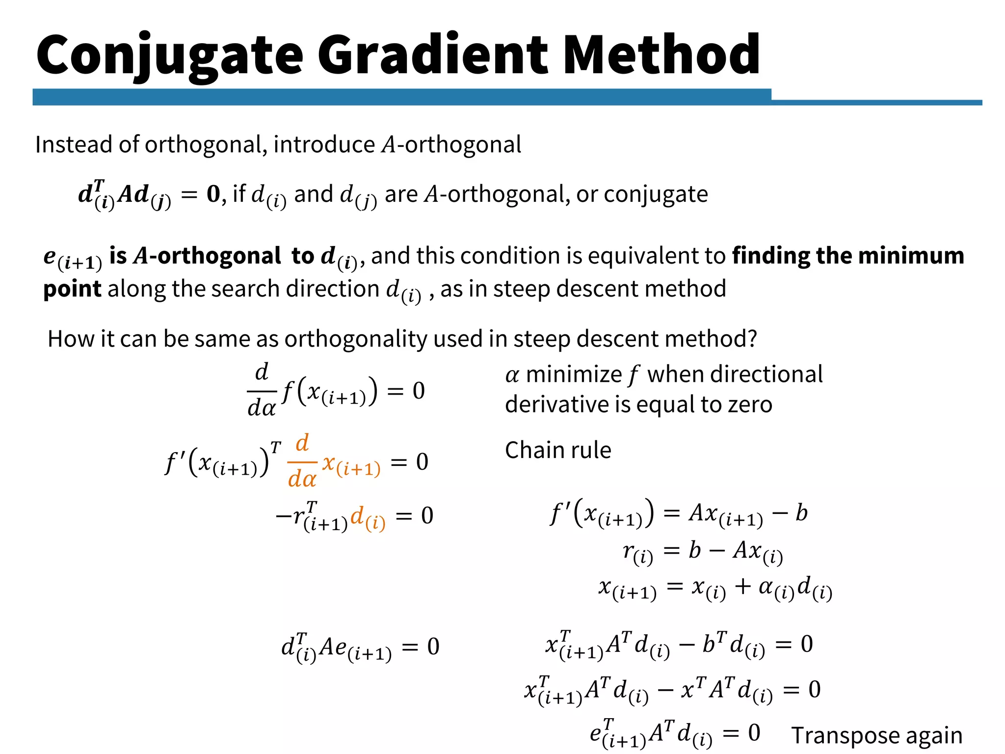
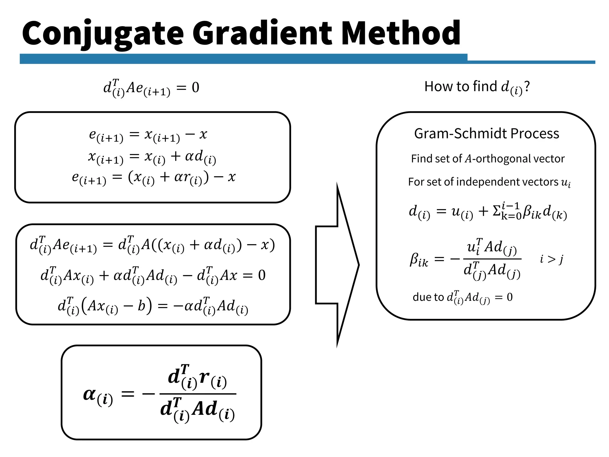
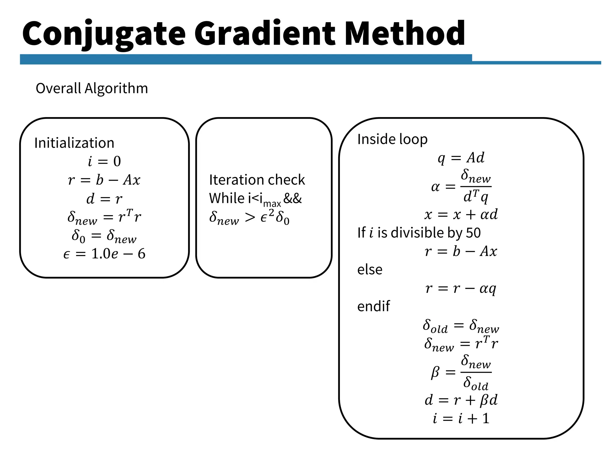
Detailed exploration of the Conjugate Gradient method, its principles, algorithm, and its application in linear systems.
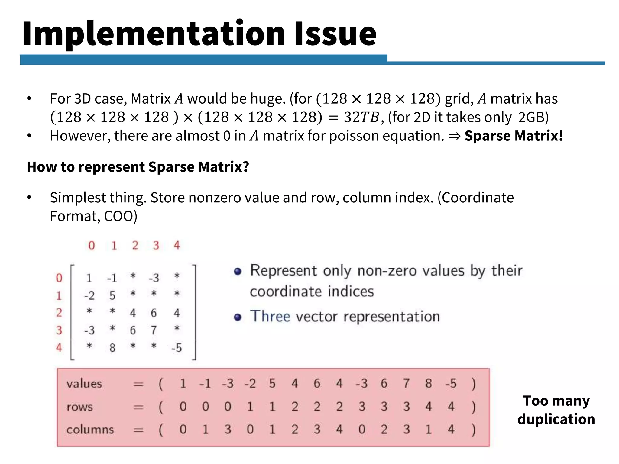
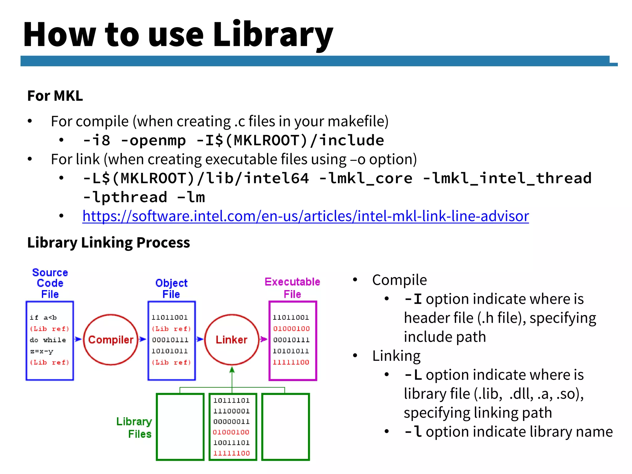
Implementation challenges related to sparse matrices, usage of Intel MKL for efficient computations and linking library processes.


![ANPARA THERMAL POWER STATION[1] sangam.pdf](https://cdn.slidesharecdn.com/ss_thumbnails/anparathermalpowerstation1sangam-251121115219-9261cde4-thumbnail.jpg?width=640&height=640&fit=bounds)


