This document provides an overview of key concepts related to random variables and probability distributions. It discusses:
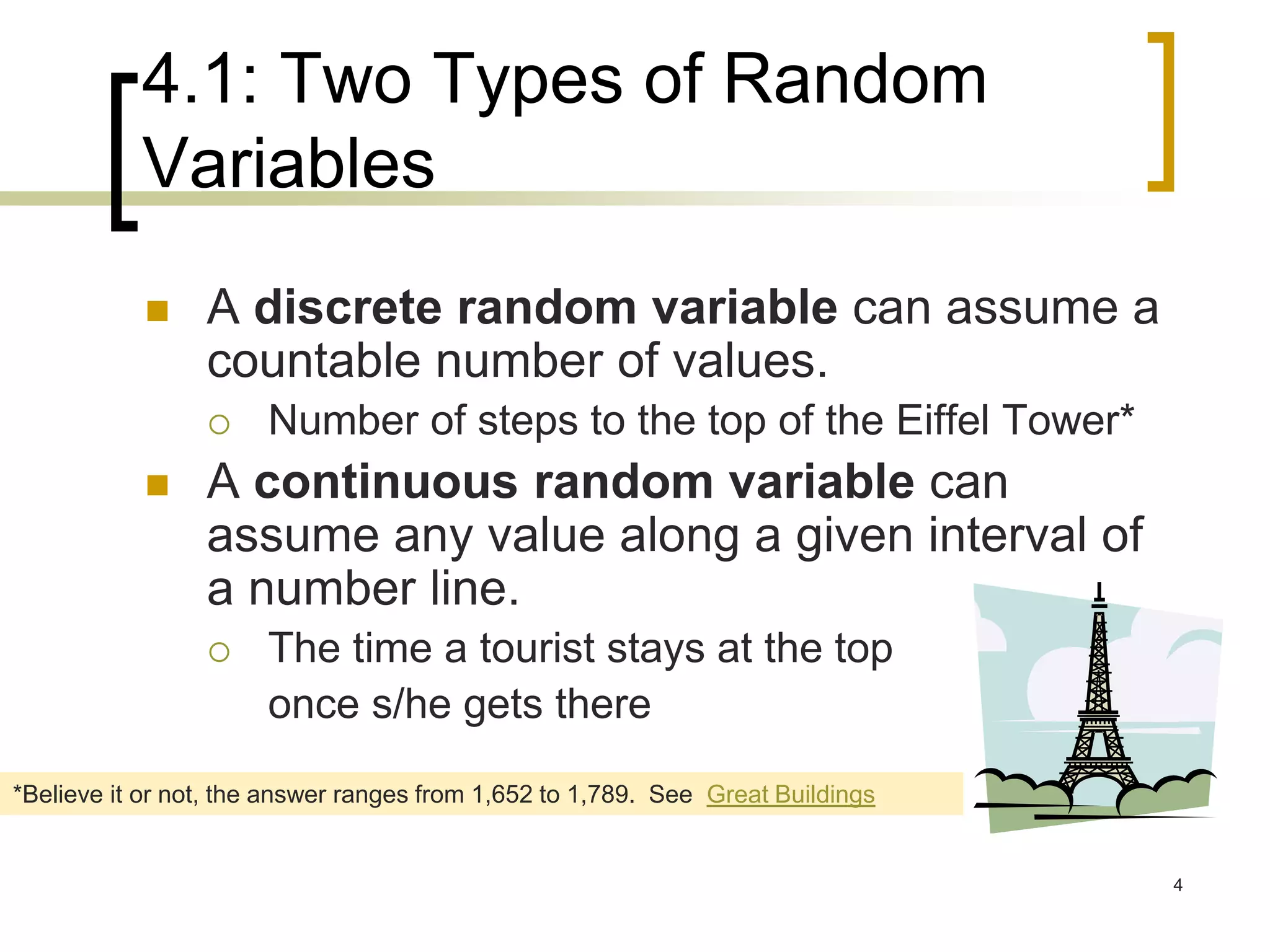
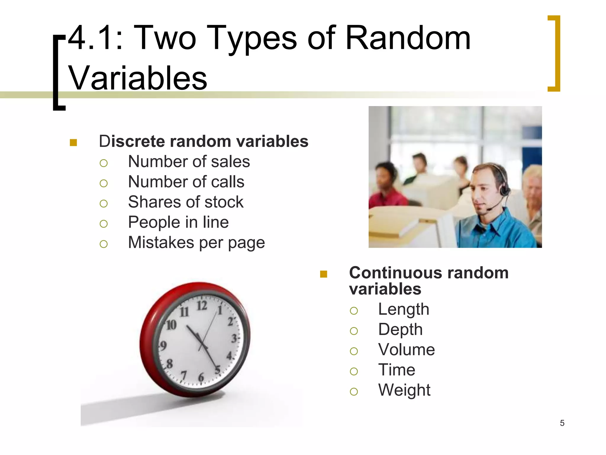
- Two types of random variables - discrete and continuous. Discrete variables can take countable values, continuous can be any value in an interval.
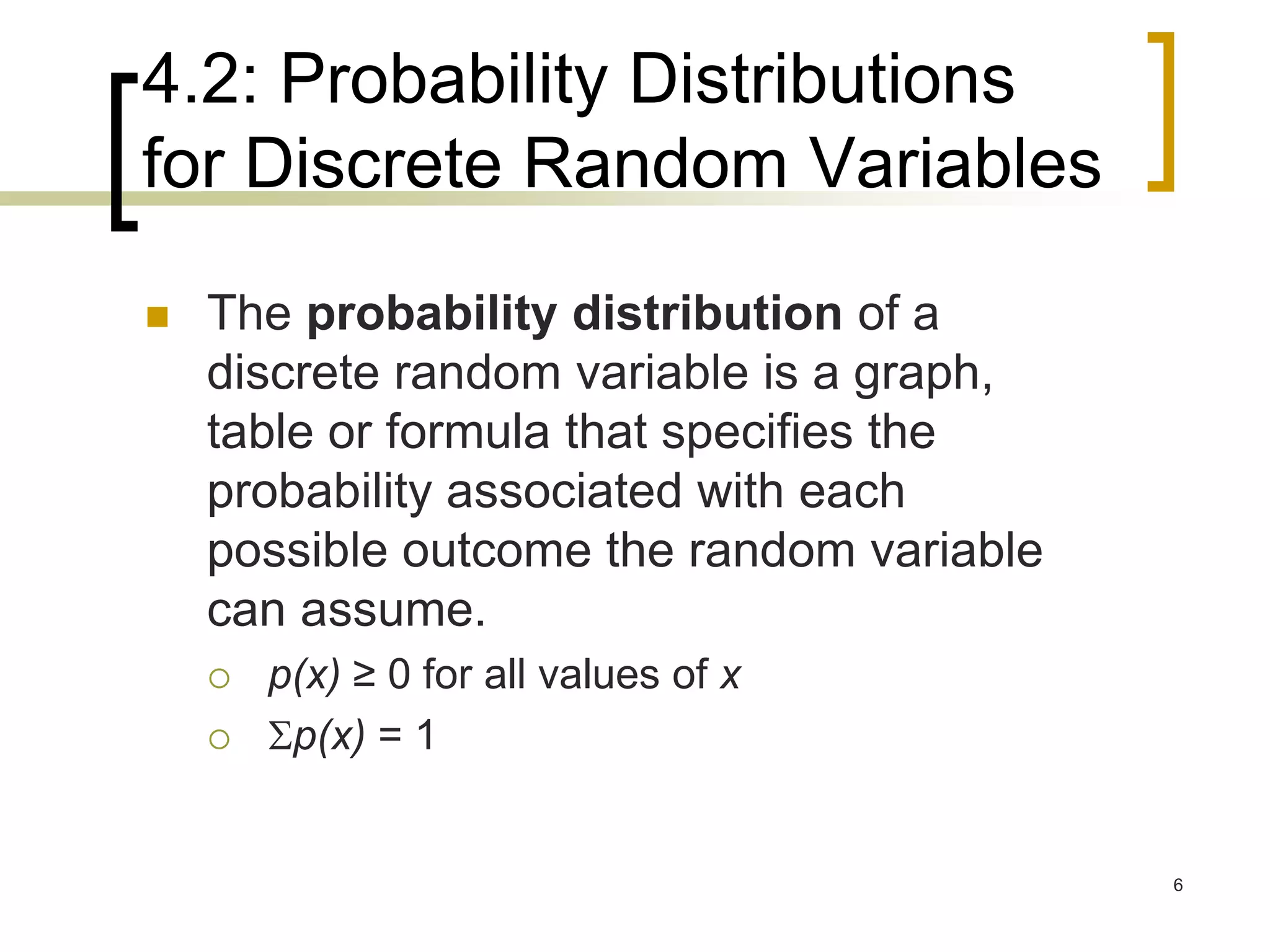
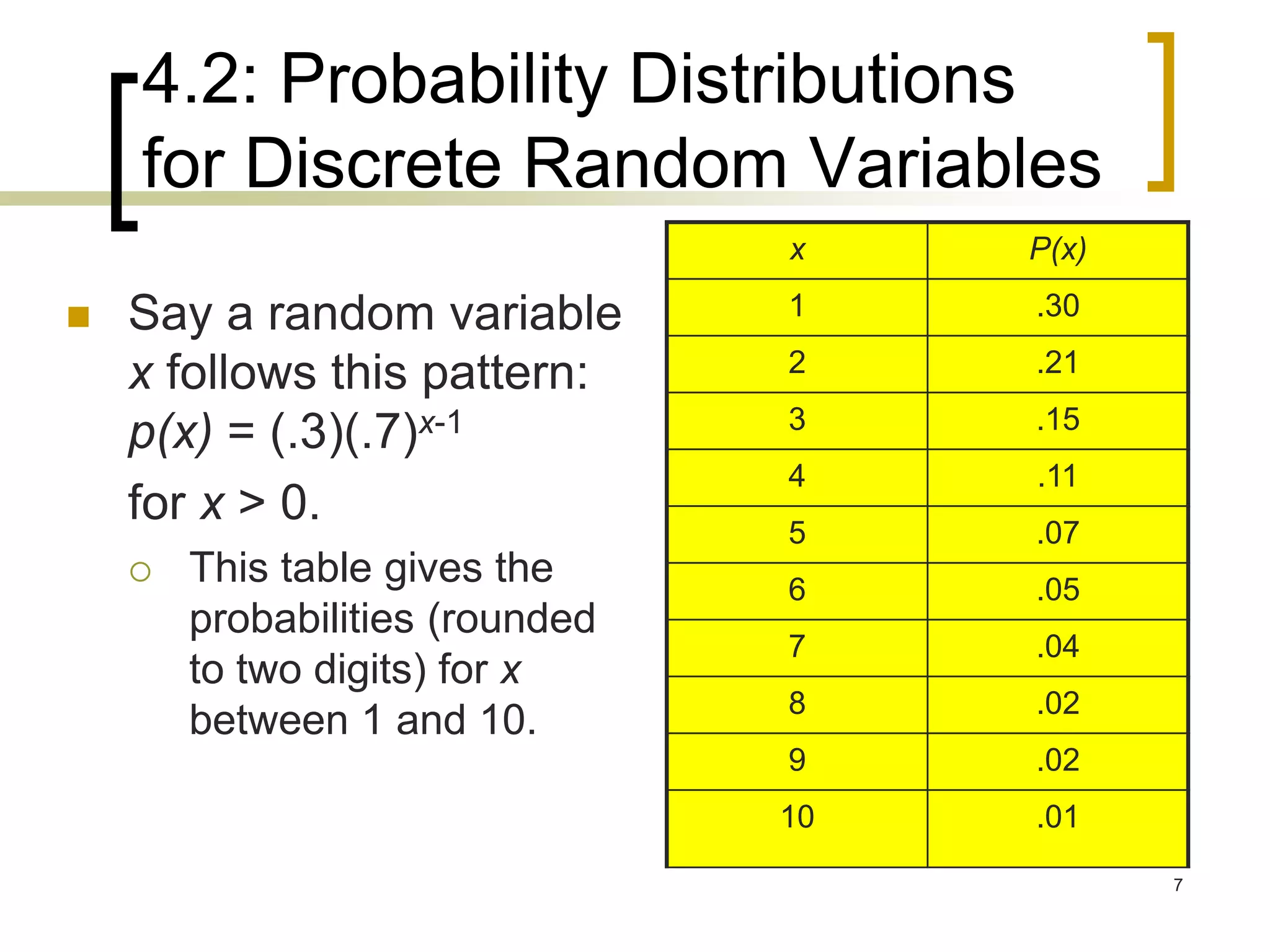
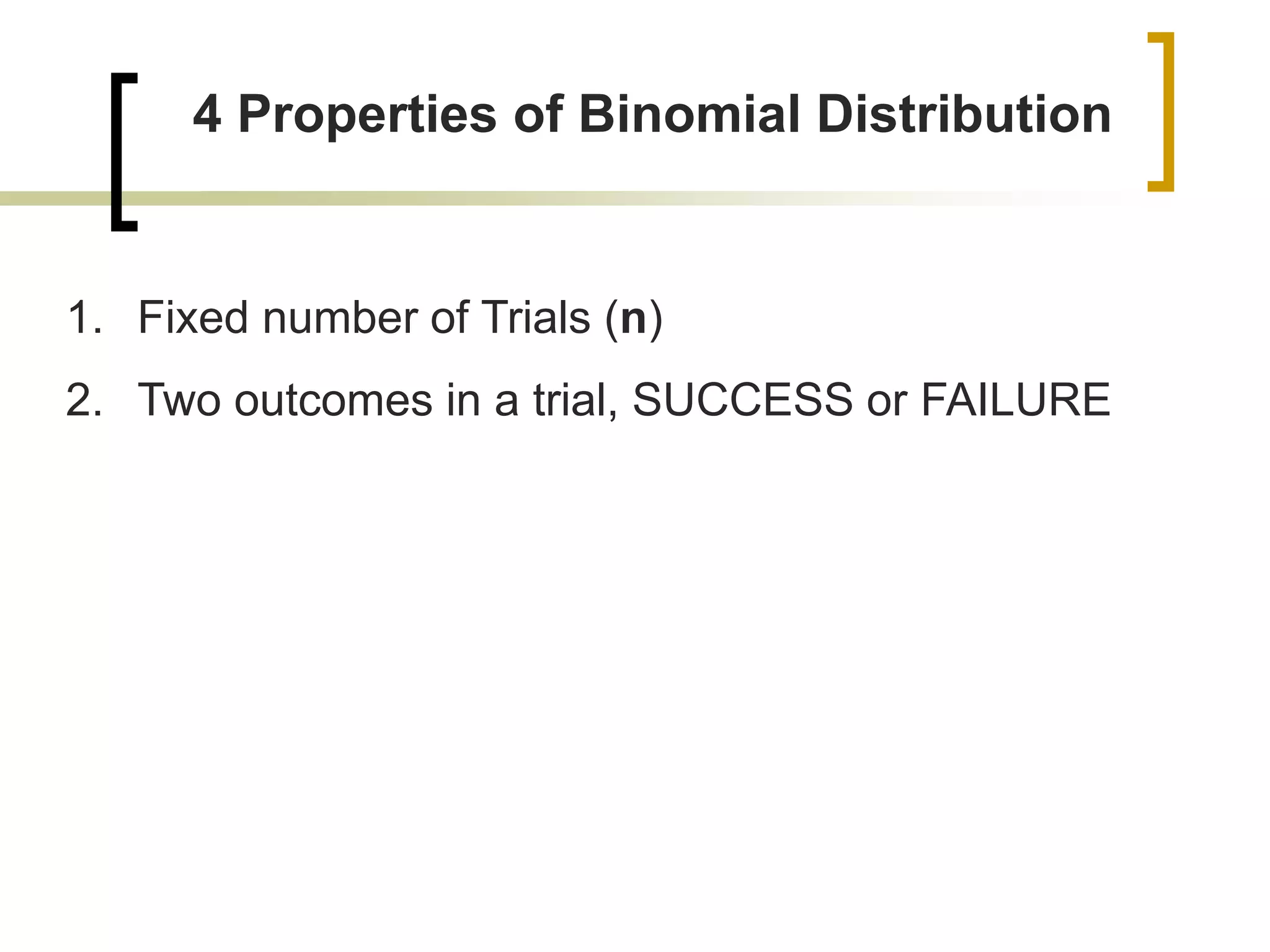
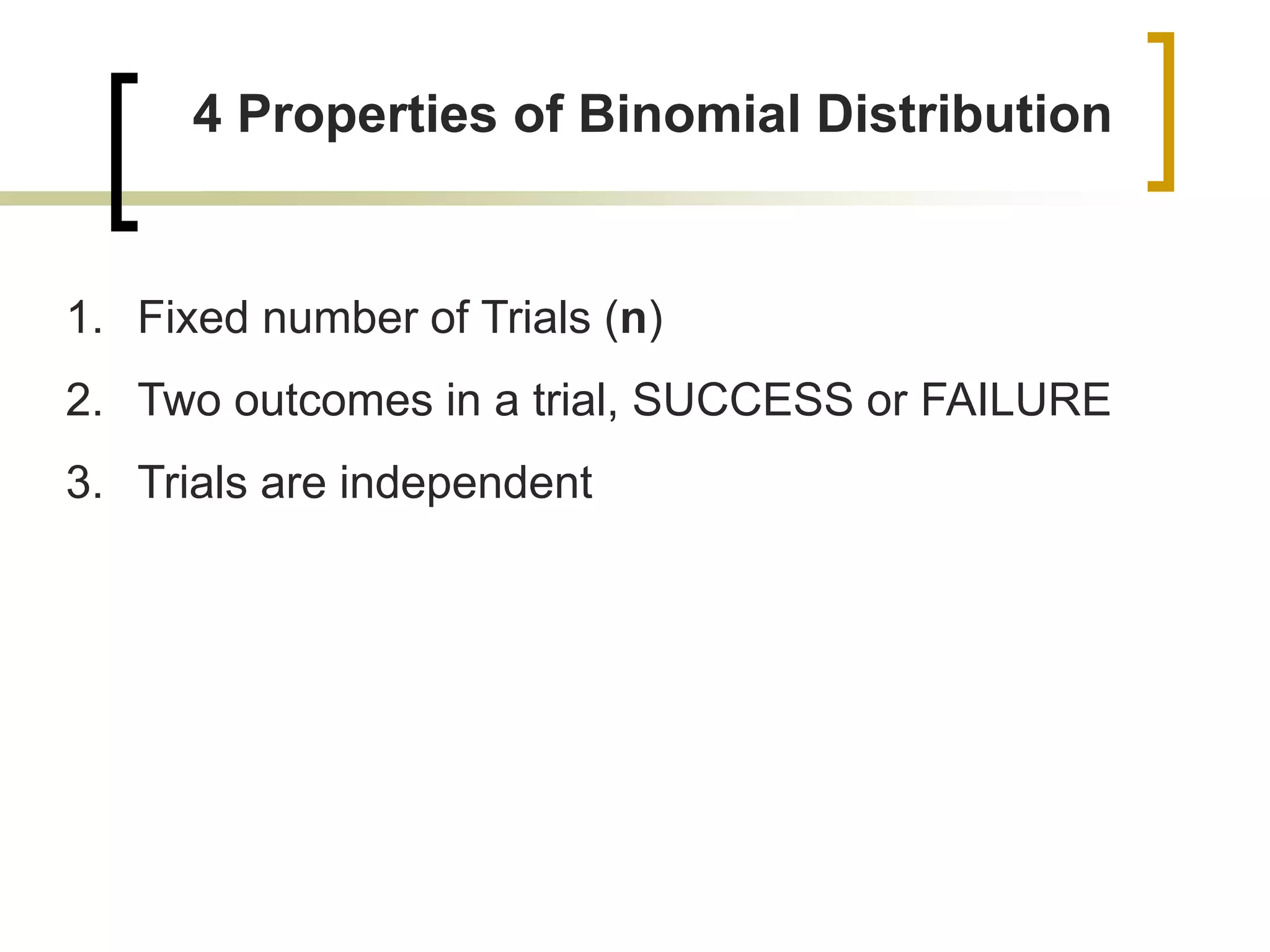
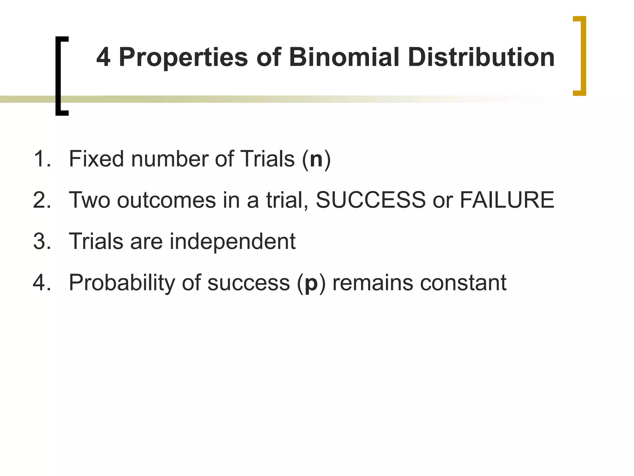
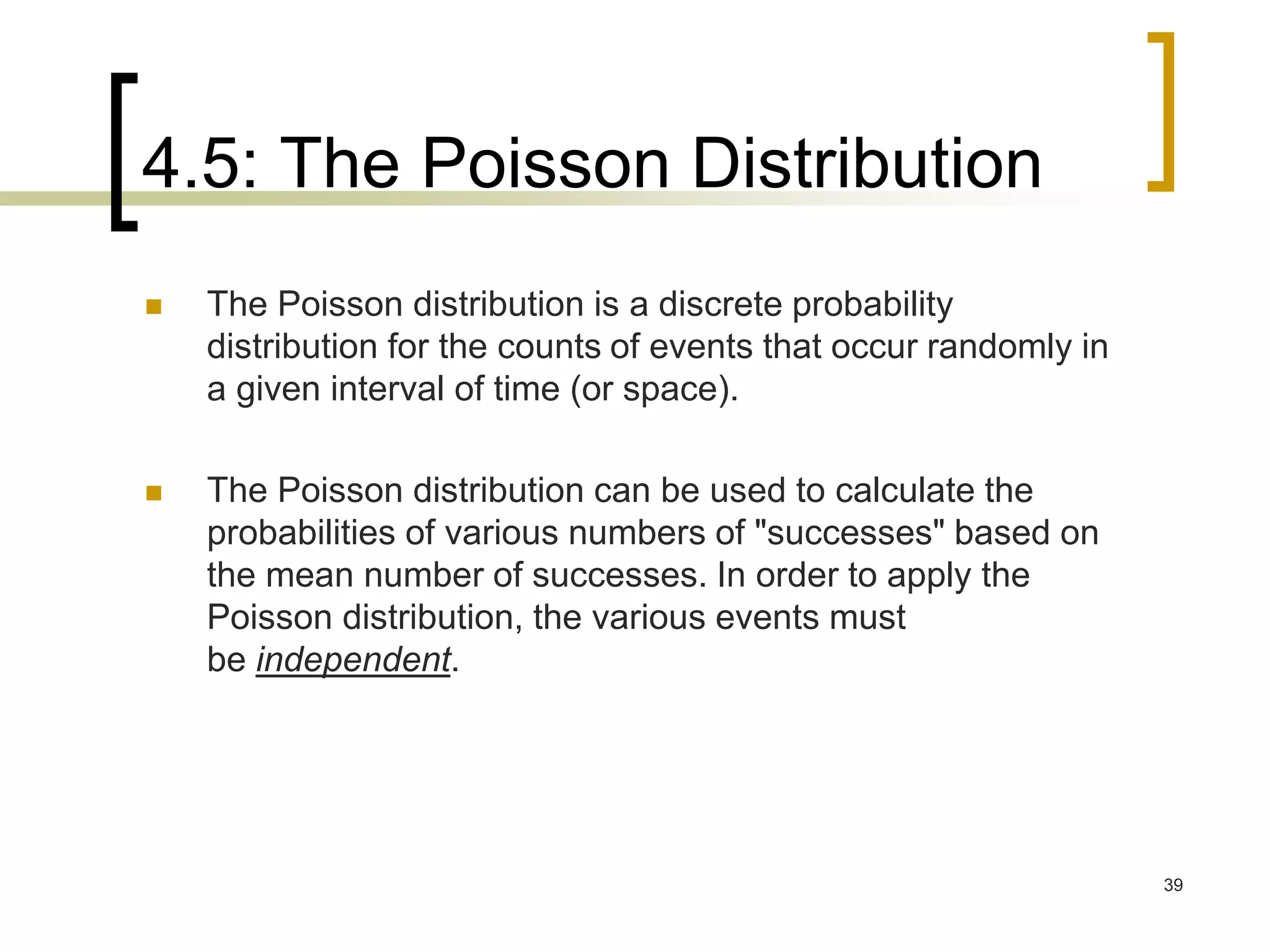
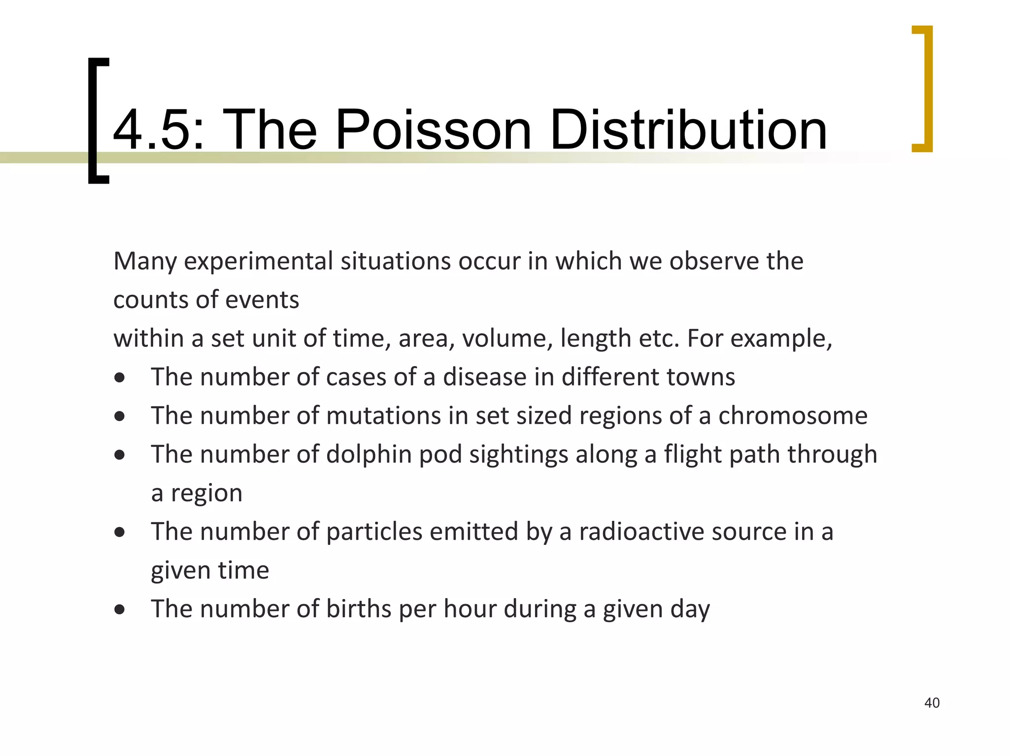
- Probability distributions for discrete random variables, which specify the probability of each possible outcome. Examples of common discrete distributions like binomial and Poisson are provided.
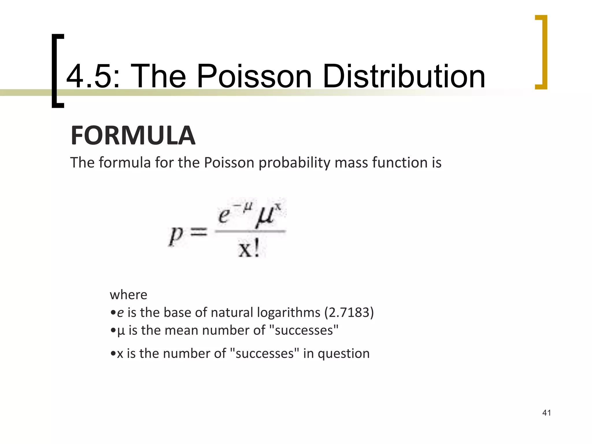
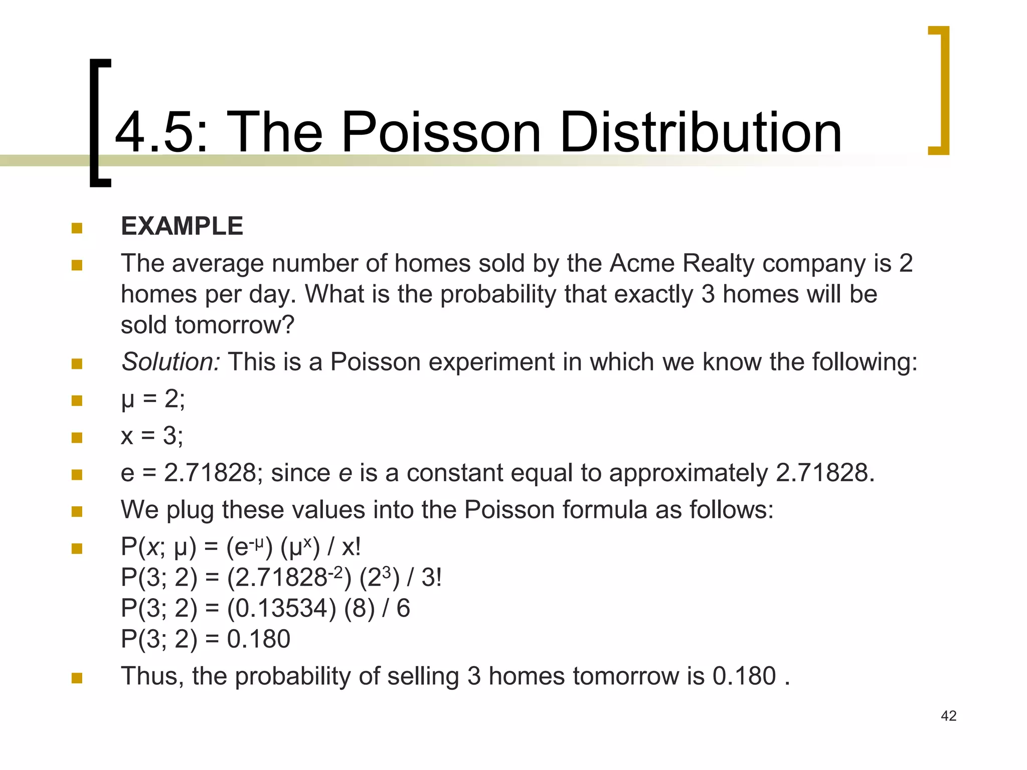
- Key properties and calculations for discrete distributions like expected value, variance, and the formulas for binomial and Poisson probabilities.
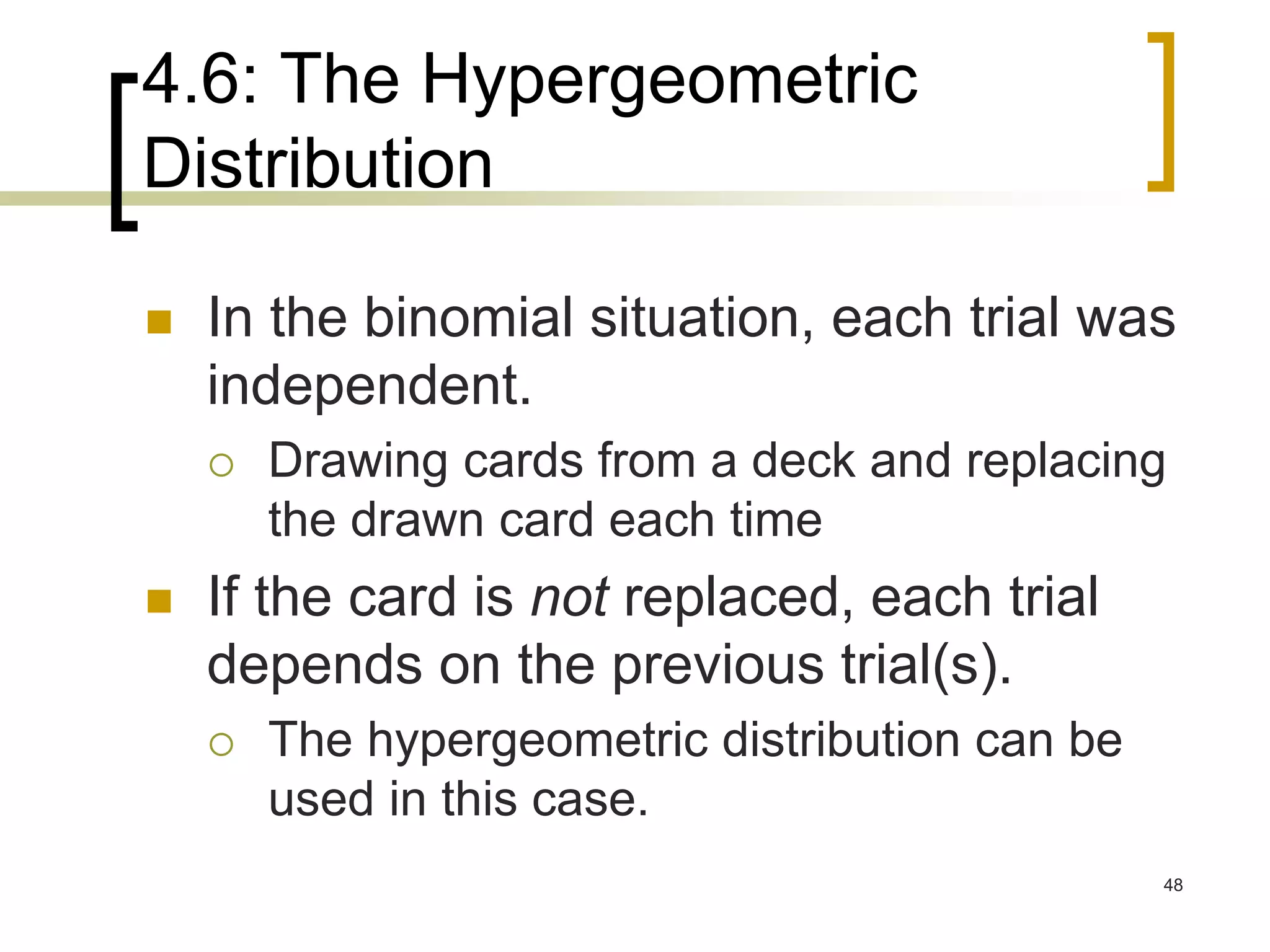
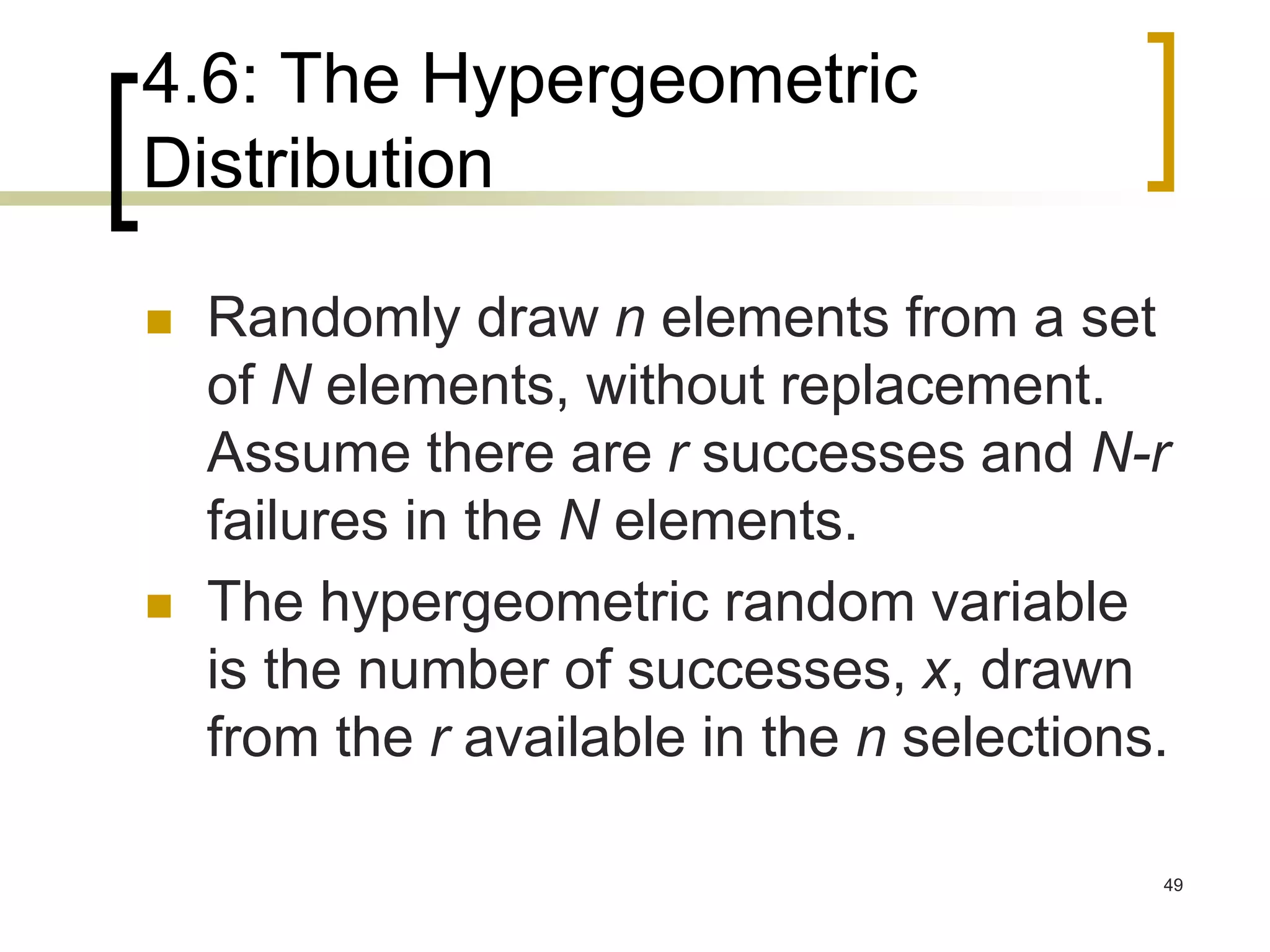
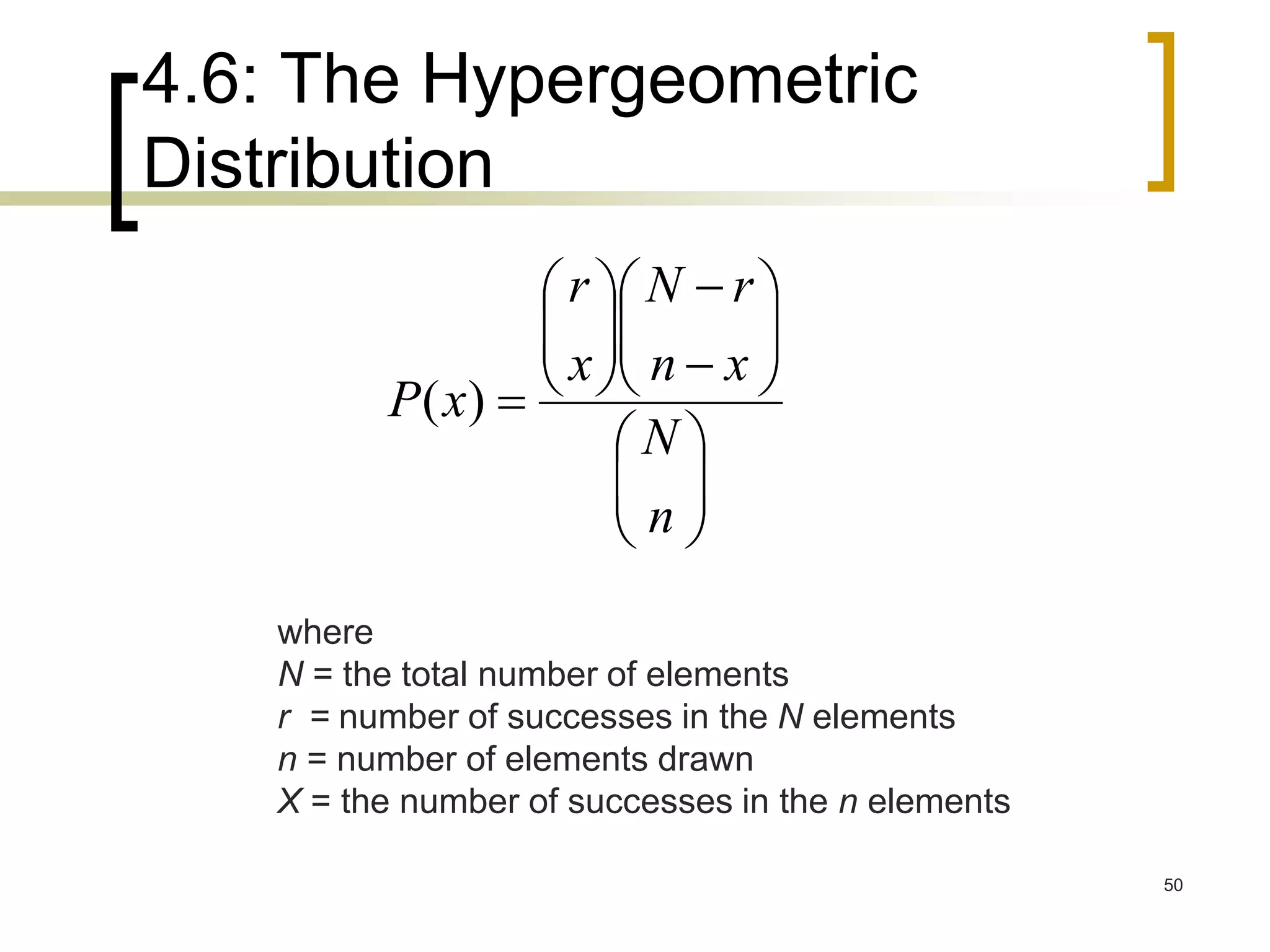
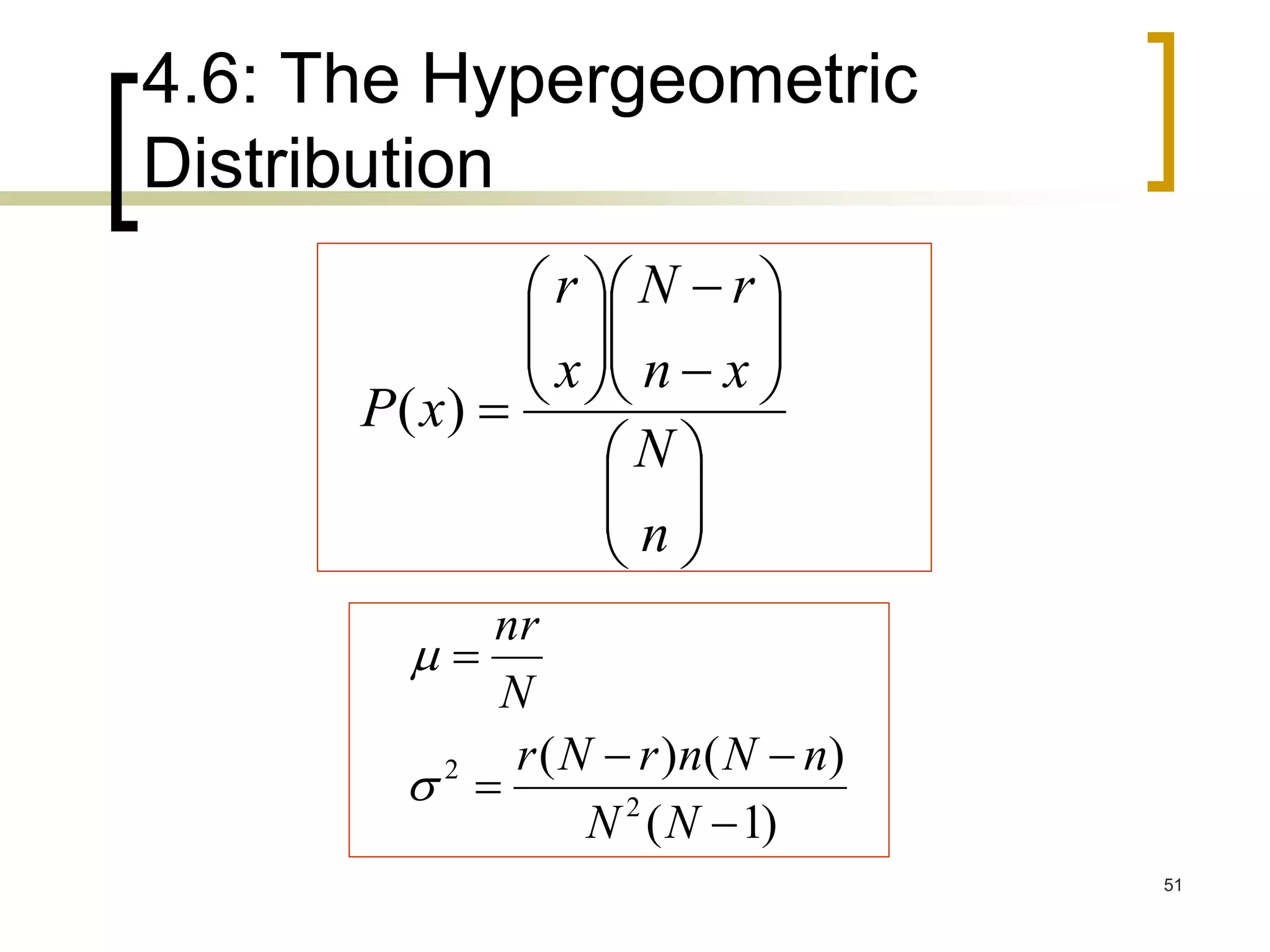
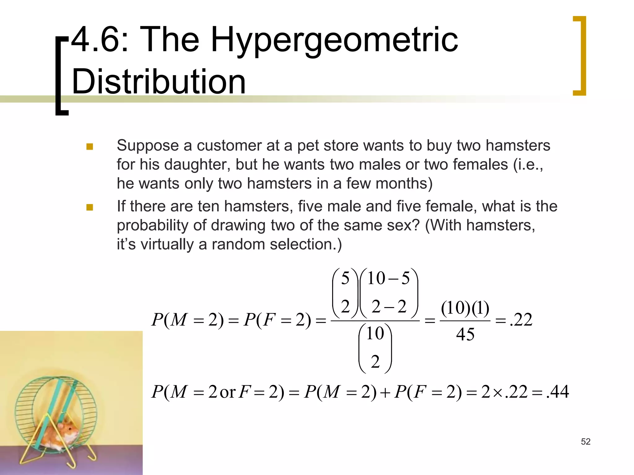
- Other discrete distributions like hypergeometric are introduced for situations where outcomes are not independent. Examples are provided to demonstrate calculating probabilities for each type of distribution.

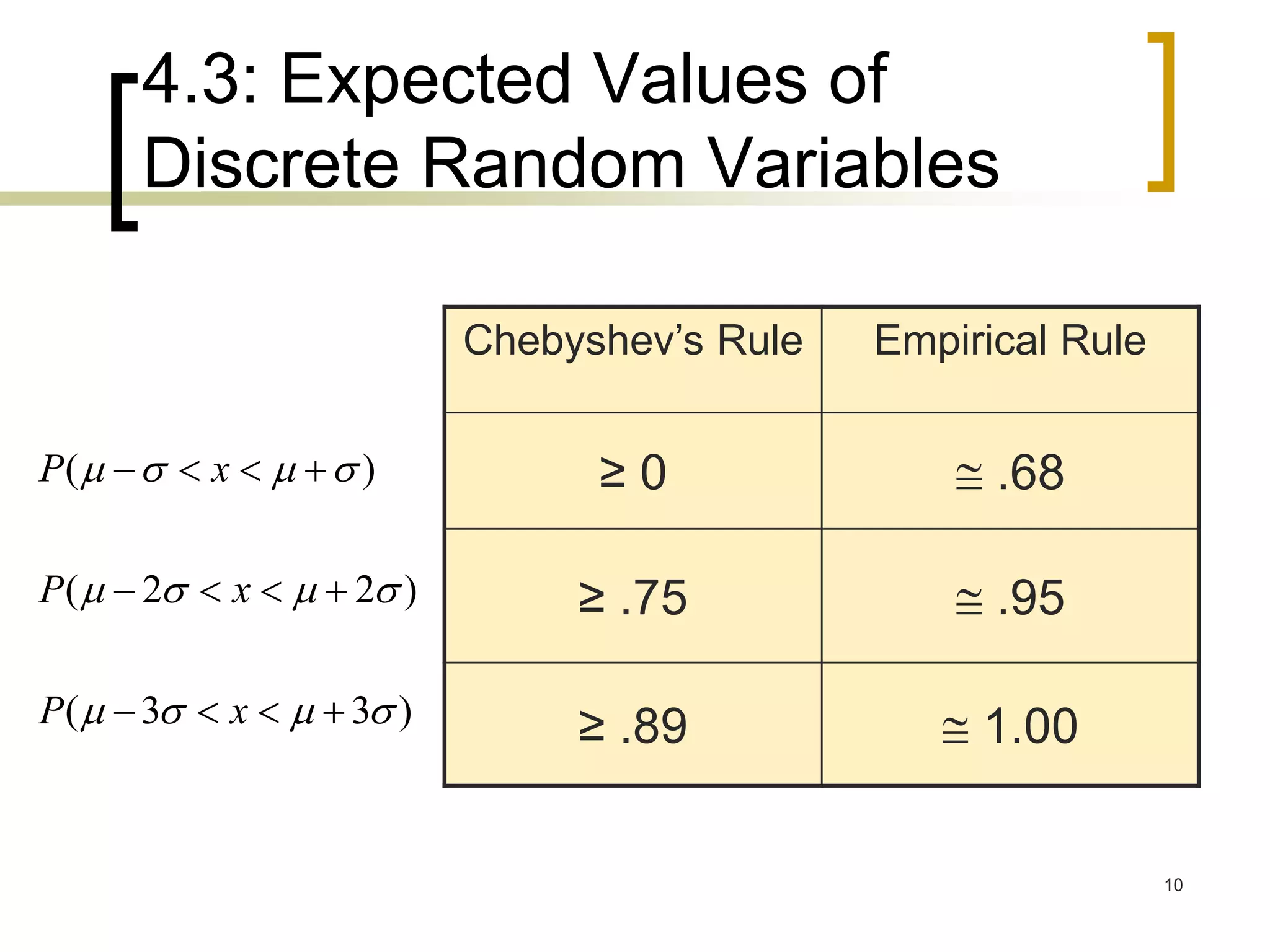
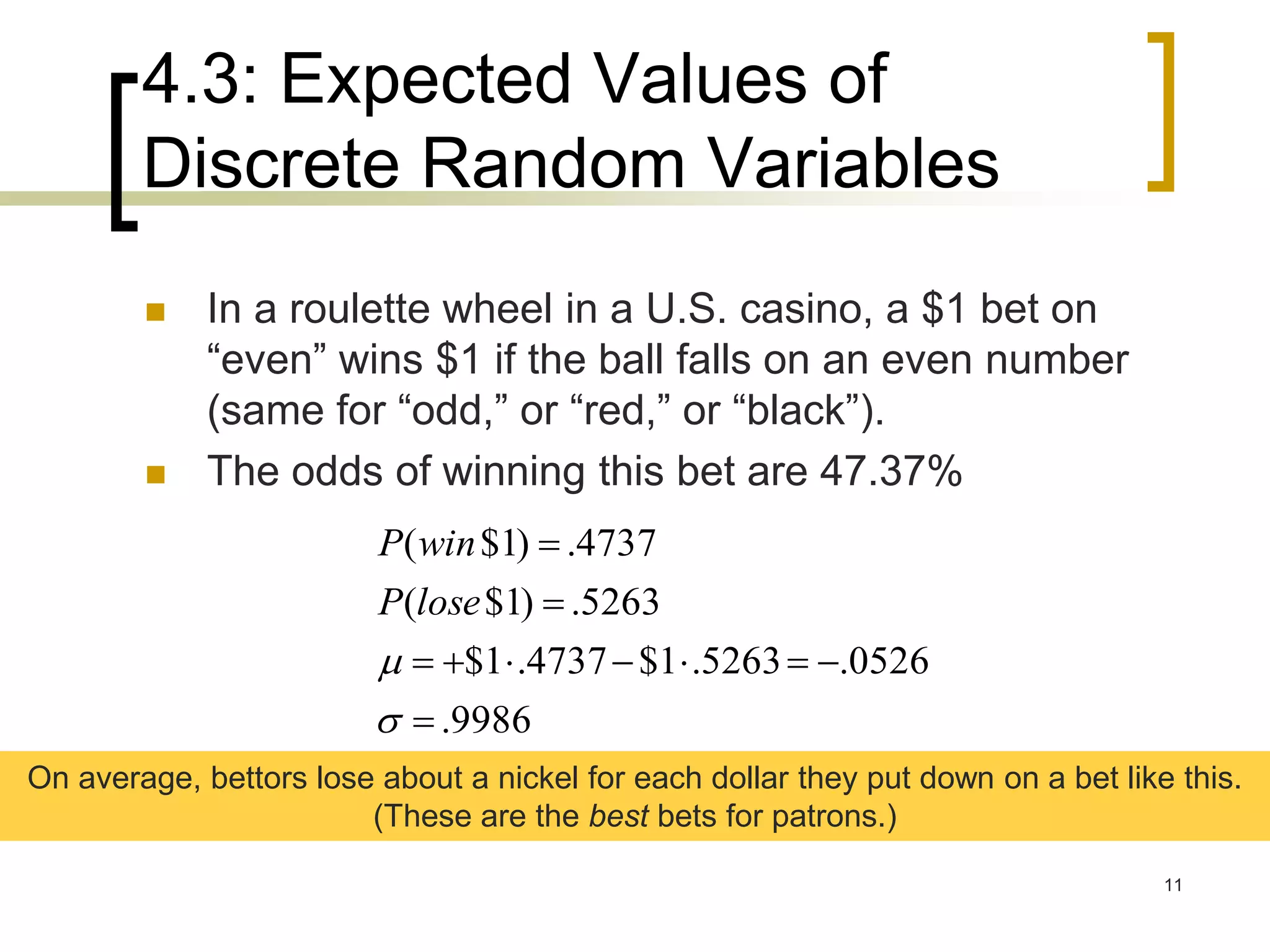
![4.3: Expected Values of
Discrete Random Variables
The variance of a discrete random
variable x is
The standard deviation of a discrete
random variable x is
2 2 2
[( ) ] ( ) ( ).E x x p x
2 2 2
[( ) ] ( ) ( ).E x x p x
9](https://image.slidesharecdn.com/group4-randomvariableanddistribution-151014015655-lva1-app6891/75/random-variable-and-distribution-9-2048.jpg)


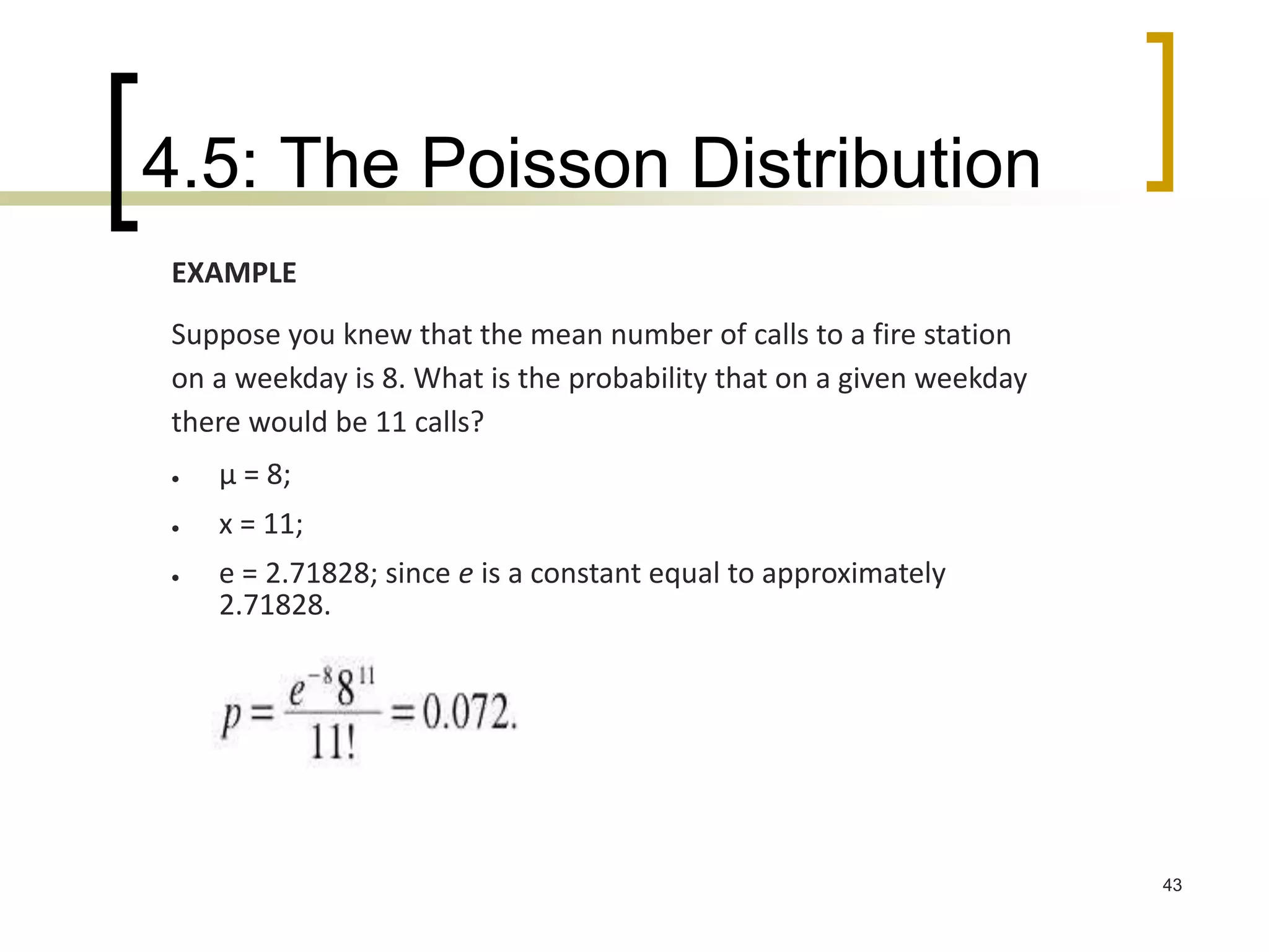
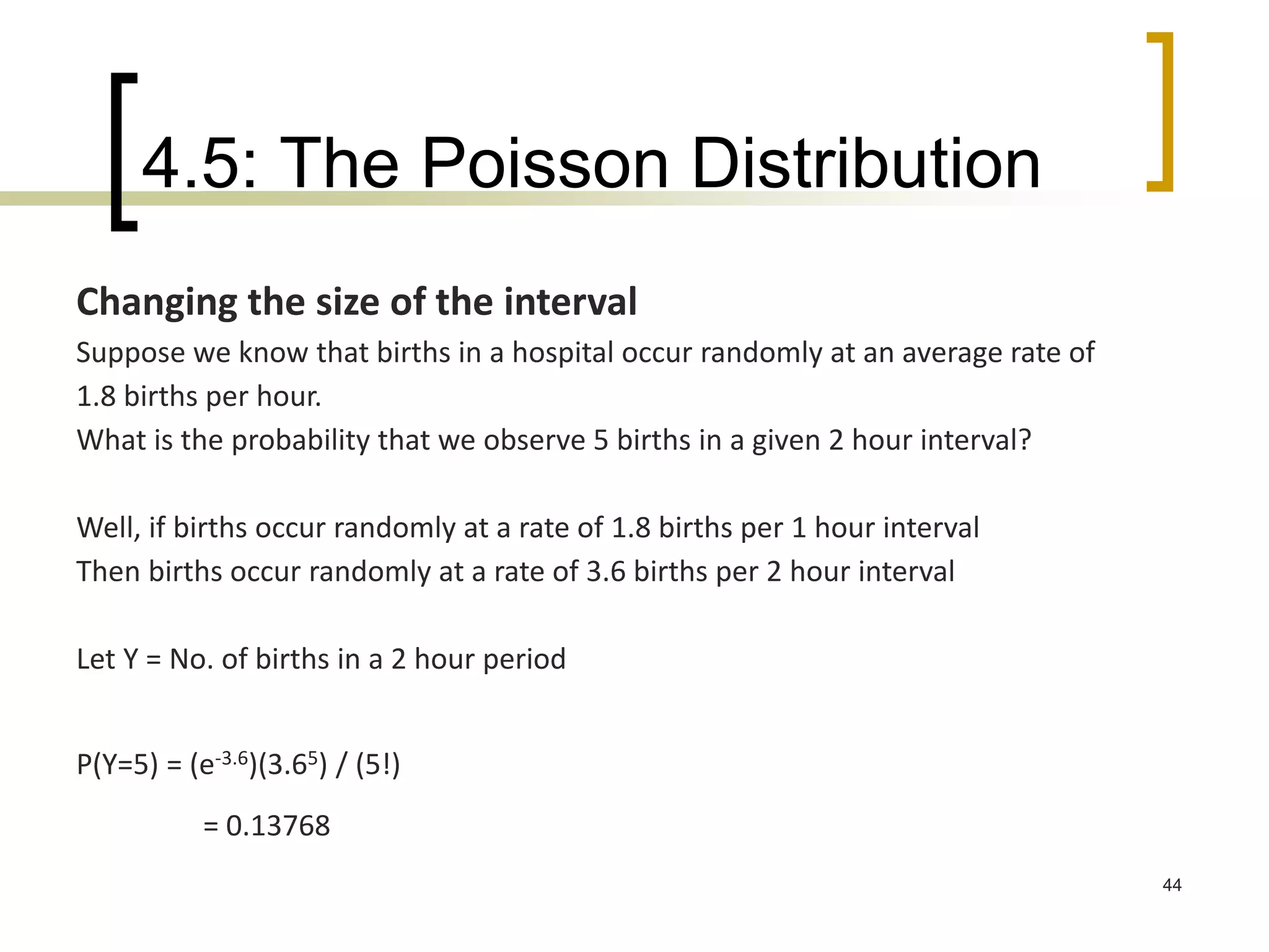
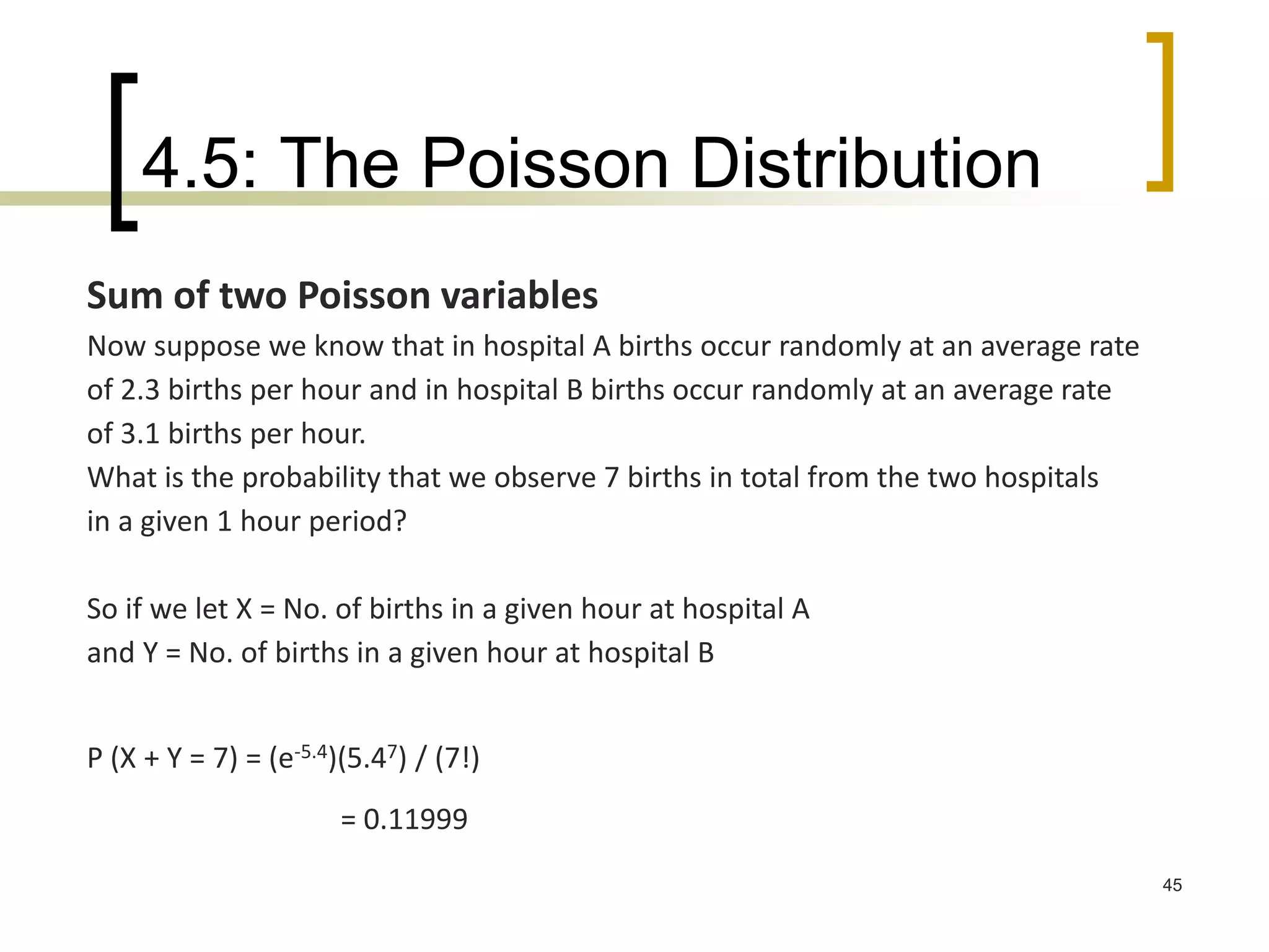
![4.5: The Poisson Distribution
47
Example 1
een on a 1-day safari is 5. What is the probability that tourists will
see fewer than four lions on the next 1-day safari?
Solution: This is a Poisson experiment in
Suppose the average number of lions s which we know the
following:
μ = 5;
x = 0, 1, 2, or 3;
e = 2.71828; since e is a constant equal to approximately
2.71828.
To solve this problem, we need to find the probability that tourists will see
0, 1, 2, or 3 lions. Thus, we need to calculate the sum of four probabilities:
P(0; 5) + P(1; 5) + P(2; 5) + P(3; 5). To compute this sum, we use the Poisson
formula:
P(x < 3, 5) = P(0; 5) + P(1; 5) + P(2; 5) + P(3; 5)
P(x < 3, 5) = [ (e-5)(50) / 0! ] + [ (e-5)(51) / 1! ] + [ (e-5)(52) / 2! ] + [ (e-5)(53) / 3!
]
P(x < 3, 5) = [ (0.006738)(1) / 1 ] + [ (0.006738)(5) / 1 ] + [ (0.006738)(25) / 2
] + [ (0.006738)(125) / 6 ]
P(x < 3, 5) = [ 0.0067 ] + [ 0.03369 ] + [ 0.084224 ] + [ 0.140375 ]
P(x < 3, 5) = 0.2650
Thus, the probability of seeing at no more than 3 lions is 0.2650.](https://image.slidesharecdn.com/group4-randomvariableanddistribution-151014015655-lva1-app6891/75/random-variable-and-distribution-47-2048.jpg)


![4.3: Expected Values of
Discrete Random Variables
The variance of a discrete random
variable x is
The standard deviation of a discrete
random variable x is
2 2 2
[( ) ] ( ) ( ).E x x p x
2 2 2
[( ) ] ( ) ( ).E x x p x
9](https://crownmelresort.com/image.slidesharecdn.com/group4-randomvariableanddistribution-151014015655-lva1-app6891/75/random-variable-and-distribution-9-2048.jpg)


![4.5: The Poisson Distribution
47
Example 1
een on a 1-day safari is 5. What is the probability that tourists will
see fewer than four lions on the next 1-day safari?
Solution: This is a Poisson experiment in
Suppose the average number of lions s which we know the
following:
μ = 5;
x = 0, 1, 2, or 3;
e = 2.71828; since e is a constant equal to approximately
2.71828.
To solve this problem, we need to find the probability that tourists will see
0, 1, 2, or 3 lions. Thus, we need to calculate the sum of four probabilities:
P(0; 5) + P(1; 5) + P(2; 5) + P(3; 5). To compute this sum, we use the Poisson
formula:
P(x < 3, 5) = P(0; 5) + P(1; 5) + P(2; 5) + P(3; 5)
P(x < 3, 5) = [ (e-5)(50) / 0! ] + [ (e-5)(51) / 1! ] + [ (e-5)(52) / 2! ] + [ (e-5)(53) / 3!
]
P(x < 3, 5) = [ (0.006738)(1) / 1 ] + [ (0.006738)(5) / 1 ] + [ (0.006738)(25) / 2
] + [ (0.006738)(125) / 6 ]
P(x < 3, 5) = [ 0.0067 ] + [ 0.03369 ] + [ 0.084224 ] + [ 0.140375 ]
P(x < 3, 5) = 0.2650
Thus, the probability of seeing at no more than 3 lions is 0.2650.](https://crownmelresort.com/image.slidesharecdn.com/group4-randomvariableanddistribution-151014015655-lva1-app6891/75/random-variable-and-distribution-47-2048.jpg)


![ANPARA THERMAL POWER STATION[1] sangam.pdf](https://cdn.slidesharecdn.com/ss_thumbnails/anparathermalpowerstation1sangam-251121115219-9261cde4-thumbnail.jpg?width=640&height=640&fit=bounds)


