Downloaded 149 times


The document discusses the definitions and key concepts of random variables in probability theory, distinguishing between discrete and continuous random variables. It explains that discrete random variables take a finite or countable number of values, while continuous random variables can assume any value within a certain interval. Additionally, the document introduces probability mass functions for discrete variables and probability density functions for continuous variables, along with related concepts such as distribution functions.
Introduction of random variables by Bipul Kumar Sarker, focusing on definitions and chapters.
Defining random variables and the two types: discrete and continuous, crucial for probability theory.
Explaining discrete random variables, emphasizing countable values with an example involving coin toss.
Defining continuous random variables using real-world examples like heights and bulb lifespans.
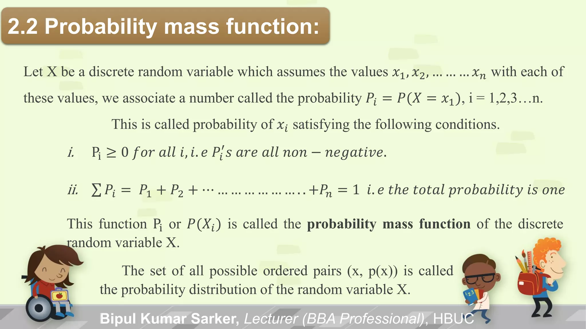
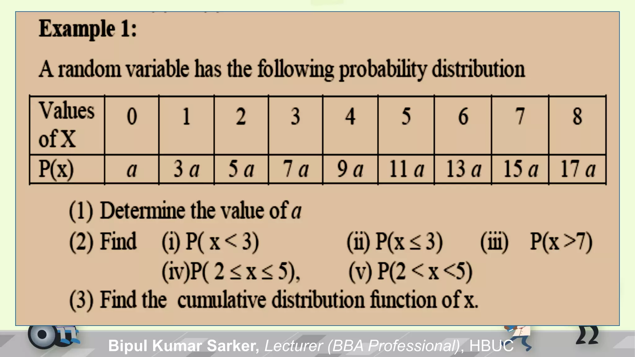
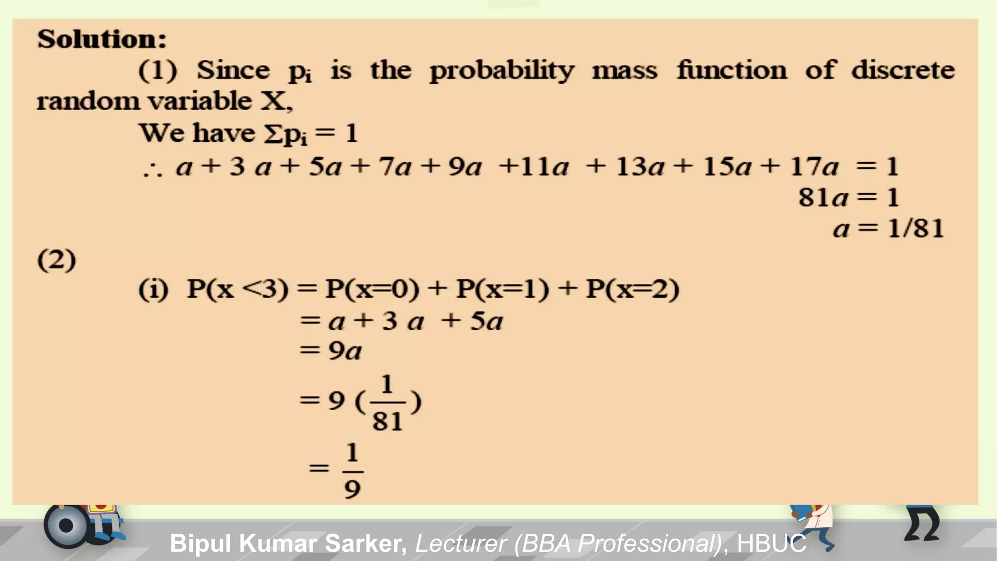
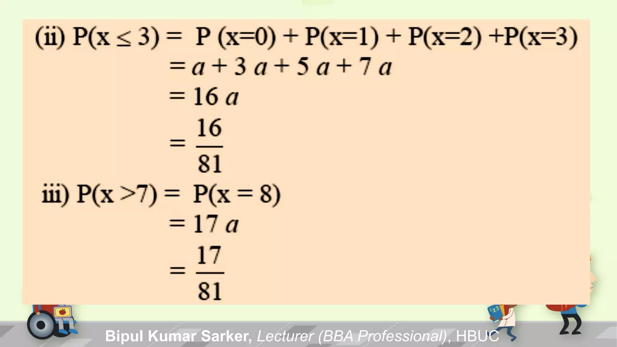
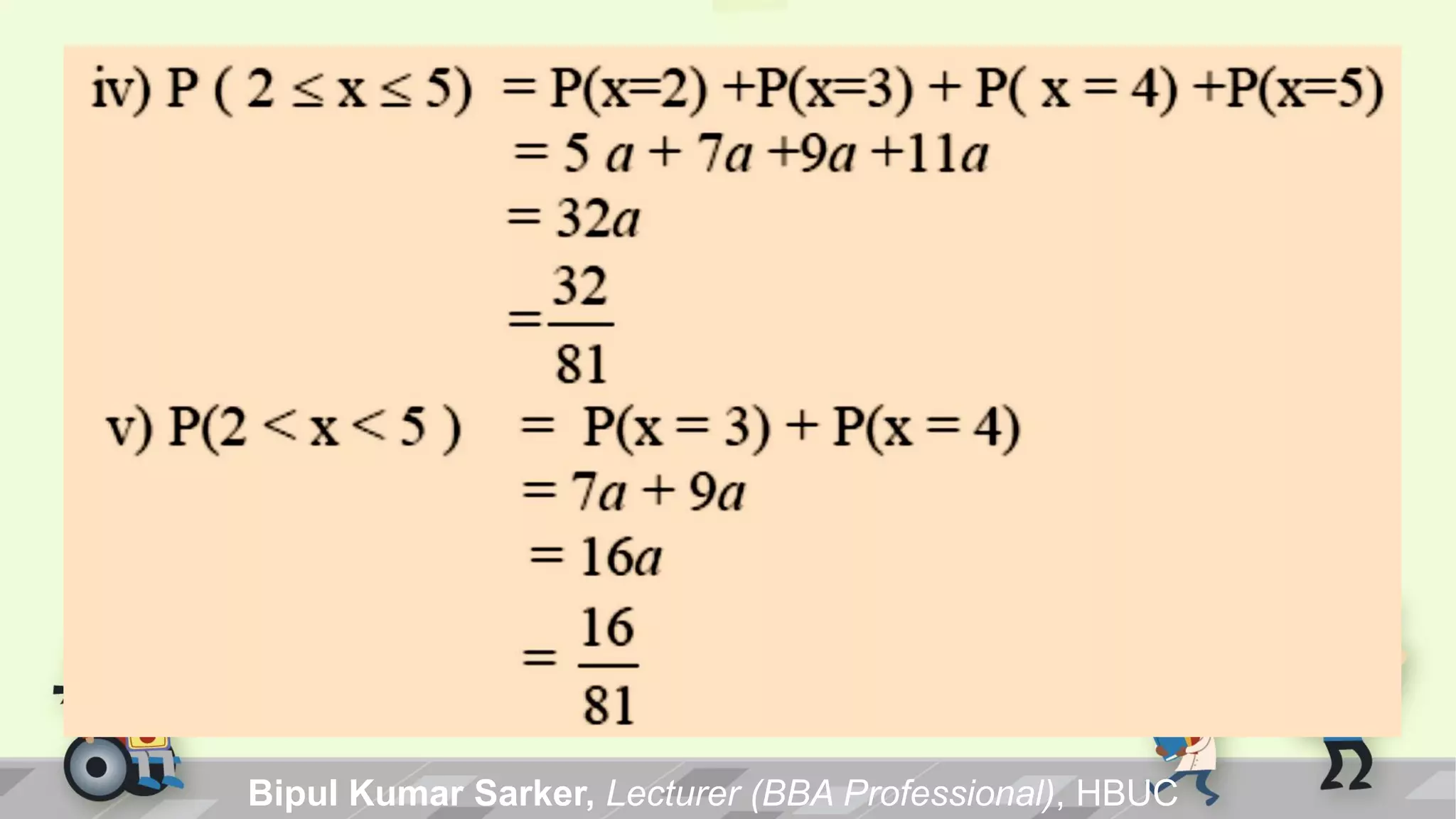
Details on the probability mass function for discrete random variables and its key properties.
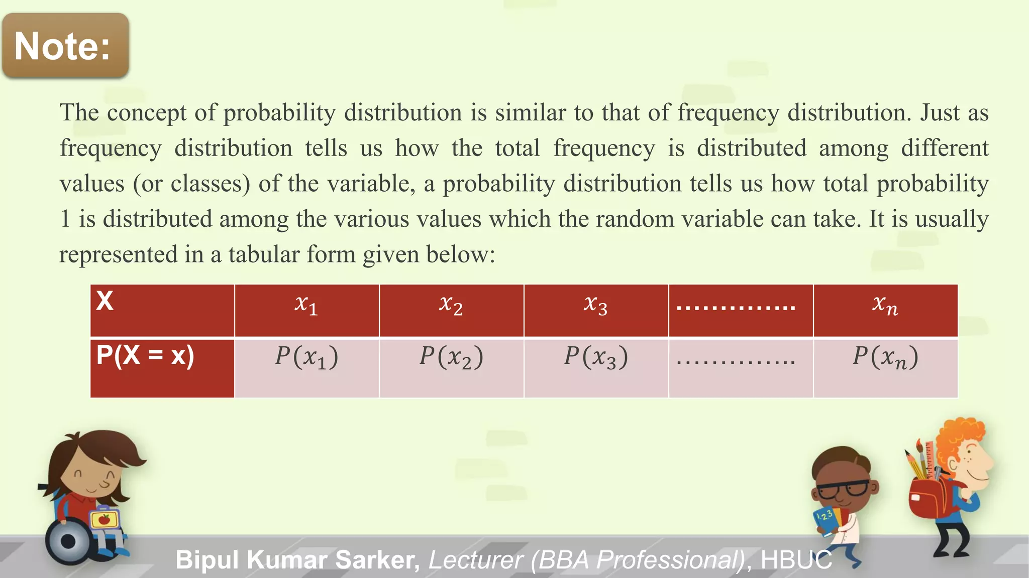
Comparison of probability distribution to frequency distribution, presented in a tabular form.
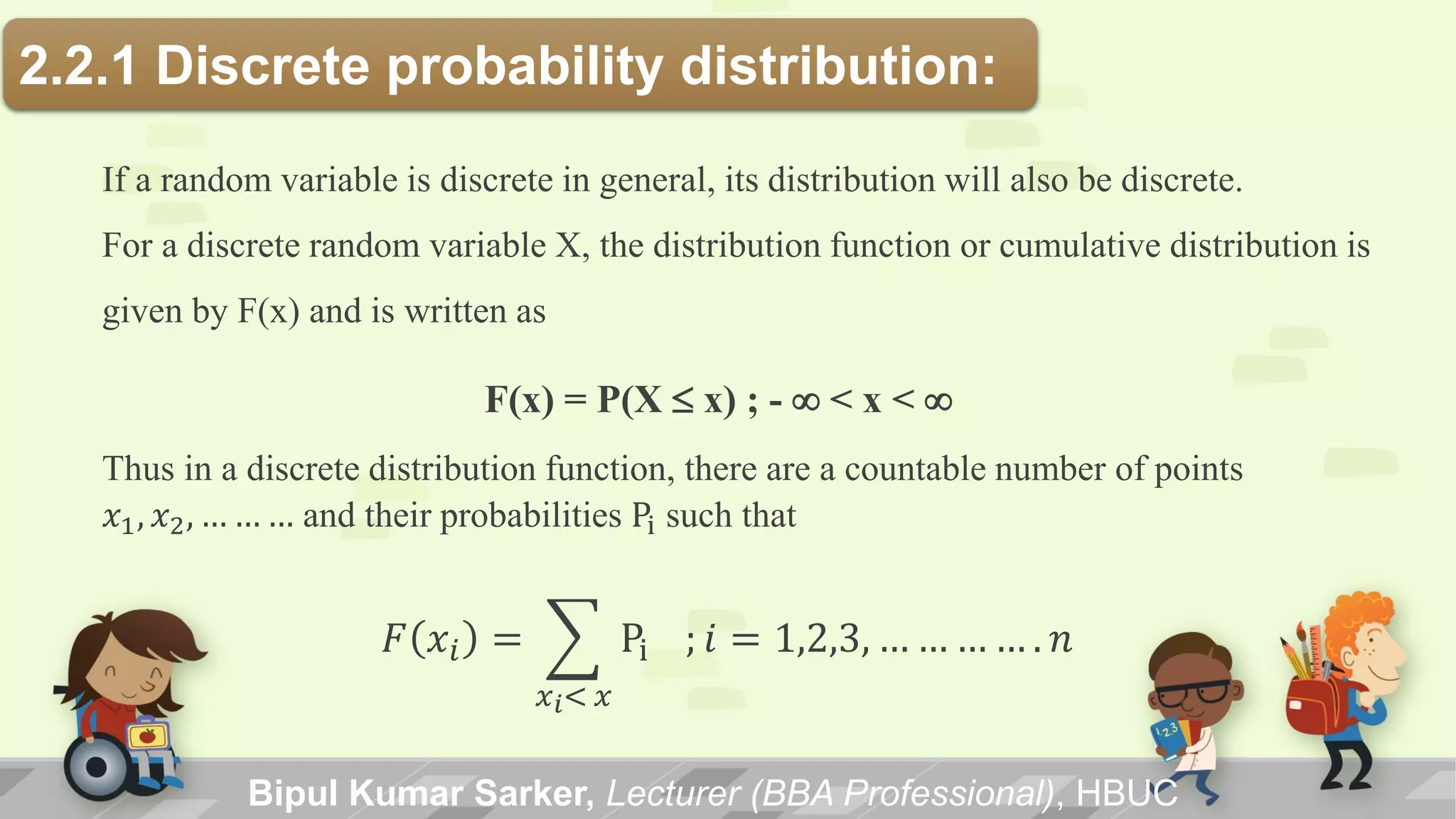
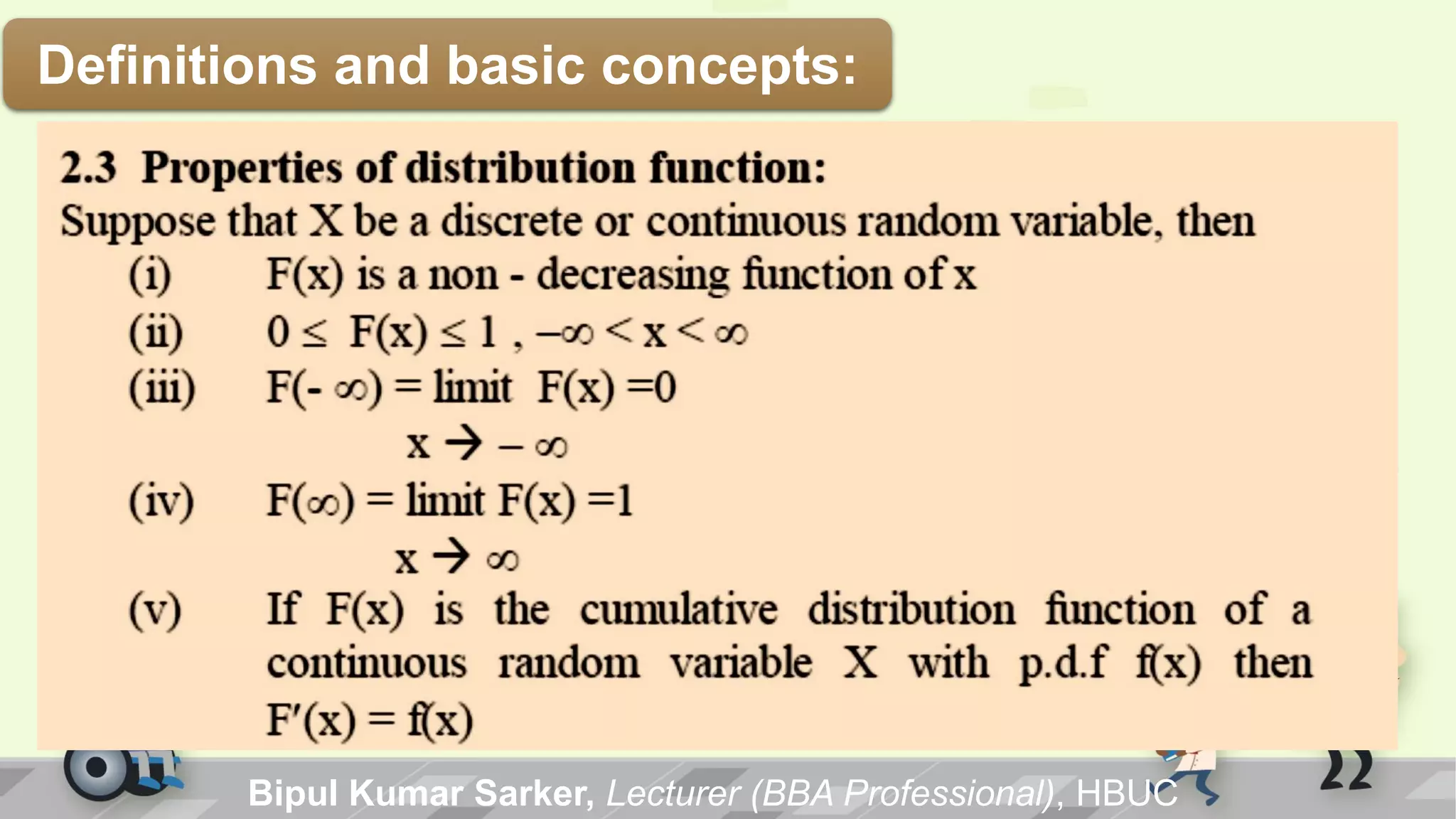
Definition of discrete probability distribution functions and cumulative distribution in probabilities.
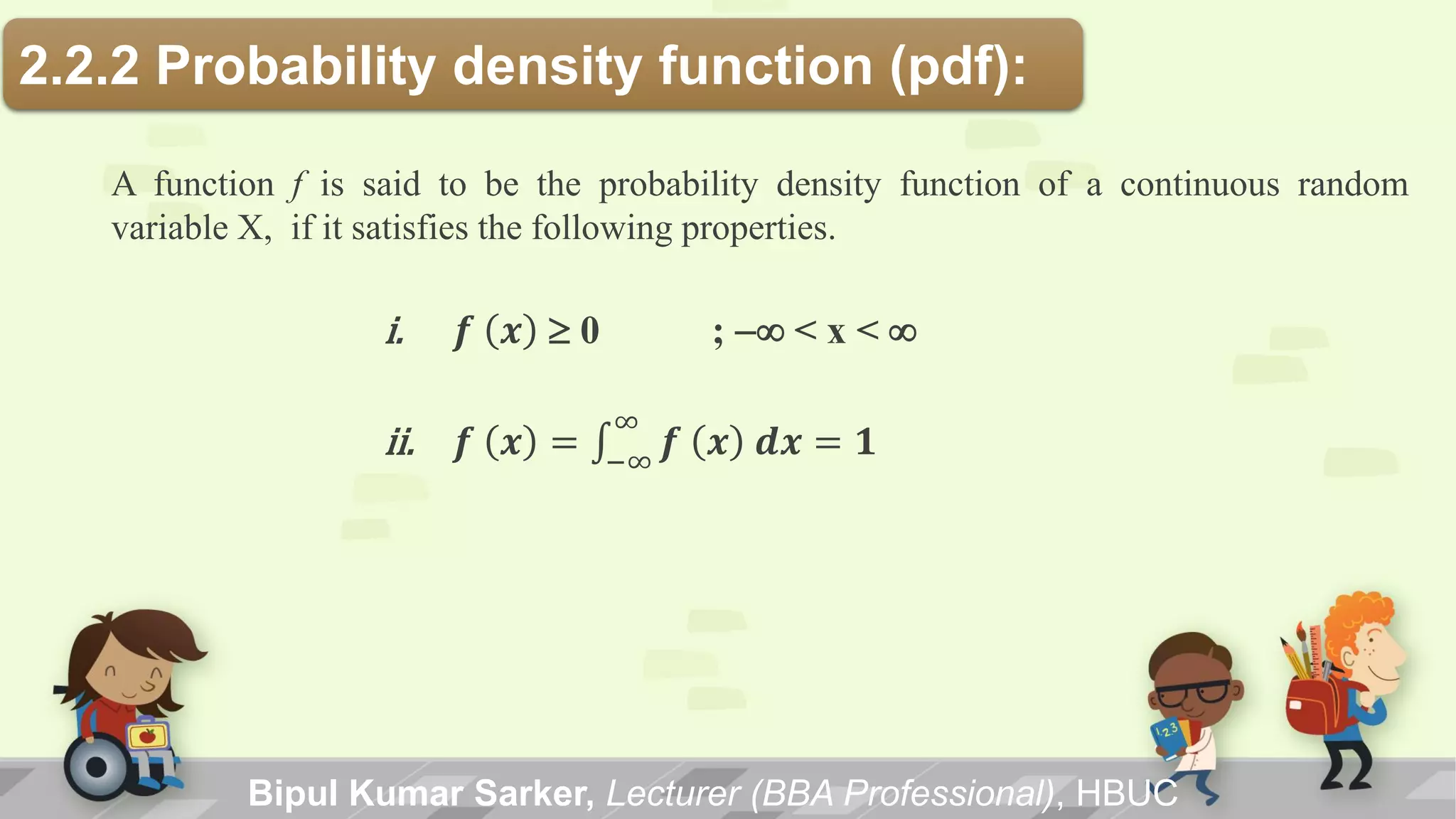
Introduction to probability density functions for continuous variables, describing its properties.
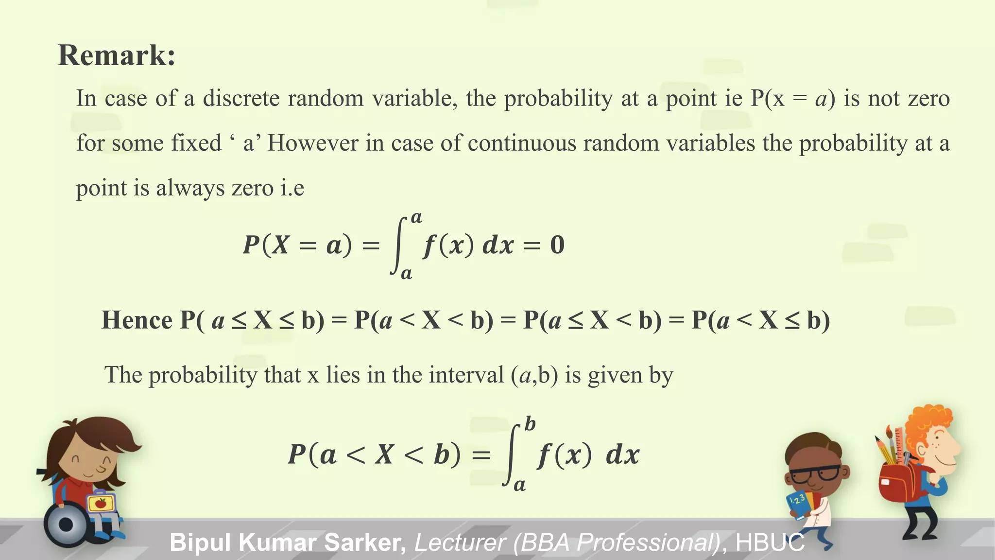
Remarks on probabilities in discrete vs continuous cases, particularly focusing on point probabilities.
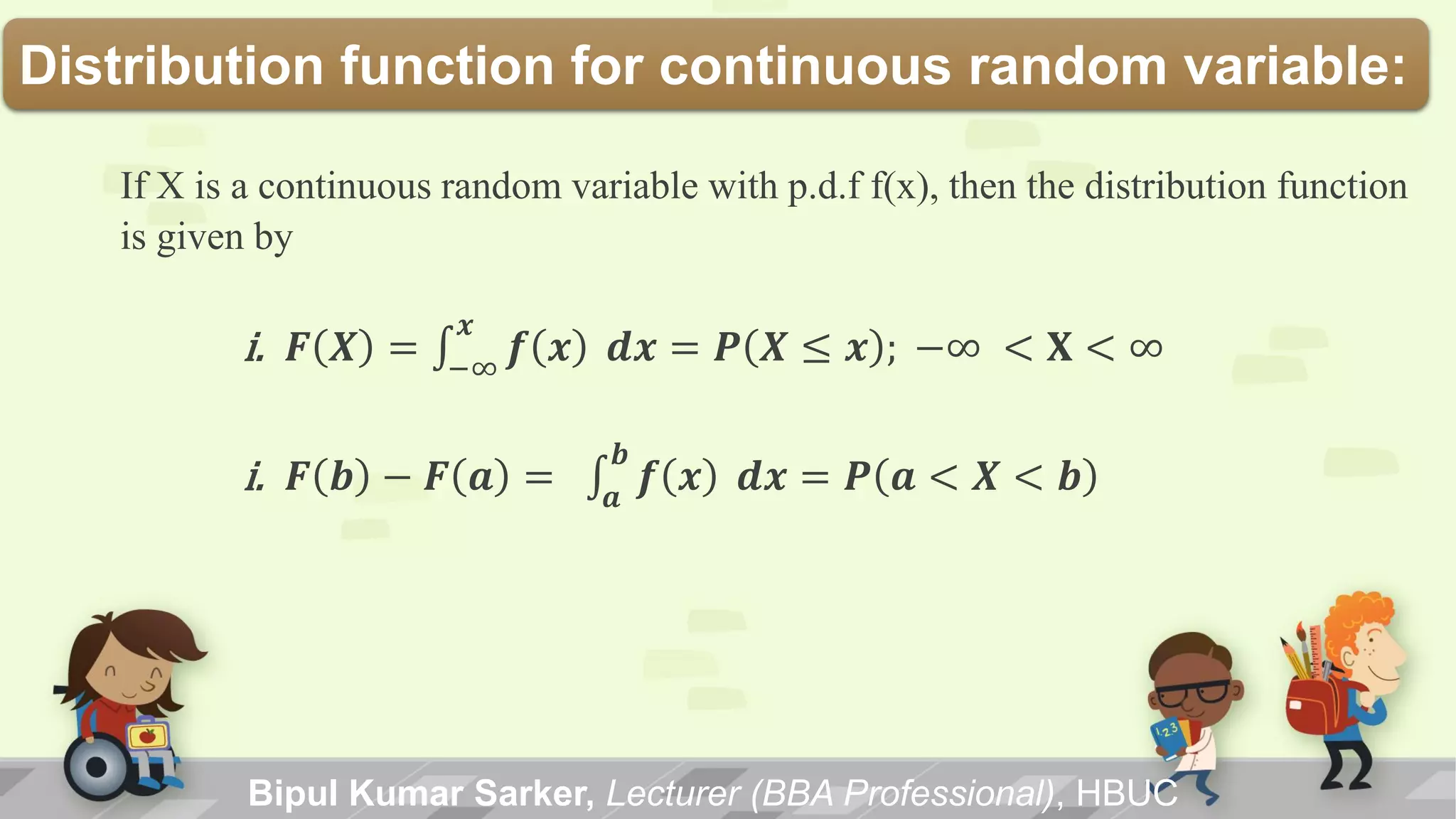
Distribution function for continuous random variables explained, detailing calculations of probabilities.
No substantial content.
No substantial content.
No substantial content.
No substantial content.
No substantial content.
No substantial content.