The document provides an outline and explanation of key concepts related to the normal distribution. It begins with an introduction to probability distributions for continuous random variables and the definition of a density curve. It then defines terms and symbols used in the normal distribution, including mean, standard deviation, and z-scores. The document explains the characteristics of the normal distribution graphically and provides examples of finding areas under the normal curve using z-tables. It concludes with examples of finding unknown z-values and calculating probabilities for specific scenarios involving the normal distribution.
TOPIC OUTLINE
TheNormal Distribution
1) Introduction
2) Definition of Terms and Statistical Symbols Used
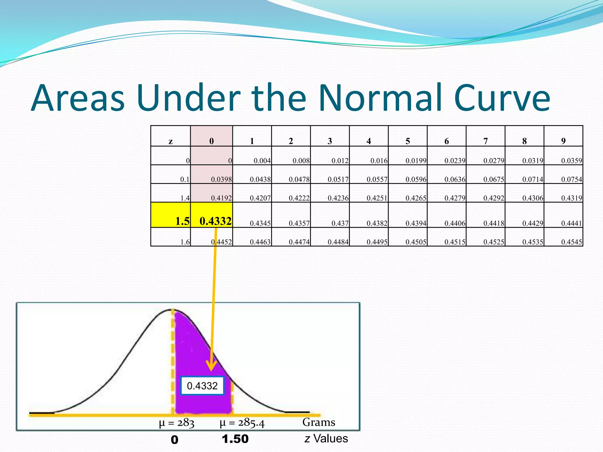
3) How To Find Areas Under the Normal Curve
4) Finding the Unknown Z represented by Zo
5) Examples
Hypothesis Testing
3.
The Normal Distribution
Introduction
Before exploring the complicated Standard
Normal Distribution, we must examine how the
concept of Probability Distribution changes when the
Random Variable is Continuous.
4.
The Normal Distribution
Introduction
A Probability Distribution will give us a Value of P(x) = P(X=x)
to each possible outcome of x. For the values to make a Probability
Distribution, we needed two things to happen:
1. P (x) = P (X = x)
2. 0 ≤ P (x) ≤ 1
For a Continuous Random Variable, a Probability Distribution
must be what is called a Density Curve. This means:
1. The Area under the Curve is 1.
2. 0 ≤ P (x) for all outcomes x.
5.
The Normal Distribution
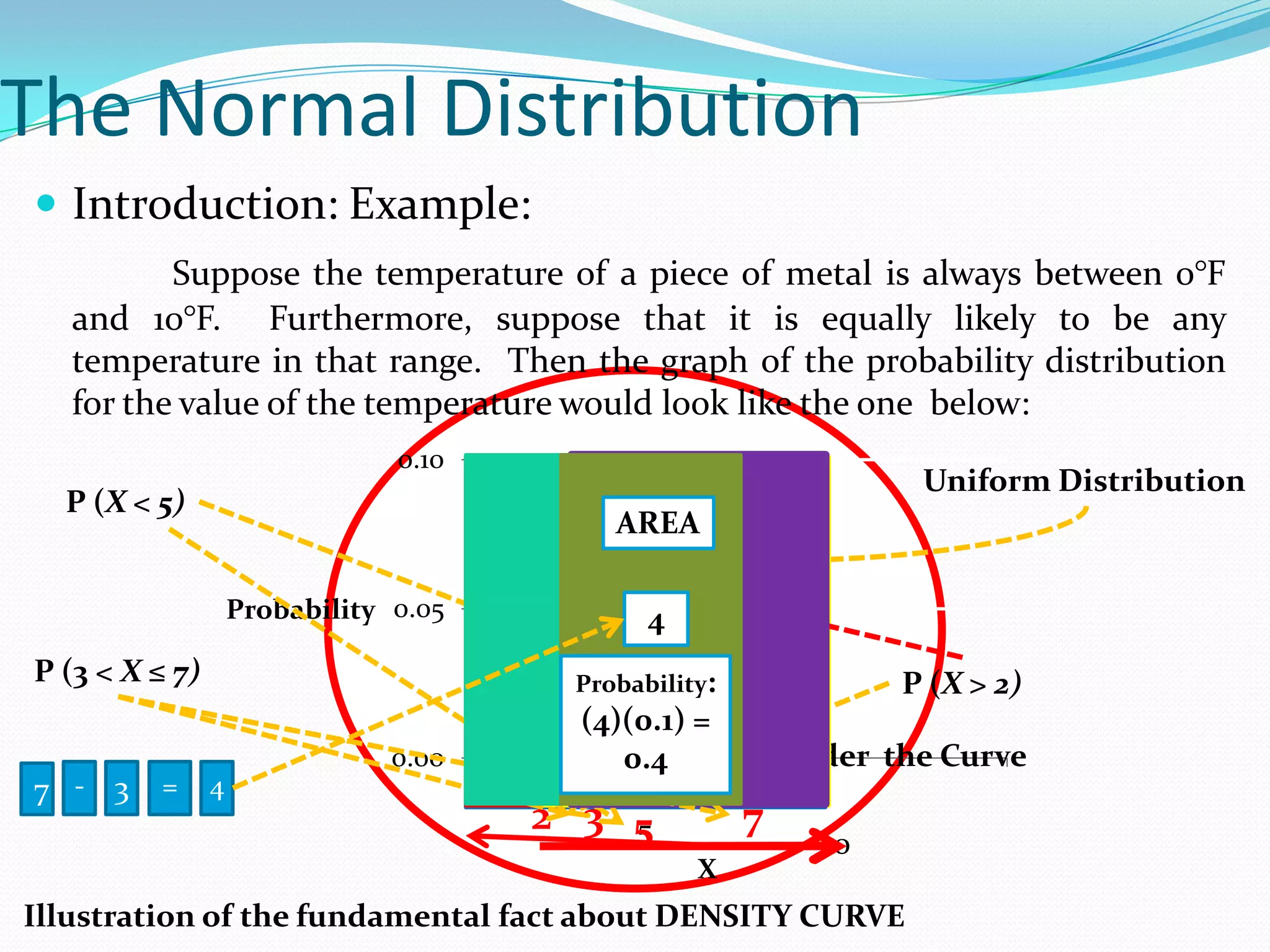
Introduction: Example:
Suppose the temperature of a piece of metal is always between 0°F
and 10°F. Furthermore, suppose that it is equally likely to be any
temperature in that range. Then the graph of the probability distribution
for the value of the temperature would look like the one below:
0.10
Uniform Distribution
P (X < 5) ValuesAREA
are spread
uniformly across
Probability 0.05 0.8
the range 0 to 10
0.5 4
P (3 < X ≤ 7) Probability:
Area: 80% P (X > 2)
(4)(0.1) =
0.00 Finding the Area Under the Curve
0.4
7 - 3 = 4
2 3 5
5 7
10
X
Illustration of the fundamental fact about DENSITY CURVE
6.
The Normal Distribution:Definition
of Terms and Symbols Used
Normal Distribution Definition:
1) A continuous variable X having the symmetrical, bell shaped distribution
is called a Normal Random Variable.
2) The normal probability distribution (Gaussian distribution) is a
continuous distribution which is regarded by many as the most significant
probability distribution in statistics particularly in the field of statistical
inference.
Symbols Used:
“z” – z-scores or the standard scores. The table that transforms every normal
distribution to a distribution with mean 0 and standard deviation 1. This
distribution is called the standard normal distribution or simply
standard distribution and the individual values are called standard
scores or the z-scores.
“µ” – the Greek letter “mu,” which is the Mean, and
“σ” – the Greek letter “sigma,” which is the Standard Deviation
7.
The Normal Distribution:Definition
of Terms and Symbols Used
Characteristics of Normal Distribution:
1) It is “Bell-Shaped” and has a single peak at the center of the
distribution,
2) The arithmetic Mean, Median and Mode are equal.
3) The total area under the curve is 1.00; half the area under the
normal curve is to the right of this center point and the other
half to the left of it,
4) It is Symmetrical about the mean,
5) It is Asymptotic: The curve gets closer and closer to the X –
axis but never actually touches it. To put it another way, the
tails of the curve extend indefinitely in both directions.
6) The location of a normal distribution is determined by the
Mean, µ, the Dispersion or spread of the distribution is
determined by the Standard Deviation, σ.
8.
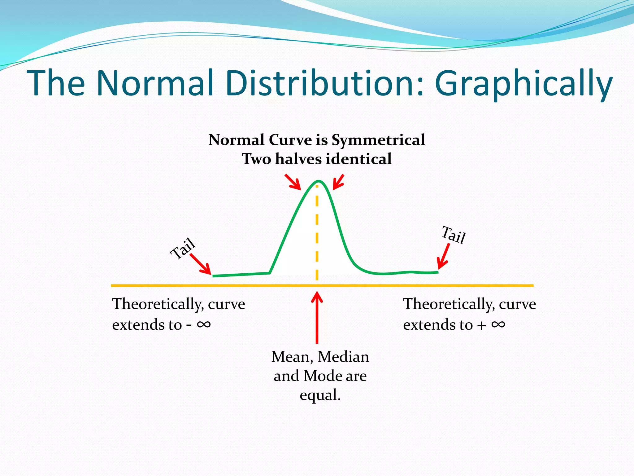
The Normal Distribution:Graphically
Normal Curve is Symmetrical
Two halves identical
Theoretically, curve Theoretically, curve
extends to - ∞ extends to + ∞
Mean, Median
and Mode are
equal.
9.
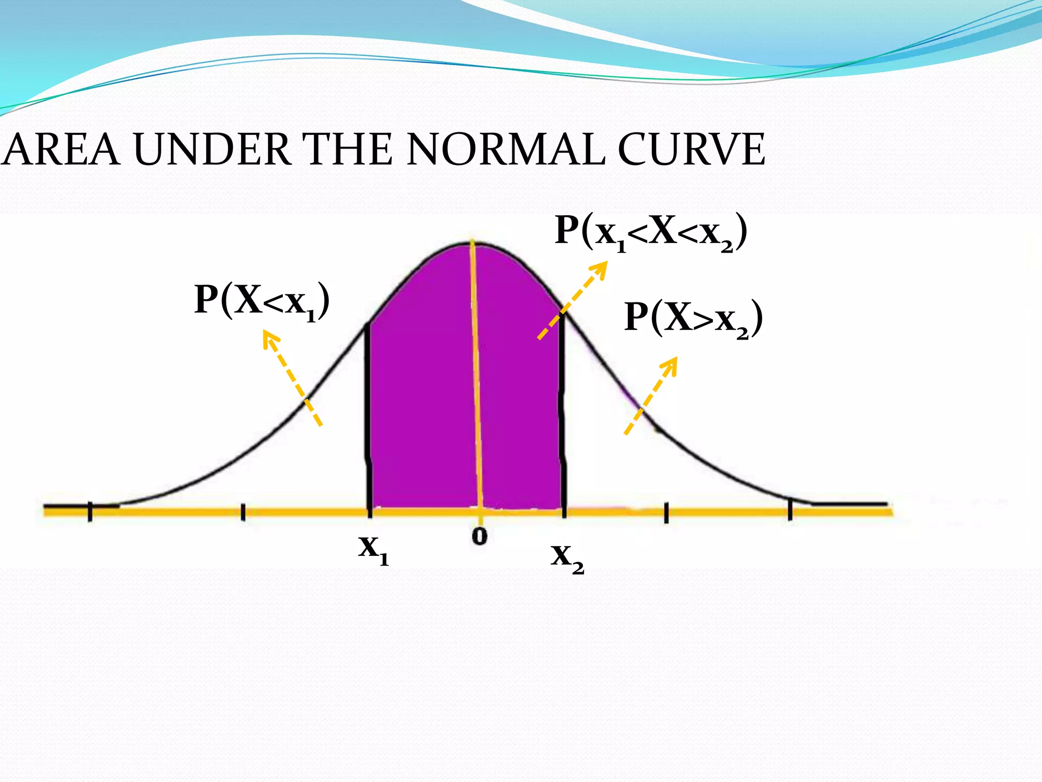
AREA UNDER THENORMAL CURVE
P(x1<X<x2)
P(X<x1) P(X>x2)
x1 x2
10.
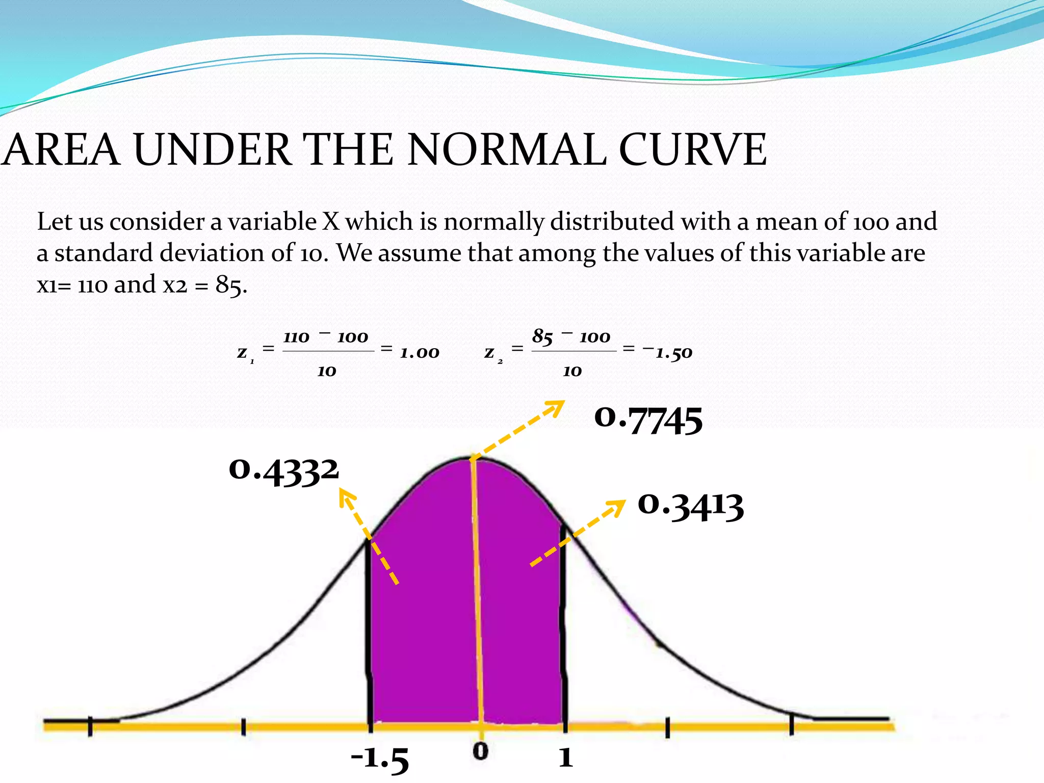
AREA UNDER THENORMAL CURVE
Let us consider a variable X which is normally distributed with a mean of 100 and
a standard deviation of 10. We assume that among the values of this variable are
x1= 110 and x2 = 85.
110 100 85 100
z1 1 . 00 z2 1 . 50
10 10
0.7745
0.4332
0.3413
-1.5 1
11.
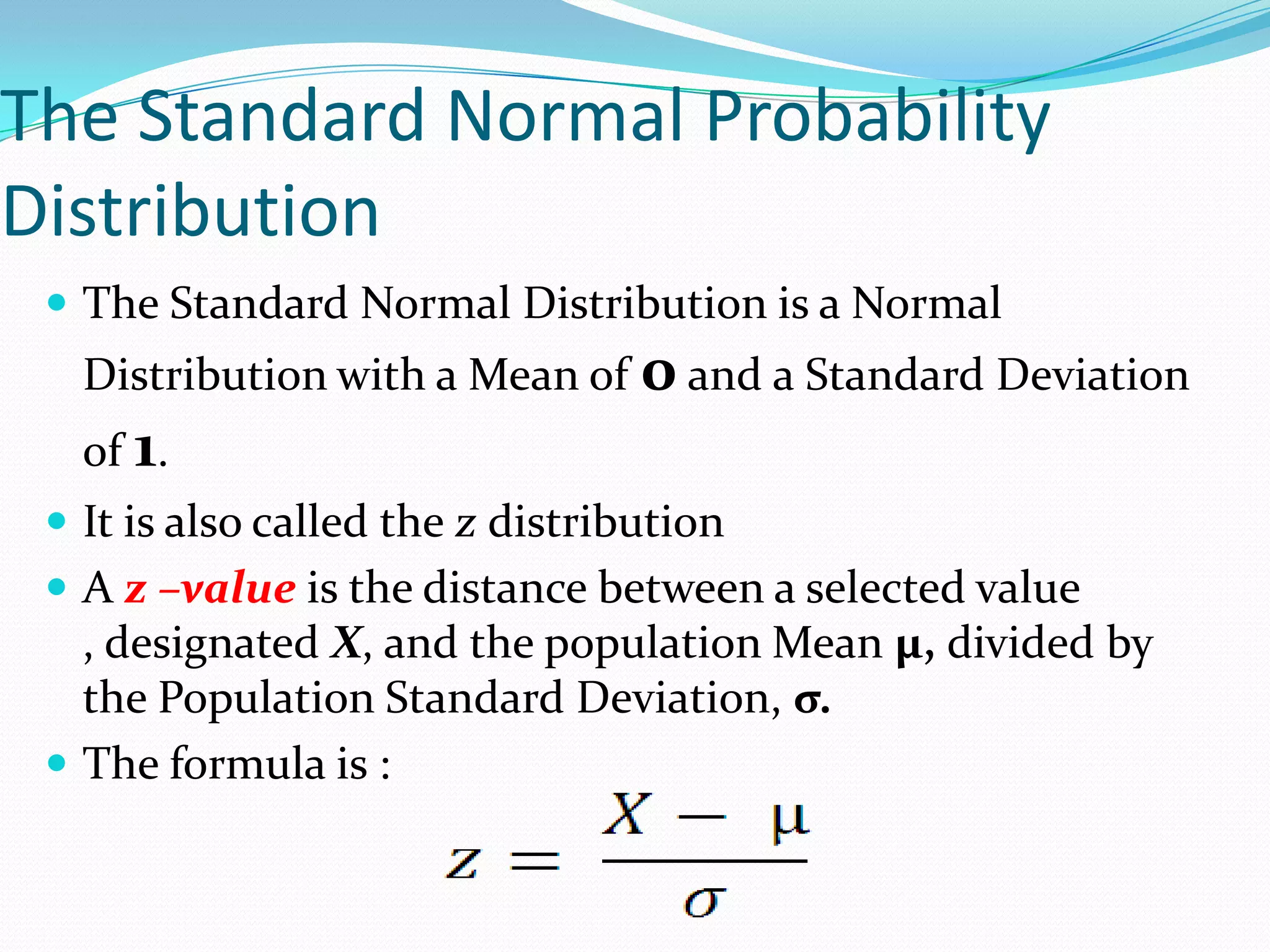
The Standard NormalProbability
Distribution
The Standard Normal Distribution is a Normal
Distribution with a Mean of 0 and a Standard Deviation
of 1.
It is also called the z distribution
A z –value is the distance between a selected value
, designated X, and the population Mean µ, divided by
the Population Standard Deviation, σ.
The formula is :
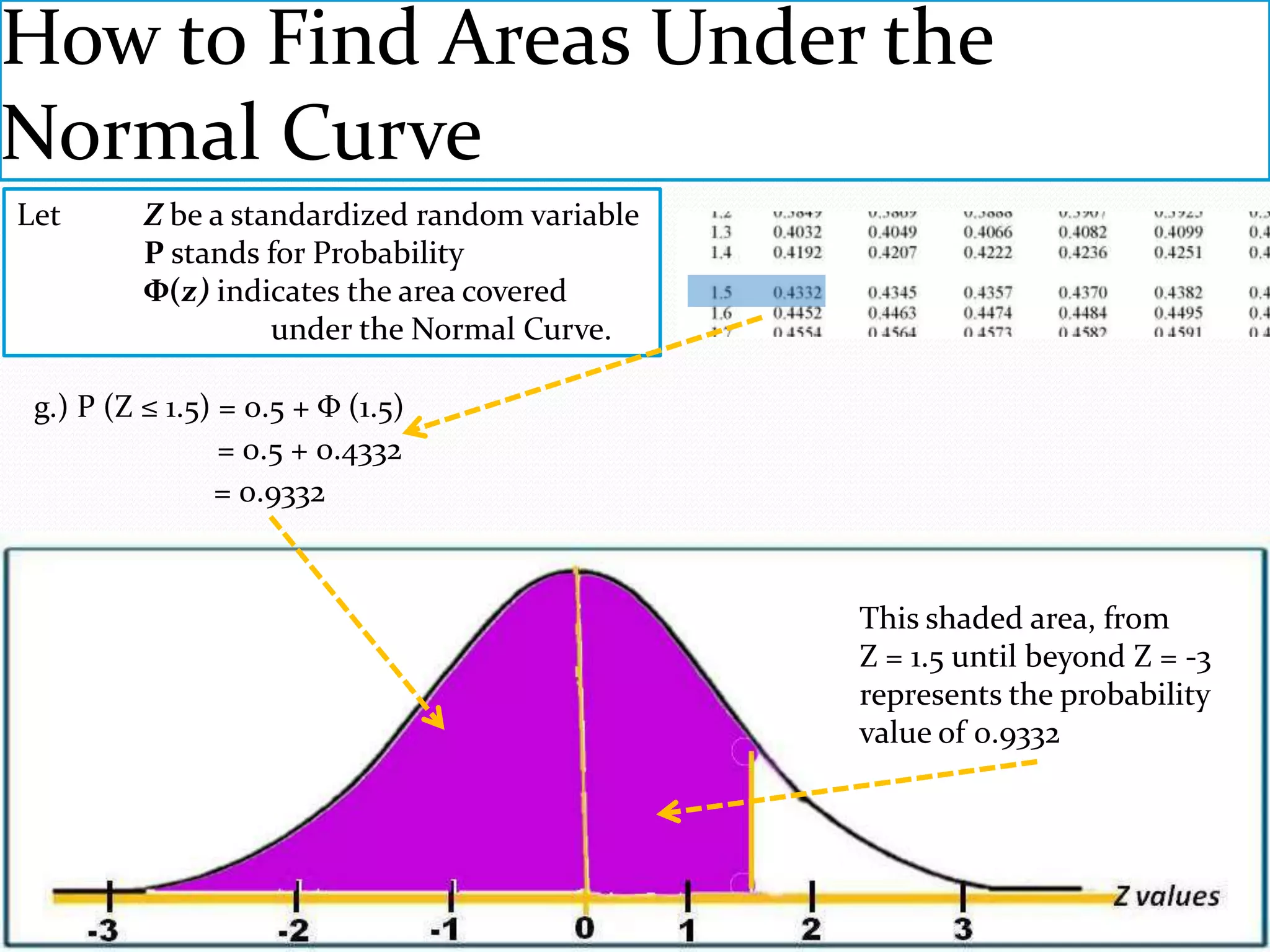
How to FindAreas Under the
Normal Curve
Let Z be a standardized random variable
P stands for Probability
Φ(z) indicates the area covered
under the Normal Curve.
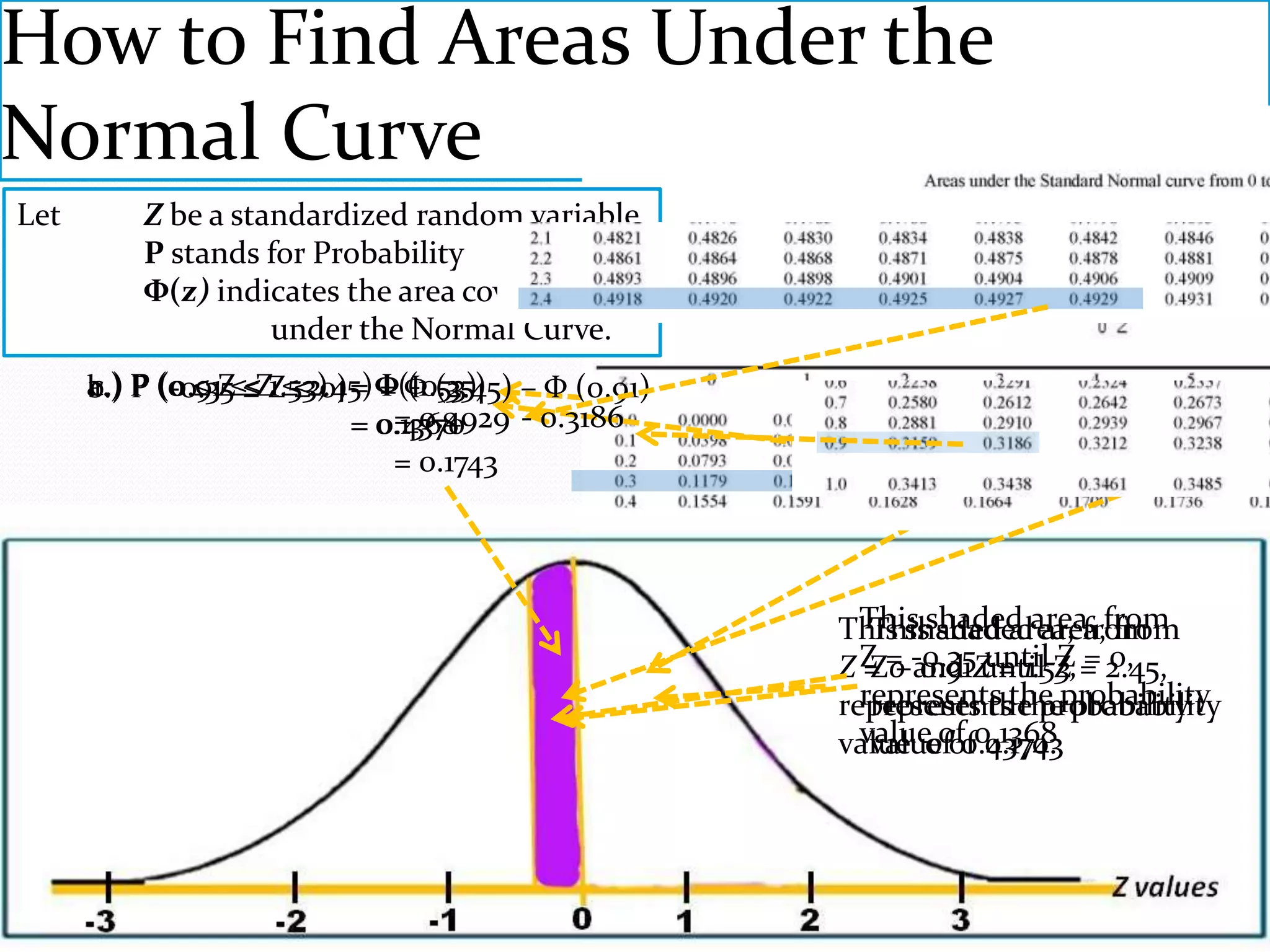
a.) P (0 ≤ Z≤≤ZZ≤≤2.45) Φ(-0.35) – Φ (0.91)
b.) (-0.35 1.53) = Φ Φ (2.45)
c.) (0.91 0) = (1.53)
= 0.4929 - 0.3186
= 0.1368
0.4370
= 0.1743
This shaded area, from
This shaded area, from
This shaded area, from
Z Z = -0.35Z = 1.53, = 2.45,
= 0 and until Z = 0,
Z – 0.91 until Z
represents the probability
represents the probability
represents the probability
value ofof0.1368
value of0.4370.
value 0.1743
14.
How to FindAreas Under the
Normal Curve
Let Z be a standardized random variable
P stands for Probability
Φ(z) indicates the area covered
under the Normal Curve.
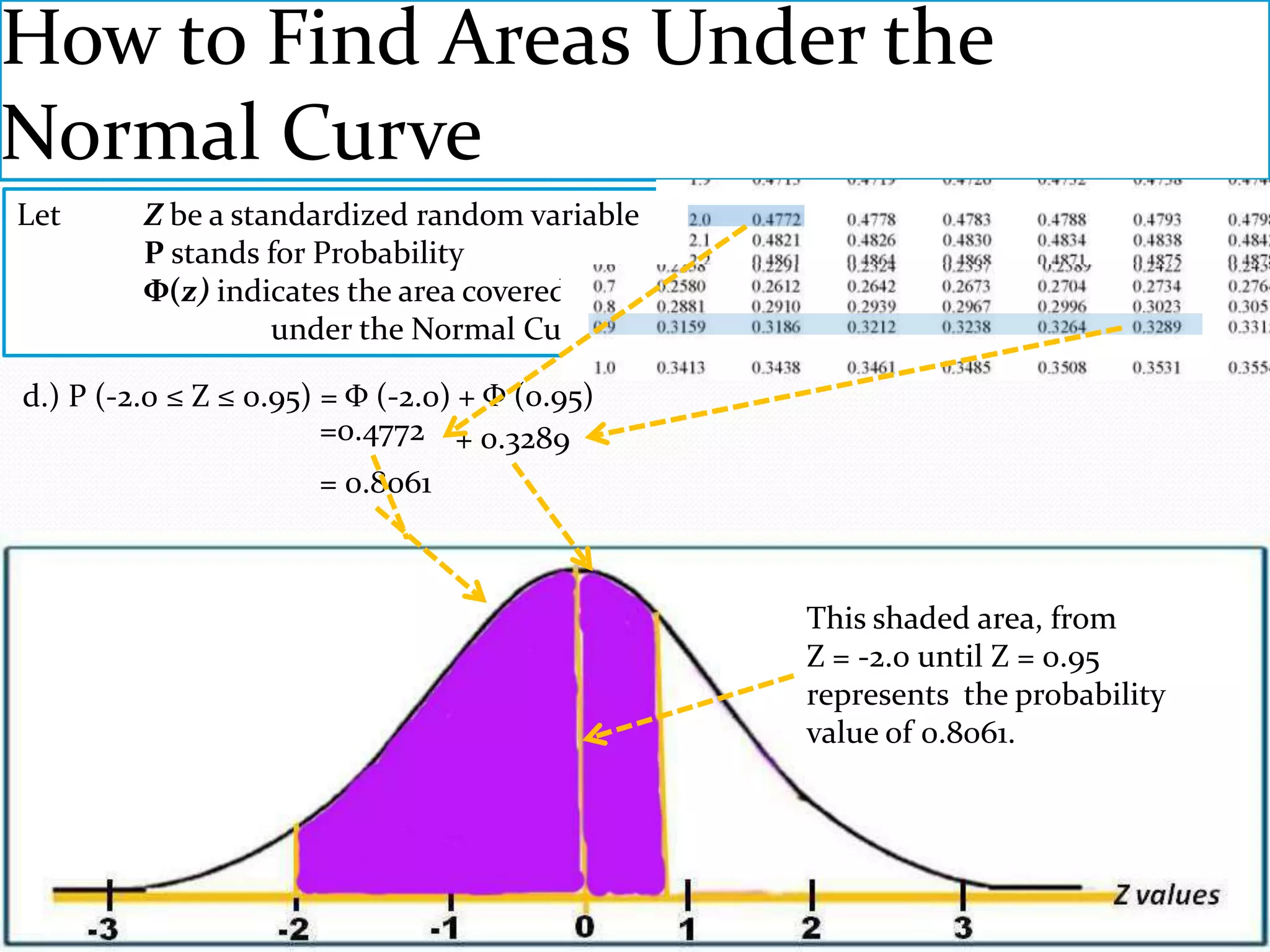
d.) P (-2.0 ≤ Z ≤ 0.95) = Φ (-2.0) + Φ (0.95)
=0.4772 + 0.3289
= 0.8061
This shaded area, from
Z = -2.0 until Z = 0.95
represents the probability
value of 0.8061.
15.
How to FindAreas Under the
Normal Curve
Let Z be a standardized random variable
P stands for Probability
Φ(z) indicates the area covered
under the Normal Curve.
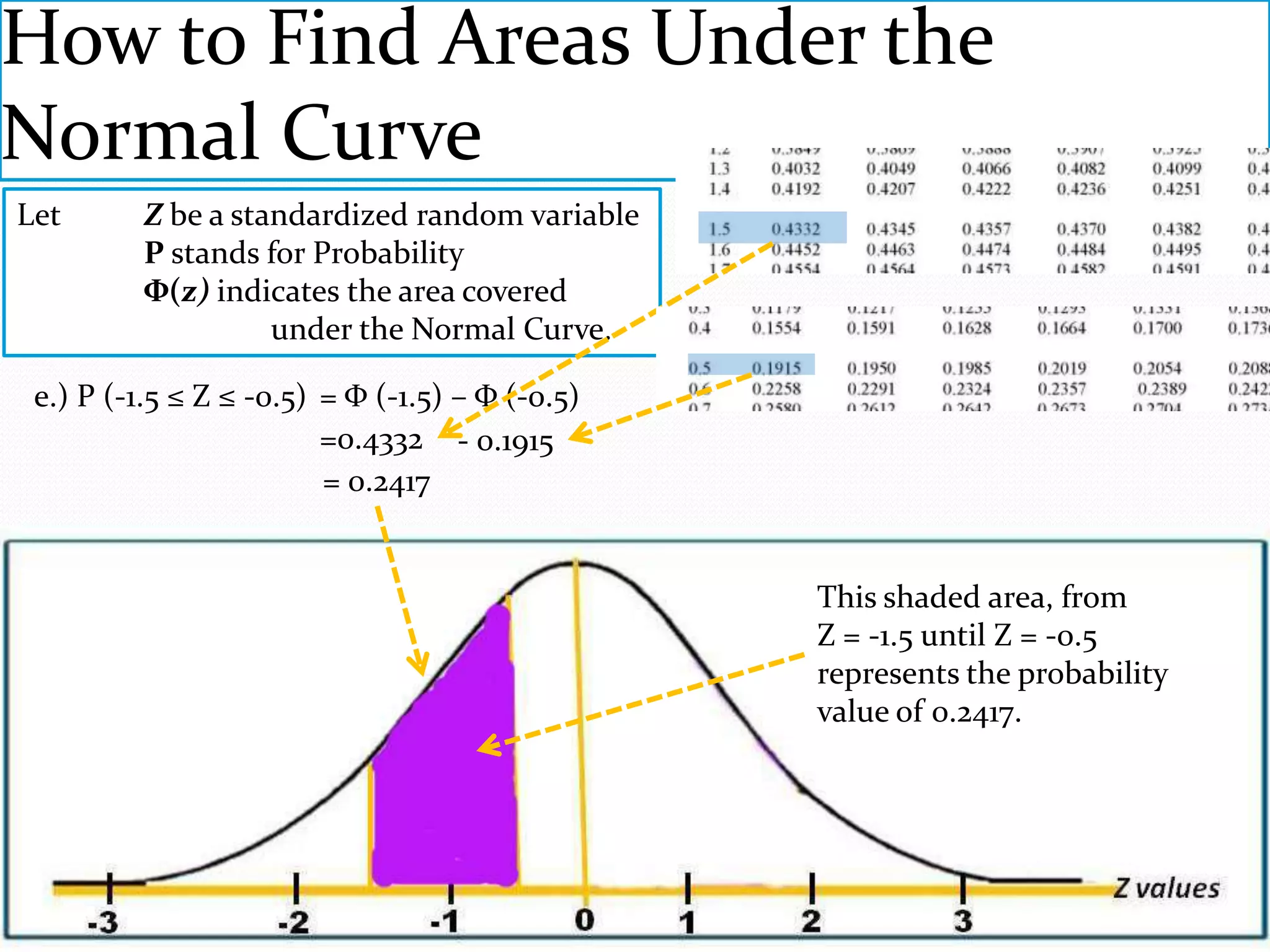
e.) P (-1.5 ≤ Z ≤ -0.5) = Φ (-1.5) – Φ (-0.5)
=0.4332 - 0.1915
= 0.2417
This shaded area, from
Z = -1.5 until Z = -0.5
represents the probability
value of 0.2417.
16.
How to FindAreas Under the
Normal Curve
Let Z be a standardized random variable
P stands for Probability
Φ(z) indicates the area covered
under the Normal Curve.
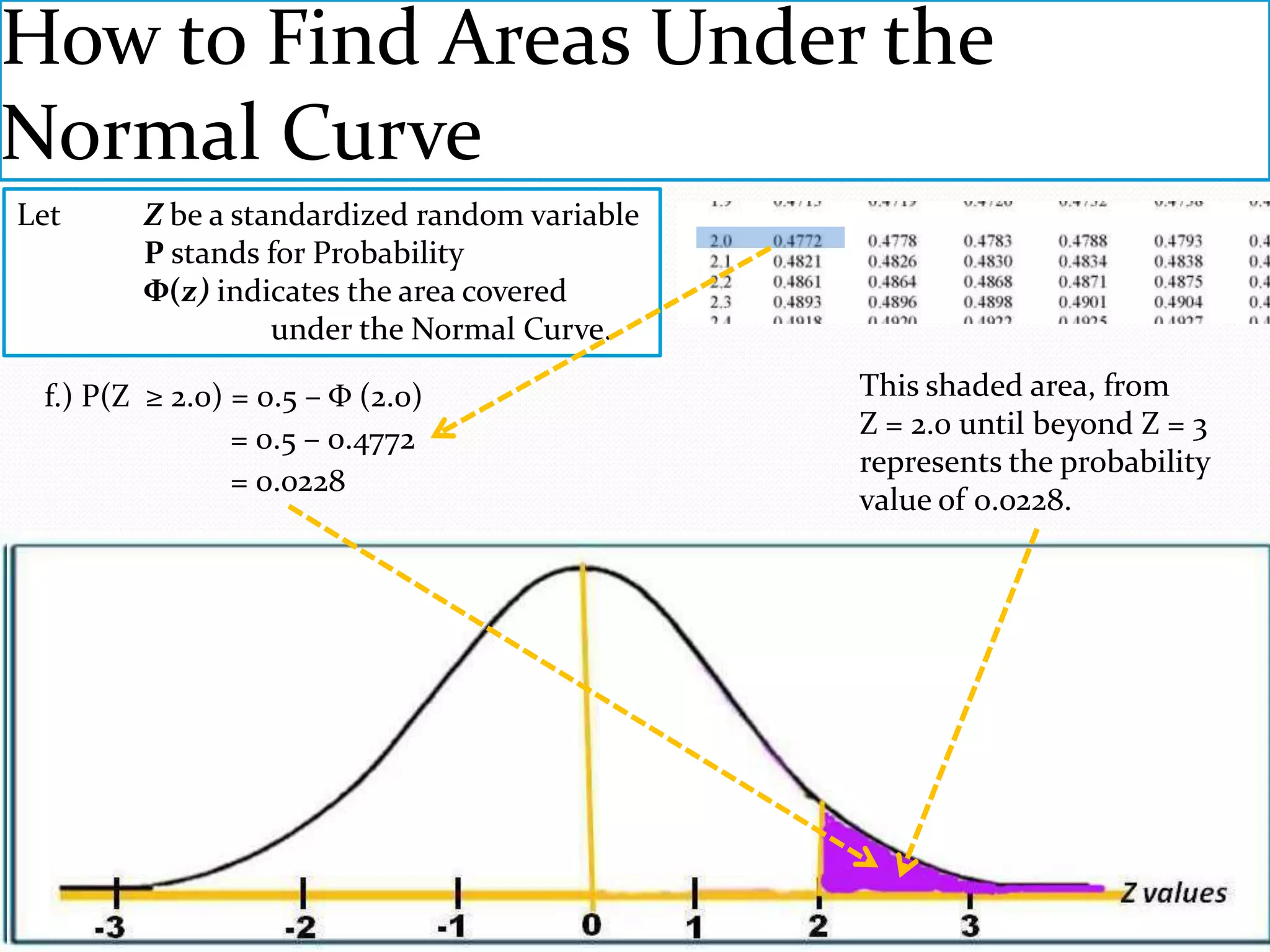
f.) P(Z ≥ 2.0) = 0.5 – Φ (2.0) This shaded area, from
= 0.5 – 0.4772 Z = 2.0 until beyond Z = 3
represents the probability
= 0.0228
value of 0.0228.
17.
How to FindAreas Under the
Normal Curve
Let Z be a standardized random variable
P stands for Probability
Φ(z) indicates the area covered
under the Normal Curve.
g.) P (Z ≤ 1.5) = 0.5 + Φ (1.5)
= 0.5 + 0.4332
= 0.9332
This shaded area, from
Z = 1.5 until beyond Z = -3
represents the probability
value of 0.9332
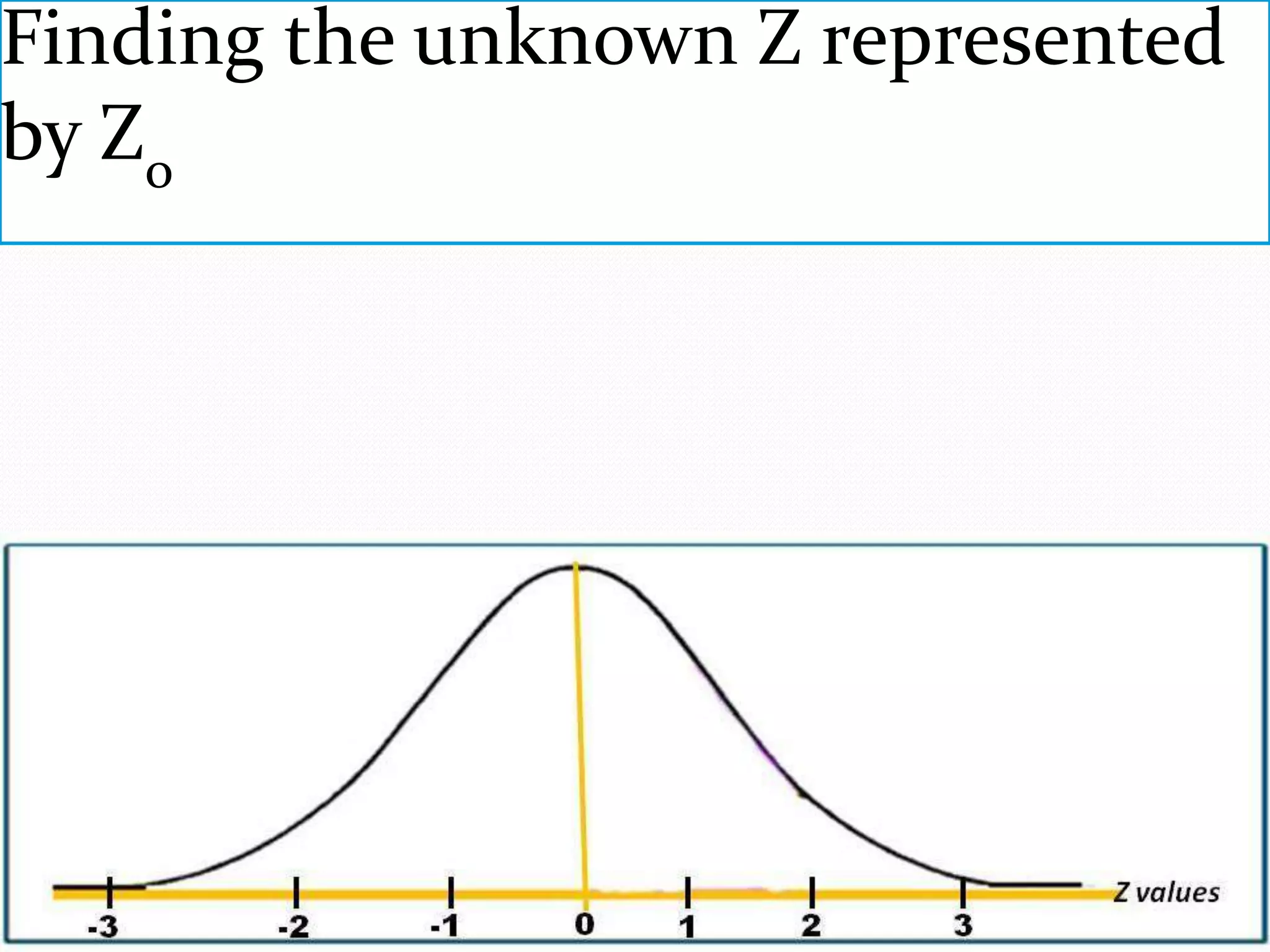
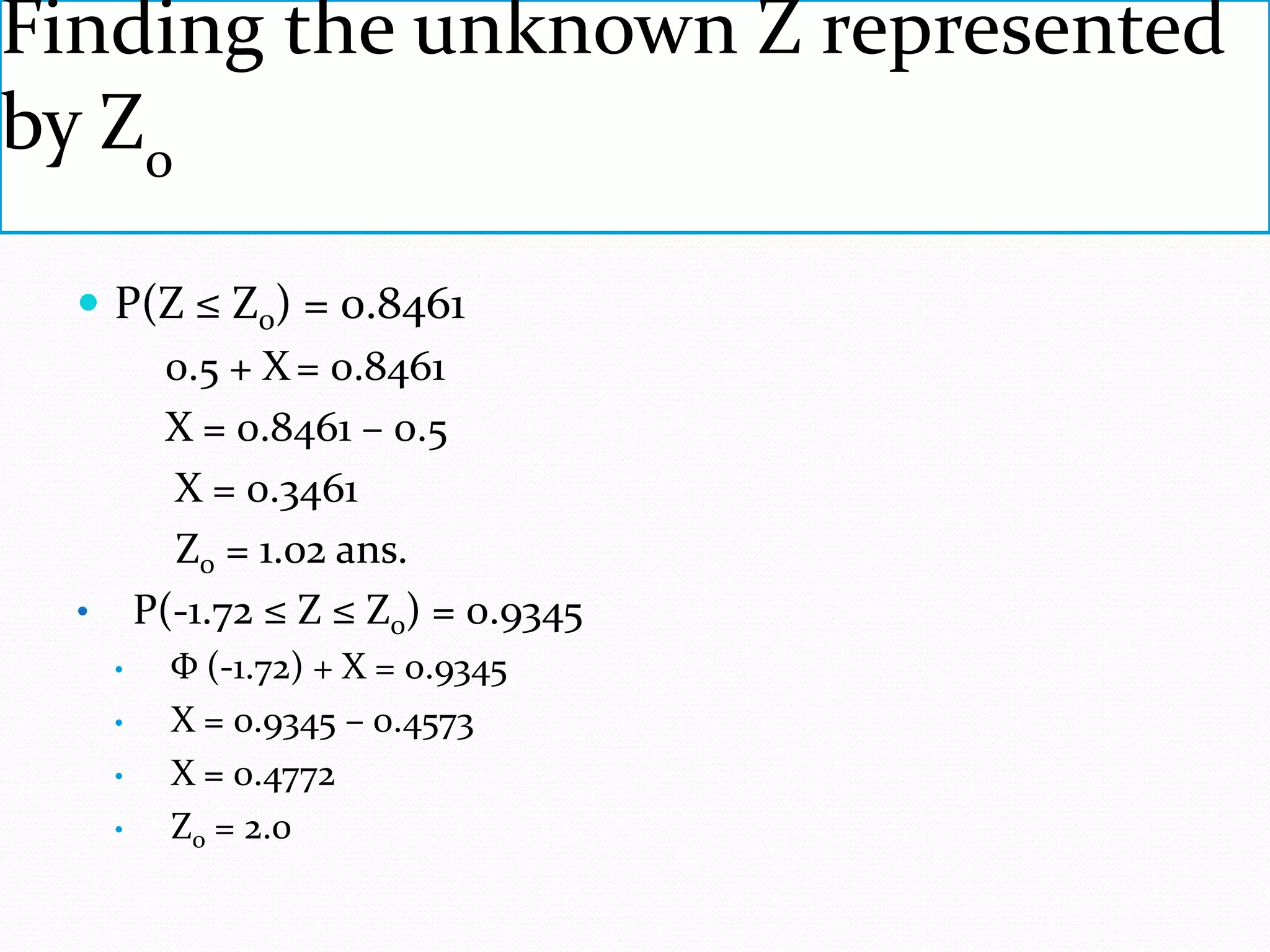
Finding the unknownZ represented
by Zo
P(Z ≤ Z0) = 0.8461
0.5 + X = 0.8461
X = 0.8461 – 0.5
X = 0.3461
Z0 = 1.02 ans.
• P(-1.72 ≤ Z ≤ Z0) = 0.9345
• Φ (-1.72) + X = 0.9345
• X = 0.9345 – 0.4573
• X = 0.4772
• Z0 = 2.0
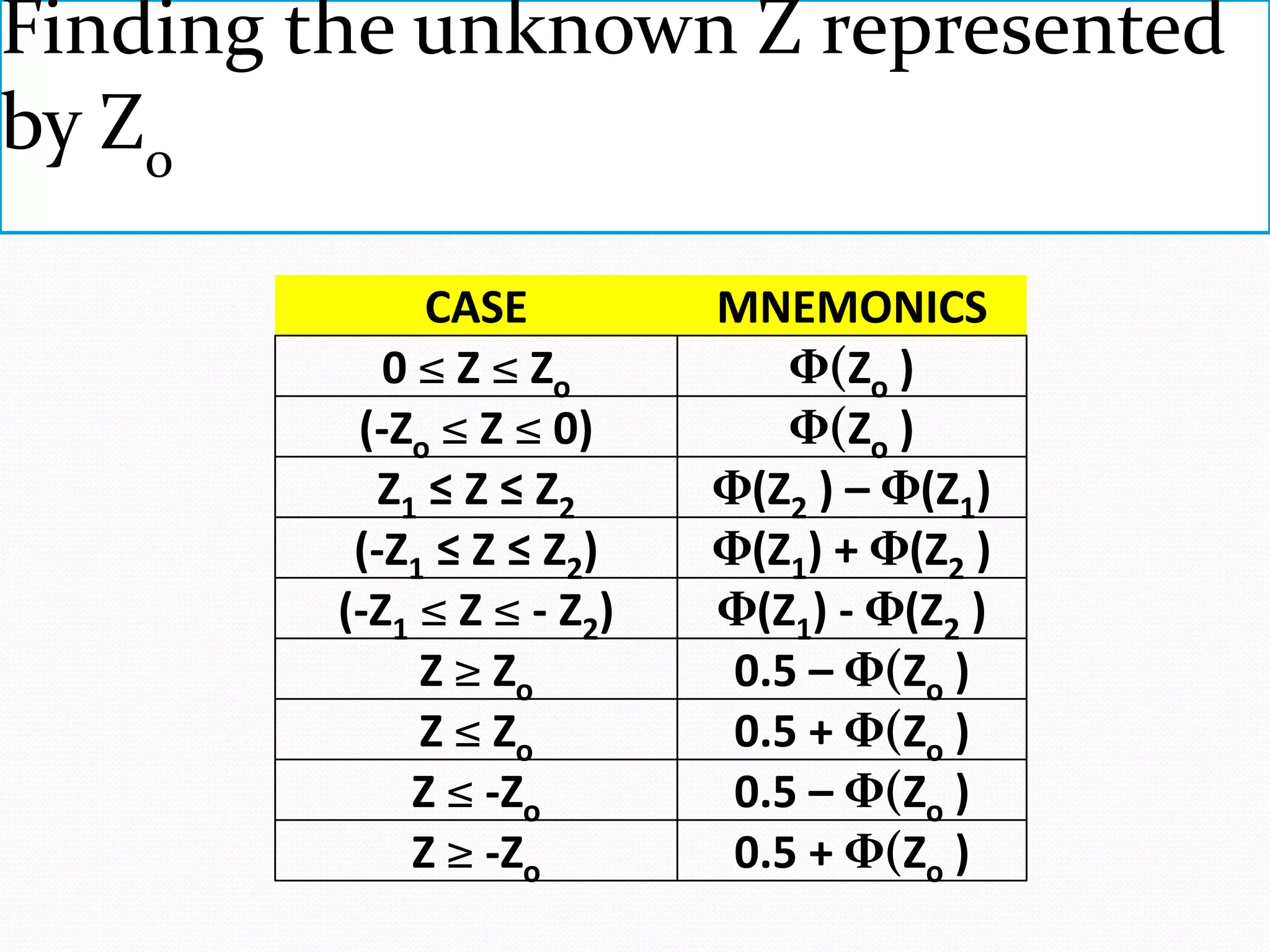
20.
Finding the unknownZ represented
by Zo
CASE MNEMONICS
0 ≤ Z ≤ Zo Φ(Zo )
(-Zo ≤ Z ≤ 0) Φ(Zo )
Z1 ≤ Z ≤ Z2 Φ(Z2 ) – Φ(Z1)
(-Z1 ≤ Z ≤ Z2) Φ(Z1) + Φ(Z2 )
(-Z1 ≤ Z ≤ - Z2) Φ(Z1) - Φ(Z2 )
Z ≥ Zo 0.5 – Φ(Zo )
Z ≤ Zo 0.5 + Φ(Zo )
Z ≤ -Zo 0.5 – Φ(Zo )
Z ≥ -Zo 0.5 + Φ(Zo )
21.
The event Xhas a normal distribution with mean µ = 10 and
Variance = 9. Find the probability that it will fall:
a.) between 10 and 11
b.) between 12 and 19
c.) above 13
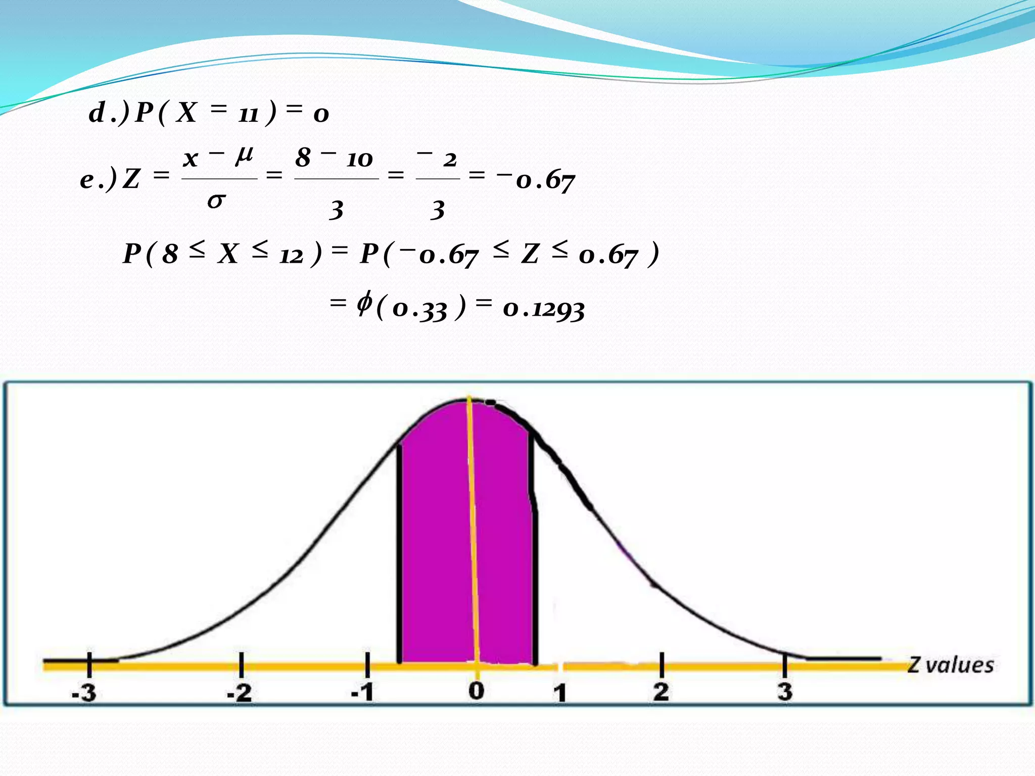
d.) at x = 11
e.) between 8 amd 12
22.
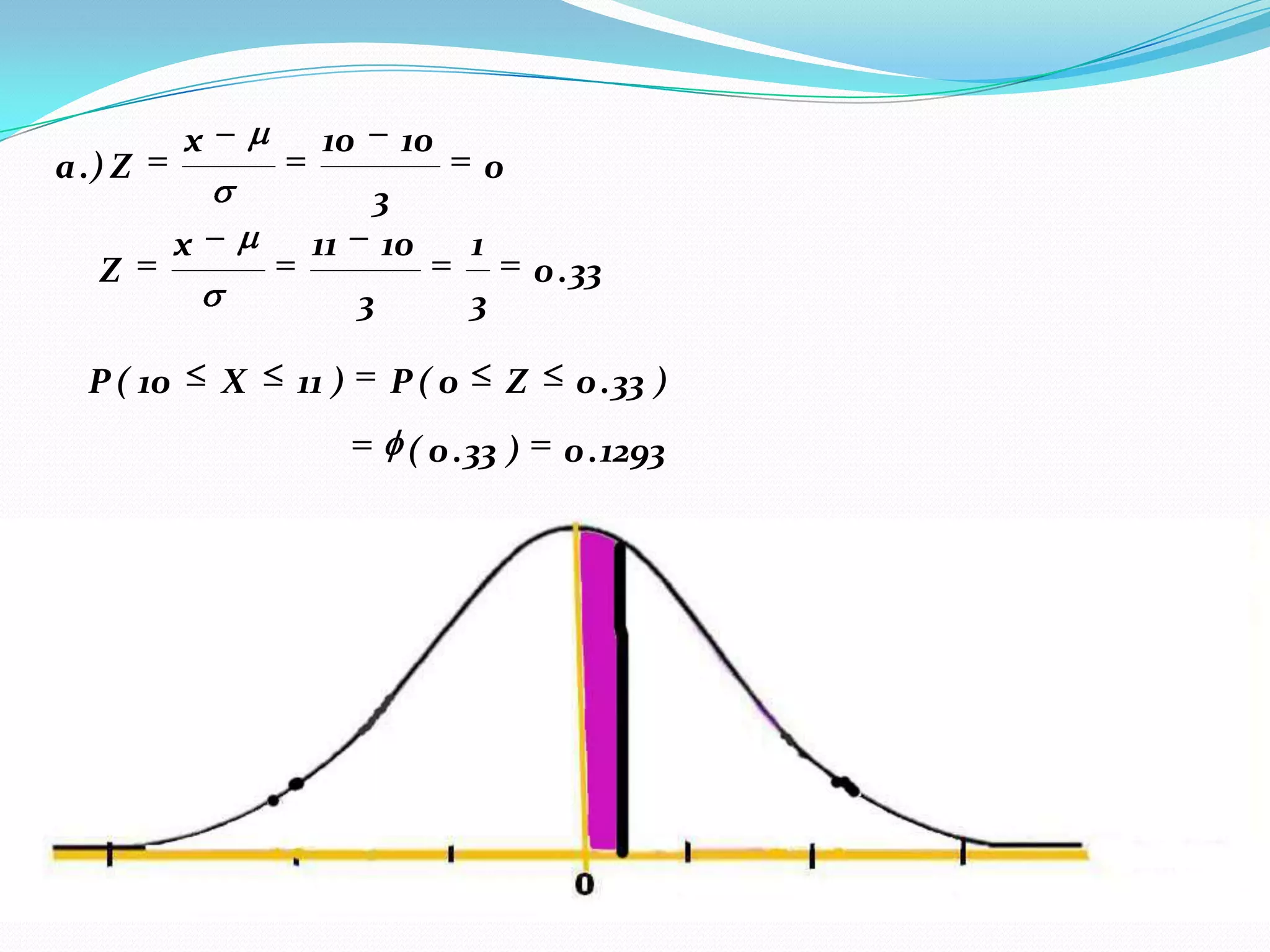
x 10 10
a .) Z 0
3
x 11 10 1
Z 0 . 33
3 3
P ( 10 X 11 ) P(0 Z 0 . 33 )
( 0 . 33 ) 0 . 1293
23.
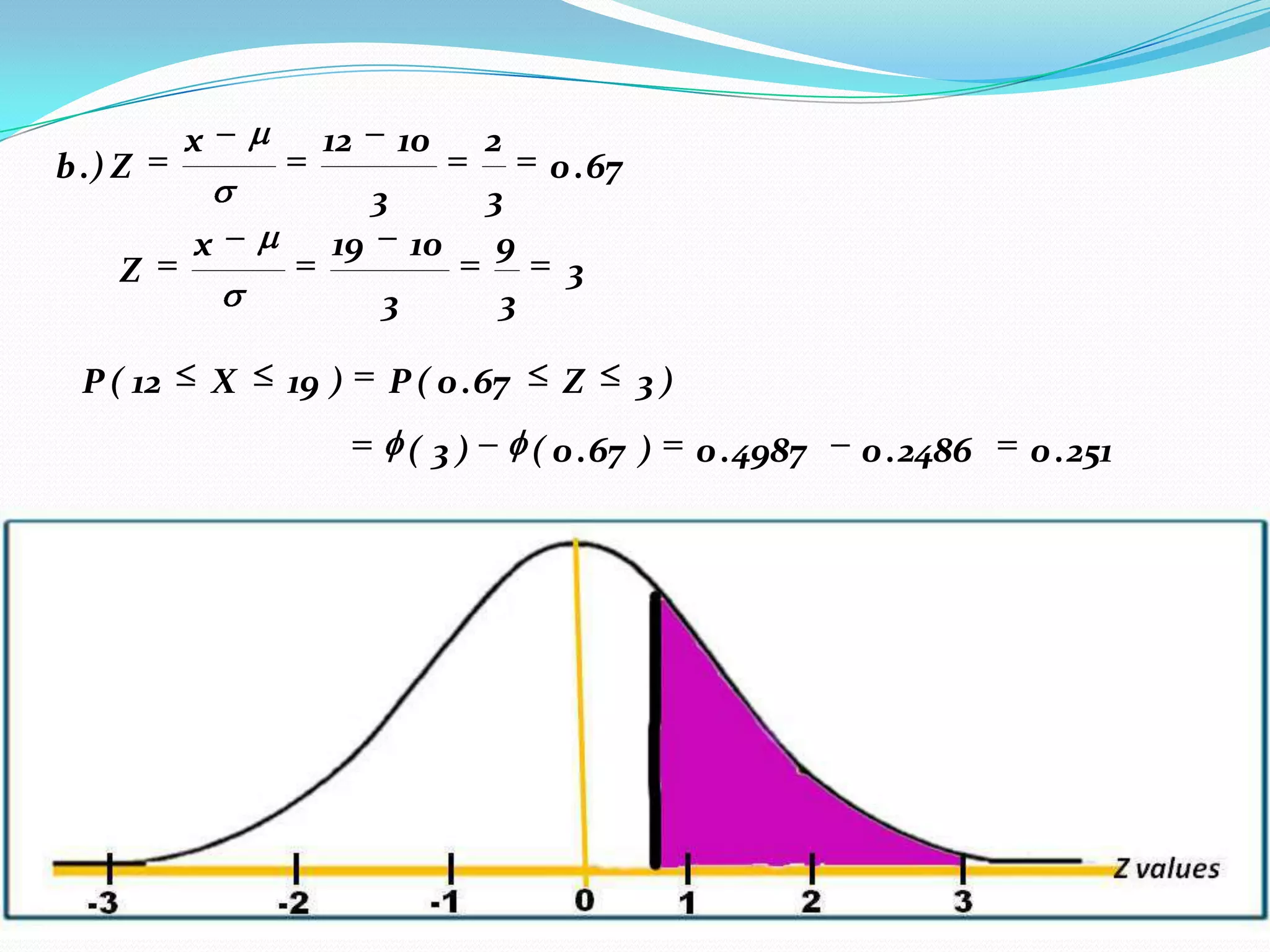
x 12 10 2
b .) Z 0 . 67
3 3
x 19 10 9
Z 3
3 3
P ( 12 X 19 ) P ( 0 . 67 Z 3)
( 3) ( 0 . 67 ) 0 . 4987 0 . 2486 0 . 251
24.
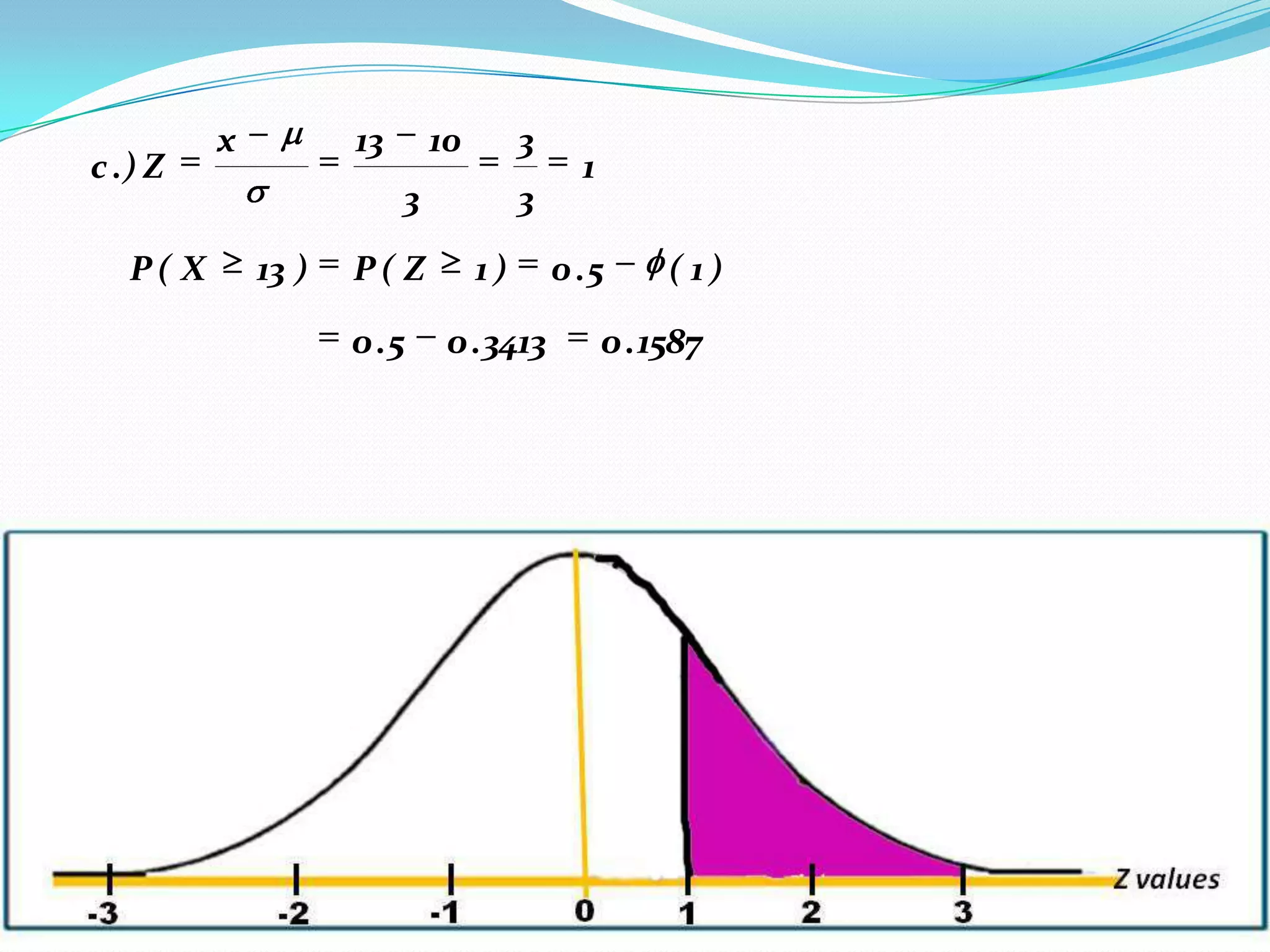
x 13 10 3
c .) Z 1
3 3
P( X 13 ) P( Z 1) 0 .5 ( 1)
0 .5 0 . 3413 0 . 1587
25.
d .) P( X 11 ) 0
x 8 10 2
e .) Z 0 . 67
3 3
P( 8 X 12 ) P ( 0 . 67 Z 0 . 67 )
( 0 . 33 ) 0 . 1293
26.
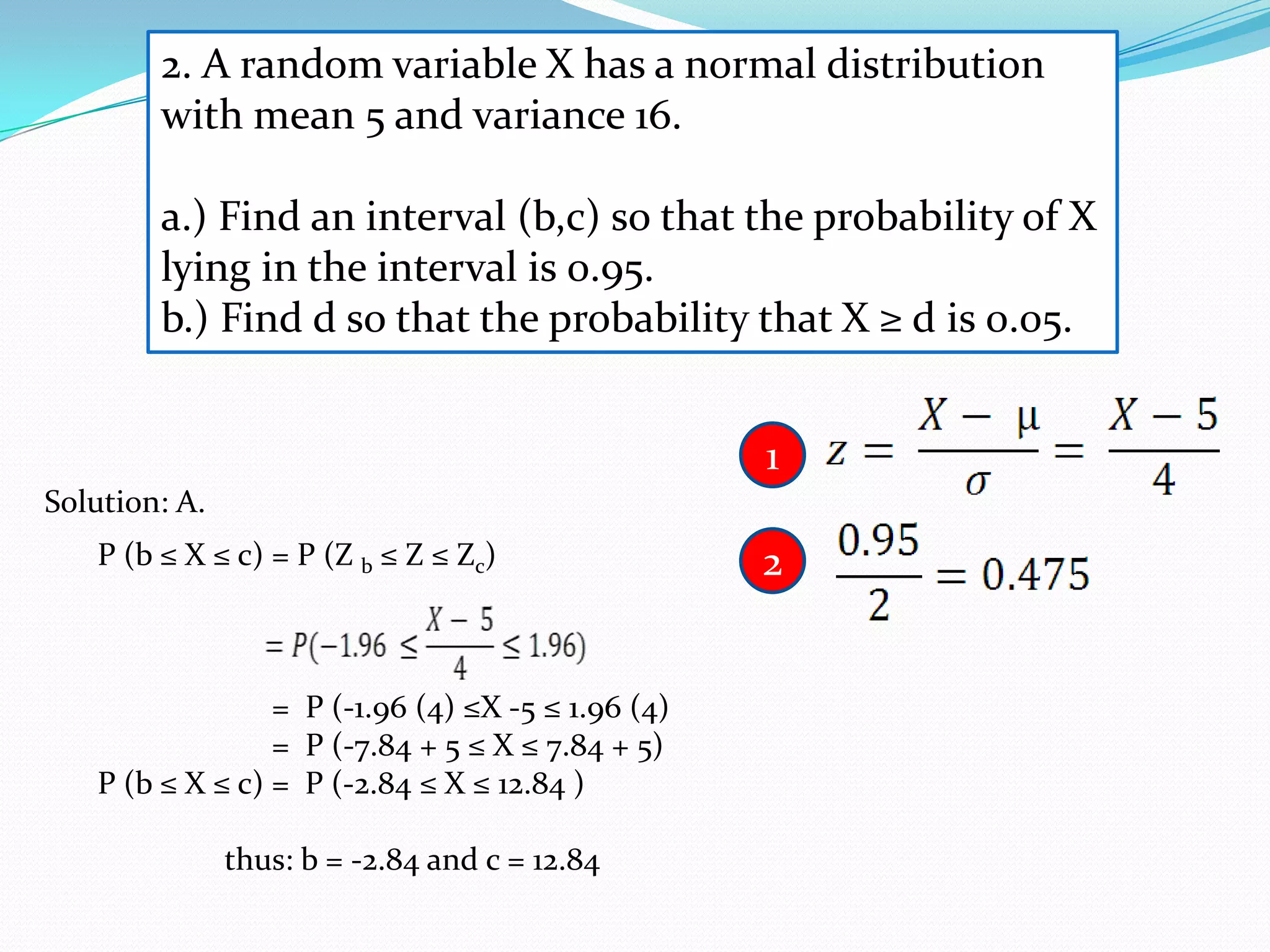
2. A randomvariable X has a normal distribution
with mean 5 and variance 16.
a.) Find an interval (b,c) so that the probability of X
lying in the interval is 0.95.
b.) Find d so that the probability that X ≥ d is 0.05.
1
Solution: A.
P (b ≤ X ≤ c) = P (Z b ≤ Z ≤ Zc) 2
= P (-1.96 (4) ≤X -5 ≤ 1.96 (4)
= P (-7.84 + 5 ≤ X ≤ 7.84 + 5)
P (b ≤ X ≤ c) = P (-2.84 ≤ X ≤ 12.84 )
thus: b = -2.84 and c = 12.84
27.
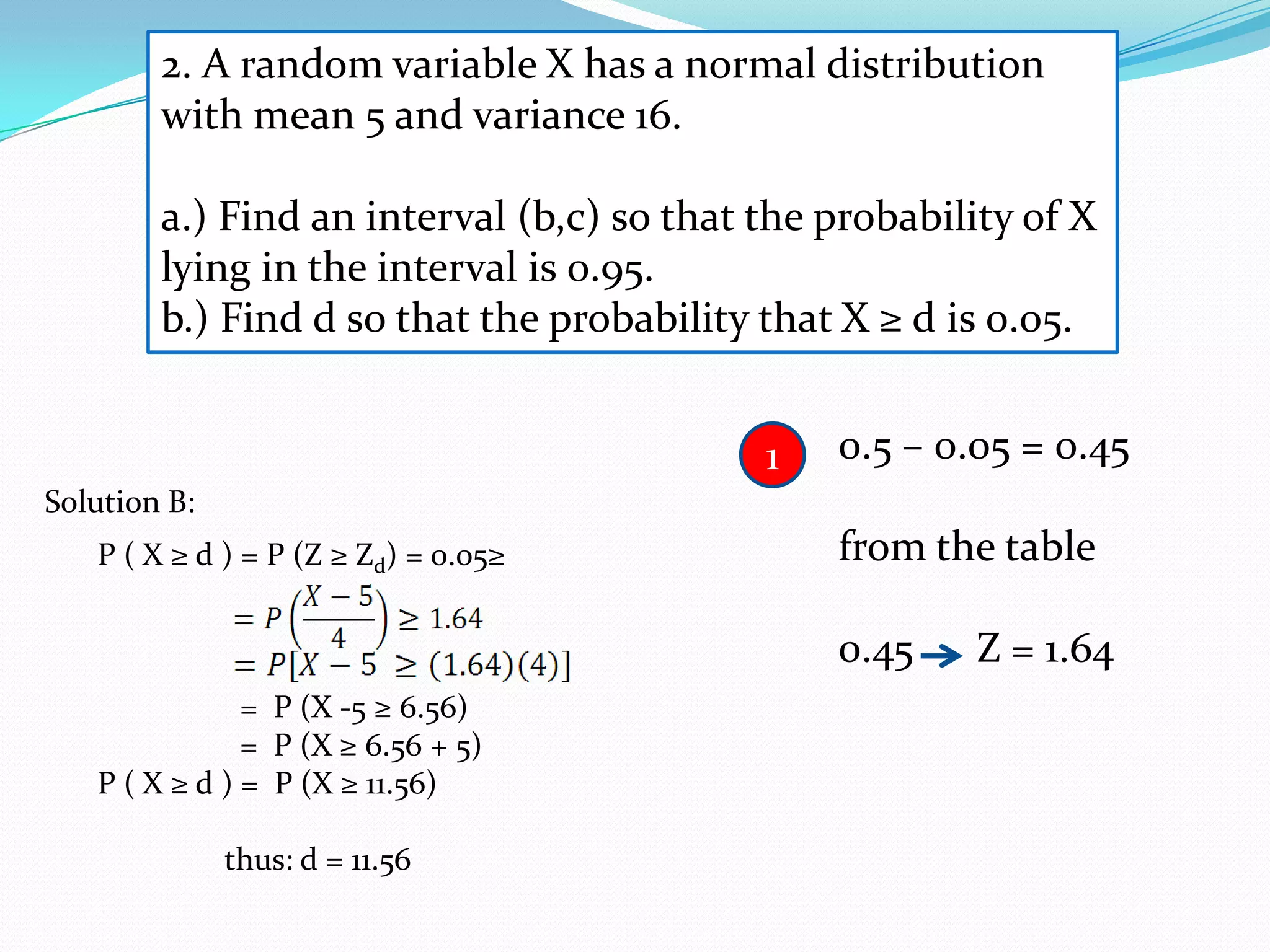
2. A randomvariable X has a normal distribution
with mean 5 and variance 16.
a.) Find an interval (b,c) so that the probability of X
lying in the interval is 0.95.
b.) Find d so that the probability that X ≥ d is 0.05.
1 0.5 – 0.05 = 0.45
Solution B:
P ( X ≥ d ) = P (Z ≥ Zd) = 0.05≥ from the table
0.45 Z = 1.64
= P (X -5 ≥ 6.56)
= P (X ≥ 6.56 + 5)
P ( X ≥ d ) = P (X ≥ 11.56)
thus: d = 11.56
28.
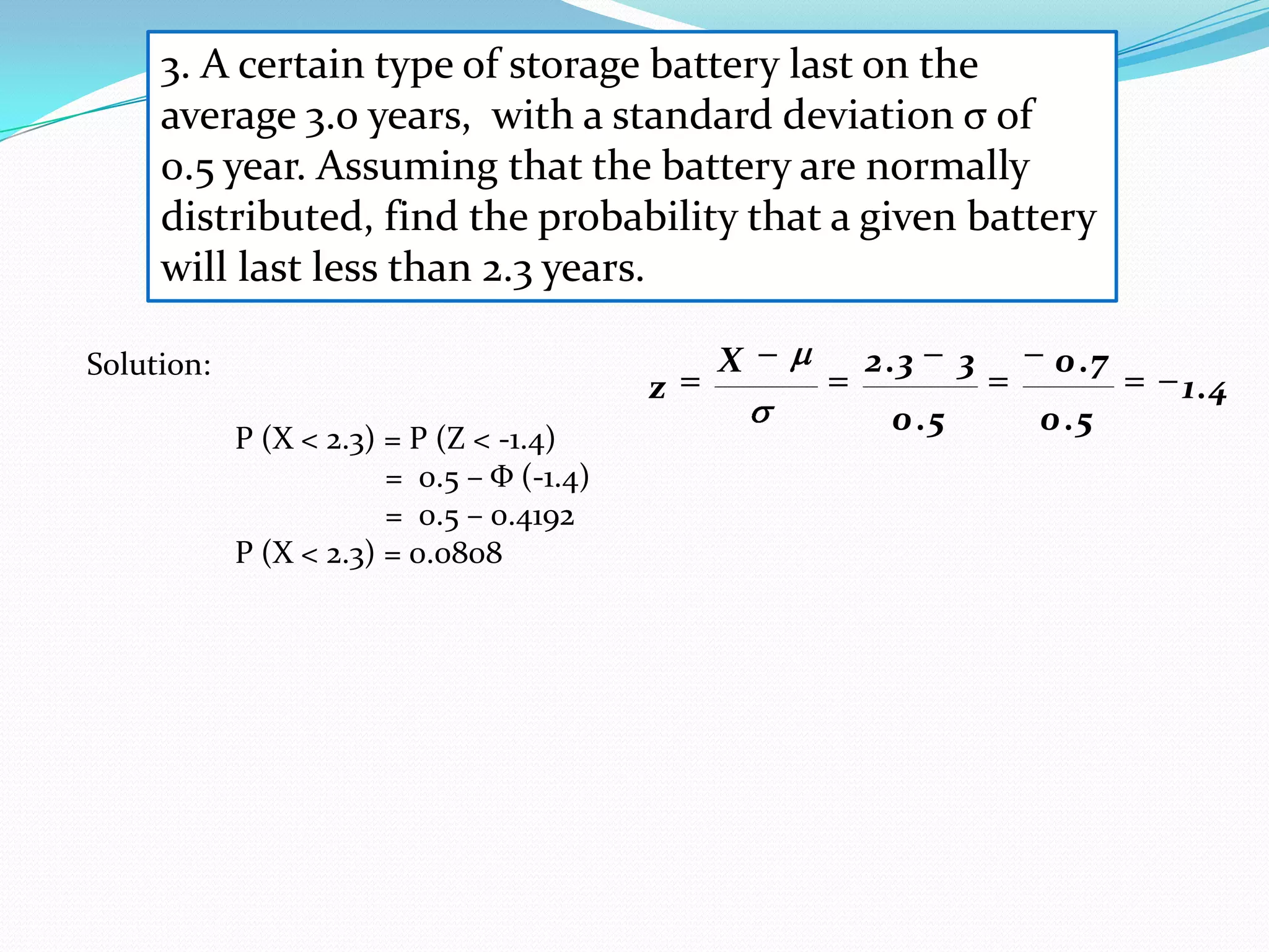
3. A certaintype of storage battery last on the
average 3.0 years, with a standard deviation σ of
0.5 year. Assuming that the battery are normally
distributed, find the probability that a given battery
will last less than 2.3 years.
Solution: X 2 .3 3 0 .7
z 1.4
0 .5 0 .5
P (X < 2.3) = P (Z < -1.4)
= 0.5 – Φ (-1.4)
= 0.5 – 0.4192
P (X < 2.3) = 0.0808